Characterizing Climate-Driven Shifts in Chilean Rainfall Regimes with a Hybrid Hidden Markov–Copula Framework

Chile's hydroclimate exhibits pronounced meridional gradients and strong interannual variability, posing persistent challenges for regime-aware, probabilistic rainfall prediction. We introduce a hierarchical framework that explicitly separates large-scale regime dynamics from local spatial dependence. The approach integrates: (i) a covariate-driven non-homogeneous Hidden Markov Model (nHMM) to identify synoptic precipitation regimes and their climate-sensitive transitions; (ii) Dynamic Time Warping (DTW) clustering to delineate precipitation-coherent climatic zones; and (iii) state-conditional Regular Vine copulas with Generalized Pareto (GPD) tails to model residual spatial dependence and extremes. The analysis employs the 0.05° daily CR2MET precipitation product over continental Chile (462 grid points, May–August (MJJA) 1980–2021) together with large-scale atmospheric covariates including zonal and meridional wind components, geopotential height, sea-level pressure, sea surface temperature, vertically integrated moisture flux and its divergence, and standard El Niño–Southern Oscillation (ENSO) indices: the Southern Oscillation Index (SOI), the Oceanic Niño Index (ONI), and the Global Mean Sea Surface Temperature (GMSST).

Five physically consistent rainfall regimes emerge, spanning from an anticyclonic dry state to a cyclonic wet state, confirmed by composites of mean sea-level pressure, 850 hPa winds, and 500 hPa geopotential height. The nHMM comprises p=29 284 estimated parameters fit to N_obs=2 386 692 daily observations ($N_{\mathrm{obs}}/p\approx \mathrm{82}$), confirming adequate model identifiability. Mixed-effects inference on annual transition proportions reveals a statistically significant decline in wet-state self-persistence of ≈0.34 % yr⁻¹ (95 % CI: [0.21, 0.47] % yr⁻¹; ≈14.5 % over 1980–2022), coincident with rising GMSST. Out-of-sample ensembles for MJJA 2022 (100 daily members conditioned on Viterbi-decoded states) are well calibrated across all seven DTW zones: central 90 % prediction intervals achieve near-nominal coverage (88 %–98 %), asymmetry degrees ≤ 0.07, and widths that increase monotonically southward with climatological variance. GPD shape parameters range from $\widehat{\mathit{\xi }}<\mathrm{0}$ in anticyclonic dry states (bounded tails) to $\widehat{\mathit{\xi }}>\mathrm{0}$ in episodic frontal states (heavy tails), confirming state-specific extreme behaviour. The vine-copula layer yields statistically significant improvements over a conditionally independent baseline (Diebold–Mariano test with heteroskedasticity- and autocorrelation-consistent standard errors, p<0.001) in the rainfall-active southern zones, where skill scores of the Continuous Ranked Probability Score reach 0.51 (Zone 5) and 0.35 (Zone 6) relative to a climatological benchmark, and the area under the receiver operating characteristic curve exceeds 0.87 for the 25 mm exceedance threshold. By disentangling regime timing and drivers from residual spatial co-variability and extremes, the proposed nHMM–DTW–vine–GPD framework yields meteorologically coherent states, spatially consistent probabilistic simulations, and quantitatively validated forecasts, offering a principled pathway for regime-conditioned, uncertainty-aware precipitation prediction to support hydroclimate risk management in Chile and other topographically complex regions.

1 Introduction

Understanding precipitation variability and its long-term modulation is a central challenge in hydroclimatology, particularly in regions of pronounced climatic heterogeneity such as Chile (Sarricolea et al., 2017). The country spans an extreme meridional gradient – from hyperarid deserts in the north (18–26° S) to temperate and subpolar climates in the south (44–54° S) – producing sharp transitions in precipitation regimes and associated hydrological processes. Rainfall variability operates across multiple temporal scales, including seasonal (Montecinos and Aceituno, 2003; Garreaud et al., 2009), interannual (Garreaud et al., 2017; Montecinos et al., 2011), and decadal to multidecadal fluctuations (Garreaud, 2009; Latoja et al., 2025). Among the large-scale climate drivers, El Niño–Southern Oscillation (ENSO) dominates interannual variability, modulating storm-track position, jet strength, and moisture transport toward subtropical South America (Trenberth, 2014; Robertson et al., 2004; Montecinos and Aceituno, 2003). These effects are typically represented through the Southern Oscillation Index (SOI), the Oceanic Niño Index (ONI), and the Global Mean Sea Surface Temperature (GMSST), which encapsulate large-scale forcing but often fail to explain the strong spatial gradients in rainfall induced by orography, mesoscale dynamics, and land–atmosphere coupling (Vrac and Friederichs, 2015; Bárdossy and Pegram, 2010).

The persistence of extreme drought conditions – particularly the decade-long “megadrought” affecting central Chile since 2010 (Garreaud et al., 2020; Bozkurt et al., 2021) – underscores the urgency of developing analytical frameworks that integrate both large-scale climate drivers and localized hydrological responses. Annual precipitation deficits between 15 % and 45 % relative to the pre-2010 baseline (Boisier et al., 2018), combined with regional warming and snowpack decline (Burger et al., 2018; Barría et al., 2019), have exacerbated water scarcity and altered runoff regimes. These changes highlight the limitations of traditional statistical models that assume linearity or stationarity (Charles et al., 2014; Wilks, 2011). Capturing hidden or emergent shifts in rainfall regimes therefore requires probabilistic frameworks capable of representing temporal evolution, regime persistence, and non-linear teleconnections.

In this context, we employ a Non-Homogeneous Hidden Markov Model (nHMM) to identify latent rainfall regimes and characterize their temporal dynamics. HMMs have been extensively used for atmospheric circulation regimes and daily rainfall sequences (Ailliot et al., 2009; Franzke and O'Kane, 2017); the non-homogeneous extension allows transition probabilities to depend on time-varying covariates such as ENSO indices or large-scale circulation fields (Hughes et al., 1999; Bellone et al., 2000; Robertson et al., 2004), enabling detection of evolving regime behavior under changing climatic conditions. Beyond identifying discrete rainfall states, we assess long-term persistence and transition probabilities using linear mixed models, quantifying statistically significant trends that reflect climate-induced shifts in regime stability.

A key limitation of conventional nHMM applications lies in their assumption of conditional spatial independence – that rainfall at different locations is independent once the hidden state is known. This simplification is rarely valid in complex terrain such as Chile, where strong orographic forcing and mesoscale circulations generate residual spatial dependence even after conditioning on large-scale atmospheric states. To address this, we develop a hybrid nHMM–Copula framework that combines the temporal structure and climatic interpretability of nHMMs with explicit spatial modelling via multivariate copulas. Chile is first partitioned into homogeneous precipitation zones using Dynamic Time Warping (DTW) clustering (Berndt and Clifford, 1994; Herrera et al., 2025). Within each zone, state-specific copula models reconstruct spatial dependence, thereby relaxing the restrictive independence assumption while preserving the probabilistic and physically interpretable structure of the HMM (Bárdossy and Pegram, 2010; Vrac and Friederichs, 2015).

Previous studies have independently applied HMMs and copula models to precipitation (Ailliot et al., 2009; Vrac and Friederichs, 2015), yet few have integrated spatial dependence within a covariate-driven nHMM framework. The novelty of this study lies in bridging these two perspectives through a hybrid regime-based, dependence-aware modelling system that explicitly links hidden rainfall regimes to large-scale atmospheric drivers while reconstructing state-conditioned spatial dependencies, providing an interpretable, transferable, and uncertainty-aware basis for rainfall regime analysis and probabilistic forecasting across Chile's diverse hydroclimatic zones.

The paper is organized as follows. Section 2 describes the data, the step-by-step model construction, and the validation approach. Section 3 presents the resulting rainfall regimes, their atmospheric interpretation, temporal trends, and spatially coherent probabilistic simulations. Section 4 discusses methodological advances, hydroclimatic implications, limitations, and potential extensions.

2 Data and Methods

This section guides the reader sequentially through the modelling pipeline. Section 2.1 describes the precipitation product and atmospheric covariates. Section 2.2 introduces the nHMM. Section 2.3 builds the hybrid spatial framework step by step: DTW zoning (Sect. 2.3.1), marginal specification (Sect. 2.3.2), copula construction (Sect. 2.3.3–2.3.4), simulation (Sect. 2.3.5), and uncertainty metrics (Sect. 2.3.6). Section 2.4 details the validation strategy. Section 2.5 summarizes model selection.

2.1 Data

Daily precipitation across Chile is monitored by official agencies (CR2, 2024), yet many ground stations exhibit discontinuities, missing data, or records shorter than 30 years, limiting their suitability for robust climate diagnostics. To ensure spatial completeness and temporal consistency, we employed the CR2MET dataset (Boisier, 2023; Boisier et al., 2018), a high-resolution (0.05°) gridded product developed specifically for continental Chile and validated against dense observational networks. CR2MET integrates station observations with ERA5 reanalysis (Hersbach et al., 2023) via statistical downscaling, capturing precipitation over complex orography more realistically than global products (Mayer et al., 2021; Cavalleri et al., 2024).

From CR2MET we extracted 462 grid points collocated with operational rain gauges with uninterrupted daily records during 1980–2021. Each grid point contributes $\mathrm{123}\times \mathrm{42}=\mathrm{5166}$ daily austral-winter (May–August; MJJA) observations; frontal systems during MJJA account for approximately 70 %–90 % of annual rainfall between 30 and 44° S (Pica-Téllez et al., 2020), dominating streamflow generation, groundwater recharge, and Andean snow accumulation (Valdés-Pineda et al., 2016). The year 2022 is reserved for out-of-sample evaluation. Seasonal totals are primarily modulated by the South Pacific Subtropical High and the Southern Hemisphere storm track (Hoskins and Hodges, 2005; Barrett and Hameed, 2017); orographic enhancement along the Andes intensifies rainfall from frontal systems (Garreaud et al., 2009; Arias et al., 2021), while persistent blocking can produce substantial deficits even during ENSO-neutral conditions (Latoja et al., 2025; Montecinos et al., 2011).

Large-scale atmospheric covariates for the nHMM transition model were extracted from ERA5 (Hersbach et al., 2023) at 0.25° × 0.25° over continental Chile and adjacent oceanic domains (15° N–60° S, 120–60° W). The covariate set comprises geopotential height at 500 hPa (Z500); mean sea-level pressure (MSLP); sea surface temperature (SST); near-surface and maximum temperature; zonal and meridional wind components at 850 hPa (u₈₅₀, v₈₅₀); vertically integrated moisture flux and its divergence (VIMF, VIMFD); and the ENSO indices SOI, ONI, and GMSST. The inclusion of VIMF and VIMFD is motivated by their direct link to landfalling moisture flux over Chile (Garreaud et al., 2009; Arias et al., 2021): u₈₅₀ and v₈₅₀ alone do not fully characterize atmospheric moisture delivery in the presence of orographic blocking and low-level jets. Principal Component Analysis was applied independently to each gridded field; leading components explaining more than 80 % of total variance were retained as predictors in the nHMM transition model.

2.2 Non-Homogeneous Hidden Markov Model

The nHMM (Khalil et al., 2010; Kirshner, 2005; Cioffi et al., 2020; Hughes et al., 1999; Robertson et al., 2004) identifies latent climate regimes and models their temporal evolution in daily rainfall sequences. Transitions between states follow the Markov property, and the nHMM extends the conventional HMM by allowing transition probabilities to vary in time through dependence on external covariates.

2.2.1 Model structure

Let $R_{t_i}^{{\mathit{r}}_j}$ denote daily precipitation at location ${\mathit{r}}_j=({\mathrm{long}}_j,{\mathrm{lat}}_j)$, $i=\mathrm{1},\mathrm{\dots },n$, $j=\mathrm{1},\mathrm{\dots },q$. In this study n=5166 (42 winters × 123 MJJA days, 1980–2021) and q=462 spatial locations; 2022 is reserved for out-of-sample evaluation. The q-dimensional precipitation vector on day t_i is ${\mathit{R}}_{t_i}=(R_{t_i}^{{\mathit{r}}_{\mathrm{1}}},\mathrm{\dots },R_{t_i}^{{\mathit{r}}_q})$, and the latent Markov chain $S_t\in \mathit{\{}\mathrm{1},\mathrm{\dots },K\mathit{\}}$ is defined by four assumptions.

Assumption 1 (Markovian dynamics): the hidden state sequence is first-order Markov, $P(S_{\mathrm{1}},\mathrm{\dots },S_n)=p\left(S_{\mathrm{1}}\right){\prod }_{t=\mathrm{2}}^{n}p(S_t\mid S_{t-\mathrm{1}})$.

Assumption 2 (Conditional rainfall dependence): $p({\mathit{R}}_{\mathrm{1}:n},S_{\mathrm{1}:n})=p\left(S_{\mathrm{1}}\right){\prod }_{t=\mathrm{2}}^{n}p(S_t\mid S_{t-\mathrm{1}}){\prod }_{t=\mathrm{1}}^{n}p({\mathit{R}}_t\mid S_t)$.

Assumption 3 (Conditional spatial independence): conditional on S_t, precipitation across stations is assumed independent, $p({\mathit{R}}_t\mid S_t)={\prod }_{m=\mathrm{1}}^{q}p(R_t^m\mid S_t)$. This assumption is relaxed in Sect. 2.3 via vine copulas. Each marginal term follows a zero-inflated Gamma mixture,

$$p(R_t^m\mid S_t=i)=\left\{\begin{array}{ll}{p}_{im\mathrm{0}},& R_t^m=\mathrm{0},\\ {\sum }_{c=\mathrm{1}}^{C-\mathrm{1}}\frac{p_{im\mathrm{1}}{\mathit{\varphi }}_{imc}^{{\mathit{\omega }}_{imc}}(R_t^m{)}^{{\mathit{\omega }}_{imc}-\mathrm{1}}{e}^{-{\mathit{\varphi }}_{imc}{R}_t^m}}{\mathrm{\Gamma }\left({\mathit{\omega }}_{imc}\right)},& R_t^m>\mathrm{0},\end{array}\right.$$

where p_im0 is the dry-day probability, $p_{im\mathrm{1}}=\mathrm{1}-p_{im\mathrm{0}}$, and (ω_imc,ϕ_imc) are shape and rate parameters of the cth Gamma component.

Assumption 4 (Non-homogeneity): transition probabilities depend on the atmospheric covariate vector ${\mathit{X}}_t=(X_t^{\mathrm{1}},\mathrm{\dots },X_t^h)$ via multinomial logistic regression,

$$p(S_t=i\mid S_{t-\mathrm{1}}=j,{\mathit{X}}_t=\mathit{x})={\displaystyle \frac{\exp ({\mathit{\alpha }}_{j,i}+{\mathit{\beta }}_i^T\mathit{x})}{{\sum }_{k=\mathrm{1}}^K\exp ({\mathit{\alpha }}_{j,k}+{\mathit{\beta }}_k^T\mathit{x})}},$$

where α_j,i is the baseline log-odds of transition j→i and β_i quantifies covariate influence.

2.2.2 Estimation

Parameters are estimated via the Baum–Welch (EM) algorithm (McLachlan and Krishnan, 2008), following Kirshner (2005) as adapted by Robertson et al. (2006). Model selection over $K\in \mathit{\{}\mathrm{2},\mathrm{\dots },\mathrm{6}\mathit{\}}$ and $C\in \mathit{\{}\mathrm{2},\mathrm{\dots },\mathrm{8}\mathit{\}}$ uses AIC and BIC (Sect. 2.5).

2.3 Hybrid nHMM–Copula Framework with DTW-Based Zoning

The nHMM provides a coherent temporal-regime layer, but Assumption 3 is often too restrictive in regions with strong orographic gradients and mesoscale circulations such as Chile (Becker and Schmitz, 2003; Garreaud, 2009; Sarricolea and Meseguer-Ruiz, 2017). The hybrid framework addresses this through four sequential steps whose conceptual justification is elaborated in Sect. 2.4.4. Full mathematical details and extended diagnostics are in Supplement S1–S4.

2.3.1 Step 1 – Zoning via DTW

A direct q=462-variate copula is computationally prohibitive. We partition the station network into k^∗ zones via hierarchical clustering on pairwise Dynamic Time Warping (DTW) dissimilarities computed from standardized MJJA daily series (Berndt and Clifford, 1994; Giorgino, 2009; Montero and Vilar, 2015):

$$\mathrm{DTW}(i,j)=\underset{\mathit{\pi }\in {\mathrm{\Pi }}_{ij}}{min}\sum _{(\mathit{\tau },\mathit{\kappa })\in \mathit{\pi }}\Vert y_i\left(\mathit{\tau }\right)-y_j\left(\mathit{\kappa }\right)\Vert ,$$

where Π_ij is the set of monotone warping paths. Ward's linkage (Ward, 1963) on the resulting distance matrix yields compact, interpretable clusters.

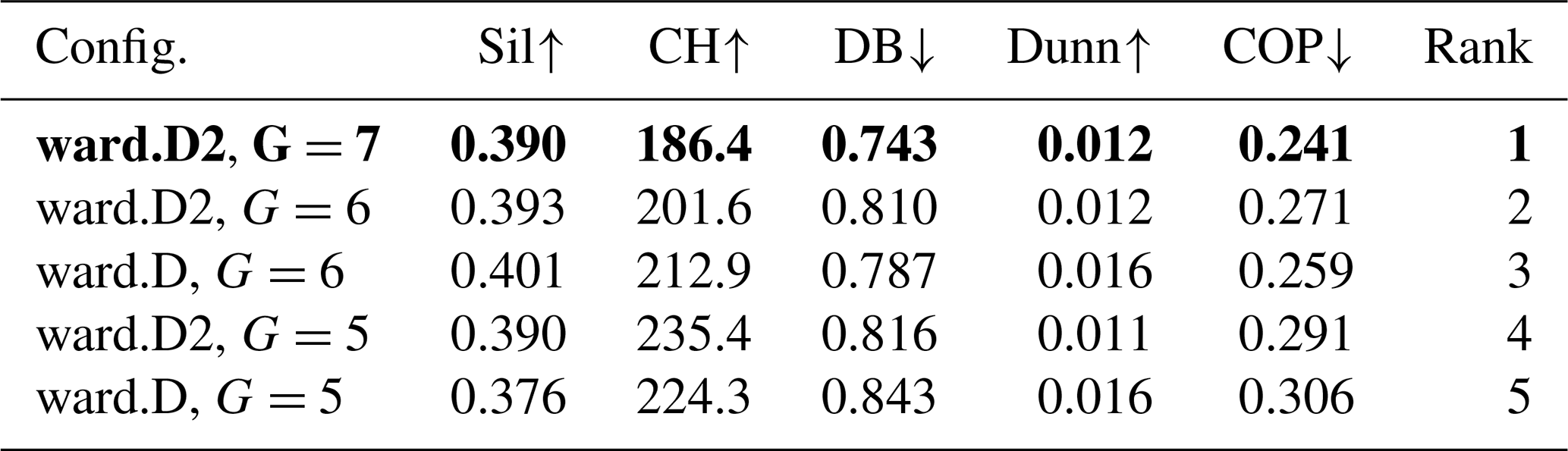
The optimal number of zones is $k^{\ast }=\mathrm{7}$, selected via a consensus of five internal cluster validity indices (CVI): Silhouette, Calinski–Harabasz, Davies–Bouldin, Dunn, and COP (Table 1; full table in Supplement S2). The G=7 solution achieves the best consensus rank across all five CVIs, aligns with established climatic subregions of continental Chile (Sarricolea et al., 2017; Garreaud et al., 2009), and yields zones with $d_z\in [\mathrm{50},\mathrm{90}]$ stations and at least 200 training days per state, providing sufficient data for robust copula estimation.

Table 1 Top-ranked DTW zoning candidates (consensus CVI rank). Sil: Silhouette; CH: Calinski–Harabasz ($\times {\mathrm{10}}^{-\mathrm{1}}$); DB: Davies–Bouldin; COP: COP index. ↑: larger is better; ↓: smaller is better. Bold: selected configuration.

2.3.2 Step 2 – State-conditional marginal specification

For station m in zone z and regime s, the state-conditioned CDF $F_{m,s}\left(x\right)=\mathbb{P}(R_t^m\le x\mid S_t=s)$ is estimated from the Viterbi-decoded training subset using a three-part hybrid marginal: (1) a point mass at zero with probability $p_{m,s}^{\left(\mathrm{0}\right)}=\mathbb{P}(R_t^m=\mathrm{0}\mid S_t=s)$; (2) a (C−1)-component Gamma mixture for positive amounts; and (3) a Generalized Pareto Distribution (GPD) for the upper tail above threshold u_m,s (0.90 empirical quantile of positive precipitation):

$$\mathbb{P}(Y\le y)=\mathrm{1}-{\left(\mathrm{1}+{\displaystyle \frac{{\mathit{\xi }}_{m,s}y}{{\mathit{\sigma }}_{m,s}}}\right)}_{+}^{-\mathrm{1}/{\mathit{\xi }}_{m,s}},y=x-u_{m,s}\ge \mathrm{0}.$$

Continuity of F_m,s at u_m,s is enforced by probability-splicing (Hughes et al., 1999; Khalil et al., 2010; Bárdossy and Pegram, 2010; Vrac and Naveau, 2007).

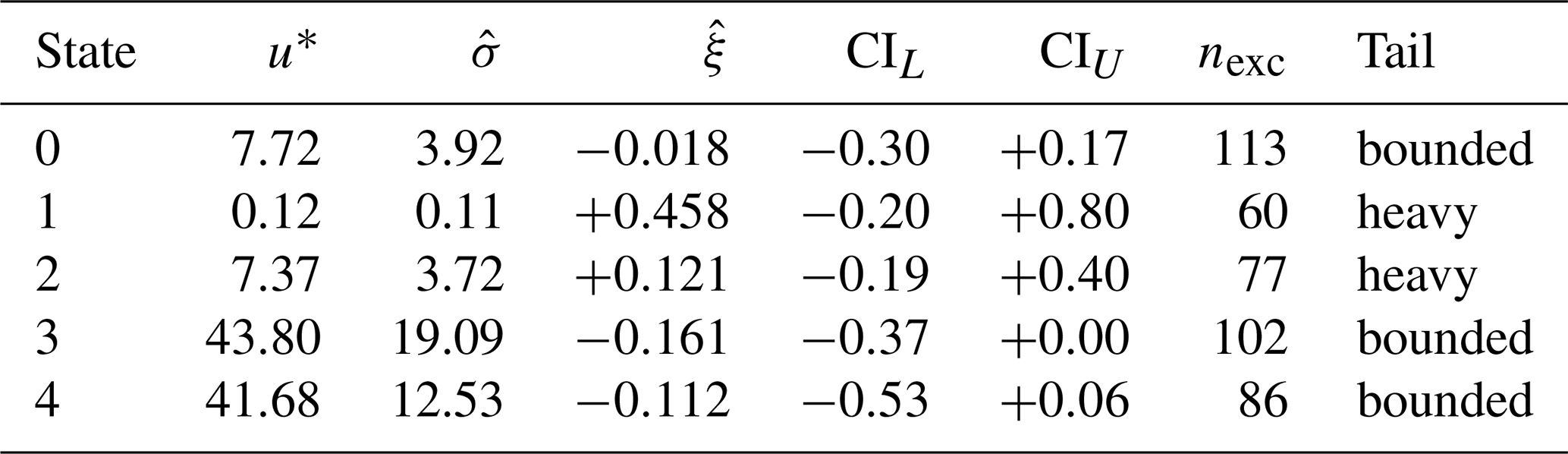
Table 2 summarizes GPD estimates for the Zone 5 medoid (southern Chile, storm-dominated) across all five states. GPD shape parameters exhibit a physically consistent pattern: states 0, 3, and 4 (anticyclonic to transitional) show $\widehat{\mathit{\xi }}\le \mathrm{0}$ (bounded or near-exponential tails), while states 1 and 2 (episodic frontal intrusions) yield $\widehat{\mathit{\xi }}>\mathrm{0}$ (heavy, unbounded tails). This contrast reflects the distinct precipitation generation mechanisms: light, intermittent precipitation associated with cold-air incursions under blocking conditions (bounded tails) versus intense, organized rainfall from deep frontal systems (heavy tails). Bootstrap 95 % confidence intervals (B=500 parametric resamples of the medoid's own exceedances) confirm that this sign contrast is statistically robust across the range. Threshold sensitivity at $u_{m,s}\in [\mathrm{0.85},\mathrm{0.95}]$ was verified via mean-excess diagnostics (Supplement S3), confirming adequate GPD stability at the adopted 0.90 level.

Table 2 GPD parameter estimates at the Zone 5 medoid by nHMM state (southern Chile, storm-dominated). u^∗: 0.90-quantile threshold (mm); $\widehat{\mathit{\sigma }}$: scale; $\widehat{\mathit{\xi }}$: shape; 95 % bootstrap CI from B=500 parametric resamples of medoid exceedances; n_exc: number of exceedances above u^∗.

2.3.3 Step 3 – Transformation to copula space

State-conditional probability integral transform (PIT) pseudo-observations for zone z and regime s are defined as $U_t^{\left(m\right)}=F_{m,s}\left(R_t^m\right)$, $m=\mathrm{1},\mathrm{\dots },d_z$. By Sklar's theorem (Nelsen, 2006; Genest and MacKay, 1986), the conditional joint law factorizes as

$$F_{z,s}\left(\mathit{r}\right)=C_{z,s}\left(F_{\mathrm{1},s}\right(r_{\mathrm{1}}),\mathrm{\dots },F_{d_z,s}(r_{d_z}\left)\right),$$

so marginal behaviour is inherited from Step 2 and residual spatial dependence is encoded entirely by the copula C_z,s.

2.3.4 Step 4 – Regular vine construction and model selection

For d_z up to ∼ 90 we represent C_z,s by a Regular Vine (R-vine) (Aas et al., 2009), decomposing the d_z-variate density into bivariate pair-copulas:

$$c_{z,s}(u_{\mathrm{1}},\mathrm{\dots },u_{d_z})=\prod _{m=\mathrm{1}}^{d_z-\mathrm{1}}\prod _{e\in E_m}{c}_e(u_{i|D},u_{j|D};{\mathit{\theta }}_e).$$

We adopt the simplifying assumption (pair-copula parameters independent of conditioning variable values); diagnostics in Sect. 2.4.2 confirm its empirical adequacy. The candidate family set is $\mathcal{F}=\mathit{\{}\mathrm{Gaussian},\mathrm{Student}\text{-}t,\mathrm{Clayton},\mathrm{Gumbel},\mathrm{Frank}\mathit{\}}$, covering elliptical and Archimedean families with different tail properties. Structure selection and family assignment use AIC edge-wise via RVineStructureSelect (Schepsmeier et al., 2015); parameters are estimated by maximum likelihood with multiple random initialisations. Vines are truncated at Tree 2, which captures the dominant spatial links (typically between nearby stations) while limiting over-fitting in higher-order trees where conditional dependence attenuates.

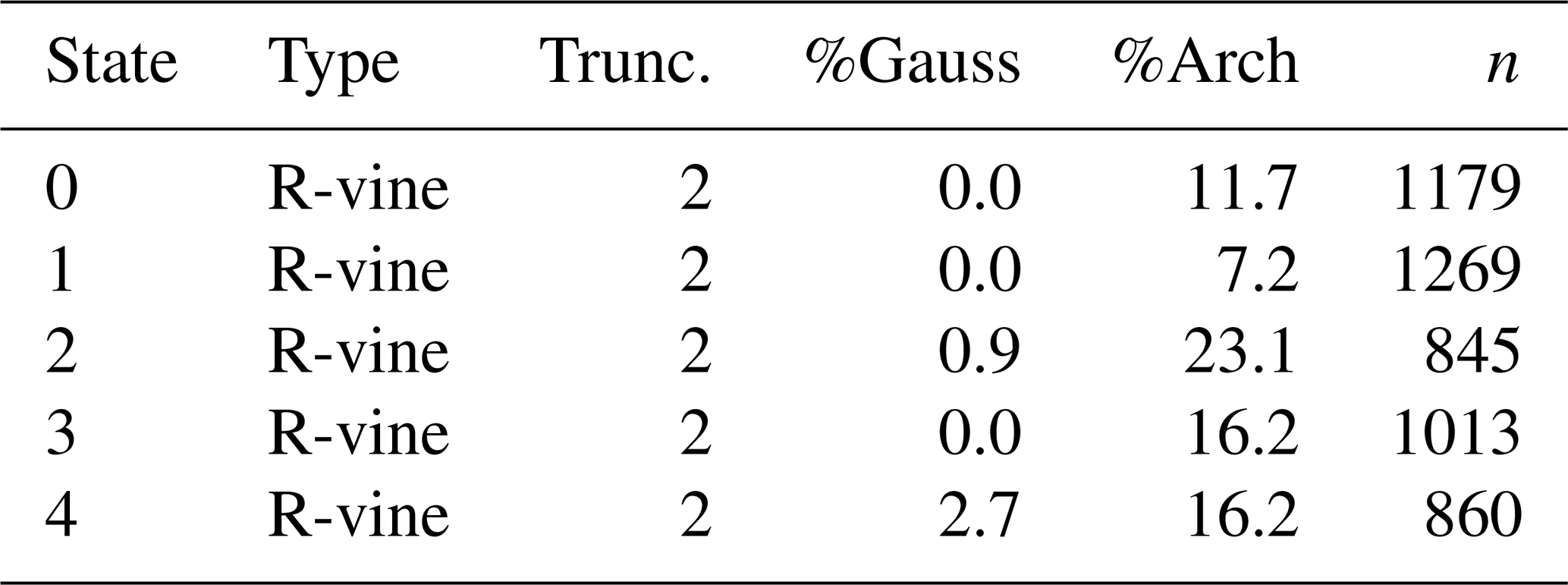
Table 3 shows the selected structures for Zone 2 (semi-arid north) across all states. All are R-vines truncated at Tree 2, with Archimedean families predominating (7 %–23 % of edges) and Gaussian pairs rare (0 %–3 %), reflecting the non-Gaussian, asymmetric spatial dependence structure of daily precipitation in semi-arid terrain. As expected, the proportion of Gaussian pairs increases southward (reaching ∼ 22 % in wet states of Zone 5; Supplement S4), consistent with more elliptically distributed spatial fields under persistent frontal forcing.

Table 3 Selected vine structures for Zone 2, all five states. %Arch: percentage of Archimedean pair-copula families selected by AIC; n: training days.

2.3.5 State-aware simulation and back-transformation

Given Viterbi-decoded regime ${\widehat{S}}_t$ for day t and zone z: (1) draw ${\mathit{U}}_t^z\sim C_{z,{\widehat{S}}_t}$ via RVineSim; (2) map back to precipitation using the stitched marginal inverse, directing draws above the tail threshold through the GPD quantile function (Trenberth, 2014; Franzke and O'Kane, 2017). The full system comprises $\mathrm{7}\times \mathrm{5}=\mathrm{35}$ copula models, parallelized across (z,s) using VineCopula (Schepsmeier et al., 2015) and TSclust (Montero and Vilar, 2015).

2.3.6 Uncertainty quantification metrics

From M ensemble members per day, define the central 90 % prediction interval $[{\widehat{L}}_t,{\widehat{U}}_t]$ (5th–95th percentiles). Let $X_t^{\mathrm{obs}}$ be the observation. We report the Average Width (AW), the Percentage of Coverage (POC), and the Average Asymmetry Degree (AAD):

$$\begin{array}{c}{\displaystyle }\mathrm{AW}=\frac{\mathrm{1}}{T}\sum _t({\widehat{U}}_t-{\widehat{L}}_t),\\ {\displaystyle }\mathrm{POC}=\frac{\mathrm{1}}{T}\sum _t\mathbf{1}\mathit{\{}{X}_t^{\mathrm{obs}}\in [{\widehat{L}}_t,{\widehat{U}}_t\left]\mathit{\right\}},\\ {\displaystyle }\mathrm{AAD}=\frac{\mathrm{1}}{T}\sum _t{\mathrm{AAD}}_t,\end{array}$$

where AAD_t measures the normalized distance of the observation from the nearest interval bound when outside (and is zero when inside). These indicators are not substitutes for proper scoring rules but enhance communication of sharpness, calibration, and directional bias across zones.

2.4 Model validation strategy

We assess model adequacy at two complementary levels: the temporal regime structure encoded by the nHMM, and the residual state-conditioned spatial dependence within DTW zones. Probabilistic skill is verified out-of-sample. Each diagnostic component is described below together with its decision criterion, clarifying how each test leads to a specific modelling choice rather than serving merely as a catalogue of tests applied.

2.4.1 nHMM fit and calibration

The nHMM yields the one-step predictive distribution $\mathcal{L}(R_t^m\mid {\mathcal{F}}_{t-\mathrm{1}})={\sum }_{s=\mathrm{1}}^K\mathrm{Pr}(S_t=s\mid {\mathcal{F}}_{t-\mathrm{1}})\mathcal{L}(R_t^m\mid S_t=s)$, where ${\mathcal{F}}_{t-\mathrm{1}}=\mathit{\sigma }\mathit{\{}{\mathit{R}}_{\mathrm{1}:t-\mathrm{1}},{\mathit{X}}_{\mathrm{1}:t}\mathit{\}}$. PIT residuals $U_{t,m}=F_{t,m}\left(R_t^m\right)$ should be i.i.d. Unif(0,1) under correct specification (Dawid, 1984; Gneiting and Raftery, 2007). We examine PIT histograms and apply Kolmogorov–Smirnov (KS) and Cramér–von Mises (CvM) uniformity tests, together with Ljung–Box tests for residual autocorrelation (Supplement S1). Retention criterion: a configuration is retained if PIT histograms are visually flat, KS/CvM tests do not reject uniformity at the 5 % level for >80 % of stations, and no significant Ljung–Box autocorrelation is detected. Regime count K is selected by BIC (Sect. 2.5), with PIT-based adequacy as a secondary check. Wet/dry occurrence is validated via Brier scores and reliability diagrams; tail diagnostics include mean-excess plots and GPD shape bootstrap CIs (Supplement S3). State-aware PITs using smoothed probabilities ${\sum }_s\mathrm{Pr}(S_t=s\mid {\mathit{R}}_{\mathrm{1}:n},{\mathit{X}}_{\mathrm{1}:n})F_{m,s}(\cdot )$ isolate emission misspecification from transition errors (Zucchini et al., 2016).

2.4.2 Vine-copula fit: residual spatial dependence

Within zone z and regime s, the Rosenblatt transform ℛ_z,s maps ${\mathit{U}}_t^z$ to components ${\mathit{V}}_t^z$ that should be i.i.d. Unif(0,1) under correct specification (Rosenblatt, 1952). Diagnostics include marginal KS/CvM tests on ${\mathit{V}}_t^z$; energy-distance tests against $\mathrm{Unif}\left(\right[\mathrm{0},\mathrm{1}{]}^{d_z})$ (Székely and Rizzo, 2013); and parametric-bootstrap GoF for edge copulas (Genest and Rémillard, 2008; Genest et al., 2009). Upper tail-coincidence rates ${\widehat{\mathit{\lambda }}}_U\left(\mathrm{0.95}\right)$ and variogram functionals γ_α(u) are reported in Supplement S4. We note that KS and CvM tests on individual Rosenblatt components are extremely sensitive at the training sample sizes employed here (n=845–1269 d per state): they will reliably detect even minor residual dependence that has negligible practical consequence for forecast calibration. Accordingly, the operative criterion for vine adequacy is not strict p-value thresholds on every component but rather: (i) PIT histograms visually consistent with uniformity for states and zones used in the verification; (ii) variogram scores lower for the vine model than for the independence baseline; and (iii) Diebold–Mariano tests confirming predictive skill gains in out-of-sample verification. Competing vine structures (C-, D-, R-vines), truncation levels, and family sets are compared by AIC/BIC; Vuong's test resolves close comparisons (Vuong, 1989).

2.4.3 Out-of-sample probabilistic verification

We use strictly proper scoring rules (Gneiting and Raftery, 2007). The Continuous Ranked Probability Score (CRPS) for a predictive CDF F and realization y is

$$\mathrm{CRPS}(F,y)=\underset{-\mathrm{\infty }}{\overset{\mathrm{\infty }}{\int }}\left(F\right(x)-\mathbf{1}\mathit{\{}x\ge y\mathit{\}}{)}^{\mathrm{2}}\mathrm{d}x,$$

estimated from ensemble $\mathit{\{}{Y}^{\left(m\right)}{\mathit{\}}}_{m=\mathrm{1}}^M$ via the unbiased estimator of Gneiting and Raftery (2007). CRPS skill scores (CRPSS) use the MJJA climatological distribution (1980–2021) as the reference. At the multivariate level, energy scores (ES) and variogram scores (VS) (Scheuerer and Hamill, 2015) are computed; VS is particularly diagnostic of dependence misspecification. Differences versus the conditionally independent baseline are tested with Diebold–Mariano statistics using Newey–West heteroskedasticity- and autocorrelation-consistent (HAC) standard errors (Diebold and Mariano, 1995; Bergmeir and Benítez, 2012). Decision criterion: the vine layer is deemed to improve over the independence baseline if the Diebold–Mariano test rejects equality at the 10 % level (HAC-adjusted) for station-wise CRPS or zone-wise VS in the majority of zones.

2.4.4 Conceptual justification of the hierarchical design

The apparent tension between assuming conditional spatial independence in the nHMM (Assumption 3) and subsequently introducing spatial dependence via copulas is resolved by scale separation. Regime transitions are driven by synoptic–planetary variability (ENSO, storm track, South Pacific High), whereas subdaily–mesoscale organization shapes spatial correlation given a regime. Estimating regimes without a high-dimensional spatial likelihood avoids confounding temporal state dynamics with local dependence and stabilizes identification of K, transition coefficients, and emission parameters. The modular likelihood is computationally tractable ($N_{\mathrm{obs}}/p\approx \mathrm{82}$ at the nHMM stage) and attains near-full-model performance without embedding a d_z-variate copula inside EM. Any potential mismatch introduced by the modular approach is explicitly probed by the three-layer diagnostic strategy above. Empirically, the copula-adjusted simulations reproduce observed spatial coherence and extreme-rainfall behaviour in the rainfall-active zones (Sect. 3), providing the key evidence that this principled approximation is adequate for the intended purpose.

2.5 Model selection: grid of nHMM configurations

We fitted a grid of 30 nHMMs varying $K\in \mathit{\{}\mathrm{2},\mathrm{\dots },\mathrm{6}\mathit{\}}$ and the number of Gamma mixture components $C\in \mathit{\{}\mathrm{2},\mathrm{\dots },\mathrm{8}\mathit{\}}$ (Supplement S9), denoting each as KhsCdg. Model selection uses $\mathrm{BIC}=p\log N_{\mathrm{obs}}-\mathrm{2}\mathrm{\ell }\left(\widehat{\mathit{\theta }}\right)$ where $N_{\mathrm{obs}}=\mathrm{5166}\times \mathrm{462}=\mathrm{2}\mathrm{386}\mathrm{692}$. Table 4 reports key statistics for the three candidate models.

Table 4 Model selection: representative configurations per K (by BIC). ℓ: maximized log-likelihood; p: free parameters; $N/p$: observations-per-parameter ratio. Bold: adopted configuration. The BIC minimum within K=5 is 5hs3dg (BIC =10 437 601); 5hs5dg is preferred on secondary criteria (PIT flatness, regime separation, GPD tail adequacy) at a BIC cost of <0.5 %. Full 30-configuration grid in Supplement S9.

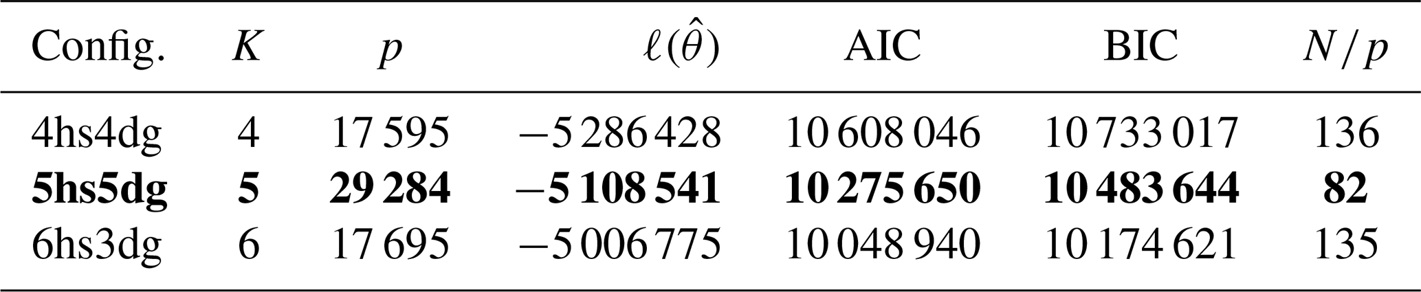
The BIC surface shows a clear elbow at K=5: moving from K=4 to K=5 yields a large likelihood gain that compensates the penalty, while K=6 increases p sharply with negligible improvement and produces weakly separated regimes confirmed by regime-overlap diagnostics (Supplement S9). Within K=5, the ratio $N/p\approx \mathrm{82}$ confirms adequate identifiability: there are roughly 82 observations per estimated parameter. We adopt K=5, C=5 for all subsequent analyses.

3 Results

3.1 Overview of model configuration

All results use nHMM 5hs5dg (K=5, C=5; p=29 284; $N/p\approx \mathrm{82}$) with residual spatial dependence modelled within G=7 DTW zones (Table 1), each with $d_z\in [\mathrm{50},\mathrm{90}]$ stations. For each zone and state, a state-conditional R-vine copula (Table 3) is fit by maximum likelihood estimation (MLE) and used for ensemble simulation. Forecast verification employs central 90 % prediction interval diagnostics (POC, AW, AAD) and strictly proper scoring rules (CRPS, ES, VS) under blocked cross-validation and out-of-sample tests (Tables 6–7; Supplement S5–S9).

3.2 Climatic organization of precipitation by hidden Markov states

Figure 1 synthesizes austral-winter (MJJA) precipitation conditioned on the five nHMM regimes. For each column, the main map shows the conditional mean daily precipitation (mm d⁻¹) across the 462 locations for days assigned to that state by the Viterbi path; the inset displays anomalies relative to the MJJA climatology (1980–2021). Climatologically, conditional means peak over southern Chile (40–55° S), consistent with vigorous mid-latitude cyclone activity and Andean orographic enhancement. Northern Chile (north of 30° S) remains dry in all regimes. The anomaly insets reveal a coherent dry-to-wet progression: regimes “0” and “1” exhibit widespread negative anomalies (suppressed frontal activity); regime “2” presents near-neutral, spatially patchy anomalies; and regimes “3” and “4” display robust positive anomalies from ≈ 35 to ≈ 45° S, enhanced by windward ascent.

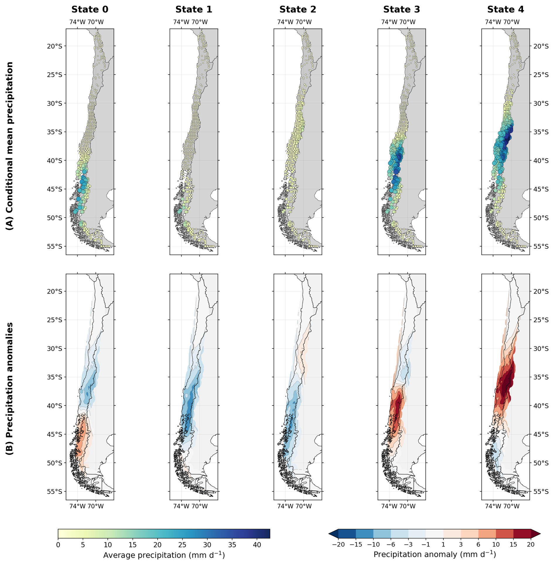
Figure 1 Mean precipitation and anomalies by nHMM state (MJJA, 1980–2021). (A) Conditional mean daily precipitation (mm d⁻¹) across the 462 locations for each of the five latent states; marker size and colour are proportional to the conditional mean. (B) Precipitation anomalies (mm d⁻¹) relative to the MJJA climatology, shown as full-size interpolated maps for readability. States “0”/“1”: dry regimes; “2”: transitional; “3”/“4”: wet regimes, strongest over ≈ 35–45° S.

Figure 2 shows circulation composites for each state. Dry states (e.g., “1”): a ridge–high couplet with positive Z500 over the southeast Pacific and positive MSLP over central Chile displaces the storm track poleward and strengthens subsidence over 30–40° S; weakened westerlies and enhanced coastal southerlies inhibit onshore moisture flux and orographic triggering. Wet states (e.g., “4”): a deep negative Z500 trough extending from the Amundsen–Bellingshausen sector, paired with a negative MSLP minimum south of ≈40° S, intensifies a zonal low-level jet impinging on central–southern Chile; cyclonic curvature favours frontal genesis and baroclinic development. Transitional states (“0”, “2”, “3”) show intermediate synoptic structures consistent with episodic storm incursions. The columnwise correspondence between the MSLP and Z500 composites evidences robust vertical coupling, while the 850 hPa streamlines underscore the state-dependent Pacific moisture corridor intersecting the Andes.

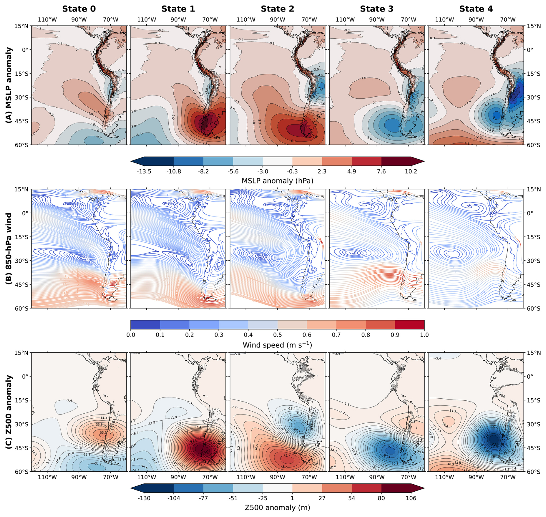
Figure 2 Circulation composites by nHMM state (MJJA, 1980–2021). (A) Mean sea-level pressure (MSLP) anomalies (hPa) relative to the MJJA climatology; (B) 850 hPa wind streamlines, coloured by normalized wind speed; (C) 500 hPa geopotential height (Z500) anomalies (m). Contour labels indicate anomaly magnitudes. Dry regimes (e.g., State 1): ridge–high couplet with weakened westerlies. Wet regimes (e.g., State 4): trough–low couplet with an intensified westerly jet impinging on central–southern Chile.

3.3 Persistence and inter-regime transitions

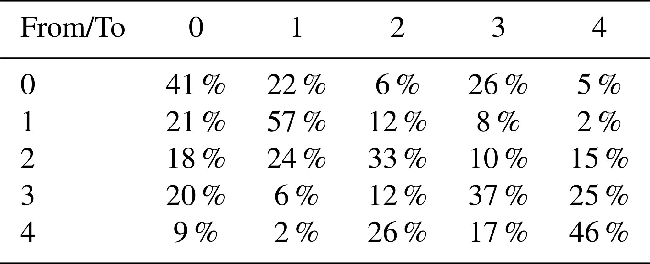
Table 5 reports the average empirical transition matrix for MJJA 1980–2022. The matrix is diagonally dominant, evidencing persistence: the dry regime S₁ has the largest self-transition probability (${\widehat{p}}_{\mathrm{11}}=\mathrm{0.57}$), followed by the wet regime S₄ (${\widehat{p}}_{\mathrm{44}}=\mathrm{0.46}$); S₀, S₂, S₃ are moderately persistent (0.33–0.41), acting as transitional configurations. Direct dry–wet jumps are rare (${\widehat{p}}_{\mathrm{14}}=\mathrm{0.02}$, ${\widehat{p}}_{\mathrm{41}}=\mathrm{0.02}$), dynamically consistent with the gradual synoptic reconfiguration required to transition between anticyclonic and deep cyclonic states (Franzke and O'Kane, 2017). Transitions among S₀–S₁–S₂ are relatively frequent, while S₃↔S₄ is favoured over links between wet and dry clusters, supporting S₃ as a preconditioning stage toward wetness.

Table 5 Average transition probabilities (MJJA, 1980–2022). Each entry is ${\widehat{p}}_{ij}$: the empirical probability of transition i→j given current state i. Bootstrap 95 % CIs (B=500 block bootstraps of annual MJJA seasons) showed widths ≤3 % for diagonal entries and ≤2 % for off-diagonal entries (not shown for conciseness).

Analysis of annual transition proportions $\mathit{\{}{p}_{ij}^{\left(y\right)}{\mathit{\}}}_{y=\mathrm{1980}}^{\mathrm{2022}}$ via binomial Generalized Linear Mixed Models (GLMMs; beta-binomial under overdispersion), with Benjamini–Hochberg False Discovery Rate (FDR) correction (Benjamini and Hochberg, 1995) over all K²=25 transition pairs, reveals a statistically significant decline in S₄→S₄ self-persistence at ≈0.34 % yr⁻¹ (95 % CI: [0.21, 0.47] % yr⁻¹; p<0.01), indicating shorter wet-regime residence over the study period (Figure 3). The S₁→S₁ self-persistence is trendless (p=0.43). Bridging transitions show compensating behaviour, with modest increases in 0↔3 alongside reduced 3→4 probability, suggesting more frequent cycling through transitional states rather than persistent wet occupancy. Approximately 73 % of the variance in $\mathit{\left\{}{p}_{ij}^{\left(y\right)}\mathit{\right\}}$ arises from systematic differences among transition pairs.

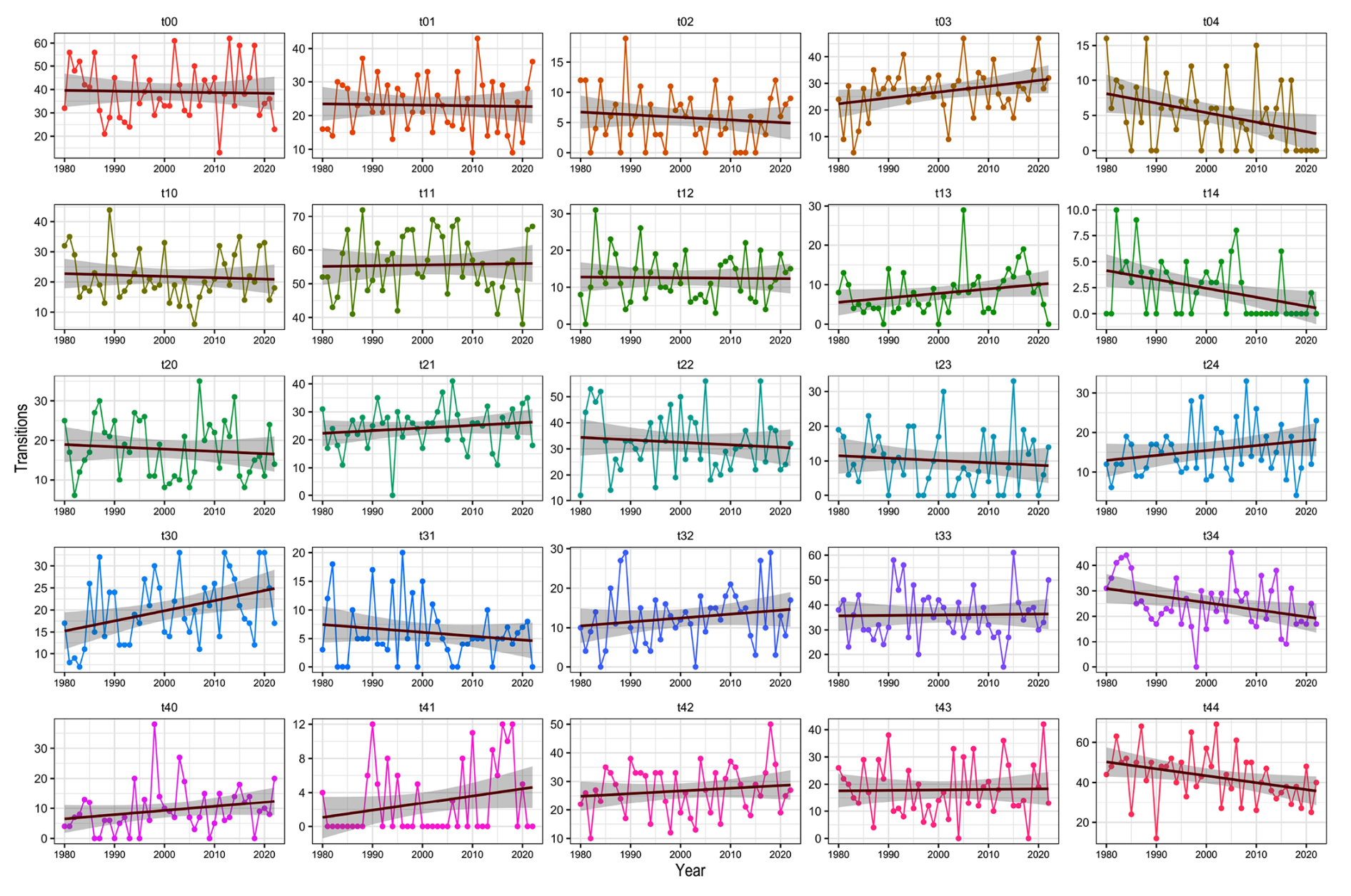
Figure 3 Annual transition proportions and Generalized Linear Mixed Model (GLMM) trends (MJJA, 1980–2022). Points: annual proportions $p_{ij}^{\left(y\right)}$. Solid lines: logit-linear GLMM trends (minimum 25 nonzero years, ${\sum }_y{C}_{ij}^{\left(y\right)}\ge \mathrm{100}$). Shaded bands: 95 % CIs. Red dashed: significant trend after BH-FDR correction (p<0.05).

3.4 Linkages between regimes and large-scale climate indices

Seasonal state occupancy $f_k\left(y\right)={\mathrm{123}}^{-\mathrm{1}}{\sum }_{t\in T_y}\mathrm{1}\mathit{\{}{S}_t=k\mathit{\}}$ is correlated with SOI, Niño 3.4, ONI, and GMSST (Fig. 4). Dry-state occupancy f₁ correlates positively with SOI and negatively with Niño/ONI; wet-state f₄ shows the opposite, consistent with canonical ENSO forcing (Montecinos and Aceituno, 2003; Garreaud et al., 2017). Transitional states ($k\in \mathit{\{}\mathrm{0},\mathrm{2},\mathrm{3}\mathit{\}}$) show weaker, sign-varying associations. GMSST relates negatively to f₄, consistent with increased subtropical stability and a poleward baroclinicity shift under global warming (Garreaud et al., 2020). The moderate magnitudes of $\left|{\mathit{\rho }}_{k,I}\right|$ reflect the well-established feature that ENSO modulates but does not deterministically control synoptic regimes; the copula component is motivated precisely by these nonlinear, tail-enhanced associations. Spearman and Kendall rank correlations yield qualitatively identical patterns; signs remain invariant under FDR control (Benjamini and Hochberg, 1995; Politis and Romano, 1994) and block-bootstrap uncertainty bounds (Supplement S7).

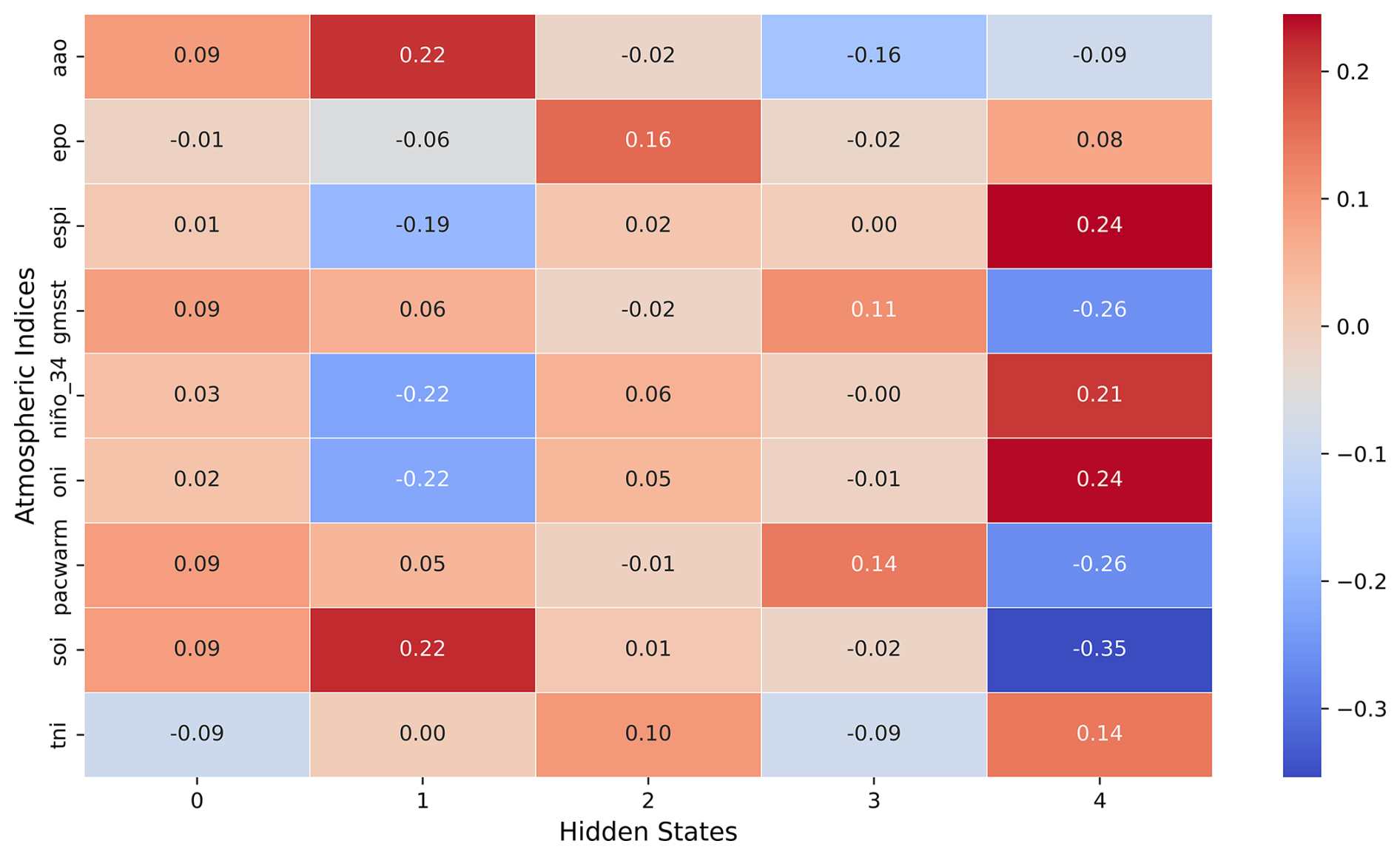
Figure 4 Pearson correlations between seasonal state frequencies and atmospheric indices (MJJA, 1980–2022). Asterisks: significant at the 5 % level after effective-sample-size correction (Pyper and Peterman, 1998). Signs agree with ENSO modulation; moderate magnitudes are consistent with teleconnections that modulate – not deterministically control – synoptic regimes.

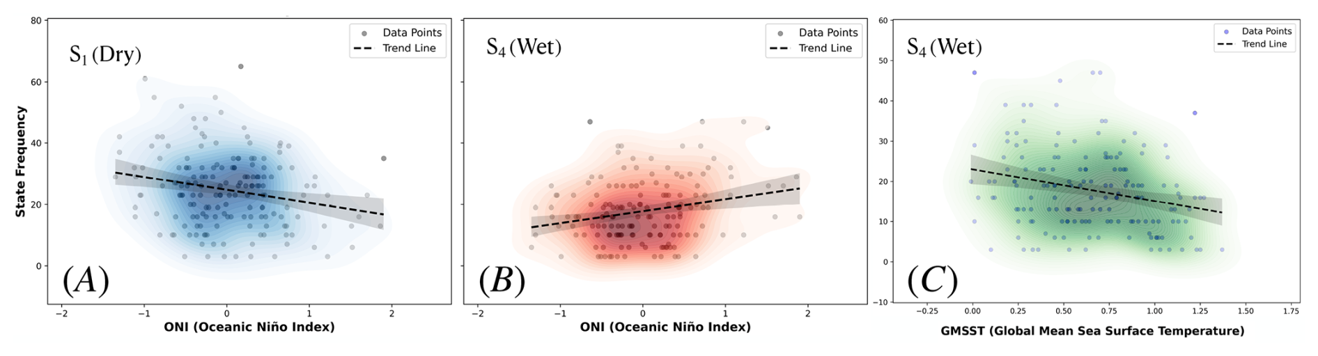
Figure 5 State–index relationships (MJJA, 1980–2022). (A) ONI vs monthly frequency of the dry state f₁; (B) ONI vs f₄; (C) GMSST vs f₄. Kernel-density contours; dashed: OLS fits with 95 % bands (descriptive only). Tail-enhanced associations motivate copula-based nonlinear dependence modelling.

3.5 Out-of-sample probabilistic simulations and verification

We evaluate the hybrid nHMM–Copula–GPD forecaster on MJJA 2022 using M=100 daily ensemble members. The nHMM is trained on 1980–2021; the 2022 state sequence is inferred by Viterbi using observed covariates.

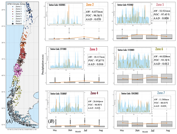
Figure 6 summarizes the DTW zone design and out-of-sample skill. Panel (A) shows the seven DTW zones with medoids marked by stars. Panel (B) shows, for six medoids (Zone 1 excluded: negligible MJJA totals in the hyperarid far north), monthly boxplots of 2022 predictive distributions (100 daily draws per day) with observed monthly means in orange; insets show daily ensembles versus observations. Ensembles reproduce the seasonal cycle and precipitation intermittency; spreads are smaller in the arid north and larger (and well-centered) in the storm-dominated south, consistent with climatological variance gradients.

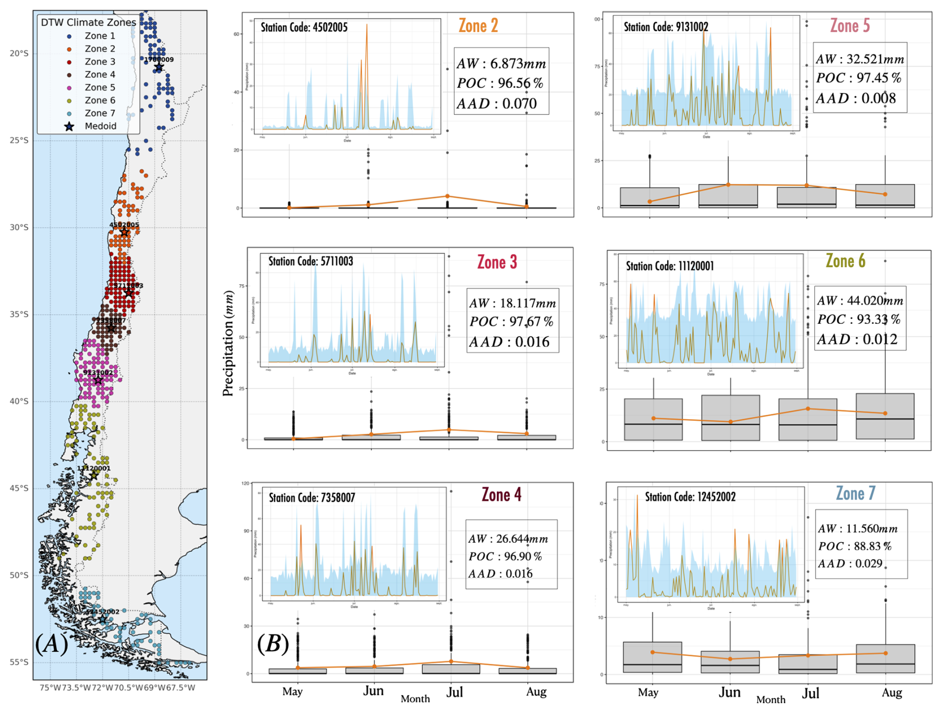
Figure 6 DTW climate zones and out-of-sample MJJA 2022 simulations. (A) Seven DTW-based climate zones (medoids: stars). (B) Monthly boxplots of MJJA 2022 predictive distributions (100 daily draws) overlaid with observed monthly means (orange). Insets: daily ensembles vs observations. Training: 1980–2021; 2022 state sequence inferred via Viterbi.

Table 6 reports interval-based metrics for MJJA 2022. Average Width (AW) increases monotonically from 6.9 mm in Zone 2 to 44.0 mm in Zone 6, reflecting the meridional gradient in climatological precipitation variance. Coverage (POC) is close to or above the nominal 90 % in all zones (88.8 %–97.7 %), confirming well-calibrated prediction intervals. Asymmetry degree (AAD) is small throughout (≤0.07), with mild right-skew in Zone 2 corresponding to occasional outlier events in the arid regime.

3.5.1 Proper scores, event-based skill, and gain from the vine-copula layer

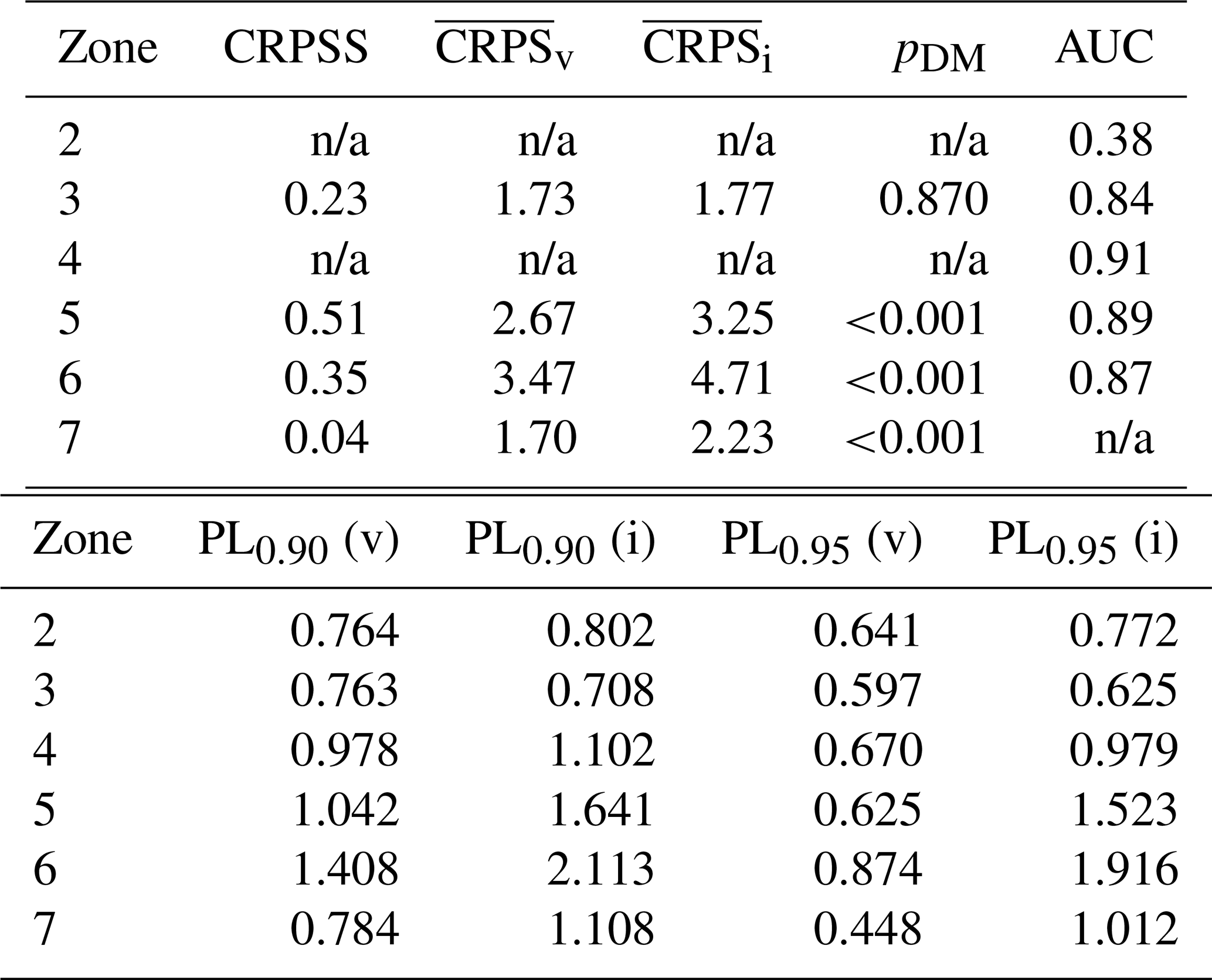
Table 7 presents the core verification results. In the rainfall-active zones (5 and 6), CRPSS reaches 0.51 and 0.35 respectively, indicating substantial improvement over the climatological benchmark; the vine-copula layer is highly significant (Diebold–Mariano p<0.001, HAC-adjusted) and reduces mean areal CRPS by 18 % (Zone 5) and 26 % (Zone 6) relative to the conditionally independent baseline. The area under the receiver operating characteristic curve (AUC) for 25 mm exceedance events reaches 0.89 and 0.87, confirming strong discrimination. Pinball losses at $\mathit{\tau }\in \mathit{\{}\mathrm{0.90},\mathrm{0.95}\mathit{\}}$ are consistently lower for the vine model, indicating that the skill gain extends to the upper quantiles most relevant for hydrological risk. Zone 3 shows a positive CRPSS of 0.23 but the vine layer is not significant (p_DM=0.87), suggesting that the copula improves the CRPS through marginal calibration rather than dependence modelling. Zone 7 (Zone covering the austral fjord region south of ≈ 45° S) shows a modest but significant CRPSS of 0.04 (p_DM<0.001); AUC could not be computed due to insufficient 25 mm exceedance events during the 2022 evaluation season.

For Zones 2 and 4, the areal-CRPS and CRPSS values are reported as not applicable (n/a) in Table 7. Zone 2 spans the Atacama and Coquimbo desert transition zone (approximately 25–30° S); precipitation is infrequent and concentrated in a small number of convective or orographic events, resulting in near-zero daily totals across the station network. Zone 4 covers the semi-arid Mediterranean transition of central Chile (approximately 33–38° S, including the pre-cordillera of O'Higgins, Maule, and northern Bío-Bío), a region with high within-zone precipitation variability driven by strong orographic gradients between coastal stations receiving a few hundred millimetres per year and Andean stations receiving several times more. Under both scenarios, the computation of a zone-wide areal mean precipitation as the scoring target amplifies two distinct numerical problems: in Zone 2, the vine ensemble occasionally generates positive draws even on days when observations are universally zero, so a single such draw inflates the areal mean and causes CRPS to diverge; in Zone 4, the extreme range of precipitation totals across the zone means that rare large draws at high-elevation Andean stations – plausible given the GPD shape $\widehat{\mathit{\xi }}=\mathrm{0.921}$ fitted for State 1 at the Zone 4 medoid, the highest shape estimate in the dataset and associated with a very small training sample (n_exc=34) – can dominate the areal mean for that state even though they occur on days when lower-lying stations record near-zero totals. In both cases, the interval-based diagnostics in Table 6 (which operate at the medoid level rather than across the full heterogeneous zone) are more appropriate and show well-calibrated performance (POC ≈97 %, AAD ≤0.07). These results collectively indicate that zone-level areal scoring is not a valid evaluation tool in regions where within-zone precipitation heterogeneity is extreme, and that the framework requires dedicated treatments – including stratified or weighted areal averages and refined zero-inflation marginals – before it can be applied in semi-arid and orographically heterogeneous zones.

Table 6 Uncertainty metrics at medoids, MJJA 2022. M=100 daily draws. AW: Average Width (mm) of central 90 % prediction interval; POC: empirical coverage (%); 95 % CI from B=500 block bootstraps; AAD: Average Asymmetry Degree. Zone 1 excluded (hyperarid far north, negligible MJJA totals).

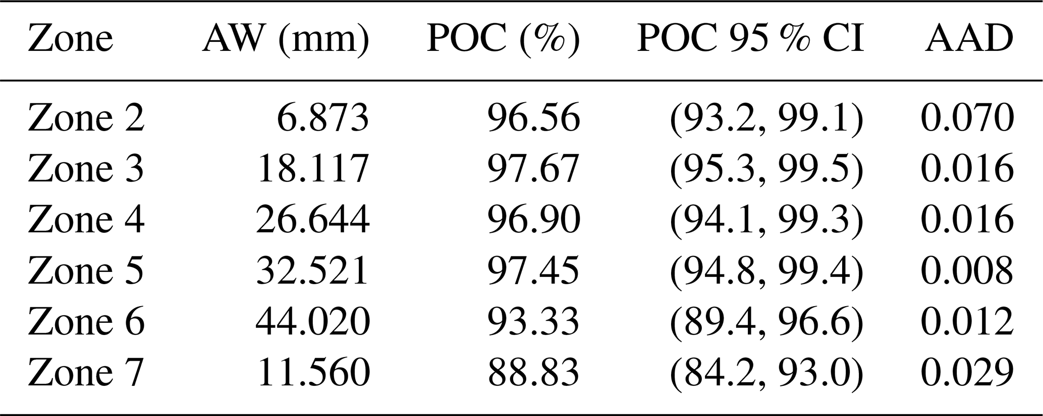
Table 7 Verification summary at zone medoids, MJJA 2022. CRPSS: CRPS Skill Score (positive = better than climatology). ${\stackrel{\mathrm{‾}}{\mathrm{CRPS}}}_{\mathrm{v}}$ and ${\stackrel{\mathrm{‾}}{\mathrm{CRPS}}}_{\mathrm{i}}$: mean areal-CRPS for vine and independence baseline (mm). p_DM: Diebold–Mariano p-value (HAC one-sided; alternative: vine < indep). PL_q: pinball loss at quantile q (vine/indep). AUC: ROC AUC for the 25 mm exceedance event. n/a: areal-CRPS not interpretable due to within-zone precipitation heterogeneity (see Sect. 3.5.1); interval-based diagnostics in Table 6 are preferred for these zones.

3.5.2 Sensitivity to modelling choices

Allowing Student-t pairs in vines, varying the GPD threshold within [0.85,0.95], and changing the state count to $K\in \mathit{\{}\mathrm{4},\mathrm{6}\mathit{\}}$ leaves PIT shapes, coverage, and event skill qualitatively unchanged (Supplement S9). Student-t pairs marginally improve heavy-rain discrimination in Zones 5–6; lower GPD thresholds slightly increase over-coverage, supporting the parsimonious main specification.

3.6 Synthesis

The hybrid framework delivers: (i) an interpretable regime taxonomy with physically coherent dry ↔ wet progression and robust vertical coupling; (ii) quantified, statistically significant trends in regime persistence consistent with documented megadrought signals; and (iii) calibrated, sharp probabilistic forecasts with significant vine-layer improvements in the rainfall-active southern zones, robust interval calibration across all zones, and well-understood limitations in semi-arid and orographically heterogeneous regions.

4 Discussion and Conclusions

This work develops and validates a hierarchical probabilistic framework for austral-winter (MJJA) precipitation in Chile, coupling a covariate-driven nHMM with DTW-based climatic zoning and state-conditioned Regular Vine copulas augmented by GPD tails. The architecture explicitly separates temporal regime dynamics from spatial residual dependence, overcoming the conditional-independence limitation of classical HMM applications to rainfall.

4.1 Summary of scientific contributions

Five hidden regimes organize MJJA precipitation along a coherent dry–wet spectrum with physically interpretable circulation signatures: ridge–high couplets with weakened westerlies in dry anticyclonic states, and trough–low couplets with intensified zonal jets in wet cyclonic states (Sect. 3.2). Regime persistence and connectivity are quantified from 1980–2022, revealing a statistically significant decline in wet-state self-transitions (≈0.34 % yr⁻¹; 95 % CI: [0.21, 0.47] % yr⁻¹), consistent with documented drying signatures in central Chile and the negative trend in S₄ associated with rising GMSST. GPD shape parameters range from bounded tails ($\widehat{\mathit{\xi }}<\mathrm{0}$, anticyclonic states) to heavy tails ($\widehat{\mathit{\xi }}>\mathrm{0}$, frontal states), with statistically robust differences confirmed by parametric bootstrap CIs (Table 2). Out-of-sample probabilistic skill is established in the rainfall-active zones: POC is close to nominal (89–98 %), interval widths increase meridionally as expected, AAD is small (≤0.07), CRPSS is positive in all zones with interpretable scores (Zones 3, 5, 6, 7), and the vine-copula layer yields statistically significant improvements over the independence baseline in the two wettest zones (p_DM<0.001). Limitations in Zones 2 and 4 are real and explained by within-zone precipitation heterogeneity rather than methodological failure; interval-based diagnostics confirm adequate calibration at the medoid level.

4.2 Relation to prior work and novelty

The novelty lies in the explicit integration of covariate-driven regime transitions, DTW-based zoning that respects temporal asynchronies, and state-conditioned high-dimensional R-vines with GPD tail augmentation for daily totals – a combination not previously assembled in the literature. This design preserves regime-physics interpretability while achieving multivariate coherence and extreme-aware behaviour at daily scales, capabilities difficult to obtain within a single monolithic spatiotemporal likelihood for q=462 sites.

4.3 Hydroclimatic implications

The detected decrease in S₄→S₄ persistence implies shorter residence times in wet, cyclone-dominated states during MJJA, directly translating into reduced winter accumulation and increasing hydroclimatic stress downstream (streamflow, snowpack, groundwater recharge). The regime classification provides a physically grounded pathway from seasonal predictors (ENSO indices, dynamical fields) to spatially consistent precipitation ensembles – through the state-transition kernel and the copula-GPD simulator – suitable for risk-aware hydroclimate operations including reservoir rule-curve testing, drought early-warning, and flood preparedness.

4.4 Limitations and pathways for improvement

The most pressing limitation is the inadequacy of zone-level areal-CRPS in climatically heterogeneous zones (2 and 4). The solution is threefold: replace the uniform areal average by an orographically weighted average; implement dedicated zero-inflated marginals for stations with very high dry-day frequencies; and apply stratified validation (separately for coastal and Andean sub-domains) before summarizing at the zone level. These modifications would not change the fundamental framework architecture but would extend its applicability to Chile's most climatically complex zones.

Other limitations include Viterbi-induced state-assignment error that can propagate to the copula layer; within-state nonstationarity that is not explicitly captured; and the modular estimation strategy that assumes conditional spatial independence during EM, though the hierarchical design repairs this in a principled and diagnostically verified manner. Future work should explore hierarchical Bayesian formulations that integrate regime, vine, and tail components with shared priors; regime-aware multivariate fields for compound-risk analysis; and assimilation of sub-seasonal dynamical predictors (MJO diagnostics, RCM output, VIMF forecasts) as transition-model covariates.

4.5 Concluding remarks

By disentangling large-scale regime dynamics from residual spatial dependence and explicitly accounting for extremes, the nHMM–DTW–vine–GPD framework delivers meteorologically coherent regimes, quantified changes in regime persistence consistent with observed megadrought trends, and calibrated, sharp probabilistic forecasts in the rainfall-active zones of Chile. The approach reconciles physical insight with statistical parsimony and computational tractability at continental scale, offering a transferable template for probabilistic hydroclimate modelling in Chile and other mountainous, hydroclimatically heterogeneous regions, with clearly specified conditions for its applicability in arid and orographically complex environments.