The ability of LSTM to model snowmelt versus rainfall generated floods

One of the most important skills of hydrological models is to simulate timing and magnitude of flood events. Long Short-Term Memory (LSTM) networks are currently among the most successful models for streamflow and flood prediction over large regions. In snow-influenced catchments, which typically comprise a minority in large-scale studies, floods are generated by two distinctly different processes, snowmelt and rainfall. The applicability of hydrological models in such regions is therefore dependent on their ability to represent both types of floods. Nevertheless, flood evaluations of LSTM taking different flood-generating processes into account are currently lacking. This study fills this gap by evaluating the ability of LSTM to model flood peak characteristics separately for snowmelt and rainfall generated floods. The trained LSTM model successfully simulated streamflow time series across the 103 evaluated catchments, with average NSE of 0.84 and average KGE of 0.86 over the unseen evaluation period. LSTM exhibited better performance in the majority of the catchments in terms of flood peak timing and magnitude for both rainfall and snowmelt generated floods when compared to the operational hydrological model in the region (HBV) used as a benchmark. LSTM had a 27 pp higher percentage of correctly simulated peak days for rainfall generated floods as compared to snowmelt generated floods, similar to what was found for HBV (29 pp). LSTM's ability to simulate flood peak magnitudes was similar for the different flood types, with percent errors within 20 % for close to half of the events. False alarm rate and probability of detection results were similar for snowmelt and rainfall generated events, both slightly better than those of mixed events. LSTM outperformed HBV in 70 %–91 % of the catchments in terms of flood peak timing and magnitude for snowmelt and rainfall generated floods. The largest improvements in flood peak magnitudes were found for rainfall generated events, in particular for catchments where HBV exhibited high (>40 %) absolute errors. Overall, our findings bring confidence that LSTM can improve hydrological services in regions subject to both snowmelt and rainfall generated floods.

1 Introduction

Reliable flood simulations are important for a range of national to local tasks, including area planning, flood and landslide forecasting, hydropower management, and climate change impact assessments. Process-based hydrological models that most commonly perform this task, have recently been challenged by deep learning Long Short-Term Memory (LSTM) networks (Hochreiter and Schmidhuber, 1997; Gers et al., 2000). Variants of LSTM networks have proven their success as rainfall-runoff models across regions, often outperforming benchmark process-based models in terms of streamflow prediction (Kratzert et al., 2018), riverine flood prediction (Frame et al., 2022) and forecasting (Nearing et al., 2024). Further, rainfall-runoff modelling by LSTM surpasses other deep learning techniques, such as traditional recurrent neural networks (Kratzert et al., 2018), feedforward neural networks (Hagen et al., 2023), and Transformer-based models (Liu et al., 2025). Unlike most process-based models that perform the best when they are locally calibrated, LSTM, being a purely data-driven model, excels when trained on big datasets of multiple catchments (Kratzert et al., 2024, 2019b). Thus, LSTM has potential to both improve and simplify hydrological services on local to global scales.

In mountainous and northern regions, it is particularly important that an applied hydrological model is able to capture effects of seasonal snow accumulation and melt on streamflow. Without physical processes or constraints explicitly implemented in the model code, a purely data-driven model needs to learn such effects solely from the training data. In LSTM, long-term dependencies between input and output time series are handled by memory cells that can represent depletion, increase and outflow of reservoirs and storages in the case of hydrological modelling (Kratzert et al., 2019a, 2018). Studies have indeed shown how LSTM cell state vectors produce temporal dynamics matching our physical understanding of snow accumulation and melt (Kratzert et al., 2018), and with good (>0.8) correlations with snow depth reanalysis products (Lees et al., 2022). Correspondingly, LSTMs have demonstrated good performance in snow-influenced regions in terms of simulating streamflow in general (Roksvåg et al., 2026; Jiang et al., 2022), and flood peaks in particular (Martel et al., 2025; Hagen et al., 2023; Anderson and Radić, 2022).

As snowmelt and rainfall generated floods are substantially different in their underlying physics and temporal dependencies of past weather, the performance of a hydrological model may differ for the two types of floods. Identifying and understanding such difference are important both for improving models and quantification of uncertainty in model simulations and forecasts. Nevertheless, to our knowledge, existing evaluations of LSTM's ability to simulate floods are performed over all identified flood events, without evaluating events generated by different processes separately. Evaluation results over all flood peaks mainly reflect the model's ability to simulate the flood type possessing the majority of the events, whereas the ability to simulate other flood types of importance is left unknown (Martel et al., 2025). This is a particular issue for regions with seasonal snow cover where floods are primarily driven by two fundamentally different processes, snowmelt and rainfall, and an applied hydrological model should be able to simulate both flood generating processes.

This study meets the abovementioned gap by investigating the ability of LSTM to simulate floods of different driving mechanisms. The main objective is to evaluate LSTM's potential for operational use in snow-influenced regions, focusing on prediction of floods dominantly generated by snowmelt and rainfall separately. The study area is the mainland of Norway, a country spanning 58–71° N that has a large variability in topography, annual precipitation amounts and seasonal snow cover. The applicability of LSTM for a given country or region depends on the performance of LSTM versus the regions' state-of-the-art operational hydrological model in terms of hydrological features that are important in that region. Accordingly, we use a national operational hydrological model as a benchmark. We meet our aim by answering the following research questions:

1. Is LSTM able to simulate streamflow series with similar or exceeding overall performance as compared to the operational model used in the region?

2. How well does LSTM simulate peak timing and magnitude of all collected floods generated by (i) snowmelt, (ii) rainfall and (iii) a mix of the two?

3. How well does LSTM simulate per-catchment peak timing and magnitude of (i) snowmelt generated floods and (ii) rainfall generated floods?

The paper is structured as follows: In Sect. 2 the data underlying the analyses are described, followed by methods explaining the applied LSTM and HBV model, flood event detection and classification, and the applied model evaluation metrics. Section 3 presents the results, which are further discussed in Sect. 4 before conclusions are drawn in Sect. 5.

2 Data and methods

2.1 Hydroclimatology and floods in Norway

Norway exhibits a high heterogeneity in hydroclimatological conditions (Dyrrdal et al., 2025). The country spans 58 to 71° N along the west side of the Scandinavian peninsula with coastline comprising the southern, western and northern border, and with the Scandinavian mountain range running southwest to northeast. Annual precipitation amounts range from above 6000 mm in the west due to the combination of prevailing westerly winds from the Atlantic and orographic effects, to below 300 mm towards central-eastern and northeastern parts of the country. The geographical pattern of annual runoff reflects to a large degree that of annual precipitation. Annual temperatures varies from −9.5 to 9.5 °C, with the warmest areas along the southern and western coastline, and coldest in the inland high altitudes or latitudes. Although the snow season and volumes vary considerably across Norway following the heterogeneity of temperature and precipitation, most of the country has temperatures above 0 °C during summer and below 0 °C and snowfall during winter.

Floods in Norway are mainly generated by rainfall and snowmelt or a combination of the two (Berghuijs et al., 2019; Vormoor et al., 2016). Whereas extreme rainfall events typically occur in summer or autumn, snowmelt typically peaks in spring or early summer. Generally, the largest floods are dominantly generated by rainfall in southern and western regions, and by snowmelt in central-eastern and northern regions.

2.2 Discharge data and catchment attributes

Daily discharge data used to train the LSTM network stemmed from 200 streamflow gauging stations of the Norwegian Water Resources and Energy Directorate (NVE) hydrometric observation network in Norway (Fig. 1). Of those stations, model evaluation was performed over the 103 stations used by the operational model, which serves as a benchmark (ref. Sect. 2.5). Each day in the observed daily discharge series is divided at midnight Central European Time (CET).

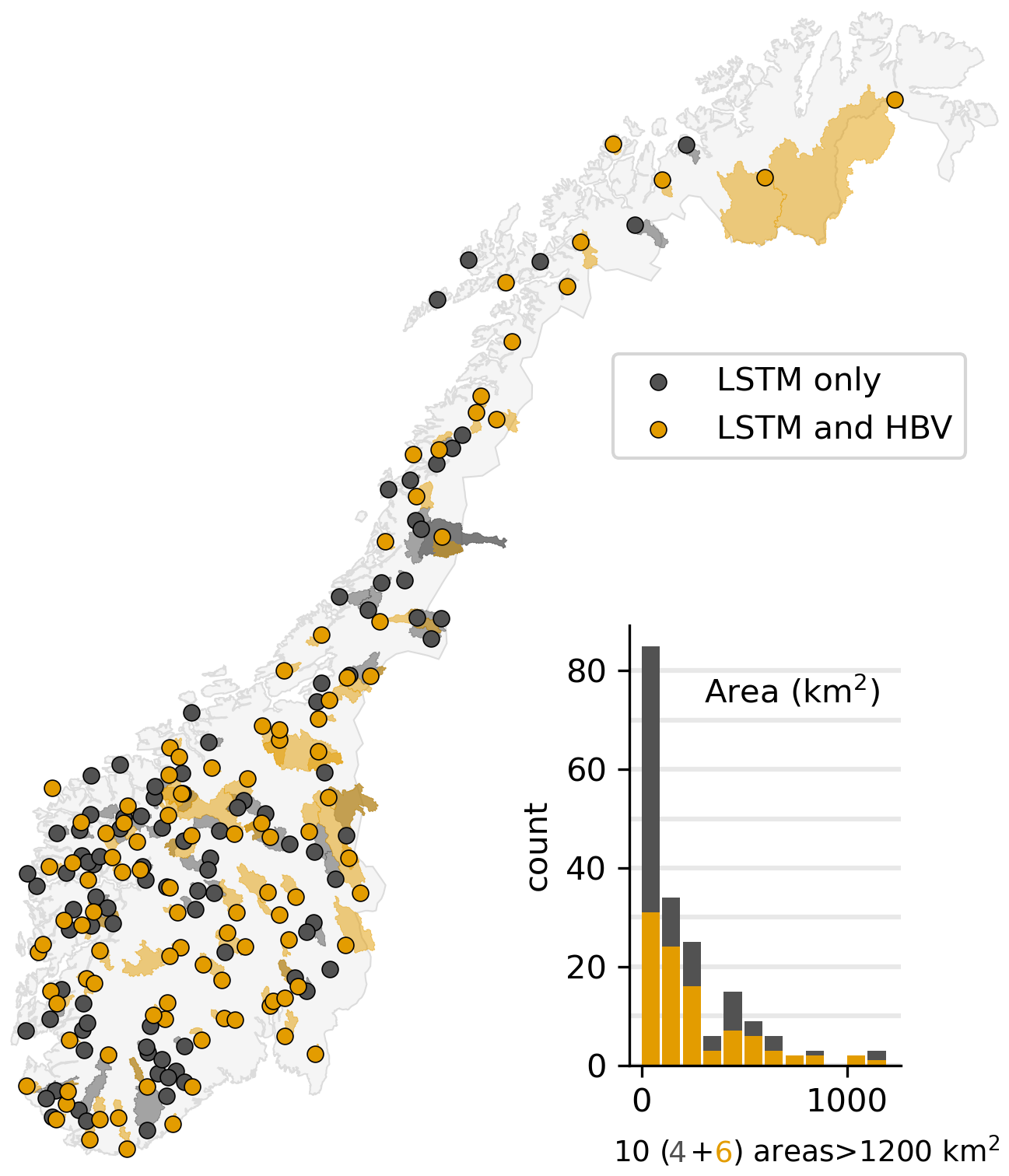
Figure 1 Locations and catchments of the streamflow gauging stations, and histogram of catchment areas. All 200 catchments (both yellow and dark grey) were used to train the LSTM model, whereas yellow represents the 103 catchments where both LSTM and HBV have simulations (used for model evaluation). Catchment polygons from GeoNorge (2026a).

The gauging stations were selected from an existing dataset that has been thoroughly quality controlled for flood analyses (530 stations; Engeland et al., 2016). Requirements during that selection included: The stations should not have problems with ice jams or supercritical flow during floods, they should have satisfactory rating curves and measurement conditions during floods, and they should not have homogeneity breaks for streamflow and floods that stemmed from changes in the measurements or quality control. Of the 530 stations, we selected the active stations unaffected by regulations. The original unit of m³ s⁻¹ was changed to mm d⁻¹ by normalising the streamflow values by the catchment areas. Catchment areas represented in the dataset range 0.58 up to 14 000 km². However, most areas are less than 300 km², which was expected due to the requirement of near-natural flow in a country heavily affected by hydropower.

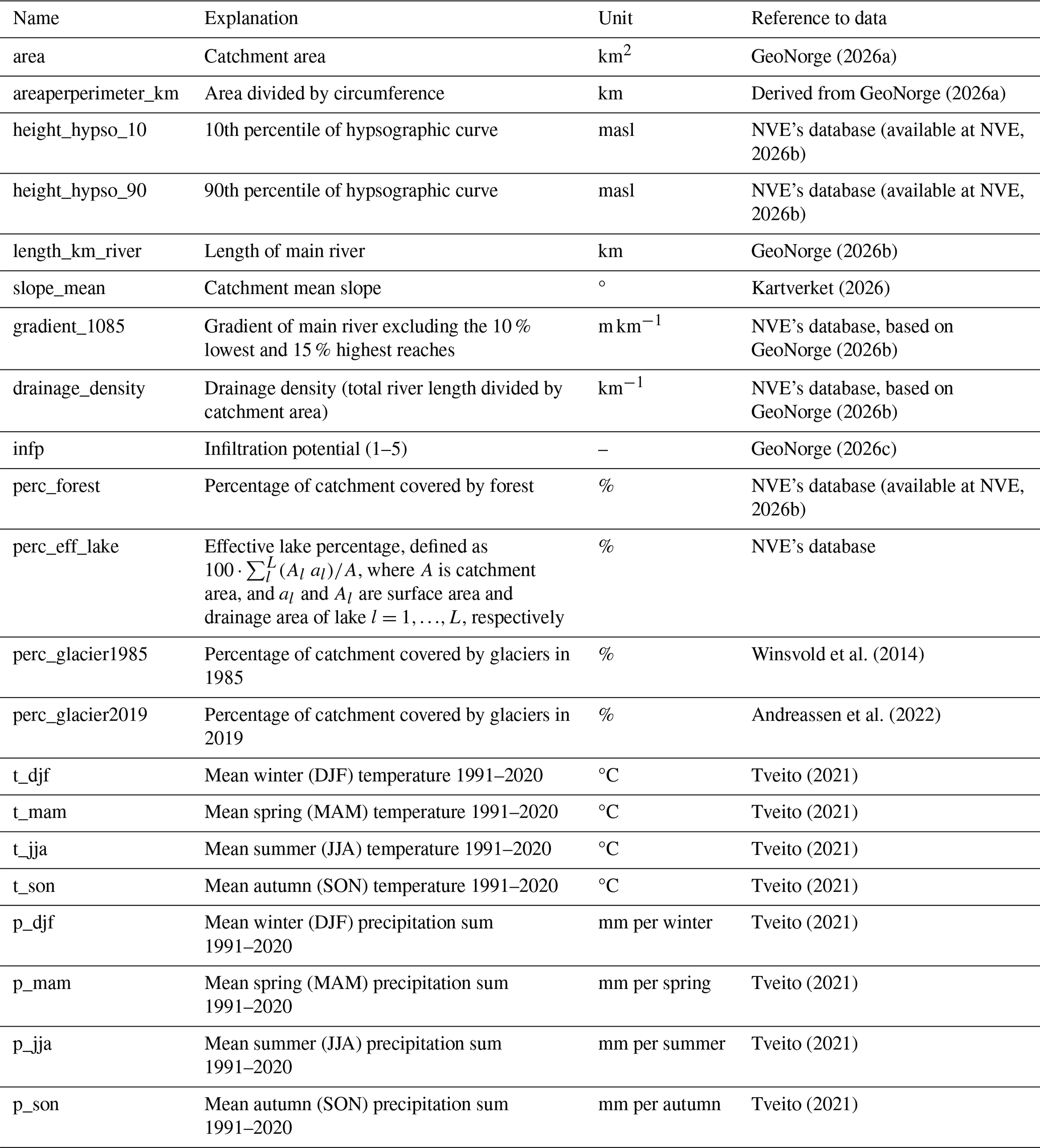
Table 1 lists the catchment attributes selected for the training of the LSTM model. The 21 catchment attributes were selected to represent the variability of geometric, physiographic and climatological characteristics important for streamflow, hydrological regimes and floods. There is a large degree of overlap between our selection and attributes that have previously been selected for regional flood frequency models in Norway (Engeland et al., 2020; Barna et al., 2023a). Most of the catchments are influenced by seasonal snow. Of all the 200 catchments, 95 % have average winter (DJF) temperatures below 0 °C (range −13 to 3 °C), whereas average summer (JJA) temperatures are all positive, ranging 6 to 16 °C. Several of the catchments are also partly covered by glaciers. Specifically, 21 (12) of the 200 catchments have more than 3 % (10 %) of their catchment area covered by glaciers in 2019.

GeoNorge (2026a)GeoNorge (2026a)(available at NVE, 2026b)(available at NVE, 2026b)GeoNorge (2026b)Kartverket (2026)GeoNorge (2026b)GeoNorge (2026b)GeoNorge (2026c)(available at NVE, 2026b)Winsvold et al. (2014)Andreassen et al. (2022)Tveito (2021)Tveito (2021)Tveito (2021)Tveito (2021)Tveito (2021)Tveito (2021)Tveito (2021)Tveito (2021)

Table 1 Catchment attribute names, explanations, units and references to data.

2.3 Gridded hydrometeorological data

Daily precipitation sum (mm) and mean daily temperature (°C) from the meteorological dataset SeNorge_2018 (Lussana et al., 2019) was used to produce the dynamical forcing for LSTM (Sect. 2.4). Flood event classification (Sect. 2.6) was based on the same precipitation data, as well as daily snowmelt (mm) estimates simulated by the SeNorge snow model v.1.1.1 (Saloranta, 2016) that uses SeNorge_2018 gridded daily precipitation sum and mean temperature as input. Both SeNorge_2018 and the snowmelt dataset are available from 1957 to present at a daily time step (07:00–07:00 CET). They are gridded products with a spatial resolution of 1×1 km², covering the whole of Norway as well as neighbouring regions. The SeNorge_2018 dataset is generated by statistical interpolation of in situ precipitation and temperature observations. The SeNorge snow model used for classifying flood events simulates snowmelt by a degree-day approach augmented with synthetic incoming daily solar irradiance defined as a function of latitude and time of the year.

From the daily gridded variables precipitation sum and mean temperature, the following daily time series were prepared at the catchment level for LSTM modelling:

• prec (mm d⁻¹): Spatially averaged daily precipitation sum

• temp_ave (°C): Spatially averaged daily mean temperature

• temp_min (°C): The minimum value of all catchment grid cells' daily mean temperature

• temp_max (°C): The maximum value of all catchment grid cells' daily mean temperature

Further, based on daily gridded precipitation sum and snowmelt, the following time series were prepared at the catchment level to identify flood generating processes:

• snowmelt (mm d⁻¹): Spatially averaged daily snowmelt

• rainfall (mm d⁻¹): Spatially averaged daily rainfall sum. For each grid cell, the daily rainfall sum was defined as the daily precipitation sum if the daily mean temperature was equal or larger than 0.5 °C, and 0 mm d⁻¹ otherwise.

2.4 Long Short-Term Memory networks

Recurrent neural networks operate on time series data by processing a d-dimensional input sequence $\mathit{\{}{x}_{\mathrm{t}}\in {\mathbb{R}}^d:t=\mathrm{1},\mathrm{2},\mathrm{\dots },T\mathit{\}}$ and generating a p-dimensional output sequence $\mathit{\{}{y}_{\mathrm{t}}\in {\mathbb{R}}^p:t=\mathrm{1},\mathrm{2},\mathrm{\dots },T\mathit{\}}$ through recursive computations. At each time step t, the network updates its internal state and produces an output according to:

$$\begin{array}{}\text{(1)}& h_{\mathrm{t}}=f(x_{\mathrm{t}},h_{\mathrm{t}-\mathrm{1}}),y_{\mathrm{t}}=g\left(h_{\mathrm{t}}\right),\end{array}$$

where h_t∈ℝ^k represents the k-dimensional hidden state that encodes information from previous time steps, while f and g are parametrised functions that define the network's dynamics and output mapping, respectively.

LSTM networks implement a sophisticated version of the state update function f that allows the LSTM to selectively retain or forget information over long sequences, mitigating the vanishing gradient problem that affects traditional recurrent neural networks (Gers et al., 2000). In the context of streamflow prediction, this long-term memory capability enables the model to represent snowpack dynamics by retaining information about precipitation and temperature conditions during winter months, then utilizing this stored information to predict the timing and magnitude of snowmelt-driven streamflow in spring and summer (Lees et al., 2022). For a detailed decomposition of the LSTM state update function, see Kratzert et al. (2018).

To predict streamflow at day t, the model requires an input sequence $x_{(\mathrm{t}-m):\mathrm{t}}=\mathit{\{}{x}_{\mathit{\tau }}:\mathit{\tau }=t-m,t-m+\mathrm{1},\mathrm{\dots },t\mathit{\}}$ of length m+1, which is processed through the LSTM to produce a corresponding output sequence $y_{(\mathrm{t}-m):\mathrm{t}}$. The output, ${\widehat{q}}_{\mathrm{t}}$, the streamflow at day t, is obtained by taking the final element of this output sequence, i.e., ${\widehat{q}}_{\mathrm{t}}=y_{\mathrm{t}}$. To simulate streamflow for the next timestep, the input window is shifted one time step forward at each prediction.

We employed LSTM as a lumped rainfall-runoff model using the cudalstm architecture from the neuralhydrology package (Kratzert et al., 2022), a Python library containing a collection of LSTM-based models for hydrological modeling built on the PyTorch framework. The cudalstm model provides an efficient GPU-accelerated implementation of the LSTM architecture described here.

The LSTM model was trained using the 15 hydrological years 1 September 2009–31 August 2024, employing the catchment-averaged Nash-Sutcliffe efficiency (NSE) as our loss function, in line with Kratzert et al. (2019b). Details of our LSTM training and hyperparameter tuning using a 5-fold cross-validation (CV) are provided in Appendix A. The model was trained using four meteorological input time series for each catchment: catchment-averaged daily precipitation sum (mm d⁻¹), catchment-averaged mean daily temperature (°C), catchment-minimum mean daily temperature (°C), and catchment-maximum mean daily temperature (°C). In addition to these dynamic inputs, the model incorporated 21 static catchment attributes as listed in Table 1. Following best practice (Kratzert et al., 2024, 2019b), a single LSTM model was trained across all catchments, enabling the model to learn general hydrological relationships from the diverse set of catchments.

2.5 Benchmark model

The Hydrologiska Byråns Vattenbalansavdelning (HBV) model (Bergström, 1976) is a widely used precipitation-runoff model, in particularly in the Nordic countries (Addor and Melsen, 2019; Seibert and Bergström, 2022). In Norway, a version of the HBV model with a daily temporal resolution is used operationally by NVE, for national flood warning services, quality control of streamflow observations, and energy prognosis among others (Lawrence et al., 2009; Ruan and Langsholt, 2017). For this reason, we chose the operational HBV model for benchmarking our results. Catchment-by-catchment calibration of 12 model parameters were performed using Nash-Sutcliffe efficiency (NSE) as a loss function (for calibration details, see Appendix B). The operational HBV model are currently used for 145 reference catchments with long data series of good quality and limited influence of regulations, and representative for different geographical regions in Norway (Ruan and Langsholt, 2017). We performed all model evaluations for the 103 reference catchments that overlapped with the catchments used for training LSTM (Fig. 1).

2.6 Detection of flood events and flood generating processes

Flood events were selected from the observational time series based on a peak over threshold (POT) approach, following the methods described in Vormoor et al. (2016). Daily streamflow values exceeding the 98th percentile calculated from the 30-year period 1 September 1994–31 August 2024 were used to identify the flood peaks. To ensure independence between flood events, only the maximum streamflow value was selected within a catchment-specific time window, using the python library pyextremes (Bocharov, 2023). This time window was set to twice the normal flood duration (NFD), which is defined as the sum of concentration time plus recession time of the largest flood events. The full description of the estimation of NFD is provided in Vormoor et al. (2016). In general, a concentration time of 2–3 d was found for all catchments subject to an HBV modelling experiment inputting twice the annual rainfall over a 2 d period to a fully drained catchment. The median of two days was then chosen for all catchments. Recession times were estimated using the methods described in Skaugen and Onof (2014), which fit a recession curve to the largest flood events from the observational data series. Our 200 gauging stations have NDF spanning 2 to 45 d.

Flood generating process (FGP) was defined for each event based on the relative contribution of rainfall and snowmelt to the flood, based on the approach in Vormoor et al. (2015). We selected this approach from the range of available flood classification schemes (Tarasova et al., 2019) because it provides a simple yet effective distinction between rainfall and snowmelt generated floods and has been successfully applied in studies conducted within our region (Yan et al., 2023; Vormoor et al., 2016, 2015). To account for antecedent conditions, the contribution to a specific flood was computed as the sum of rainfall and snowmelt in a catchment-specific time window prior to, and including, the flood peak day. This time window was set as the catchment-specific recession times as defined above. Figure 2 shows the average fractional contribution of rainfall to flood events, reflecting the dominant flood generating process (FGP) in each catchment. Using the thresholds proposed by Vormoor et al. (2015), all flood events were classified into snowmelt generated events, rainfall generated events and mixed events depending on whether more than two thirds of the contribution stemmed from snowmelt, rainfall or neither, respectively. The distribution of all flood events' fractional rainfall contribution, along with the flood type classification thresholds, is shown in Fig. C3. The figure further shows two alternative pairs of classification thresholds used to assess the results' sensitivity to the chosen thresholds.

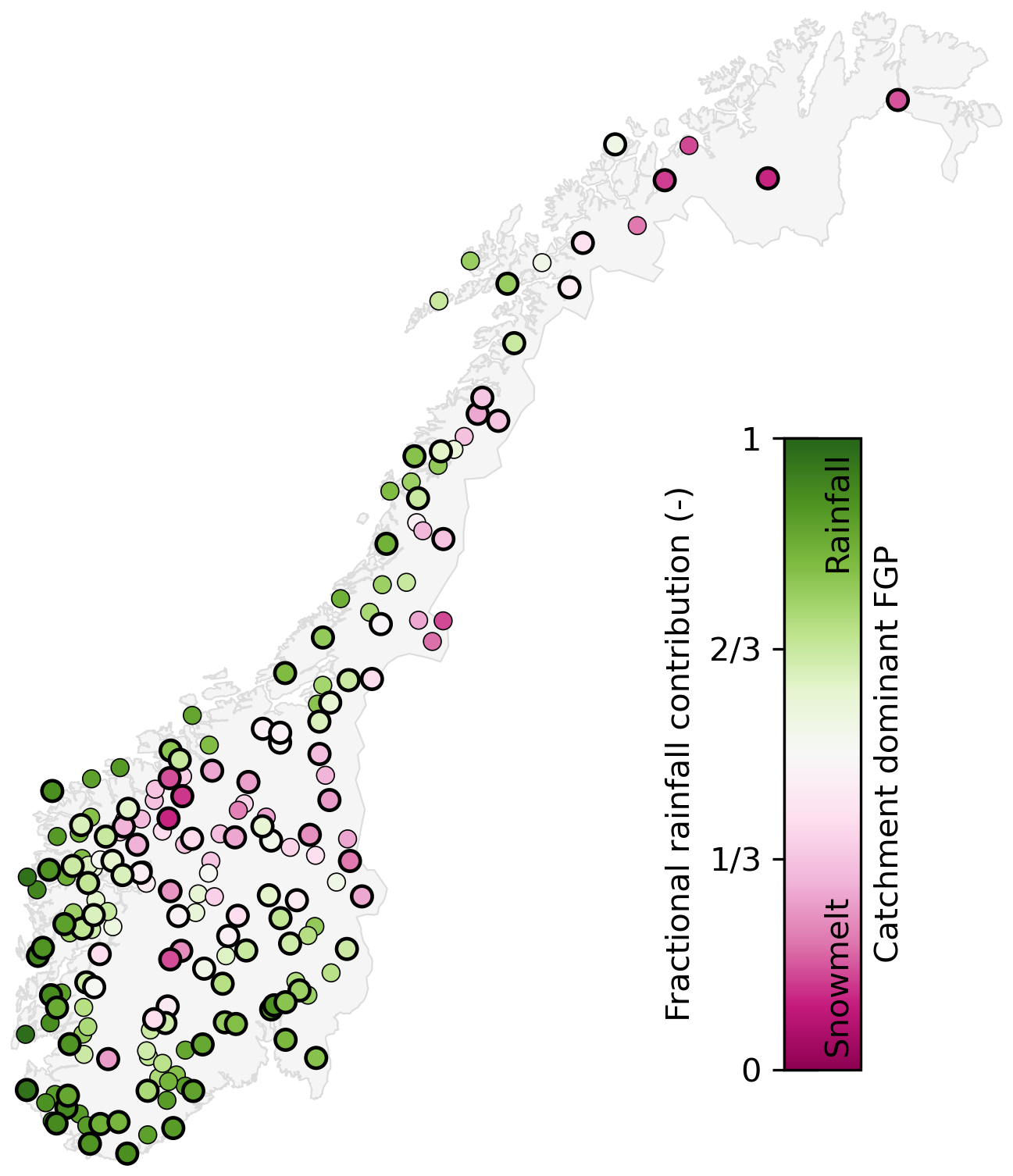
Figure 2 Average fractional rainfall (i.e. proportion of total) contribution to all observed flood events in the period 1 September 1994–31 August 2024, and its relation to the catchment dominant flood generating process (FGP). Dark pink (green) dots represent catchments with snowmelt (rainfall) as their dominant FGP, whereas near-white dots represent catchments with similar average contributions from rainfall and snowmelt. All 200 catchments used for training the LSTM are shown, with thicker circles representing the 103 catchments used for model evaluation.

2.7 Model evaluation

Both LSTM and our benchmark HBV model were evaluated using a period unseen during model training/calibration, i.e. 15 hydrological years comprising 1 September 1994–31 August 2009. Early 1990s is typically considered the start of thoroughly quality-controlled rating curves for a large proportion of the Norwegian streamflow gauging stations. We did not want the models to suffer from changes in the water balance from the calibration period to the evaluation period due to changes in the precipitation measuring network. To assess whether this was the case, we computed the runoff coefficient, defined as the ratio of streamflow to precipitation, for the two periods. For most catchments, the runoff coefficients were similar between the two periods (Fig. C1). However, for four (13) catchments, a 30 % (20 %) change in the runoff coefficient from training to evaluation period was detected, which might have had an influence on the model performance results. Negative discharge values in the LSTM simulations were truncated to zero prior to the evaluation, and simulated series for each catchment were masked by data gaps existing in the observed series.

We evaluated model performance in terms of (i) per-catchment overall performance, (ii) descriptive statistics over all collected peaks of each flood type, and (iii) per-catchment flood peak performance of each flood type. In terms of (i), we assessed the fit between observed and simulated streamflow across the evaluation period for each catchment using Nash-Sutcliffe efficiency (NSE), the updated Kling-Gupta efficiency (KGE; Kling et al., 2012), and mean absolute error (MAE), all defined in Table 2. Additionally, we assessed the three components comprising KGE: Pearson correlation coefficient (ρ), bias ratio (β) and variability ratio (γ). The two latter are defined as:

$$\begin{array}{}\text{(2)}& \mathit{\beta }={\displaystyle \frac{\stackrel{\mathrm{‾}}{\widehat{q}}}{\stackrel{\mathrm{‾}}{q}}}\end{array}$$

and

$$\begin{array}{}\text{(3)}& \mathit{\gamma }={\displaystyle \frac{{\mathit{\sigma }}_{\widehat{q}}/\stackrel{\mathrm{‾}}{\widehat{q}}}{{\mathit{\sigma }}_q/\stackrel{\mathrm{‾}}{q}}}\end{array}$$

where $\stackrel{\mathrm{‾}}{\widehat{q}}$ is mean simulated streamflow, $\stackrel{\mathrm{‾}}{q}$ is mean observed streamflow, ${\mathit{\sigma }}_{\widehat{q}}$ is standard deviation of simulated streamflow, and σ_q is standard deviation of observed streamflow.

In step (ii), we used descriptive statistics to summarise the flood peak performance in terms of timing and magnitudes over all collected flood peaks (i.e. independent of catchment) of each flood type: snowmelt generated floods, mixed floods and rainfall generated floods. Timing was evaluated by computing the percentage of peaks of a given flood type simulated at the day of observed peak (i.e. correct timing), one day too early or too late, or more than one day too early or too late. Flood peak magnitudes were evaluated by percent errors, considering both the simulated discharge magnitude at the day of observed flood peak (PE_peak,pinned) and the simulated maximum discharge within a 2 d time window of the observed flood peak (PE_{peak,floating}). The latter allows comparison of peak magnitudes even if the model does not match the exact day of the observed peak. The definitions of these metrics are as follows. For each catchment s∈S, let n be the number of observed floods of a specific type at catchment s. Let t_j denote the timestep of the jth observed flood peak. Define $q_{s,j}:=q_{s,t_j}$ and ${\widehat{q}}_{s,j}:={\widehat{q}}_{s,t_j}$ as the observed and simulated streamflow at the jth peak, respectively. Then, PE_peak,pinned for peak j at catchment s is

$$\begin{array}{}\text{(4)}& {\text{PE}}_{\text{peak,pinned}}^{s,j}={\displaystyle \frac{{\widehat{q}}_{s,j}-q_{s,j}}{q_{s,j}}}\cdot \mathrm{100},\end{array}$$

for $j=\mathrm{1},\mathrm{\dots },n$ and s∈S. Further, defining the window $I_j=\mathit{\{}i\in Z:|i-t_j|\le \mathrm{2}\mathit{\}}$, PE_{peak,floating} is

$$\begin{array}{}\text{(5)}& {\text{PE}}_{\text{peak,floating}}^{s,j}={\displaystyle \frac{{max}_{i\in I_j}{\widehat{q}}_{s,i}-q_{s,j}}{q_{s,j}}}\cdot \mathrm{100}.\end{array}$$

Further, we computed the false alarm rate (FAR) and probability of detection (POD) of each flood type (e.g. Wu et al., 2025). FAR measures the percentage of false positives, i.e. incorrectly identified flood events by a given model, and has an optimum value at 0 %. To compute FAR, we applied the flood event selection and classification procedure described in Sect. 2.6 on the simulated streamflow series. For each detected simulated flood event, the corresponding “pinned” (i.e. exact day) and “floating” (i.e. maximum within a 2 d time window) observed streamflow value was extracted and defined as a non-flood event if the value did not exceed the 98th percentile. FAR_pinned and FAR_floating were then defined as the percent of simulated flood events that had corresponding pinned, respectively floating, observed non-flood events. POD measures to what degree a model is able to capture the observed flood events. It has an optimum at 100 %. POD_pinned and POD_floating were computed as the percent of observed flood events that had a corresponding pinned, respectively floating, simulated streamflow exceeding the 98th percentile. We compared FAR and POD results using the 98th percentile streamflow magnitudes extracted from each individual (simulated and observed) time series with results using only the observed series to define the 98th percentile streamflow magnitudes.

Table 2 Definitions of per-catchment evaluation metrics used in this study: Nash-Sutcliffe efficiency (NSE), Kling-Gupta efficiency (KGE), mean absolute error (MAE), mean absolute percentage error (MAPE_peak,pinned and MAPE_{peak,floating}) and timing error. Here q_t and ${\widehat{q}}_{\mathrm{t}}$ are observed and simulated streamflow for a specific catchment at timestep t, $\stackrel{\mathrm{‾}}{q}=\frac{\mathrm{1}}{T}{\sum }_{t=\mathrm{1}}^T{q}_{\mathrm{t}}$ is the mean observed streamflow, 𝕀(⋅) is the indicator function and $d_j={\widehat{t}}_j-t_j$ is the difference in days between the simulated and observed peak for event j $(j=\mathrm{1},\mathrm{\dots },n)$, where n is the number of observed floods of a specific type at that catchment. We used adjusted KGE such that ρ is the Pearson correlation coefficient, β is the bias ratio (Eq. 2), and γ is the variability ratio (Eq. 3), all computed over the period $t=\mathrm{1},\mathrm{\dots },T$. The quantities ${\text{PE}}_{\text{peak,floating}}^j$ and ${\text{PE}}_{\text{peak,pinned}}^j$ are defined in Eqs. (4) and (5), respectively.

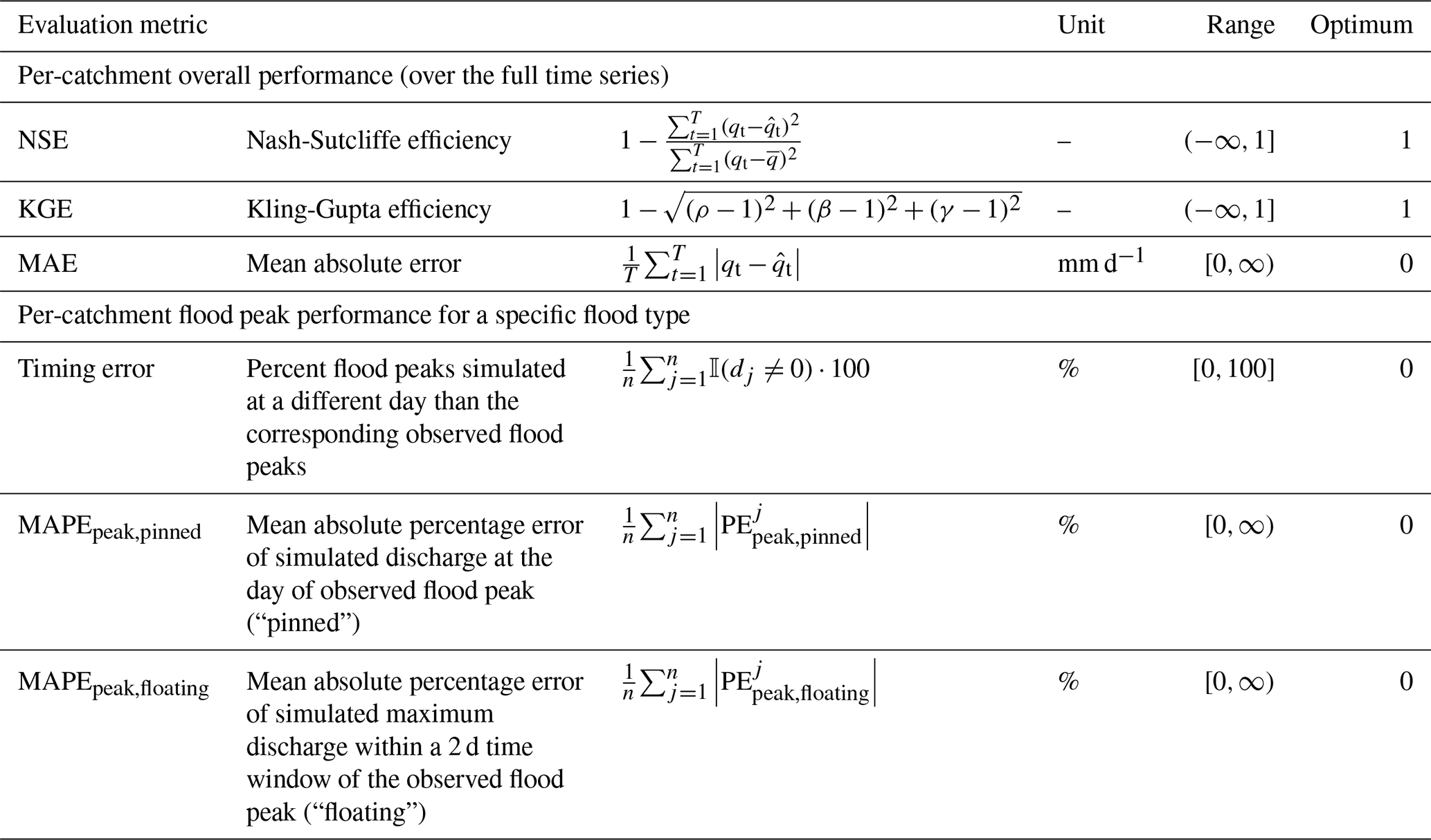
In the final evaluation step (iii), we evaluated per-catchment timing error and mean absolute percentage error of flood peaks separately for each flood type, as defined in Table 2. Timing error represents the percent of flood peaks that are simulated at a different day than the observed flood peaks. Corresponding to the definitions of PE_peak,pinned and PE_{peak,floating} above, we computed the mean absolute percentage error of flood peaks considering both pinned (MAPE_peak,pinned) and floating (MAPE_{peak,floating}) simulated peaks. The per-catchment flood peak performance metrics were only computed for catchments with minimum ten flood events of the given flood type in the evaluation period. A minimum of ten flood events during the evaluation period were found for 45 catchments for snowmelt generated floods, 60 catchments for rainfall generated floods (including 13 of the same catchments that had minimum ten snowmelt generated floods), and five catchments for mixed floods. Due to the low number of catchments with the required number of mixed flood events, the results for mixed floods are excluded from the per-catchment flood peak performance results.

3 Results

3.1 Overall model performance

The LSTM model performance in terms of NSE and KGE are shown for the evaluated catchments in Fig. 3. Importantly, all results were computed for the unseen evaluation period (ref. Sect. 2.7). Average scores were 0.84 for NSE and 0.86 for KGE, and NSE (KGE) scores exceeded 0.7 in 100 (102) catchments. The KGE components (ρ, β and γ) and MAE results are presented in Fig C2. All ρ (i.e. correlation coefficient) scores exceeded 0.83, whereof 83 % of them exceeded 0.9. A total of 82 % of the catchments had a β (i.e. bias ratio) in the range 0.9–1.1 with a similar percentage of catchments below (46 %) and above (54 %) the optimum of 1. For γ (variability ratio), 70 % of the catchments had values in the range 0.9 to 1.1, and in 82 % of the catchments the coefficient of variation was underestimated (i.e. γ<1). MAE scores ranged 0.2 to 4.2 mm d⁻¹ with a average of 1.1 mm d⁻¹.

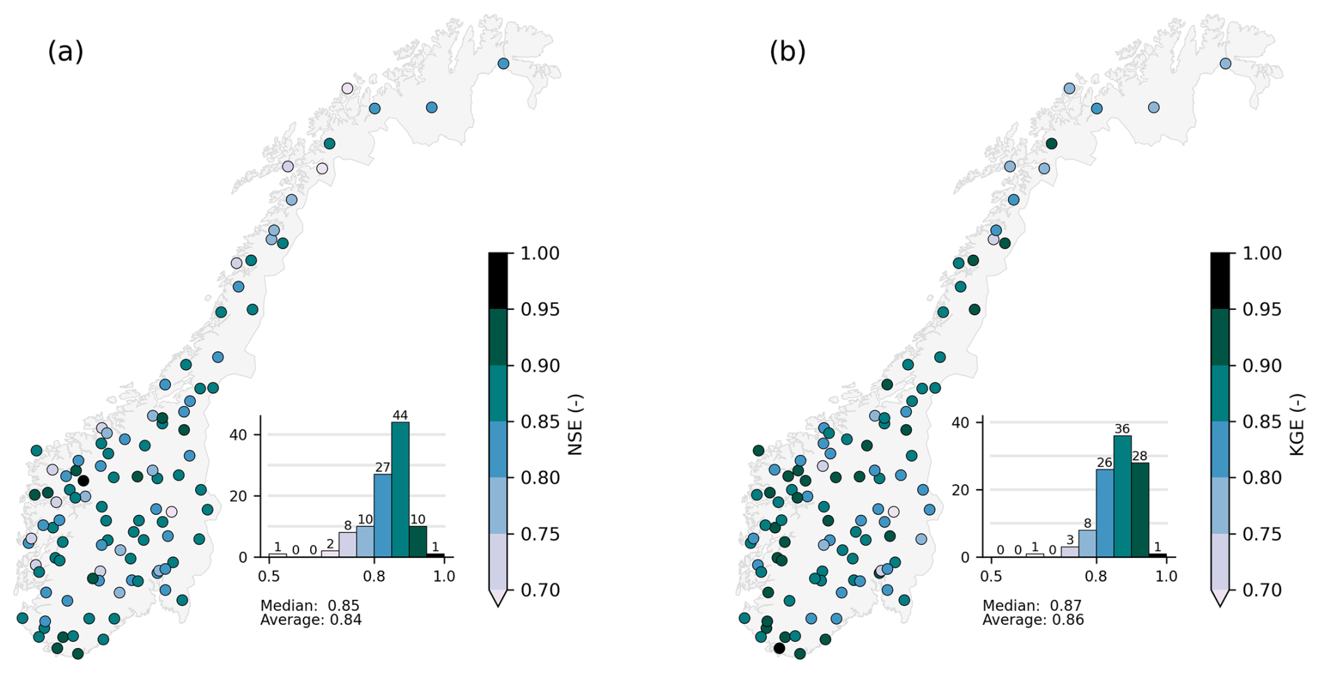
Figure 3 (a) Nash-Sutcliffe efficiency (NSE) and (b) Kling-Gupta efficiency (KGE) of LSTM for the 103 evaluated catchments.

To benchmark our results, the LSTM NSE and KGE values were compared with those of the HBV model (Fig. 4). A total of 99 catchments (96 %) had a higher NSE score for LSTM as compared to HBV, with the score difference exceeding 0.1 for 27 of the catchments. In terms of KGE, a higher LSTM score was found for 79 of the 103 catchments (77 %), with a KGE difference exceeding 0.1 for 12 catchments. One of the HBV KGE scores exceeded the corresponding LSTM scores by more than 0.1. The overweight of higher LSTM scores is reflected in the overweight of catchments above the diagonal line in Fig. 4c, d. The largest improvement in scores when comparing LSTM to HBV were found for catchments with HBV scores below 0.6. Catchments with floods predominantly generated by snowmelt (i.e. pink coloured dots) had generally higher NSE scores than catchments predominantly generated by rainfall (i.e. green coloured dots) for HBV. A similar pattern was not found for LSTM's NSE scores, nor for any of the models' KGE scores. In terms of the KGE components, LSTM had a better score for ρ in 93 %, β in 74 %, and γ in 44 % of the catchments. In all but three catchments, mean absolute errors were lower (i.e. better) for LSTM as compared to HBV.

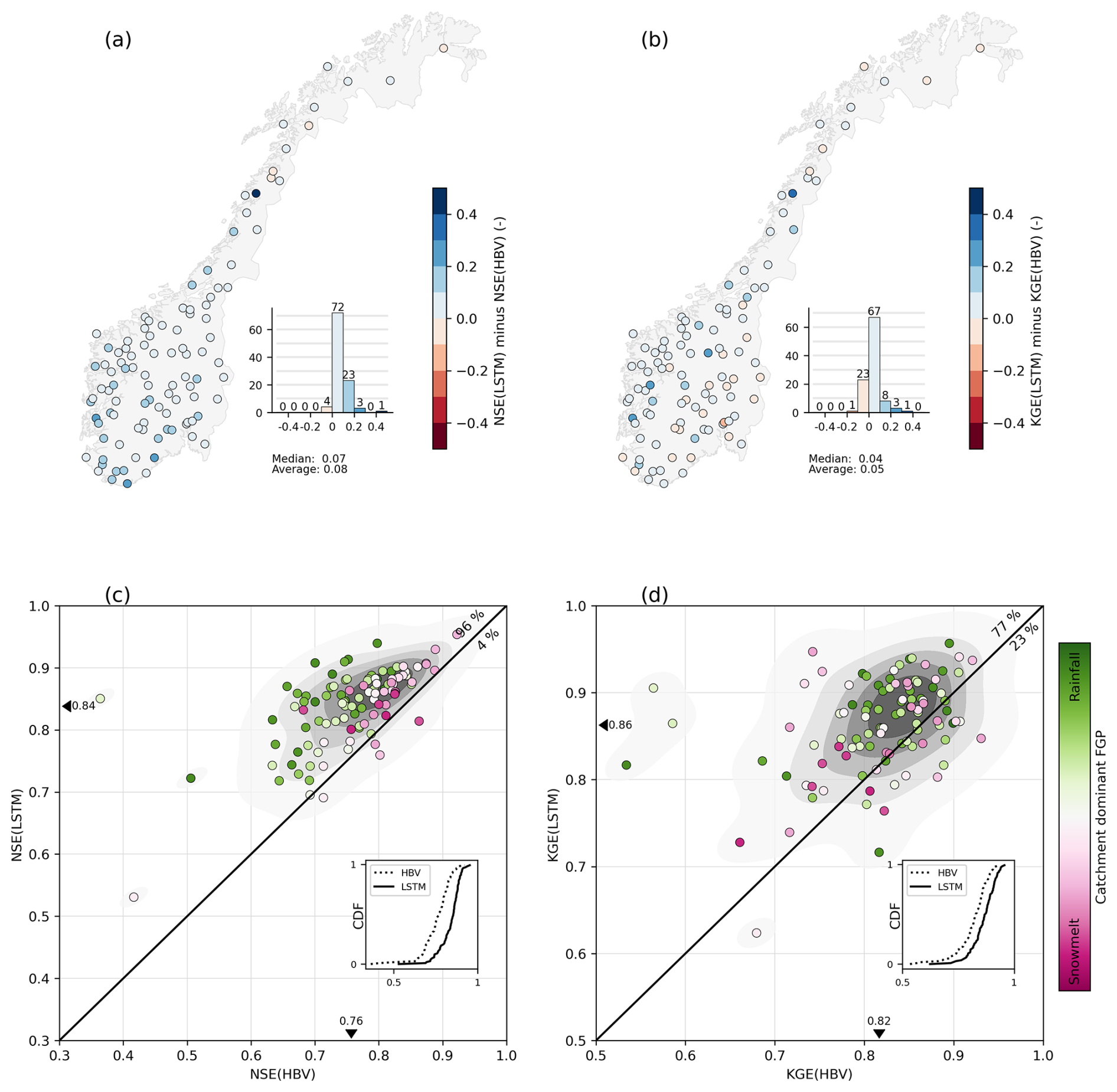
Figure 4 Difference between LSTM and HBV in (a) NSE and (b) KGE. Blue color implies a higher score for LSTM for that catchment, whereas red color implies a higher score for HBV. Scatterplots show (c) NSE and (d) KGE for HBV (x-axis) versus LSTM (y-axis). Background is shaded by the corresponding 2D empirical density function. Each dot represents a catchment, and dots above the diagonal line represent higher scores for LSTM as compared to HBV. Triangles with adjacent numbers represent catchment average score for each model. Each catchment is coloured by the corresponding catchment's dominant flood generating process (FGP, ref. Fig. 2). Inserted in the lower left corner of (c) and (d) are the cumulative density functions (CDFs) of the two models' NSEs and KGEs, respectively.

3.2 Model performance over all peaks of each flood type

Figure 5 shows the overall ability of LSTM and HBV to simulate the correct timing of the flood peaks, shown separately for snowmelt generated events, mixed events and rainfall generated events. Both models had a notably higher percentage of correctly simulated peak day for rainfall generated events as compared to mixed events, and mixed events as compared to snowmelt generated events. LSTM simulated the correct peak day for 50 % of the snowmelt generated events, 67 % of the mixed events and 77 % of the rainfall generated event. The corresponding correct peak day percentages for HBV were 14–16 pp smaller. For all flood types, a higher percentage of peak events were simulated too early by HBV than by LSTM. For example, 40 % of the snowmelt generated events are simulated too early by HBV, as compared to 21 % for LSTM. For rainfall generated events, the corresponding numbers are 27 % for HBV and 9 % for LSTM. The corresponding results using two alternative pairs of flood type classification thresholds were very similar (Figs. C4–C5).

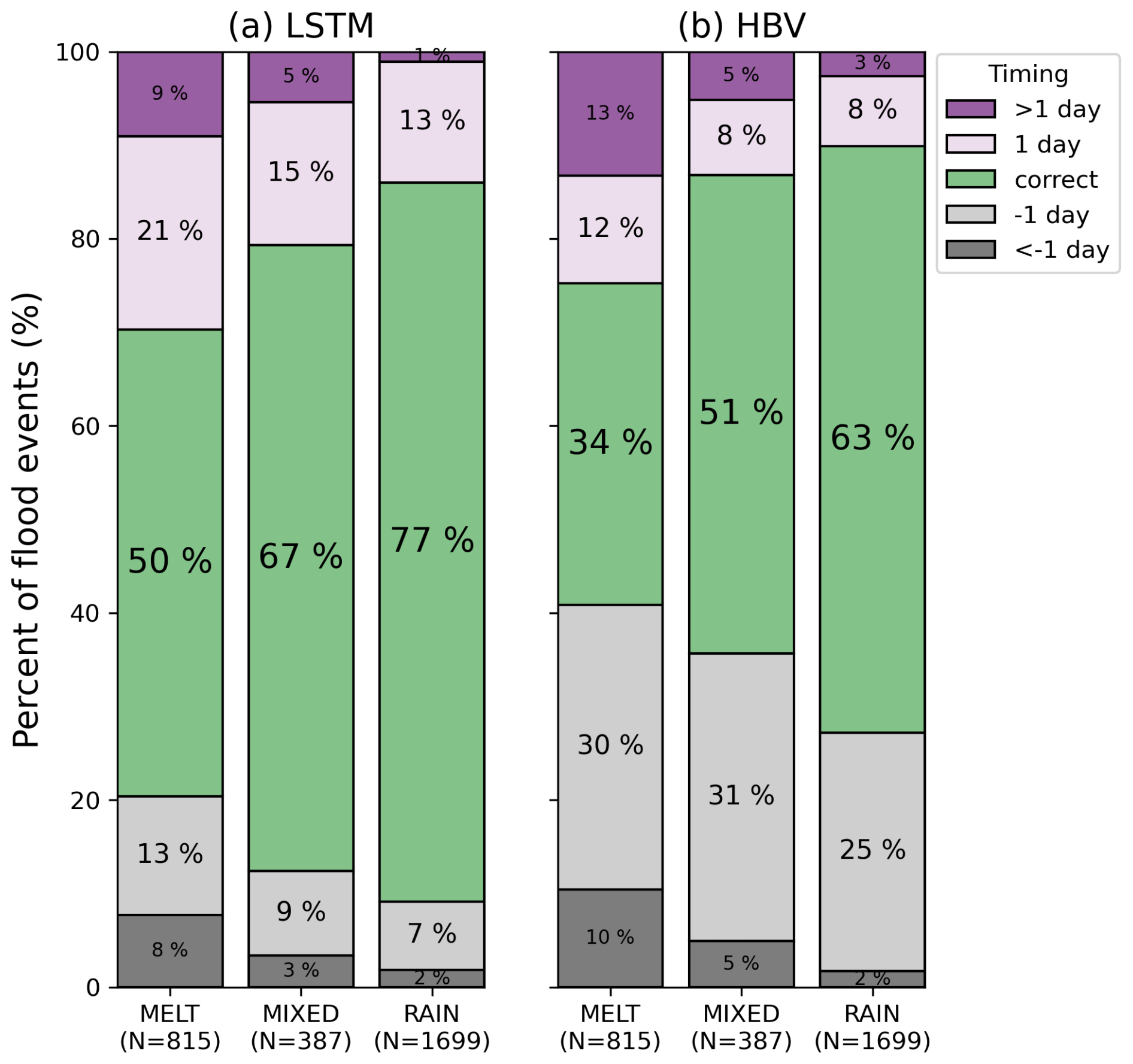
Figure 5 Flood peak timing results for (a) LSTM and (b) HBV of all collected snowmelt generated floods (“MELT”), mixed floods (“MIXED”) and rainfall generated floods (“RAIN”). Shown are the percentages of flood events where the peak day was simulated at the correct day (green), one day too early (light grey), even earlier (dark grey), one day too late (light purple) or even later (dark purple) as compared to observed flood peak day. N values in parenthesis represent the number of flood events.

The distributions of percent error of simulated flood peak magnitudes are relatively similar for snowmelt, mixed and rainfall generated events (Fig. 6). Hence, the two alternative pairs of flood type classification thresholds tested produced very similar results (Figs. C6–C7). Slightly better results were found for PE_{peak,floating} as compared to PE_peak,pinned, as expected since the former allows for extracting the simulated flood peak despite the model missing the peak day by 1 or 2 d (ref. Fig. 5). For LSTM, close to half of the snowmelt (46 %) and rainfall generated events (49 %) are within ±20 % of PE_{peak,floating} values, compared to 36 %, respectively 38 %, of the events for HBV. Regardless of model and flood type, most (77 % to 91 %) of the observed peak magnitudes were underestimated. More events had relatively large underestimations (−40 % to −100 %) for HBV as compared to LSTM.

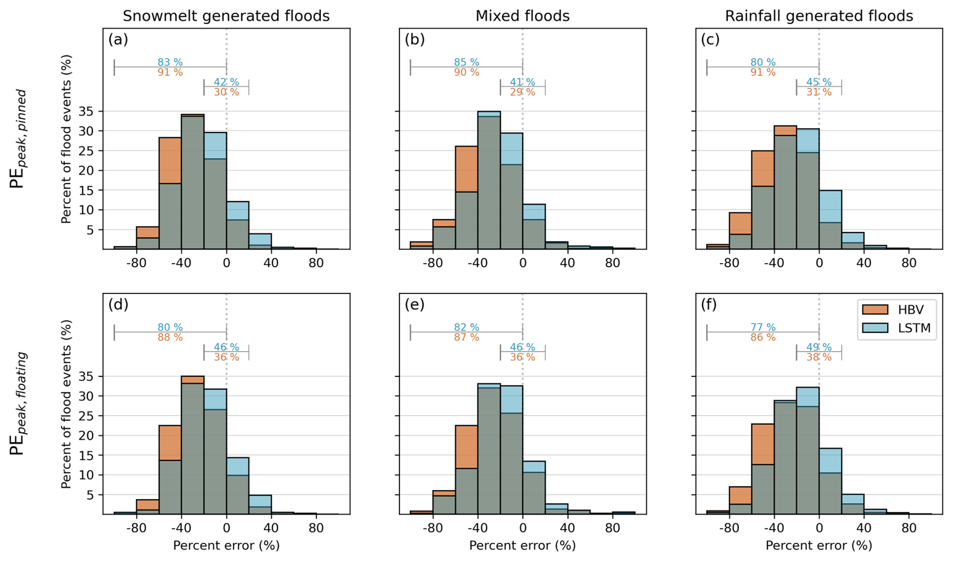
Figure 6 Percent error (PE) of flood peak magnitudes simulated by HBV (orange) and LSTM (blue) for the three different types of flood events: snowmelt generated floods (a, d), mixed floods (b, e) and rainfall generated floods (c, f). Upper panel (a–c) shows the pinned simulations (PE_peak,pinned comparing discharge magnitudes at the day of observed peak), whereas lower panel (d–f) shows the floating simulations (PE_{peak,floating} comparing observed peak discharge with maximum simulated discharge within 2 d of observed peak). In each subplot, the percentage of events that were underestimated (numbers at horizontal line extending −100 % to 0 %), and the percentage of events with a relative error within ±20 % (numbers at horizontal line extending −20 % to 20 %) are shown for LSTM (blue) and HBV (orange).

FAR and POD results for the different flood types and models are shown in Fig. 7. For FAR, a lower value is desirable, whereas a higher value is desirable for POD. As expected, all results allowing for a two day shift in the flood peak timing (“floating”) are better than corresponding results requiring exact day match (“pinned”). Further, using time series specific flood thresholds generally resulted in higher percentages than corresponding results using only observed flood thresholds. LSTM results ranged 21 %–39 % for FAR and 52 %–70 % for POD. LSTM's FAR and POD results for rainfall and snowmelt generated flood events were generally similar, and 6–11 pp better than those of mixed flood events. HBV had slightly higher FAR values (except FAR_floating for mixed and rainfall generated events) and lower POD values than LSTM.

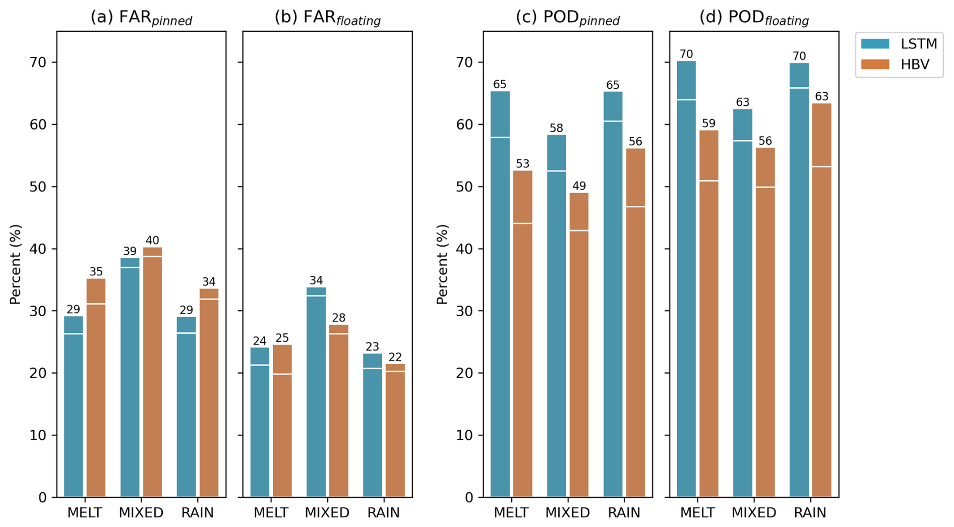
Figure 7 False alarm rate (FAR) and probability of detection (POD) results for LSTM and HBV of all collected snowmelt generated floods (“MELT”), mixed floods (“MIXED”) and rainfall generated floods (“RAIN”). FAR (optimum at 0 %) represents the percent of simulated flood events not exceeding the 98th percentile flood threshold in the observed series (a) at the same day (FAR_pinned) or (b) within 2 d of simulated peak (FAR_floating). POD (optimum at 100 %) represents the percent of observed flood events that also exceed the 98th percentile flood threshold in the simulated series (c) at the same day (POD_pinned) or (d) within 2 d of observed peak (POD_floating). Tallest bars represent results when using the 98th percentile discharge magnitudes defined from each corresponding (simulated or observed) time series, whereas the horizontal white lines represent results when only the observed 98th percentile discharge magnitudes were used.

3.3 Per-catchment flood peak performance

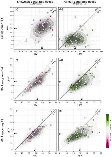
The resulting per-catchment flood peak performance scores for LSTM and HBV are shown in Fig. 8, and maps showing the differences in scores between the two models are presented in Fig. 9. Across all peak metrics and flood types, LSTM had better scores than HBV for the majority of the catchments. LSTM had the lowest percentage of timing error in 84 % of the catchments for snowmelt generated flood events, and 78 % of the catchments in terms of rainfall generated flood events. Median improvement by LSTM across catchments was 14 pp for snowmelt and 11 pp for rainfall generated floods, but improvements exceeding 30 pp were found for several catchments. Both models had a markedly lower timing error when considering rainfall generated events (catchment averages of 24 % for LSTM and 38 % for HBV) as compared to snowmelt generated events (catchment averages of 49 % for LSTM and 66 % for HBV).

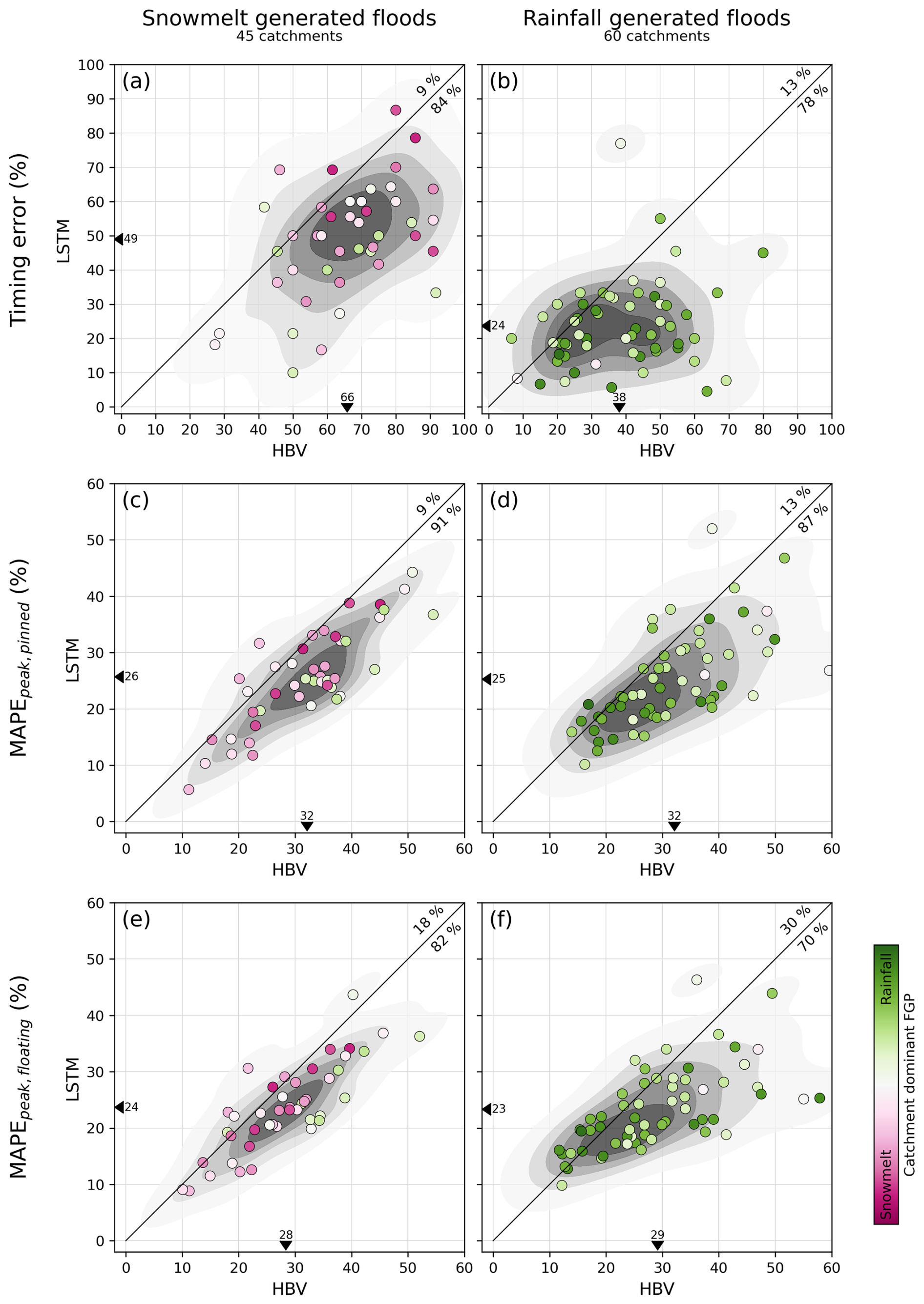
Figure 8 Flood peak performance scores per catchment for HBV (x-axis) versus LSTM (y-axis), for snowmelt generated floods (left) and rainfall generated floods (right). Upper panel (a–b) shows the peak timing error (percentages of incorrectly simulated days of peak discharges). Middle panel (c–d) and lower panel (e–f) show the mean absolute percentage error for pinned simulations (MAPE_peak,pinned comparing discharge magnitudes at the day of observed peak), and for floating simulations (MAPE_{peak,floating} comparing observed peak discharge with maximum simulated discharge within two days of observed peak), respectively. Background is shaded by the corresponding 2D empirical density function. Triangles with adjacent numbers represent catchment average score for each model. Dots below the diagonal line represent catchments with better (i.e. smaller error) metric values for LSTM as compared to HBV. The percentages of catchments above and below the diagonal lines are provided in the upper right corner of each scatterplot. Each catchment is coloured by the corresponding catchment's dominant flood generating process (FGP, ref. Fig. 2).

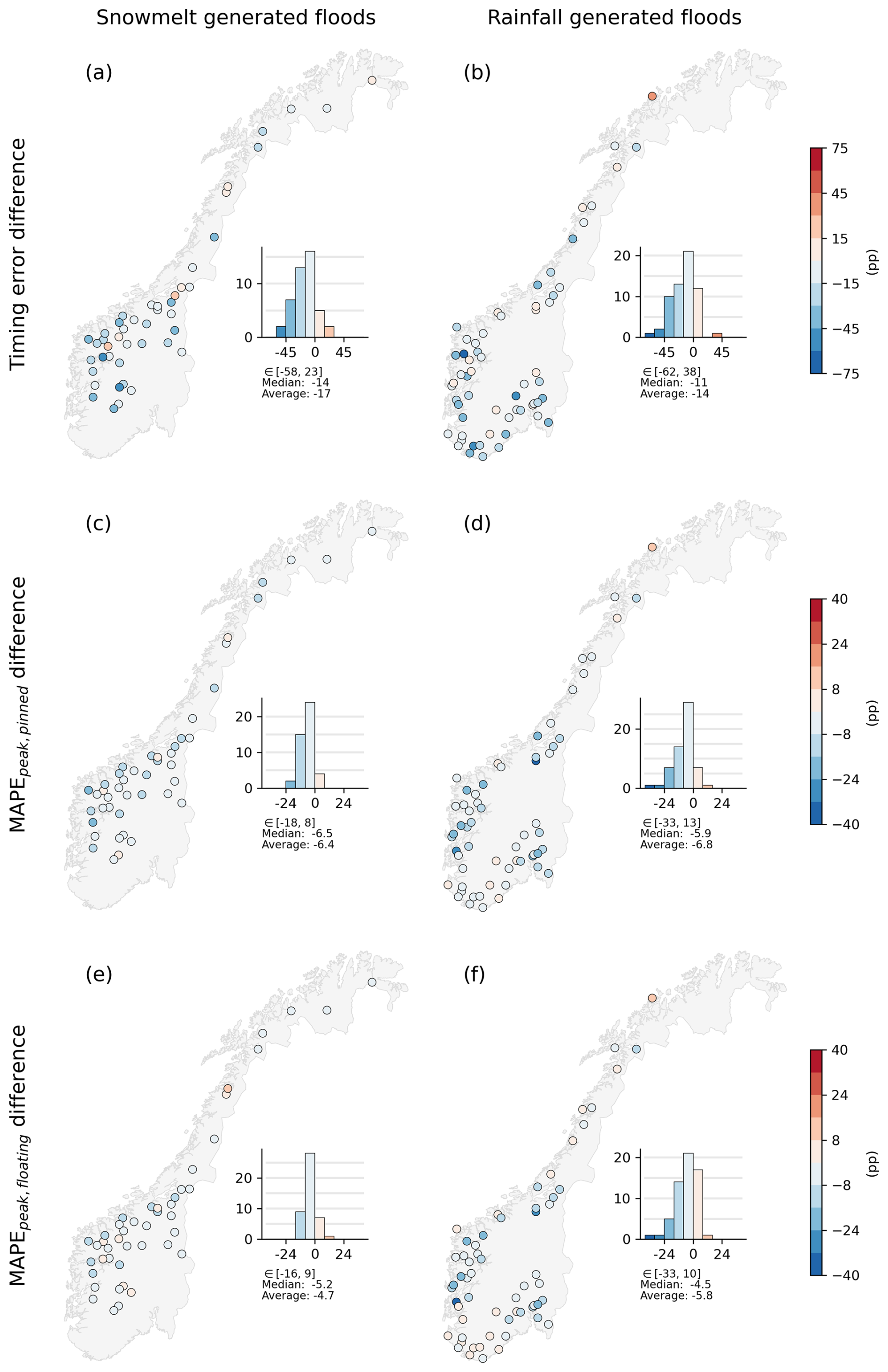
Figure 9 Model difference (LSTM minus HBV results) in per-catchment flood peak performance scores for snowmelt generated floods (left) and rainfall generated floods (right). Upper panel (a–b) shows the model difference in timing error. Middle panel (c–d) and lower panel (e–f) show the model difference in mean absolute percentage error for pinned simulations (MAPE_peak,pinned comparing discharge magnitudes at the day of observed peak), and for floating simulations (MAPE_{peak,floating} comparing observed peak discharge with maximum simulated discharge within two days of observed peak), respectively. Blue colour represents a smaller error for LSTM as compared to HBV. Alongside each map, the corresponding histogram, range, median and average difference are provided.

Most MAPE_peak,pinned scores were in the range 10 % to 40 %, with catchment average of 25 % to 26 % for LSTM and 32 % for HBV. MAPE_peak,pinned for snowmelt generated floods had the largest median model difference of 6.5 pp, in the favour of LSTM. For both error metrics considering peak magnitude (MAPE_peak,pinned and MAPE_{peak,floating}), LSTM had smaller errors than HBV for a larger proportion of the catchments when considering snowmelt generated floods as compared to rainfall generated floods. On the other hand, more catchments had a relatively larger difference between the models when considering rainfall generated floods, in particular for catchments where HBV had a relatively high (>40 %) error score.

Figure 10 combines the model comparisons of overall performance (KGE) and flood peak performance (MAPE_peak,pinned). Catchments in quadrant IV (lower right square in each plot) have a better metric score for LSTM as compared to HBV in terms of both KGE and MAPE_peak,pinned. The majority of catchments (76 % and 75 %) are found in quadrant IV. A few catchments show notably better results for LSTM, with a >0.1 larger KGE and a smaller MAPE_peak,pinned of more than 5 pp. The minority (2 % and 8 %) of the catchments are found in quadrant II that represents better HBV scores for both metrics. Figures C8 and C9 show model difference in NSE, respectively KGE, versus model difference in all three flood peak metrics. In the corresponding plots using NSE instead of KGE, nearly all catchments are located in quadrants I and IV, as LSTM had the highest NSE scores for 96 % of the catchments.

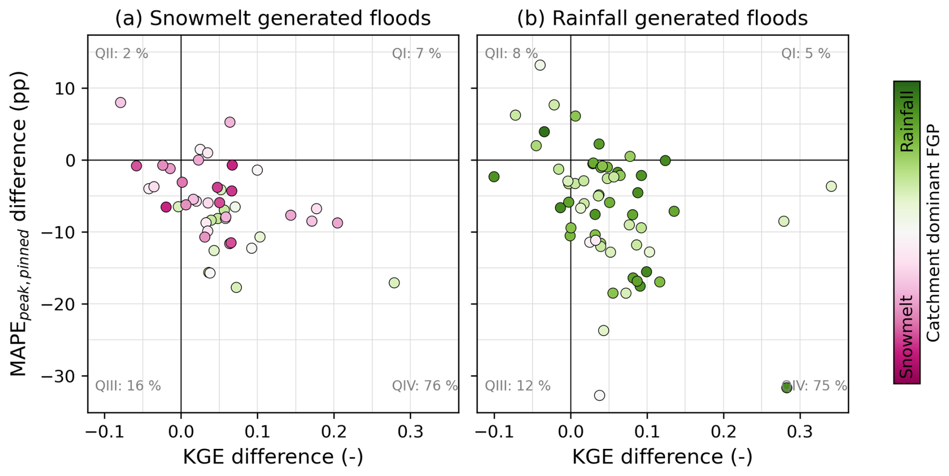
Figure 10 Model difference (i.e. LSTM minus HBV) in the overall performance metric KGE (x-axis) versus the peak metric MAPE_peak,pinned (y-axis) for (a) snowmelt generated floods and (b) rainfall generated floods. Each dot represents a catchment and is coloured by the catchment dominant flood generating process (FGP; ref. Fig. 2). Catchments within quadrant IV (QIV; lower right square) have a better score for LSTM as compared to HBV both in terms of overall performance score and flood peak performance score. Percentages of catchments within each quadrant are given in the corners of the plots.

A per-catchment summary of the best-performing model in terms of all evaluated metrics is presented in Fig. 11. LSTM had the best scores for the majority of the catchments for all evaluated metrics except (the KGE component) γ. For MAE, NSE and ρ, 93 % to 97 % of the catchments had a better score for LSTM. To indicate the catchment specific best model across metrics, the percentage of metrics where LSTM had a better score is given at the top of each catchment column. For eight of the 103 catchments, HBV had better scores for minimum two thirds of the metrics. LSTM on the other hand, had better scores for minimum two thirds of the metrics for 90 of the catchments.

Figure 11 Summary of best performing model in terms of all evaluated metrics and catchments. LSTM has the best score for blue cells, HBV has the best score for light grey cells, and both models have equal scores for dark grey cells. Percentages of blue cells for each catchment (i.e. column) and metric (i.e. row) are provided at the top and right, respectively.

4 Discussion

The LSTM model demonstrated good performance across the metrics assessed in the study. Whereas flood peak timing results were notably better for rainfall as compared to snowmelt generated floods, flood peak magnitudes were simulated with comparable performance for different types of floods. As compared to the benchmark model (HBV), performances were improved for a majority of the catchments in terms of all but one evaluated metrics. The largest improvements by LSTM were often found for metrics and catchments where HBV scores were relatively poor. Thus, the results imply that LSTM can improve hydrological services and flood specific assessments in regions affected by both snowmelt and rainfall generated floods.

4.1 LSTM's ability to simulate different aspects of the streamflow series

LSTM NSE scores were generally high, exceeding 0.7 for 100 catchments, and with an average NSE of 0.84 as compared to 0.76 for HBV. For one catchment in particular (catchment ID 2.439), the models were unable represent the time series well, with NSE<0.6 and KGE<0.7 for both LSTM and HBV. This catchment had calibration NSE of 0.90 (LSTM) and 0.79 (HBV), and a 30 % drop in runoff coefficient from training to evaluation period, indicating problems with the observed meteorological or streamflow data during the evaluation period rather than an inability of the models to represent the catchment's streamflow behaviour. Many of the snowmelt dominated catchments were among the catchments with the highest NSE scores for HBV, in line with previous studies demonstrating that models typically achieve higher NSE and KGE values in catchments with strong seasonality (Ruzzante et al., 2026; Anderson and Radić, 2022). However, for LSTM in terms of NSE, and for both models in terms of KGE, there were no distinct relation between catchment dominant FGP and model performance score.

A higher percentage of catchments were improved by LSTM in terms of NSE (96 %) as compared to KGE (77 %). Of the three components constituting KGE, the one reflecting the variability (γ) of the model was the only evaluated metric with a better HBV score for the majority of the catchments (Fig. 11). LSTM generally underestimated γ for more catchments and to a larger degree than HBV (Fig. C2). The underestimated variability may partly relate to the applied loss function (NSE) which normalises the prediction errors by the variability of the time series. Gupta et al. (2009) has previously shown how the variability has to be underestimated to maximise NSE. In terms of the bias ratio (β), the majority of catchments exhibited better scores for LSTM than HBV. Due to precipitation undercatch, the HBV model includes catchment specific correction factors for rain and snow precipitation that were calibrated to support conservation of the water balance. The LSTM model, on the other hand, has no water balance constraints and has therefore no need for precipitation correction factors. We suggest that the improved bias ratios obtained by LSTM result from the absence of water balance constraints, allowing for a more accurate representation of average streamflow. Further, LSTM outperformed HBV in all but three catchments in terms of mean absolute error, implying a systematically higher accuracy in the LSTM predictions.

4.2 Within-model differences in flood peak performance for snowmelt versus rainfall generated floods

The results revealed notable differences in the ability of LSTM to simulate the correct peak timing of snowmelt versus rainfall generated floods. Whereas 77 % of rainfall generated flood peaks were simulated at the correct day, the corresponding percentage for snowmelt generated flood peaks was only 50 % (Fig. 5). This finding was robust across the three different pairs of classification thresholds tested (Figs. C3–C5). As snowmelt generated floods react to snowmelt typically spanning days to weeks, the floods often last multiple days and may not have a very distinct peak as compared to rainfall generated floods (e.g. Fig. 2 in Barna et al., 2023b). Relatively small differences between peak discharge and discharge magnitudes in adjacent days may explain the lower percentage of correctly simulated peak days for snowmelt generated floods. This reasoning is supported by the similar mean absolute percentage errors at the day of observed peak (MAPE_peak,pinned) and FAR and POD results for snowmelt and rainfall generated floods (Fig. 8). The same reasoning may explain the intermediate position of the timing results for mixed flood (better than snowmelt generated floods and worse than rainfall generated floods).

The identified differences in model performance for different flood types were not unique to LSTM. Similar differences were found for HBV. In terms of MAPE_peak,pinned, HBV exhibited the highest errors (exceeding 40 %) for rainfall generated floods in several catchments. Similarly high errors were only found in three catchments for LSTM. Flood-type dependent performance has also previously been demonstrated by Brunner et al. (2021), who identified differences in a model's flood peak performances in catchments of different regimes across four different process-based hydrological models.

4.3 Model evaluations reflecting the characteristics of interest

The value of a hydrological model for specific applications depends on the model performance with regards to relevant characteristics. Thus, model evaluations beyond the metrics considering the entire streamflow time series (e.g. NSE and KGE) are often necessary. Figure 10 shows that the model preferred for simulating the full streamflow time series (KGE) does not always match the one preferred for reproducing peak magnitudes (MAPE_peak,pinned). Whereas the majority of the catchments had better LSTM scores for both overall and flood peak metrics (quadrant IV), the preferred model depended on the metric for approx. one fifth of the catchments (quadrants I and III). Notably, some catchments had a slightly (<0.025) lower KGE for LSTM than HBV, whereas the peak magnitude errors were reduced by 5 to 10 pp. In such cases, LSTM may be the preferred model for flood-specific applications despite the somewhat lower overall score.

We included three different flood peak specific evaluation metrics in this study to account for different aspects relevant for flood applications. Specifically, MAPE_peak was evaluated both for simulated discharge at the day of observed peak (“pinned”), and for simulated maximum discharge within 2 d of the observed peak (“floating”). For HBV, which generally had higher timing errors, the differences between the two MAPE_peak metrics were larger than for LSTM. However, the overweight of catchments with a better LSTM MAPE_{peak,floating} score make evident that peak magnitudes were better represented by LSTM regardless of the timing errors by HBV. Generally, our flood peak evaluation results demonstrated that LSTM does a better job than HBV for most catchments. At the local (i.e. catchment) scale, however, the conclusion on the preferred model depends in some cases on the desired characteristic, and the desired characteristics depend on the application. For issuing flood warning, for example, the timing may be crucial, whereas inundation mapping depend more on magnitudes being correctly simulated.

A related interesting model evaluation step, outside of scope of this study, is to evaluate to what degree flood event classification using data from the hydrological models correspond to the applied classification. However, such an evaluation has to be done differently for the two models. For HBV, flood classification using model simulated snowmelt and derived rainfall can be compared with the classification performed using SeNorge derived rainfall and snowmelt. LSTM, on the other hand, does not simulate snowmelt, and an evaluation of its ability to classify flood events into dominant FGP, would rely on explainable machine learning techniques. One such technique proposed by Jiang et al. (2022) uses integrated gradients to trace back contributions of each input sequence (precipitation and temperature) to individual flood events, and applies cluster analysis to identify dominant flooding mechanisms. They identified three main FGPs across Europe, two of them dominating in Norway and strongly reflecting snowmelt and rainfall generated flood events, respectively. A primary aim of a comparison of such a classification approach with the one used here, could be to assess the robustness of classification technique and subjective choices regarding FGP definitions. The relatively simple classification technique and related subjective choices used in this study is subject to uncertainties, and a comparison with other techniques would be an interesting further study. That said, we expect limited effect of chosen technique on our main results and conclusions, as indicated by the very similar results produced using alternative classification thresholds.

4.4 Training LSTM on the premises of deep learning models

In this study, we constrained the dynamical forcing data and training period for LSTM to match that of our benchmark model in order to have a reasonably fair comparison. By doing so, we ensured that differences in model performances could not be attributed to differences in how informed the models were about local hydrometeorological conditions in each catchment. However, given the fundamentally different nature of the two models, the premises for training the best model are different. Accordingly, premade choices suitable of the benchmark model is not the best suitable choices for deep learning models, and there is a further potential to improve the LSTM simulations. Low-hanging fruit to achieve an LSTM model with even higher performance include expanding the training period considerably where possible and forcing the model with a wider range of atmospheric variables and datasets (Martel et al., 2025; Kratzert et al., 2021). Another possibility is finetuning of the LSTM model for individual catchments to explore the potential to improve the model further for local conditions (Kratzert et al., 2018). Such potential avenues should be explored in case an LSTM model is considered for operational use to unleash the best potential based on the premises of deep learning models.

5 Conclusions

This study evaluated the ability of LSTM to simulate floods of different flood generating processes by assessing peak timing and peak magnitude of snowmelt generated floods and rainfall generated floods separately. To evaluate LSTM's potential for operational use in snow-influenced regions, the results were compared with the operational model in the study region, HBV. Our findings can be summarised by the following answers to our research questions:

1. LSTM simulated streamflow series with higher performance than HBV for 96 % of the catchments in terms of NSE and 77 % of the catchments in terms of KGE. The largest improvements by LSTM were found for catchments with the lowest HBV performance scores.

2. LSTM simulated the correct timing of the flood peaks more often for rainfall generated events (77 %) than mixed events (67 %) and snowmelt generated events (50 %). The percentages of correctly simulated peak timing were 14–16 pp higher than those of HBV for all snowmelt, mixed and rainfall generated events, mainly because HBV more frequently simulated peak discharge too early.

   LSTM simulated flood peak magnitudes with a similar performance for snowmelt generated floods, mixed floods and rainfall generated floods. Percent errors were within ±20 % for close to half of the events, a slightly better result than that of HBV. Both LSTM and HBV generally underestimated flood peak magnitudes, whereas HBV had a higher proportion of the largest underestimations (more than 40 % underestimation) as compared to LSTM for the three types of floods. Resulting false alarm rates and probabilities of detection were similar for rainfall and snowmelt generated events, and slightly better than those of mixed flood events.

3. A large spread among catchments was found in timing errors by LSTM for snowmelt generated floods (approx. 10 % to 80 %), with an average of 49 %. Timing errors for rainfall generated floods were notably smaller, with an average error of 24 % and only two catchments exceeding 50 %. LSTM exhibited smaller timing errors than HBV in the majority of the catchments for both snowmelt and rainfall generated floods.

   Per-catchment LSTM results of mean absolute percentage error of flood peaks were mainly in the range 10 % to 40 % for both snowmelt and rainfall generated flood events. For both types of floods, the errors were smaller for LSTM as compared to HBV for the majority of the catchments. Most model differences were within 16 pp, but LSTM improved the rainfall generated flood peak magnitude simulations with up to 33 pp for catchments with relatively poor HBV scores.

Overall, LSTM provided reliable simulations of streamflow time series and floods of different flood generating processes in catchments influenced by seasonal snow. Notable improvements were found in the timing of simulated flood peaks, and in overall and peak magnitude metrics for catchments where the benchmark model had relatively poor results. Our findings highlight LSTM's potential to improve hydrological services and flood assessments in regions prone to both snowmelt and rainfall generated floods.

Appendix A: Training the LSTM model

The LSTM model was trained using the 15-years period 1 September 2009–31 August 2024, to match the calibration period used for our benchmark model simulations. The catchment-averaged NSE, used as loss function, was minimised using the Adam optimiser (Kingma and Ba, 2017) and we used a linear output activation function. The forget gate bias was initialised to 3, a common practice that encourages the LSTM to retain information early in training (Frame et al., 2022; Gauch et al., 2021). To stabilise training, gradient norms were clipped to a maximum value of 1. The model was validated at every epoch, evaluating performance on 50 randomly selected catchments from the validation set. To mitigate overfitting during training, the final hidden state vector h_t was passed through a dropout layer, which randomly sets each element to zero with probability p_dropout.

The hidden state dimension, dropout probability, batch size (the number of training examples used to compute the loss gradient in each model update), input sequence length and learning rate were treated as tunable hyperparameters. These hyperparameters were tuned in a 5-fold cross-validation (CV) over the period 1 September 2009–31 August 2024. For each of the five CV-iterations, the period was split into a validation period of three consecutive years, and a left-out-fold of three consecutive years. Each year was used as left-out-fold once and validation period once during the CV. The years adjacent to the left-out-fold were removed to have a temporal “buffer” between the left-out-fold and the “seen” years, and the remaining years comprised the training period in each CV-iteration. The following hyperparameter values were considered in a grid search in each CV split (selected values for final model in bold):

• Hidden state dimension = [64, 128, 256]

• Dropout probability = [0.2, 0.3, 0.4]

• Batch size = [64, 128, 256]

• Input sequence length = [270, 365]

• Learning rate = [0: 1e-3 10: 5e-4 25: 1e-4, 0: 5e-3 10: 1e-3 25: 5e-4]

where the learning rate schedule notation indicates the learning rate value at specified epochs (i.e. epochs 0, 10, and 25). This yielded 108 hyperparameter combinations per cross-validation split. The number of training epochs (from 1 to 50) was selected by evaluating validation NSE at each epoch for each hyperparameter combination.

Models using the faster learning rate schedule frequently exhibited poor performance (low or negative validation NSE) and training instability, leading us to exclude these configurations from further consideration. For the remaining 54 hyperparameter combinations per split, we evaluated performance on the left-out-fold using the three epochs with highest catchment-averaged validation NSE: epoch 35 (NSE = 0.852), epoch 26 (NSE = 0.850), and epoch 10 (NSE = 0.849).

The final hyperparameter configuration (shown in bold above) was selected as the combination yielding the highest average NSE across all left-out-folds and evaluated epochs. The final model was trained using 1 September 2009–31 August 2019 as the training period and 1 September 2019–31 August 2024 as the validation period. We selected epoch 35 for the final model as it achieved the highest catchment-averaged validation NSE of 0.87.

Appendix B: HBV calibration

For descriptions of the version and set-up of the daily HBV model used operationally in Norway, we refer to Lawrence et al. (2009) and Ruan and Langsholt (2017), except that the model has been re-calibrated for a more recent period (1 September 2009–31 August 2024) using a more recent meteorological dataset (SeNorge_2018) after the two reports were published. In short, the applied HBV model is a semi-distributed bucket-type model, that divides the catchment into ten elevation zones to account for elevation gradients in temperature and precipitation (Sælthun, 1996; Killingtveit and Saelthun, 1995). The model uses elevation zone averaged daily precipitation sums and mean temperatures as input. Fluxes between and processes within four storage components, i.e. snow, soil moisture, an upper runoff zone, and a lower runoff zone, are represented by simplified process-based expressions.

We calibrated the HBV model using the operational model's calibration set-up and choices, except that we used Nash-Sutcliffe efficiency (NSE) as a loss function to match that of LSTM. Catchment-by-catchment calibration was conducted using Model-Independent Parameter Estimation and Uncertainty Analysis (PEST; Doherty, 2004) with parameter ranges from Table 1 in Ruan and Langsholt (2017). Daily discharge and meteorological observations in Norway have historically been recorded at two different daily divides, i.e. 00:00–00:00 CET and 07:00-07:00 CET, respectively. In the HBV model used operationally, discharge and meteorological data are matched using the largest overlap possible (17 h). Correspondingly, we kept this choice for the modelling of both HBV and LSTM.

Appendix C: Additional figures

Figure C1 Runoff coefficient (i.e. ratio of streamflow (mm d⁻¹) to precipitation (mm d⁻¹)) of each catchment in the training period (i.e. calibration period; x-axis) versus the evaluation period (y-axis). A dot close to the diagonal line implies consistent runoff coefficients for the two periods. Catchments with glaciers covering more than 3 % of their area are marked with stars. We note that values exceeding 1 (i.e. streamflow larger than precipitation) are mainly due to underestimation of precipitation, although glacier melt can explain part of the difference in catchments with glaciers. Each catchment is coloured by the corresponding catchment's dominant flood generating process (FGP, ref. Fig. 2).

Figure C2 Overall performance per catchment for HBV (x-axis) versus LSTM (y-axis) in terms of the three KGE components (a) correlation coefficient, ρ, (b) bias ratio, β, and (c) variability ratio, γ, as well as (d) mean absolute error, MAE. Optimum values are marked with stippled lines. Backgrounds are shaded by the corresponding 2D empirical density functions. Triangles with adjacent numbers represent catchment average score for each model. The percentages of catchments above and below the diagonal lines are provided in the upper right corner of the scatterplots of ρ and MAE. For β and γ, percentages of scores below and above optimum value of 1 are provided for both models. Each catchment is coloured by the corresponding catchment's dominant flood generating process (FGP, ref. Fig. 2).

Figure C3 Distribution of all flood events' fractional rainfall contribution. Dark green vertical lines represent flood type classification thresholds used for the main analyses. Light green and blue vertical lines represent two alternative pairs of classification thresholds for which Figs. 5 (flood peak timing) and 6 (flood peak magnitude) have been repeated (see Figs. C4–C7).

Figure C4 As Fig. 5, but using the alternative symmetric thresholds 0.2 and 0.8 for flood type classification (see Fig. C3). Note that the values in parenthesis, representing the number of flood events, are different from Fig. 5.

Figure C5 As Fig. 5, but using the alternative asymmetric thresholds 0.3 and 0.9 for flood type classification (see Fig. C3). Note that the values in parenthesis, representing the number of flood events, are different from Fig. 5.

Figure C6 As Fig. 6, but using the alternative symmetric thresholds 0.2 and 0.8 for flood type classification (see Fig. C3).

Figure C7 As Fig. 6, but using the alternative asymmetric thresholds 0.3 and 0.9 for flood type classification (see Fig. C3).

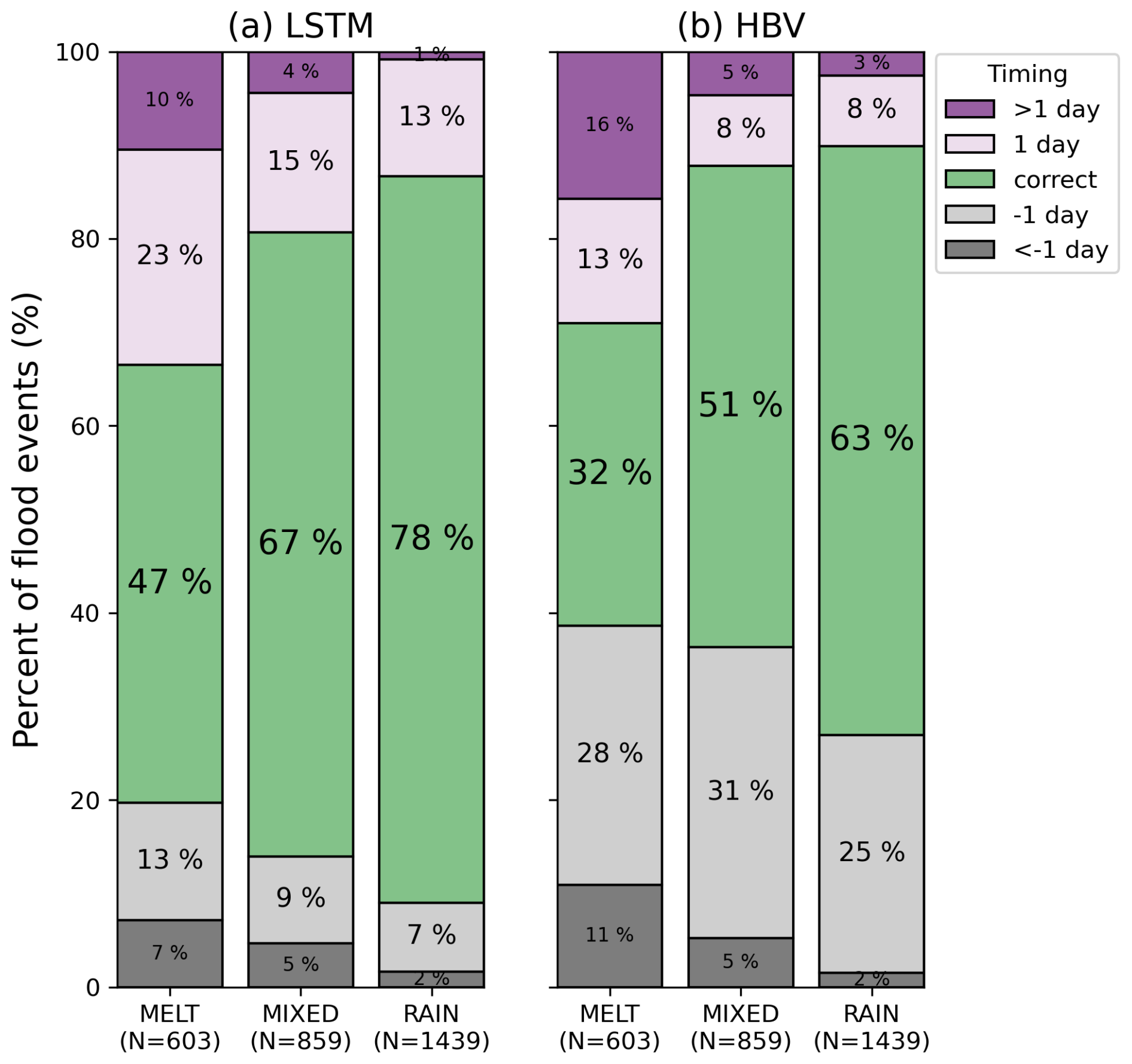
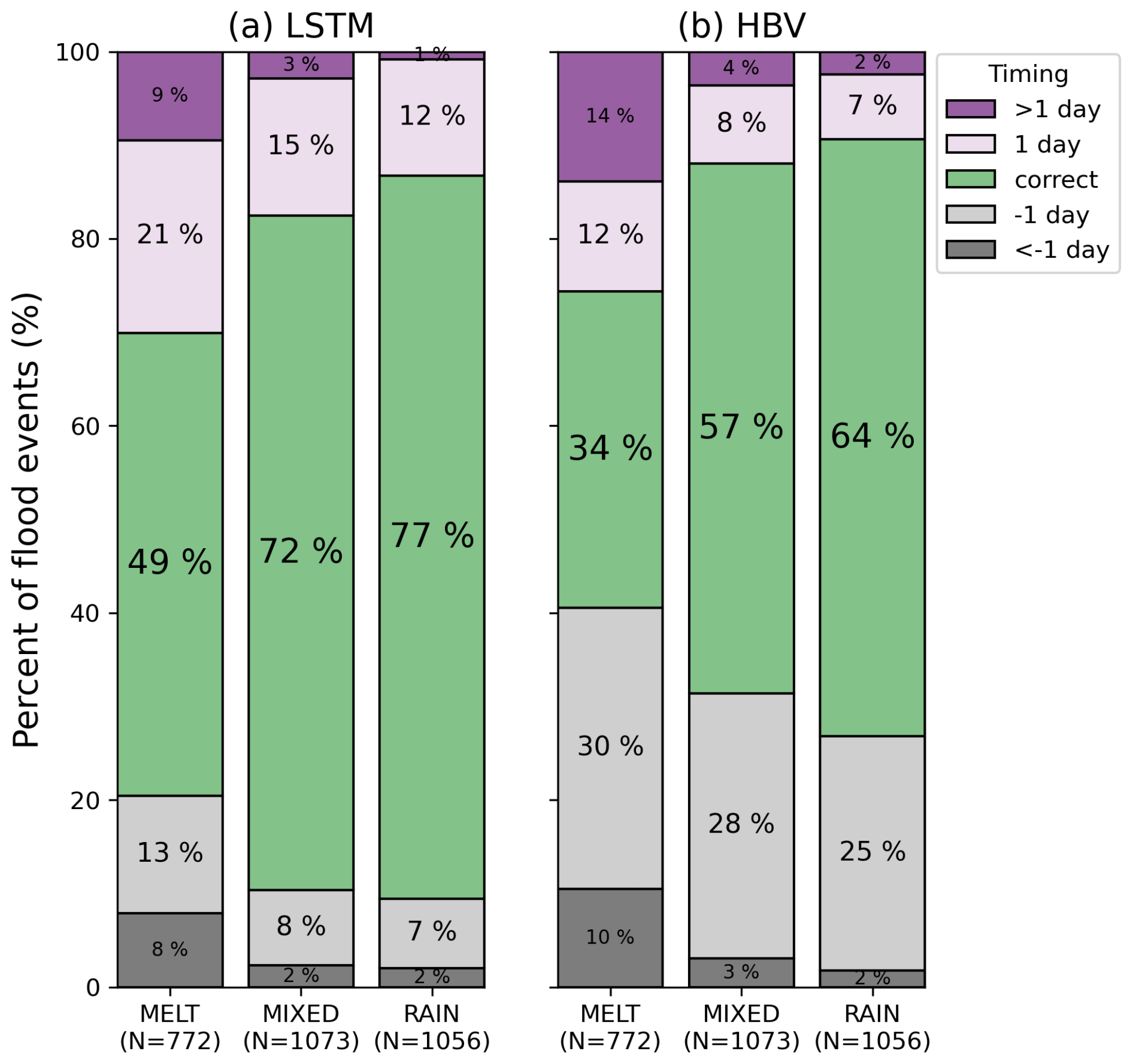
Figure C8 Model difference (i.e. LSTM minus HBV) in the overall performance metric NSE (x-axis) versus the flood peak metrics: (a–b) timing error, (c–d) MAPE_peak,pinned and (e–f) MAPE_{peak,floating}, separately for snowmelt generated floods (left) and rainfall generated floods (right). Each dot represents a catchment and is coloured by the catchment's dominant flood generating process (FGP; ref. Fig. 2). Catchments within quadrant IV (QIV; lower right square) have a better score for LSTM as compared to HBV both in terms of overall performance score (NSE) and flood peak performance score. Percentages of catchments within each quadrant are given in the corners of the plots.

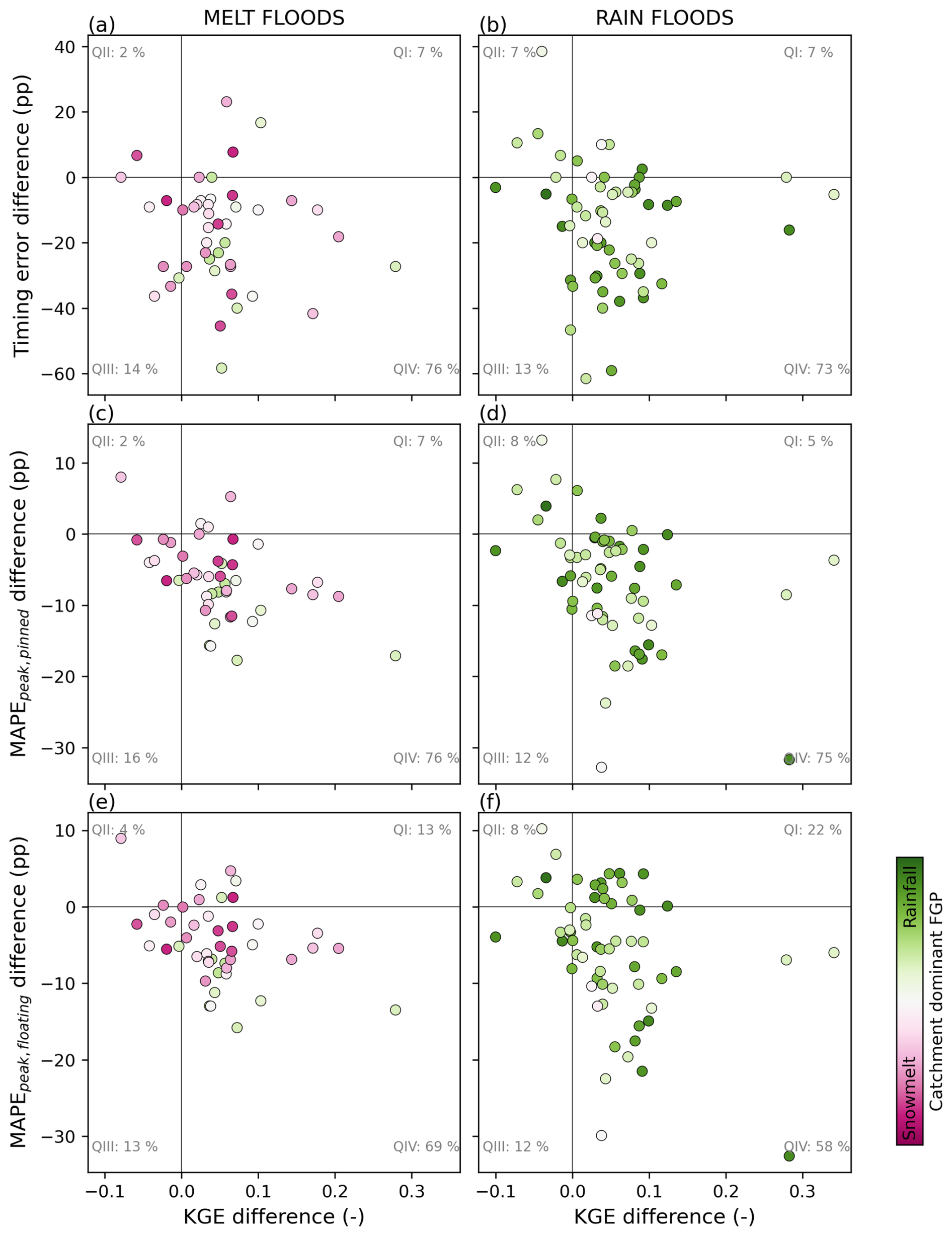
Figure C9 Model difference (i.e. LSTM minus HBV) in the overall performance metric KGE (x-axis) versus the flood peak metrics: (a–b) timing error, (c–d) MAPE_peak,pinned and (e–f) MAPE_{peak,floating}, separately for snowmelt generated floods (left) and rainfall generated floods (right). Each dot represents a catchment and is coloured by the catchment's dominant flood generating process (FGP; ref. Fig. 2). Catchments within quadrant IV (QIV; lower right square) have a better score for LSTM as compared to HBV both in terms of overall performance score (KGE) and flood peak performance score. Percentages of catchments within each quadrant are given in the corners of the plots.