Climatology and trends of extreme precipitation in France: evaluation of an explicit-convection regional climate model

Climate change is intensifying the global water cycle, with extreme precipitation events increasing in frequency and intensity at the global scale. While trends in daily precipitation extremes are well-documented, sub-daily extremes – critical for flash flood risk – remain poorly characterized, due to limited long-term sub-daily observations. Convection-permitting models explicitly resolve deep convection and therefore offer the potential for a substantially improved representation of convective processes and short-duration precipitation extremes. This study evaluates the ability of the convection-permitting regional climate model AROME (2.5 km resolution, 1959–2022), forced by ERA5 reanalysis, to reproduce precipitation extremes and their trends, at daily and hourly scales, using a dense network of Météo-France stations.

Using extreme value theory (GEV modeling), we analyze trends in 10-year return levels for both daily (1959–2022) and hourly (1990–2022) extremes. At the daily scale, AROME reproduces observed positive trends in southeastern France, consistent with previous studies. Hourly trends are more heterogeneous and less robust, with high spatial variability and low model-observation correlation. Overall, the results demonstrate the value of the explicit-convection model for studying extreme precipitation, while also highlighting its limitations for convective extremes.

1 Introduction and context

Climate change is driving a warming of the planet's surface air, with a more pronounced increase over land than over oceans (IPCC, 2021). Global warming has reached +1.1 °C worldwide, +1.7 °C in metropolitan France, and +2 °C in the French Alps compared to the pre-industrial era. Furthermore, the Clausius–Clapeyron relationship indicates that warmer air can hold more moisture (+7% °C⁻¹) (Clapeyron, 1834). Surface warming leads to atmospheric warming, which increases the water-holding capacity of the troposphere according to the Clausius–Clapeyron relationship (Clapeyron, 1834; Trenberth et al., 2003; Westra et al., 2013), while the actual condensation and precipitation are driven by vertical motion and adiabatic cooling of ascending air masses (O'Gorman and Muller, 2010). However, for non-extreme or average precipitation events, the central portion of the precipitation distribution does not fully capitalize on this excess moisture. Energetic constraints (radiative balance, evaporation, ocean-air exchanges) and dynamic constraints (subsidence, synoptic winds) limit the increase in mean precipitation to only 1 % °C⁻¹–3% °C⁻¹ (IPCC, 2021). In contrast, during intense convective events (thunderstorms, rapid cyclogenesis), rapid ascent condenses nearly all of this surplus, causing short-duration extreme rainfall to increase by 5 % °C⁻¹–8 % °C⁻¹ – almost matching the theoretical potential. Extreme precipitation closely follows the Clausius–Clapeyron scaling, whereas mean rainfall remains influenced by numerous other energetic and dynamic factors (O'Gorman, 2015). Thus, climate warming theoretically leads to an increase in extreme precipitation, though this increase varies with changes in atmospheric circulation and can be locally amplified (Blanchet et al., 2021).

Extreme precipitation events are defined as events belonging to the upper tail of the precipitation intensity distribution. There is no consensus on what constitutes an extreme event. Some authors study precipitation intensities above the 99th percentile or seasonal/annual maxima, while others define extreme precipitation as events rarely or never encountered in a human lifetime (e.g., precipitation levels expected once every 50, 100 or 1000 years). Extreme events are at the heart of climate and societal concerns, as they are responsible for numerous casualties and economic costs associated with flooding, landslides, and infrastructure failures (IPCC, 2022). In 2024, numerous such events made headlines, including in Nepal, Afghanistan, Central Europe, eastern Spain, and France (World Meteorological Organization (WMO), 2025). Notably, in France in June 2024, intense high-altitude rainfall contributed to major flooding in the Écrins massif (Blanc et al., 2024); in October 2024, over 600 mm of rain in 48 h caused widespread flooding in the western slopes of the Massif Central (Météo-France, 2024a); and in May 2025, extremely intense but short-lived thunderstorms (locally exceeding 120 mm h⁻¹) caused extensive damage in the central Mediterranean region (Météo-France, 2025a).

Daily extremes have increased in intensity and frequency across more than half of the world's land regions, at a rate close to +7% °C⁻¹ of warming (IPCC, 2021). Some regional studies suggest similar trends in a significant proportion of land areas (Donat et al., 2016). In France, however, signals are far more heterogeneous, with strong regional variations. In most regions, trends remain weak or non-significant, and only in certain areas – particularly the southeast – are signals detected. In southeastern France, no significant trend in annual maxima of daily precipitation was detected before the early 1990s (Blanchet and Creutin, 2022). Since then, studies report increases on the order of 20 % (with estimates reaching up to +40 % depending on the metric and uncertainty range) (Ribes et al., 2019; Blanchet et al., 2018; Blanchet and Creutin, 2022). In the southeastern Alps, the increase in 20-year return level daily precipitation in autumn reaches up to +100 % between 1958 and 2017 (Blanchet et al., 2021).

Hourly extremes are essential for characterizing intense convective phenomena (thunderstorm downpours, stationary thunderstorms) often responsible for flash floods. Due to the lack of long, spatially dense time series, there is no systematic global analysis of sub-daily trends; available data are often sparse, short, and non-significant. Nevertheless, several regional studies detect an intensification of hourly extremes across nearly all continents, though global confidence in an overall increase remains very low (IPCC, 2021). Increases in extreme rainfall have been observed in the United States, China (summer), Australia (annually), South Africa (summer), India, Malaysia, and Italy (IPCC, 2021). Depending on the method and region, studies highlight temperature-scaling rates ranging from +7 % °C⁻¹ to +13% °C⁻¹ – up to twice the Clausius–Clapeyron rate (Molnar et al., 2015). In France, few regional studies explicitly characterize trends in hourly return levels and percentiles. Observed maximum 1 h values now reach 40–60 mm during major Mediterranean events, compared to 30–40 mm in the 1980s–1990s (Météo-France, 2024b). Only the study by Berghald et al. (2025a) quantifies trends in hourly extremes in the French Alps. However, trends in hourly return levels remain weak to non-significant, with no clear spatial or seasonal coherence, contrasting with the robust signals observed at daily time scales (Soubeyroux et al., 2015). This suggests that hourly extremes do not yet show a clear climate signal, possibly because the signal is still emerging but cannot be robustly detected given the short length of available series and the high year-to-year variability.

In France, a nationwide network of daily precipitation with good spatial coverage became available from the 1950–1960s, while most hourly records only began in the 1990–2000s (Météo-France, 2024b). In parallel, regional climate models (RCMs, about 12 km resolution for EURO-CORDEX) forced by reanalyses provide complementary advantages of: (1) precipitation series that potentially go back further in time than raingauge records; and (2) spatially complete and physically consistent fields, particularly useful in poorly instrumented areas. Although RCMs are useful for studying daily extremes (Dierickx et al., 2025; Steensen et al., 2025), they are not suitable for studying convective extremes, as convection is parameterized, leading to over-smoothed and poorly located hourly precipitation at 12 km resolution (Schär et al., 2020). The emergence of RCMs at kilometer-scale resolution allowing the explicit resolution of deep convection offers a unique opportunity, as they realistically simulate the dynamics of intense precipitation at fine spatial and temporal scales. However, conducting multi-decadal hindcasts is computationally challenging for CPMs, which makes our 63-year simulation particularly valuable. Recent multi-model convection-permitting ensembles have been shown to better represent heavy precipitation compared to 12 km resolution RCMs, in particular at hourly scale (Ban et al., 2021; Pichelli et al., 2021; Berthou et al., 2020). Such simulations also provide more certain projections of local changes in extreme rainfall, by substantially reducing model-related uncertainty compared to coarser-resolution RCMs (Fosser et al., 2024). The convection-permitting RCM model developed by CNRM (CNRM-AROME model, 2.5 km) forced by the global reanalysis ERA-Interim (80 km) has been evaluated by Caillaud et al. (2021) over the Pan-Alpine domain (1981–2018) and by Cortés-Hernández et al. (2024) over Corsica island (2000–2018). Caillaud et al. (2021) show a generally good representation of heavy precipitation events, but the model tends to underestimate the highest values (> 200 mm d⁻¹ and > 40 mm h⁻¹).

Recently, a new hindcast simulation using the latest version of the CNRM-AROME model and forced by the ERA5 reanalysis at 50 km (native ERA5 resolution ∼ 30 km) has been performed, covering the period from 1959 to 2022. This provides a unique dataset with sufficiently long series (63 years) to study precipitation extremes in France and their trends. However, the validity of the extremes simulated by this model has never been evaluated. Our study aims at addressing this gap. In addition to evaluating new simulations, our study shows two added-values compared to Caillaud et al. (2021), Ban et al. (2021) or Pichelli et al. (2021). First, we focus here on extremes, i.e. precipitation amounts observed only a few times in a lifetime (e.g. the 10-year return level, which is the level exceeded on average once every ten years), rather than heavy precipitation corresponding to high but non-extreme quantiles (e.g. the 99th percentile of daily precipitation considered in Ban et al. (2021) is exceeded on average 3.65 times a year, while the 99.9th percentile of hourly precipitation is exceeded on average once in 40 d). Second, we evaluate trends in extreme precipitation, whereas Caillaud et al. (2021), Ban et al. (2021) or Pichelli et al. (2021) looked at the climatology. Based on non-stationary Extreme Value Theory, our analysis is able to evaluate trends in 10-year return level in CNRM-AROME at both daily and hourly scale in France.

2 Data used

2.1 Stations

In order to evaluate the CNRM-AROME model, this study uses precipitation data from Météo-France stations (Météo-France, 2024b) at daily (1959–2022) and hourly (1990–2022) time steps. There is a strong contrast between daily and hourly observational records available in France. Daily stations provide long, dense time series: more than half of the 8198 daily records have over 40 years of data with limited missing values, and several exceed 60 years. In contrast, hourly stations remain much shorter: most of the 2315 hourly stations offer only 15–30 years of data, reflecting the later deployment of automatic networks. This disparity underscores why long-term trends in sub-daily extremes have been little studied in France so far.

Station selection is based on two criteria: at each station, we compute the proportion of missing data for each year/season/month. A year/season/month is considered as missing if it contains more than 10 % of missing values. Then only the stations with at least the required number of nonmissing years/seasons/months are retained: 50 years for the daily station (1959–2022) and 25 years for the hourly stations (1990–2022). Subsequent analyses are restricted to this subset of stations and years/seasons/months. These criteria, applied over the complete hydrological reference period, lead us to select 1583 daily stations and 574 hourly stations.

2.2 CNRM-AROME model

CNRM-AROME model (hereafter referred to as AROME) is the Convection-Permitting Regional Climate Model (CP-RCM) developped at CNRM (Centre National de Recherches Météorologiques). Based on the limited-area mesoscale AROME model (Seity et al., 2011) used for National Weather Prediction at Météo-France since 2008, AROME is also used in climate mode since 2014 (Caillaud et al., 2021; Lucas-Picher et al., 2024a). AROME combines the non-hydrostatic dynamical ALADIN bi-spectral core and physical parameterisations coming from the research model Meso-NH. At the kilometer-scale resolution, deep convection is no longer a sub-grid process but shallow convection still need to be parametrised. A new version of AROME is used in this study, with improvements mainly concerning surface schemes. Over the nature tiles, the soil is modelled by 14 soil layers instead of 3 in the previous version and 3 vegetation types are now taken into account, whereas only one was chosen previously, allowing a better representation of sub-grid heterogeneities. A new version of the snow model enables 12 snow layers (instead of one in the previous version). Over town, the existing Town Energy Balance (TEB) (Masson, 2000) now allows for gardens within the urban canyon and is complemented by a building energy module that takes heating and air conditioning into account.

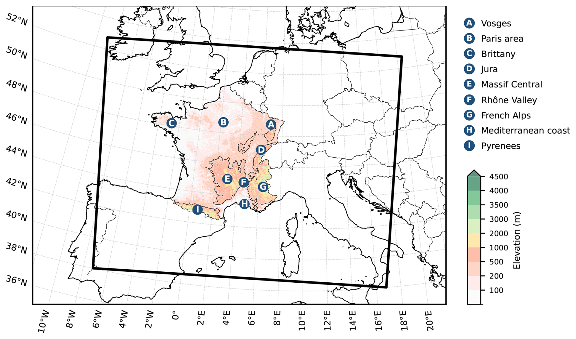
Figure 1 Map showing the computational domain of the AROME model. Shading shows topography at 2.5 km resolution and thin lines indicate the 400 m elevation contour. The letters show the geographical zones cited in the article.

The studied simulation is a 63-year AROME evaluation simulation from 1959 to 2022 directly driven by the ERA5 global reanalysis (Hersbach et al., 2020) at 2.5 km resolution. This simulation is performed over the domain ALPX-3, covering extended metropolitan France (cf. Fig. 1). The domain includes 687 × 847 grid-points, approximatively 1700 km × 2100 km, with 87 536 regularly spaced grid cells over metropolitan France. The evaluation simulation is directly driven at the domain boundaries by the ERA5 reanalysis at 50 km every hour (native ERA5 resolution ∼ 30 km). The sea surface temperatures (SSTs) are also given by the ERA5 reanalysis at 30 km resolution. Aerosols are monthly evolving and vary from year to year, taken from the ALDERA reanalysis, a CNRM-ALADIN simulation at 12 km driven by ERA5 with an interactive aerosol scheme that captures historical variations including the peak anthropogenic pollution in the 1980s and subsequent solar dimming/brightening (Nabat et al., 2020). Greenhouse gases also evolve annually.

More information on the model version and the evaluation simulation can be found in the technical note of Caillaud et al. (2026).

3 Methodology

The primary objective of this study is to validate the AROME model (grid points) against stations over metropolitan France. This is first conducted under stationary conditions to focus on the climatology (Sect. 3.1), then in a non-stationary context to assess the variability and trends in extremes (Sect. 3.2).

Evaluation is made per year, season, and month. Seasons are defined as follows: OND: October (OCT), November (NOV), December (DEC), JFM: January (JAN), February (FEB), March (MAR), AMJ: April (APR), May (MAY), June (JUN), JAS: July (JUL), August (AUG), September (SEP). The hydrological year (YEAR) is defined as the period from 1 September of year N to 31 August of year N+1. The hydrological year (September to August) is used for annual maxima instead of the calendar year, which is standard in French climatology and hydrology. This choice is motivated by the fact that the most intense extreme precipitation events in France, particularly Mediterranean episodes (e.g., Cévenol events), occur during autumn (September–November). Using a calendar year would risk splitting these autumn events across 2 years, violating the block-independence assumption required for annual maxima GEV modeling. The seasonal partition (OND, JFM, AMJ, JAS) follows the conventional grouping of months used in France for precipitation extreme studies (Haruna et al., 2026). A previous study by Berghald et al. (2025b) demonstrated that this grouping better captures trend patterns compared to the traditional seasonal definition (e.g., SON, DJF).

3.1 Climatology of extremes

While descriptive statistics such as mean precipitation or wet day frequency provide useful summaries for overall precipitation, they cannot assess quality of rare occurrence, e.g. of 10 year return events that are exceeded on average only once every 10 years. To address this limitation, we apply extreme value theory (EVT) (Coles, 2001). This states that, under general conditions, the cumulative distribution function (CDF) of block maxima – e.g. annual maxima – can be approximated by the Generalized Extreme Value (GEV) distribution.

The GEV distribution is a continuous probability distribution parameterized by the triplet $\mathit{\theta }=(\mathit{\mu },\mathit{\sigma },\mathit{\xi })$ –, respectively the location, scale (strictly positive), and shape – with the following cumulative distribution function:

$$F(x;\mathit{\mu },\mathit{\sigma },\mathit{\xi })=\exp \left\{-{\left[\mathrm{1}+\mathit{\xi }{\displaystyle \frac{x-\mathit{\mu }}{\mathit{\sigma }}}\right]}^{-\mathrm{1}/\mathit{\xi }}\right\},\mathrm{1}+\mathit{\xi }{\displaystyle \frac{x-\mathit{\mu }}{\mathit{\sigma }}}>\mathrm{0}$$

It unifies the three classical distributions Gumbel (ξ→0), Fréchet (ξ>0) and Weibull (ξ<0) where the shape parameter ξ determines the tail behavior.

The return level (or quantile of order $\mathrm{1}-\frac{\mathrm{1}}{T}$) of the GEV distribution corresponds to the threshold value exceeded, on average, once every T years. Denoting by F⁻¹ the quantile function of the GEV, it is given by:

$$\begin{array}{}\text{(1)}& \begin{array}{rl}{\text{RL}}_{\mathrm{T}}& =F^{-\mathrm{1}}\left(\mathrm{1}-{\displaystyle \frac{\mathrm{1}}{T}}\right)\\ & =\mathit{\mu }+{\displaystyle \frac{\mathit{\sigma }}{\mathit{\xi }}}\left[{\left(-\log \left(\mathrm{1}-{\displaystyle \frac{\mathrm{1}}{T}}\right)\right)}^{-\mathit{\xi }}-\mathrm{1}\right].\end{array}\end{array}$$

The GEV parameters ($\mathit{\mu },\mathit{\sigma },\mathit{\xi }$) are estimated by maximum likelihood method for each spatial location separately, considering the block maxima at a given location to be independent. This gives a set of parameters $\mathit{\mu },\mathit{\sigma },\mathit{\xi }$ and thus return level estimates from Eq. (1).

3.2 Trends in extremes

3.2.1 Non-stationary GEV models

To consider trends in extremes, the GEV distribution can be made non-stationary by allowing at least one GEV parameter to vary with time: μ(t), σ(t) and/or ξ(t). Owing to the difficulty of estimating the tail parameter ξ, it is assumed stationary, i.e. ξ(t)=ξ₀. Three non-stationary models are considered:

$$\begin{array}{c}{\displaystyle }\begin{array}{rl}& M_{\mathrm{1}}\left({\mathit{\theta }}_{\mathrm{1}}\right)\\ & {\mathit{\theta }}_{\mathrm{1}}=({\mathit{\mu }}_{\mathrm{0}},{\mathit{\mu }}_{\mathrm{1}},{\mathit{\sigma }}_{\mathrm{0}},{\mathit{\xi }}_{\mathrm{0}})\\ & \left\{\begin{array}{l}\mathit{\mu }\left(t\right)={\mathit{\mu }}_{\mathrm{0}}+{\mathit{\mu }}_{\mathrm{1}}t\\ \mathit{\sigma }\left(t\right)={\mathit{\sigma }}_{\mathrm{0}}\\ {\mathit{\xi }}_{\mathrm{0}}\end{array}\right.\end{array}\\ {\displaystyle }\begin{array}{rl}& M_{\mathrm{2}}\left({\mathit{\theta }}_{\mathrm{2}}\right)\\ & {\mathit{\theta }}_{\mathrm{2}}=({\mathit{\mu }}_{\mathrm{0}},{\mathit{\sigma }}_{\mathrm{0}},{\mathit{\sigma }}_{\mathrm{1}},{\mathit{\xi }}_{\mathrm{0}})\\ & \left\{\begin{array}{l}\mathit{\mu }\left(t\right)={\mathit{\mu }}_{\mathrm{0}}\\ \mathit{\sigma }\left(t\right)={\mathit{\sigma }}_{\mathrm{0}}+{\mathit{\sigma }}_{\mathrm{1}}t\\ {\mathit{\xi }}_{\mathrm{0}}\end{array}\right.\end{array}\\ {\displaystyle }\begin{array}{rl}& M_{\mathrm{3}}\left({\mathit{\theta }}_{\mathrm{3}}\right)\\ & {\mathit{\theta }}_{\mathrm{3}}=({\mathit{\mu }}_{\mathrm{0}},{\mathit{\mu }}_{\mathrm{1}},{\mathit{\sigma }}_{\mathrm{0}},{\mathit{\sigma }}_{\mathrm{1}},{\mathit{\xi }}_{\mathrm{0}})\\ & \left\{\begin{array}{l}\mathit{\mu }\left(t\right)={\mathit{\mu }}_{\mathrm{0}}+{\mathit{\mu }}_{\mathrm{1}}t\\ \mathit{\sigma }\left(t\right)={\mathit{\sigma }}_{\mathrm{0}}+{\mathit{\sigma }}_{\mathrm{1}}t\\ {\mathit{\xi }}_{\mathrm{0}}\end{array}\right.\end{array}\end{array}$$

Furthermore, based on previous studies that showed trends in extremes in France emerging in the mid-80s (Blanchet et al., 2018; Ribes et al., 2019; Blanchet and Creutin, 2022), we consider the case of a trend starting at year $t_{+}=\mathrm{1985}$, leading to the three models $M_{\mathrm{1}}^{\ast }$, $M_{\mathrm{2}}^{\ast }$, and $M_{\mathrm{3}}^{\ast }$. For example, in $M_{\mathrm{1}}^{\ast }$:

$$\mathit{\mu }\left(t\right)=\left\{\begin{array}{ll}{\mathit{\mu }}_{\mathrm{0}}& \text{if }t\le \mathrm{1985},\\ {\mathit{\mu }}_{\mathrm{0}}+{\mathit{\mu }}_{\mathrm{1}}(t-\mathrm{1985})& \text{if }t\ge \mathrm{1985}.\end{array}\right.$$

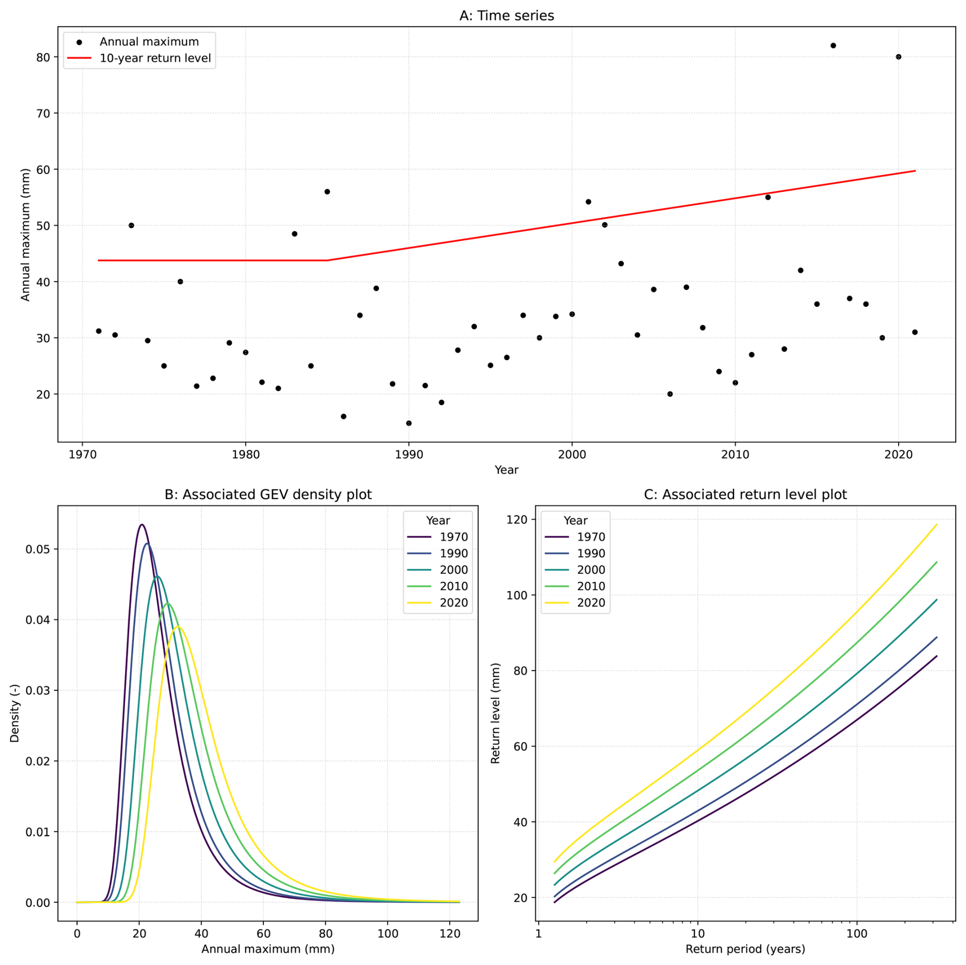
Figure 2 Influence of a trend in the μ and σ parameters for a time series of annual maxima (Example: Station 45330001 located at 48.09° N, 1.94° E). This figure illustrates an example of the $M_{\mathrm{3}}^{\ast }$ model showing a positive trend. (a) Time series (black dots) with the 10-year return level (red line); (b) GEV densities for selected years between 1970 (purple) and 2020 (yellow); (c) Associated return level curves.

Figure 2 illustrates the case of a non stationary GEV with trends in μ and σ starting in 1985 (corresponding to $M_{\mathrm{3}}^{\ast }$), with the corresponding GEV densities and associated return level plots for several years.

This gives in total six non-stationary models, in addition to the stationary model denoted (M₀), which corresponds to μ(t)=μ₀, σ(t)=σ₀, and ξ(t)=ξ₀. Although the starting year $t_{+}=\mathrm{1985}$ will be hold fixed below, considering starting year a few years before or after does not change the main results of this study (not shown).

3.2.2 Model selection

For each model, the GEV parameters θ are estimated by maximum likelihood method for each spatial location separately. At each spatial point, we thus have seven estimated models M₀, M₁, M₂, M₃, $M_{\mathrm{1}}^{\ast }$, $M_{\mathrm{2}}^{\ast }$, and $M_{\mathrm{3}}^{\ast }$ that we temporarily rename M₀ to M₆. For the hourly series (1990–2022), because all observations start after 1985, the breakpoint models M^∗ are equivalent to the standard linear models M, and the selection procedure defaults to comparing the four models M₀, M₁, M₂ and M₃. We apply for each non-stationary model M_j, j≥1, a likelihood ratio test to compare the goodness of fit of M_j to that of the stationary model M₀, accounting for their respective number of parameters to avoid overfitting. The test is based on computing the statistics ${\mathrm{\Lambda }}_j=\mathrm{2}({\mathrm{\ell }}_j-{\mathrm{\ell }}_{\mathrm{0}})$, where ℓ are the maximum likelihood values. Under the null hypothesis that the maxima are stationary, the statistics Λ_j follows a χ² with k degress of freedom, with k equal the difference in the number of parameters between M_j and M₀.

Let p_j be the corresponding p-value. If p_j ≤ 10 %, the model M_j is considered to perform better than M₀, otherwise M₀ is selected. If several models M_j are preferred to M₀, we apply the following procedure: (1) if either M₃ or $M_{\mathrm{3}}^{\ast }$ are preferred to M₀, we select among these two models that with the smallest p-value among p₃ and $p_{\mathrm{3}}^{\ast }$; (2) otherwise, we select among M₁, $M_{\mathrm{1}}^{\ast }$, M₂, $M_{\mathrm{2}}^{\ast }$ that with the smallest p-value among p₁, $p_{\mathrm{1}}^{\ast }$, p₂, $p_{\mathrm{2}}^{\ast }$.

This two-step process prioritizes models with simultaneous temporal effects on μ and σ when statistically justified, ensuring complexity is introduced only when it provides plus-value. In the rest of the article, only the selected model is considered at each location (grid point or station). However, for the evaluation of 10-year return levels as a climatological metric, we consistently rely on the stationary model (M₀).

3.2.3 Trend in return level

For a non-stationary GEV with parameters μ(t), σ(t) and ξ₀, the T-year return level is still given by Eq. (1) but it is now a function RL_T(t) of the year t. In this study, we focus on the 10-year return level (RL₁₀) as the primary metric for extreme precipitation. Our daily series (63 years) and hourly series (33 years) provide sufficient data for its robust estimation. As a sensitivity check, trends in RL₂ and RL₅ show the same regional patterns as RL₁₀ (daily: r = 0.86–0.99 among significant stations; hourly: r = 0.79–0.98), confirming that the detected signals are robust and not driven by GEV fitting uncertainty.

Owing to the linear form of μ(t) and σ(t) in the considered non-stationary models, return levels are linear functions of time in models M₁, M₂, and M₃, and linear only after 1985 in the breakpoint models $M_{\mathrm{1}}^{\ast }$, $M_{\mathrm{2}}^{\ast }$, and $M_{\mathrm{3}}^{\ast }$. In the stationary model M₀, return levels are of course constant over time. For the non-stationary models, the relative trend in the T-year return level (%) over the most recent 30-year period (between 1992 and 2022) is computed as

$$\text{RelTrend}={\displaystyle \frac{{\text{RL}}_{\mathrm{T}}\left(\mathrm{2022}\right)-{\text{RL}}_{\mathrm{T}}\left(\mathrm{1992}\right)}{{\text{RL}}_{\mathrm{T}}\left(\mathrm{1992}\right)}}.$$

It is obviously 0 if the stationary model has been selected.

3.2.4 Confidence intervals for the return levels

Noting that the T-year return level function can be written as ${\text{RL}}_{\mathrm{T}}\left(t\right)={\text{RL}}_{\mathrm{T},\mathrm{0}}+{\text{RL}}_{\mathrm{T},\mathrm{1}}t$ for models M₁, M₂, M₃ and as

$${\text{RL}}_{\mathrm{T}}\left(t\right)=\left\{\begin{array}{ll}{\text{RL}}_{\mathrm{T},\mathrm{0}}& \text{if }t\le \mathrm{1985},\\ {\text{RL}}_{\mathrm{T},\mathrm{0}}+{\text{RL}}_{\mathrm{T},\mathrm{1}}(t-\mathrm{1985})& \text{if }t>\mathrm{1985},\end{array}\right.$$

for models $M_{\mathrm{1}}^{\ast }$, $M_{\mathrm{2}}^{\ast }$, $M_{\mathrm{3}}^{\ast }$, confidence intervals for the trend coefficient RL_T,1 are obtained by profiling the likelihood with respect to RL_T,1 (Coles, 2001). If the 90 % confidence interval of RL_T,1 does not contain 0, the T-year return level trend is significant at level 10 %.

3.3 Assessing the agreement between AROME and the stations

To evaluate the CNRM-AROME model against observations, each Météo-France station is matched to the closest model grid point (2.5 km × 2.5 km) based on its geographic location. This pairing allows assessing the spatial and temporal coherence of simulated fields against raingauge measurements.

We assess the model's agreement using three main metrics:

1. Pearson correlation coefficient (r). Used to quantify the spatial consistency between observed and simulated fields across all station locations.

2. Mean Error (ME, or bias). Measures the average difference between the simulated and observed statistics, defined as:

   $$\begin{array}{}\text{(2)}& \text{ME}={\displaystyle \frac{\mathrm{1}}{n}}\sum _{i=\mathrm{1}}^n(Y_{i,\text{AROME}}-Y_{i,\text{OBS}})\end{array}$$

   where Y_i represents the climatological or trend statistic computed at station i (or its closest model grid point) and n is the total number of compared stations.

3. Relative Bias (RB, %). Expresses the bias as a percentage of the observed baseline, which is particularly useful for comparing regions with highly contrasted precipitation baselines:

   $$\begin{array}{}\text{(3)}& \begin{array}{rl}\text{RB}& =\mathrm{100}\times {\displaystyle \frac{{\sum }_{i=\mathrm{1}}^n(Y_{i,\text{AROME}}-Y_{i,\text{OBS}})}{{\sum }_{i=\mathrm{1}}^n{Y}_{i,\text{OBS}}}}\\ & =\mathrm{100}\times {\displaystyle \frac{\text{ME}}{{\stackrel{\mathrm{‾}}{Y}}_{\text{OBS}}}}\end{array}\end{array}$$

   where ${\stackrel{\mathrm{‾}}{Y}}_{\text{OBS}}$ is the mean of the observed values across all compared stations.

These metrics are calculated for five core precipitation indices: the annual frequency of wet days (daily precipitation exceeding 1 mm), the mean annual total precipitation, the daily and hourly 10-year return levels, and the relative trends in daily and hourly 10-year return levels. Climatological indices are evaluated in a stationary framework, whereas relative trends are obtained from the estimated non-stationary GEV distributions (cf. Sect. 3.2.1). In the latter case, we do not compute the relative bias as relative trends are already %.

4 Results

We begin by evaluating, grid point by grid point, the ability of AROME to reproduce the precipitation regime observed by Météo-France stations. This initial stationary evaluation allows assessing the quality of the extreme-value climatology before examining return-level trends.

4.1 Evaluation of the precipitation climatology of AROME

Figure 3 provides a spatial comparison of the precipitation climatology between AROME and Météo-France stations. In addition to the 10-year return level assessing quality of extremes, we show two descriptive statistics assessing the overall climatology of precipitation: the mean number of wet days per year (precipitation exceeding 1 mm) and the mean annual total precipitation. Across all indicators, AROME reproduces the large-scale spatial structures with high spatial correlations: matching the station locations to their closest grid points, Pearson correlation r = 0.95 for the annual frequency of precipitation days, r = 0.94 for annual cumulative precipitation, r = 0.95 for the daily 10-year return level, and a lower correlation of r = 0.78 for the hourly 10-year return level. The model correctly captures the main climatic gradients of France: dryness of the Rhône valley and the Mediterranean coast (50–70 wet days per year, annual totals no more than 550 mm yr⁻¹) contrasting with the wetness of the mountain ranges (Alps, Pyrenees, Massif Central, Vosges, Jura; 140–160 wet days per year, annual totals up to more than 1800 mm yr⁻¹). The model also reproduces the localization of the largest extremes along the Massif Central ridge and to a lesser extent in the Rhône valley and along the Mediterranean coast at both daily and hourly scales.

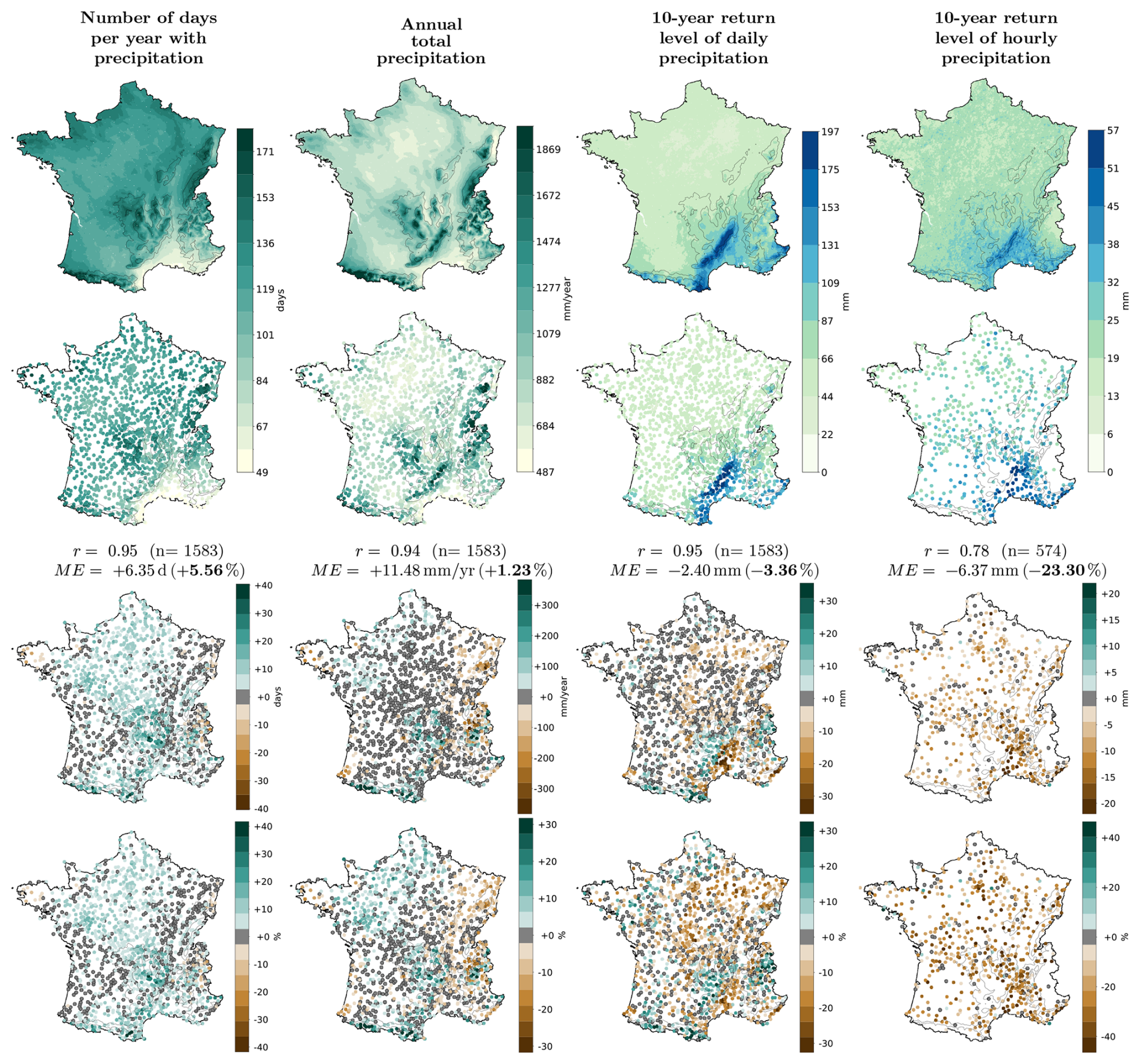
Figure 3 Climatology of the AROME simulations (first row), Météo-France stations (second row), the AROME–Station difference (third row), and the relative bias (fourth row), with the spatial correlation between the stations and their closest grid points (r), the bias (ME or relative bias RB in bold) and the number of stations compared (n). The statistics of the three first columns are derived from daily data from 1959 to 2022. The last column uses hourly data from 1990 to 2022. The contour lines show the 400 and 800 m elevation isolines. Colour scales are symmetrically saturated. Station markers have uniform size; zero bias is shown as a clearly visible grey fill.

Despite this overall agreement, the difference maps reveal structured regional biases. For precipitation frequency, AROME shows little mean bias (+6 d yr⁻¹) but local excesses above +30 d yr⁻¹ in the Massif Central and Pyrenees, while negative biases (−10 to −30 d yr⁻¹) appear in the Northern Alps, Brittany, and the Vosges. For annual cumulative precipitation, the mean bias is very small (+11 mm yr⁻¹) but regional discrepancies reach more than +300 mm yr⁻¹ along the Pyrenean ridge and Northern Alps, and −100 to −400 mm yr⁻¹ from the Northern Pré-Alps to the Vosges. For daily 10-year return level, AROME shows almost no mean bias (−2 mm) but it spreads the extremes too widely around the Massif Central ridge, giving local deficits of −10 to −20 mm along the ridge where the station extremes are the largest and +10 to +30 mm over the Massif Central Plateau. Overestimation is also visible in the Northern Alps and the Pyrenees. At the hourly scale, AROME strongly underestimates the 10-year return levels (−6.37 mm, −23.30 %), with widespread deficits of −5 to −20 mm over most of France, especially in the southern Massif Central and the Rhône Valley.

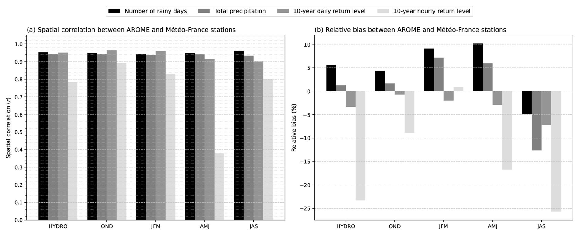
Figure 4 Seasonal synthesis of the climatological agreement between the AROME simulations and Météo-France stations for the four precipitation indices: (a) spatial Pearson correlation (r) and (b) relative bias (RB, in %) depending on the season.

The good performance of AROME for the frequency of wet days, the annual precipitation and the daily extremes is found across all seasons (see Fig. 4 for an overall view and Figs. A1 and A2 for seasonal maps of extremes), despite a slight loss in performance in spring and summer for the extremes (AMJ to JAS, correlation around 0.9). Performance is lower for hourly extremes across all seasons and particularly in spring where correlation drops to 0.38.

In summary, AROME shows a good representation of the climatology of precipitation extremes that encourages us to continue evaluation on trends, keeping however in mind that hourly extremes are systematically underestimated by the model throughout the year (especially during spring and summer) and exhibit a lower spatial agreement in spring.

4.2 Evaluation of extreme precipitation trends

4.2.1 Daily

At the hydrological year scale, the stationary model is selected for about two-thirds of the stations. For the remaining one-third, significant changes in the GEV distributions are observed, with nearly equal proportions of linear trend model (M) and breakpoint models (M^∗). AROME model exhibit similar proportions. At the seasonal scale, the only notable difference occurs in winter, where the linear model is slightly more frequent than the breakpoint model (22 % vs. 13 %). Before analyzing trends in daily return levels, we verified the consistency of GEV-estimated trends in the mean against those obtained via a simple linear regression on observed annual maxima. This preliminary check shows a very strong spatial and quantitative agreement (Pearson correlation r = 0.86 for absolute trends, r = 0.88 for relative trends), confirming the robustness of the statistical fits.

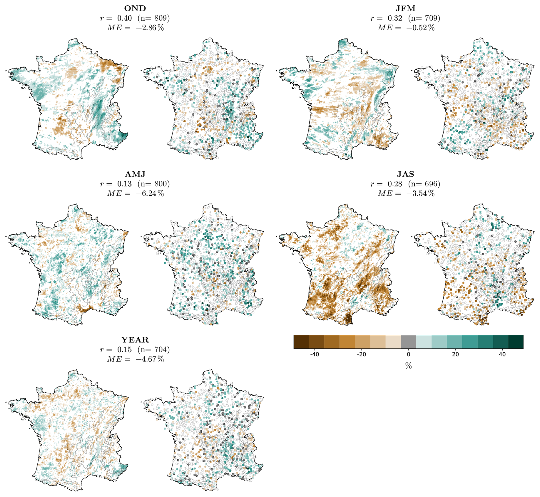
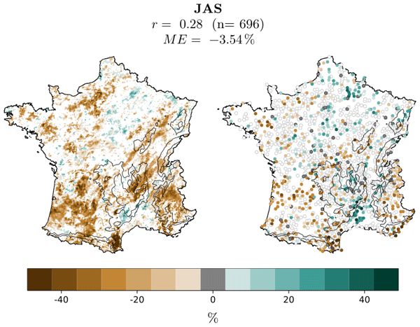
Figure 5 Relative trends over 1959–2022 (%) in the 10-year return level of daily precipitation for AROME (left) and Météo-France stations (right). Display conventions: non-significant stations as open circles (white fill); significant trends close to zero as filled grey (dark outline); significant non-zero trends coloured on the map scale (uniform marker size); non-significant AROME grid cells not displayed. Metrics (r, n, ME) are computed on significant trends only.

At the daily scale, station-based trends in the 10-year return level (Fig. 5) show spatially coherent but region-dependent signals across France over 1959–2022. For the hydrological year (YEAR), we see a clear reinforcement along the Rhône Valley (+5 % to > +30 %) and in the southern Alps (+20 % to +30 %). Elsewhere, trends are weak, of mixed sign, and often not significant, supporting a seasonal breakdown. Autumn (OND) shows a similar pattern in trends as the annual scale, with the exception of the Paris area that shows a decrease (−5 % to −20 %). In winter (JFM), France is cut in three with a diagonal of decrease from the Mediterranean coast to the Atlantic coast (−10 % to −40 %) and mainly increases elsewhere. Spring (AMJ) is characterized by a more spatially uniform positive trend over much of the country, with local increases exceeding +35 %. Summer (JAS), shows predominantly negative trends in the southern half of France, apart in the Rhône valley, with an accentuated decrease along the Mediterranean coast (up to −40 %) and mainly positive trends in the northern half.

AROME reproduces the broad spatial organization of these daily-scale patterns but generally underestimates their amplitudes (negative bias). For the hydrological year, the model partly captures the significant increase in the Southern Alps, albeit with weaker intensities, and does not reproduces the Rhône Valley reinforcement observed in the stations. Autumn is the season when trend patterns are best represented (r=0.40). AROME correctly identifies the positive signal in the Rhône valley and the negative trends in the Paris area, although it barely sees the decrease in the northern Alps. In winter, the model barely retrieves the diagonal of decrease from the Mediterranean to the Atlantic coast and it misses the decrease over the Alps. All the largest trends are anyway less marked. In spring, AROME produces weak and poorly organized signals and fails to reproduce the widespread positive trends measured by the stations. In summer, the model correctly identifies a general negative tendency over the souther half of France but does not see the increase over the Rhône valley and the northern half of France. Overall, AROME moderately captures the large-scale signs and structure of daily return-level trends but tends to underestimate both their intensity and spatial coherence.

4.2.2 Hourly

Similarly to the daily scale, we verified the consistency of GEV hourly trends by comparing GEV-estimated trends in the mean to linear regression trends of observed annual maxima. Despite the shorter record length and the higher noise level of sub-daily extremes, we find a robust agreement (Pearson correlation r = 0.72 for absolute trends, r = 0.70 for relative trends).

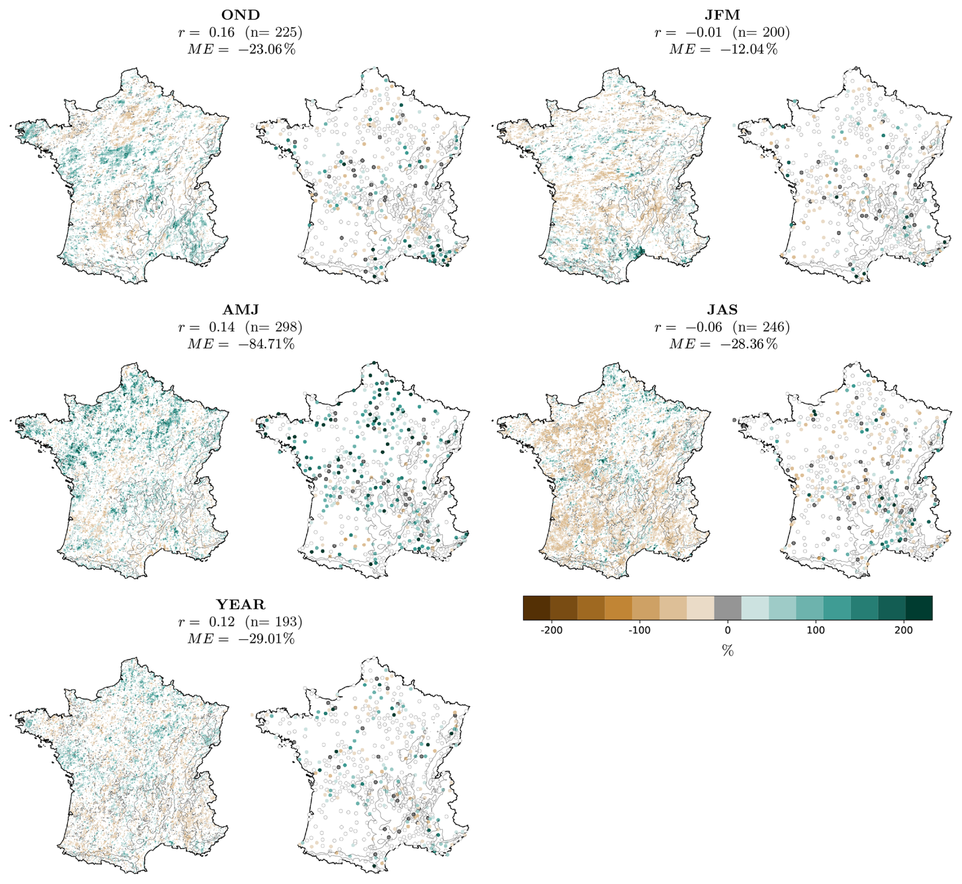
Figure 6 Relative trends over 1990–2022 (%) in the 10-year return level of hourly precipitation for AROME (left) and Météo-France stations (right). Display conventions: non-significant stations as open circles (white fill); significant trends close to zero as filled grey (dark outline); significant non-zero trends coloured on the map scale (uniform marker size); non-significant AROME grid cells not displayed. Metrics (r, n, ME) are computed on significant trends only, with 90 % colour-scale saturation.

At the hourly scale (Fig. 6), station-based trends in the 10-year return level over 1990–2022 are markedly more heterogeneous, noisy, and locally more extreme than their daily counterparts (Fig. 5), with significant trends ranging $[-\mathrm{50}\mathit{\%},+\mathrm{100}\mathit{\%}]$ versus $[-\mathrm{30}\mathit{\%},+\mathrm{30}\mathit{\%}]$ at the daily scale. Most of the significant trends are highly positive. Though noisier than at daily scale, these trends are robust in the sense that they are not produced by a single year. Removing the overall maxima of each station and fitting the GEV distributions on these new series gives slightly lower trends for the positive trends and slightly larger trends for the negative ones (Fig. B1) – which was expected since the largest value is omitted – but the magitudes and patterns remain close. Over the hydrological year, no clear spatial pattern of trends is found apart in few isolated stations where trends reach ± 50 % and occasionally exceed +100 %. At the hydrological year scale, the stationary model M₀ is selected for 74.2 % of the stations, and standard linear trend models (M) for 25.8 % (compared to 75.1 % and 24.9 % for the AROME simulations, respectively). Seasonally, the signals remain highly contrasted. In autumn, a pronounced positive pattern emerges along the Mediterranean coast, locally approaching +100 %. In winter, no clear spatial pattern of trends is found apart at some isolated stations spread over western France, the eastern Pyrenees and the Rhône valley, where strong increases of up to +100 % are found. Spring is the only season when a quite coherent pattern is found. Stations exhibit widespread and very strong increases across much of the country, frequently above +60 % and locally approaching +100 %. In summer, spatial variability reaches its maximum, with trends spanning the full range from −100 % to +100 %, particularly in the Rhône Valley. These patterns reflect both the strong local variability of convective extremes and the limited length of the hourly record, which jointly hinder the emergence of a clear regional-scale climate signal.

AROME only partially reproduces these hourly-scale patterns. Across all seasons, the model simulates weak and spatially inconsistent signals and fails to capture the most pronounced positive trends seen in the station data. For the hydrological year, spatial correlation between AROME and stations remains low (r ≈ 0.12), and seasonal correlations are close to zero for several seasons. Mean biases are substantial and of varying sign, with values reaching ME = −84.7 % in spring and ME = −28.4 % in summer. While AROME occasionally recovers the sign of the observed trends in some regions, it generally does not reproduce their fine-scale spatial organization or amplitude.

4.2.3 Monthly refinement

The monthly analysis (Fig. 7) further highlights the specificity of convective regimes and the strong temporal concentration of some signals. Figure 7a compares the monthly median GEV relative trends at Météo-France stations and the corresponding AROME grid points (side-by-side subpanels). At the daily scale, station median trends remain moderate throughout the year, ranging from −16.27 % in September to +14.05 % in April/May. In contrast, station-based hourly GEV trends show far larger values concentrated in specific convective windows, with monthly medians reaching +43.28 % in February, +28.26 % in March, +101.86 % in June, +53.88 % in October, and +30.09 % in December. AROME reproduces the positive sign of these monthly trend peaks but systematically underestimates their magnitude. For instance, in June, AROME simulates a median hourly GEV trend of +17.70 % (against +101.86 % for stations), and in February, it simulates +11.46 % (against +43.28 % for stations).

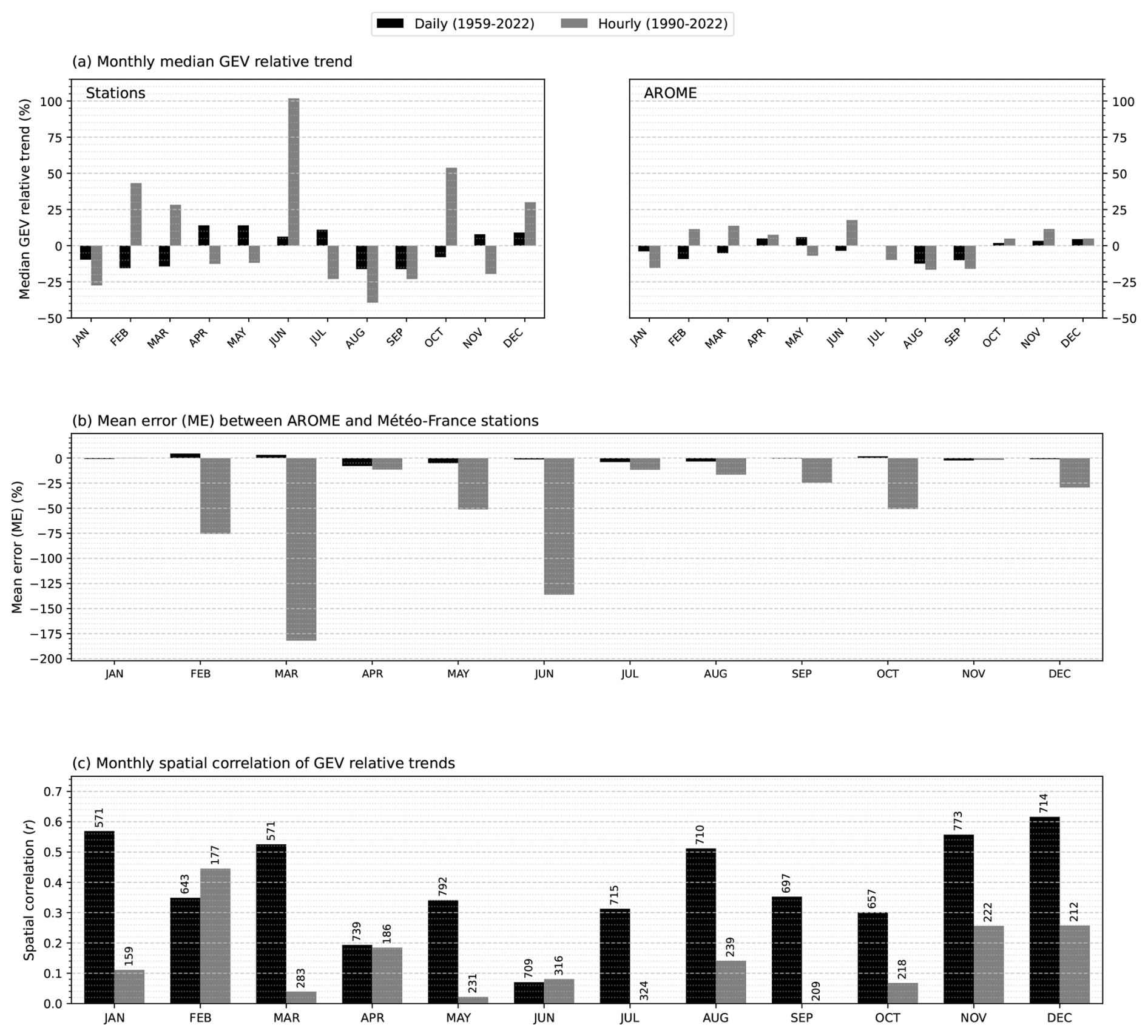
Figure 7 Monthly GEV relative trend synthesis for both daily (1959–2022) and hourly (1990–2022) scales, calculated only over locations with statistically significant trends at the stations (at the 10 % level): (a) median GEV relative trend (%) at Météo-France stations (left) and corresponding AROME grid points (right); (b) mean error (ME, in %) between the relative trend of the corresponding AROME grid points and Météo-France stations; and (c) spatial correlation (r) of GEV relative trends. Values above each bar in panel (c) indicate the number of significant stations used in the calculations. All statistics are evaluated at AROME grid points corresponding to these stations.

This systematic underestimation is reflected in the monthly mean errors (ME) between the stations and the corresponding AROME grid points shown in Fig. 7b, with large negative values at the hourly scale during convective months (e.g., ME = −75.6 % in February, ME = −182.0 % in March, and ME = −136.1 % in June), whereas daily mean errors remain much smaller (e.g., ME = −0.9 % in January and ME = 3.1 % in March).

Finally, Fig. 7c shows that spatial correlation (r) is consistently higher at the daily scale (peaking at r = 0.62 in December) than at the hourly scale. At the hourly scale, spatial correlations are extremely low or close to zero during the convective months (e.g., r = 0.08 in June, r = 0.07 in October, r = 0.04 in March, and r = 0.02 in May), and virtually zero in July and September (r ≈ 0.00), reflecting the high local spatial variability of hourly trends. February stands out as the only month showing moderate spatial agreement (r = 0.45). The detailed monthly spatial patterns of hourly GEV trends are presented in Appendix C (Fig. C1).

5 Discussion

5.1 Limitations of the study

This study provides the first evaluation of the AROME simulations for reproducing trends in extremes in France. The evaluation is based on a comparison with rain gauge data, considered here as the reference, which induces some limitations that we list below.

5.1.1 Temperature trends

It should be noted that temperature trends (cf. Fig. 8) with the AROME model forced by ERA5 are about one-third weaker than observed trends. This implies a dampening of the Clausius–Clapeyron-related component of extreme precipitation trends, which is expected to influence the magnitude of the trends we can detect.

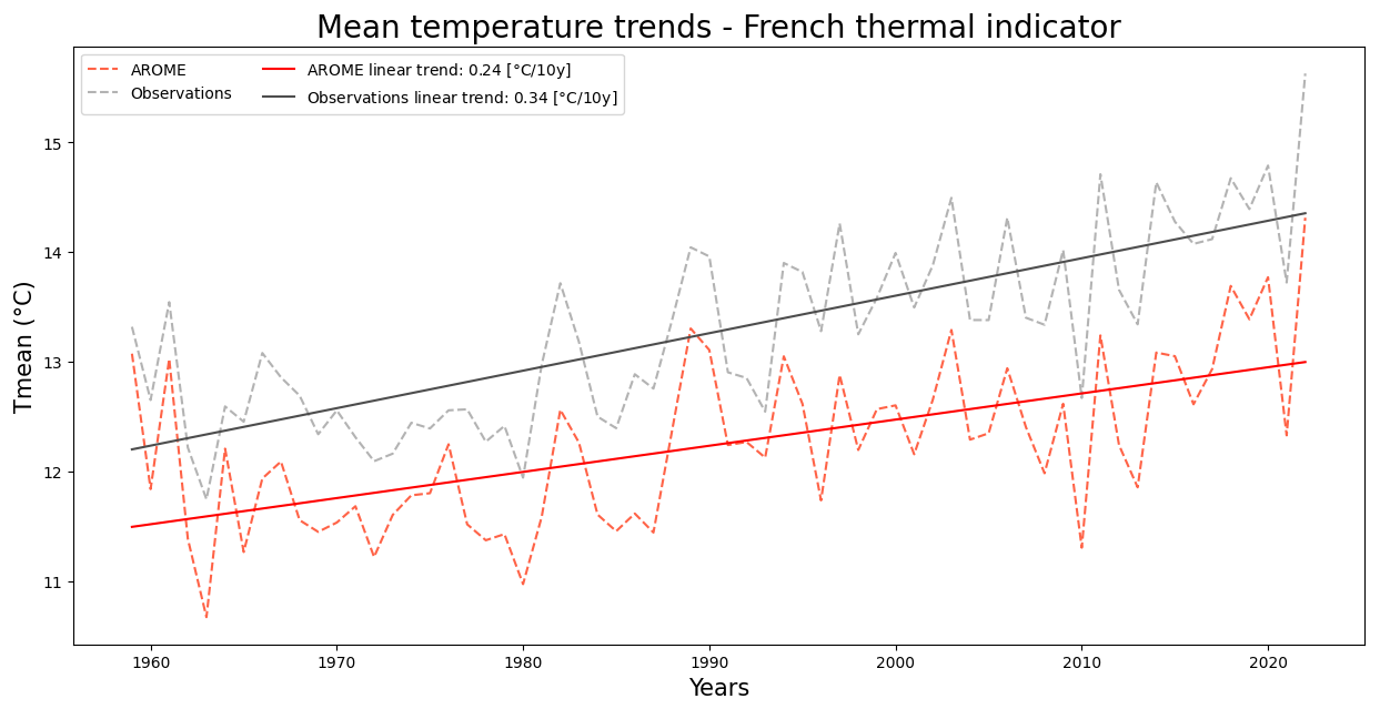
Figure 8 Temporal evolution of the annual mean temperature between 1959 and 2022. For the observations, the time-series are computed from the French thermal indicator, i.e. the mean of a given set of 30 stations with homogenised data, which are the reference temperature stations in France (Gibelin et al., 2014). For the model, the time-series are computed over the mean of the 30 grid-points that are the closest to the stations. For each time-series, the trend is computed using a linear regression.

The weaker simulated temperature trend suggests an internal dampening of the warming signal in France compared to observations. Since aerosols and greenhouse gases evolve realistically in this simulation (Sect. 2.2) and ERA5 reproduces observed temperature trends well (Hersbach et al., 2020), the underestimation likely stems from the model's internal sensitivity to radiative forcings, the absence of interactive vegetation, and/or the lack of temporal evolution of the land use/land cover map.

5.1.2 Data

First, station precipitation measurements are frequently affected by undercatch errors, which are particularly pronounced in cold and mountainous regions with strong winds. Since undercatch typically results in an underestimation of actual precipitation – especially for high-intensity, short-duration convective events–, correcting these errors would increase the observed extreme values. Consequently, the model's underestimation of hourly extremes is likely even larger than what we report here. Part of this underestimation may also stem from the 2.5 km horizontal resolution of AROME: Brousseau et al. (2016) showed that increasing the resolution to 1.3 km results in a better representation of maximum precipitation intensities, with less pronounced underestimation. Furthermore, station time series can also exhibit some inhomogeneities (non-climatic shifts in the time series caused by changes in station location, environment, or sensor types over decades), which could introduce local artificial trend components, although the data used here have been quality-controlled by Météo-France.

Second, raingauges provide measurement over short periods, particularly the hourly data that are available since the 1990s only. This is particularly problematic when studying extremes within a GEV framework, as only one value (the maximum value) is used per year. In some cases, isolated outliers can significantly influence estimates of the return level (Zeder and Fischer, 2024). For example, in Fig. 6, some individual points stand out from their surroundings, which is probably due to sampling bias and not to differences in climate. To make the estimation more robust, other solutions include taking into account threshold exceedances within a generalized Pareto distribution (GPD) framework, or using a distribution modeling all precipitation values, such as the recent extended generalized Pareto distribution (Haruna et al., 2025) or the Simplified Metastasis Extreme Value (SMEV) distribution (Marra et al., 2020; Correa-Sánchez et al., 2025; Lompi et al., 2025), or using a neighborhood or region-of-influence approach (Blanchet et al., 2021) to reduce sampling bias by using more data. All these methods have their advantages and disadvantages. Our general advice is not to interpret trends at an individual point, but to look for consistent trends across regions, to avoid over-interpretation.

Third, the stations are not evenly distributed across the country. In particular, hourly stations are lacking in the Alps, the Pyrenees and, to a lesser extent, the Massif Central. This naturally has an impact on our evaluation measures (correlation and bias) and prevents us from fully evaluating AROME in mountainous regions.

5.1.3 Evaluation scheme

A limitation of the evaluation is that it compares point-scale raingauge measurements with 2.5 km × 2.5 km AROME grid-box averages. This mismatch in spatial support is relatively modest for daily accumulations, but it becomes a major limitation at the hourly scale: a single convective core may affect only part of a grid cell, so that local station extremes can be much higher (or lower) than the corresponding AROME value even when the event is realistically simulated at the grid-box scale. A high-resolution gridded observational product would therefore be better suited to evaluating hourly extremes than individual stations. In this respect, Météo-France’s COMEPHORE product – a 1 km, hourly radar-gauge precipitation reanalysis over metropolitan France – would be particularly valuable (Météo-France, 2025b). It would have been interesting to include COMEPHORE in this study, but the reanalyses only begin in 1997 and the method for calculating the rainfall fields changed in 2007, which could affect trend estimation.

5.1.4 Statistical modeling framework

Another limitation stems from the modeling framework. We have applied a non-stationary GEV framework to estimate trends in extremes. This requires more parameters to be estimated and additional assumptions to be made about the shape of the trends. Here, we have assumed that the distribution of parameters, and therefore return levels, evolve linearly over time. This is obviously a simplification, as (i) there is no physical reason for the evolution to be linear, (ii) there is no direct physical dependence between return levels and time. The linearity assumption could be relaxed by considering non-linear transfer functions (e.g. power functions), with the risk of over-fitting and increased uncertainty if more parameters have to be estimated. Here, as in many other studies based on GEV distributions, we prefer to use a rigid (linear) relationship to increase robustness. Previous studies analyzing the relationship between temperature and precipitation (Da Silva and Haerter, 2025) lead us to believe that temperature might be a more appropriate covariate. However, which temperature to choose and at which scale (e.g. local temperature at the time of the event, annual region-mean temperature, sea-surface temperature) is a matter of debate in itself (Schröer and Kirchengast, 2018; Dash and Maity, 2023; Zeder and Fischer, 2020), which is why we chose to keep time as the simplest covariate. Temperature change over the recent past is anyway close to linear in time, so we believe that the magnitude of the trends would be barely affected.

5.2 Climatology: consistencies and divergence

The results confirm that AROME correctly reproduces the main rainfall regimes over metropolitan France, as supported by the literature (Fumière et al., 2020; Caillaud et al., 2021; Dura et al., 2024; Lucas-Picher et al., 2024b; Cortés-Hernández et al., 2024). It is able to reproduce the climatological orographic intensification of precipitation over the Alps, the Pyrenees, and the Massif Central, a pronounced transition from Atlantic to continental climatic influence in the west, and the dryness of the Mediterranean basin. This consistency with the stations indicates a satisfactory representation of the dynamical forcings (moisture transport by westerly flows, orographic uplift, low-level circulation in the Mediterranean).

AROME's ability to reproduce the frequency and quantity of precipitation and the 10-year return level of daily precipitation is maintained throughout the year. Performance declines for the 10-year return level hourly precipitation specialy in spring (r = 0.38). Studies with the previous version of the model show that AROME underestimates high-intensity precipitation (> 40 mm h⁻¹) (Caillaud et al., 2021; Poncet et al., 2024). Summer convection remains partially under-resolved despite the 2.5 km spatial resolution. Running AROME at finer resolution might improve this, as it was shown that a 1.3 km resolution results in a better representation of maximum intensities (Brousseau et al., 2016). A separate analysis (not shown) shows that correlation increases (+30 %) for 6 and 9 h precipitation. One can hypothesize that AROME spreads convective precipitation too widely in time and in space over nearby grid points, giving underestimated local peak precipitation. Unfortunately this hypothesis cannot be fully evaluated given the sparse station network.

5.3 Trends in precipitation extremes: consistencies and divergence

5.3.1 Daily data: confirmation of known patterns and model–observation consistencies

The daily trends derived from Météo-France stations confirm and refine previously documented spatial structures of extreme-precipitation evolution in France. The significant increases in the Rhône Valley and the southern Alps (+5 % to +30 %) are fully consistent with earlier regional analyses reporting an intensification of daily extremes in southeastern France (Blanchet et al., 2018, 2021; Ribes et al., 2019). The marked increases detected in northern France (locally up to +35 %) also agree with national-scale projections indicating a northward-shifted reinforcement of daily extremes under strong warming scenarios (Soubeyroux et al., 2025). The weak or non-significant trends observed across large parts of western and central France likewise corroborate the high spatial variability highlighted in the IPCC report (IPCC, 2021).

Overall, AROME reproduces the main spatial structures and magnitudes reasonably well when compared with the station-based climatology. The model correctly identifies regions of positive change (southern Alps, Rhône Valley, parts of northern France) and regions with weak or negative signals (western France, the Paris area), indicating an overall ability to capture the pattern of daily return-level evolution. However, AROME systematically underestimates the amplitude of the trends. This reduced magnitude is consistent with the underestimation of temperature trends in AROME that is about one-third weaker than observed trends (Fig. 8).

5.3.2 Hourly data: new national-scale findings and limited model-observation consistency

Unlike the daily scale, no national mapping of hourly 10-year return-level trends has previously been available for France. The present work therefore provides the first nationwide characterization of hourly extreme-precipitation trends, offering new insight into their spatial organisation.

Over 1990–2022, trend magnitudes in hourly extremes frequently reach ± 50 % and can exceed +100 %, with strong seasonal dependence. Coherent monthly signals emerge nonetheless: February trends in the Rhône Valley, March trends along the western Mediterranean arc, November increases in the eastern Mediterranean arc, and widespread June increases across most of France. These patterns, though noisier than daily trends, are robust in the sense that they are not produced by a single year (Fig. B1). This indicates the start of an emerging trend in hourly extremes even within the constraints of a relatively short observational period.

AROME reproduces part of the seasonal structure of these hourly signals – concurring on the months associated with enhanced extreme activity (Fig. 7a) – but fails to capture their spatial organization and magnitude. The model systematically underestimates the magnitude of positive hourly GEV trends, leading to a much larger underestimation of relative trends at hourly than at daily scale (e.g., ME = −136.1 % vs. −1.4 % in June, see Fig. 7a and b). Furthermore, hourly spatial correlations remain close to zero for most convective months (e.g., r = 0.08 in June and r = 0.04 in March, see Fig. 7c), reflecting shifts in the simulated convective precipitation zones, especially in mountain regions (such as the Massif Central and the Alps) where summer convective activity dominates. Part of this trend magnitude underestimation is consistent with the underestimation of temperature trends in AROME (Fig. 8).

Overall, the hourly results highlight two major conclusions: (i) the station-derived hourly trends presented in this study constitute a new contribution to the climatology of French precipitation extremes, revealing structured yet highly localized patterns; (ii) AROME currently shows limited skill in representing both the magnitude and spatial heterogeneity of hourly return-level trends, even when significant signals are isolated, underscoring the challenges of simulating sub-daily extremes.

6 Conclusion

This study evaluated the ability of the convection-permitting regional climate model AROME (2.5 km), forced by ERA5 over 1959–2022, to reproduce the climatology and the recent evolution of extreme precipitation in metropolitan France, using Météo-France rain-gauge observations at daily (1959–2022) and hourly (1990–2022) time scales. Extremes were characterized using statistical GEV distributions (stationary and non-stationary), and trends were quantified through changes in 10-year return levels.

Overall, the AROME simulations provide clear value for the climatology and the spatial organization of daily extremes, and they can support national-scale analyses of daily extreme-precipitation changes, provided that trend magnitudes are interpreted cautiously. In contrast, the evaluation indicates that hourly return levels and especially their trends are less well reproduced, with hourly trends almost inexistent in AROME. However our evaluation shows limitation at hourly scale due to spatial support mismatch between stations and grid points, and short observational record length of stations that prevented us from making the comparison over the full 1959–2022 simulation period. Future work should rely on high-resolution gridded reference datasets (e.g. radar–gauge reanalyses) to reduce representativeness errors and investigate the sensitivity of results to temporal and spatial aggregation (multi-hour maxima, intensity-duration-area-frequency curves, Haruna et al., 2024. These steps are necessary to assess the reliability of CNRM-AROME simulations' representation of extremes, and to pave the way for its use in studying extremes in climate projections.

Appendix A: 10-year return level of precipitation

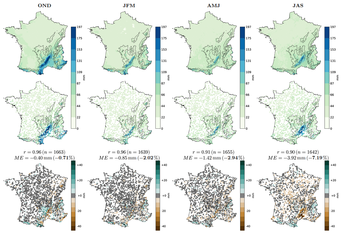
Figure A1 10-year return level of daily precipitation of the AROME simulations (first row), Météo-France stations (second row), and the AROME–Station difference (third row), with the spatial correlation between the stations and their closest grid points (r), the bias (ME) and the number of stations compared (n). The statistics are derived from daily data from 1959 to 2022. The contour lines show the 400 and 800 m isolines. To ease visualization, colour scales are symmetrically saturated above the 99th percentile.

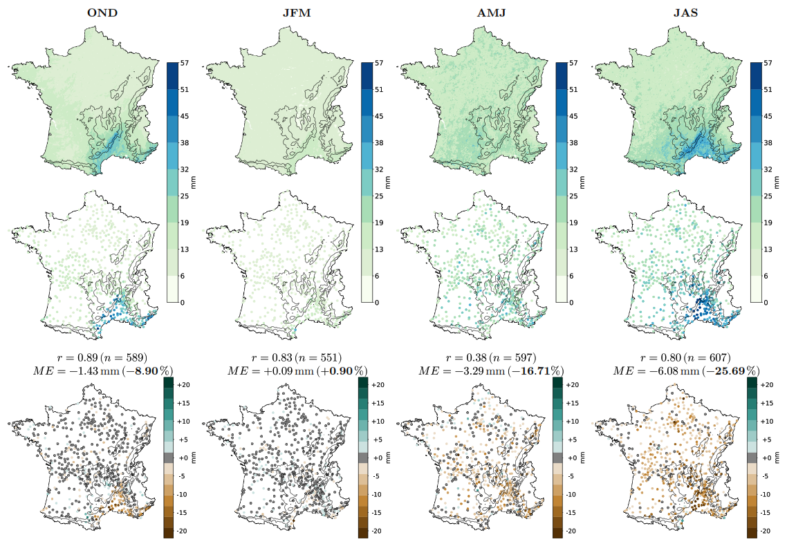
Figure A2 10-year return level of hourly precipitation of the AROME simulations (first row), Météo-France stations (second row), and the AROME–Station difference (third row), with the spatial correlation between the stations and their closest grid points (r), the bias (ME) and the number of stations compared (n). The statistics are derived from daily data from 1990 to 2022. The contour lines show the 400 and 800 m isolines. To ease visualization, colour scales are symmetrically saturated above the 99th percentile.

Appendix B: Robustness of trends when discarding the overall maxima

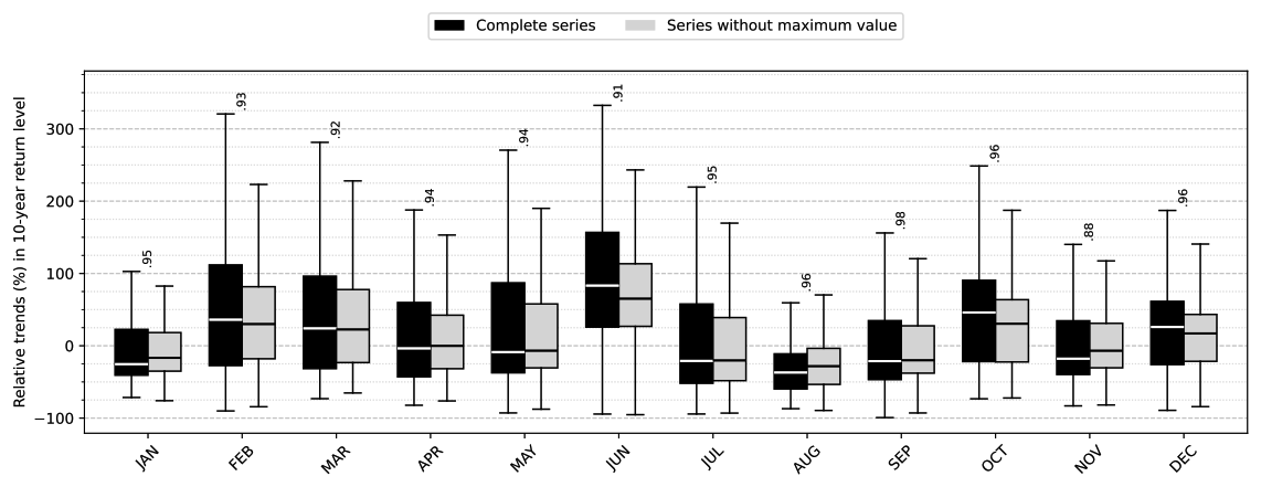
Figure B1 Relative trends over the last thirty years ending in 2022 (%) in the 10-year return level of hourly precipitation for Météo-France stations when considering the complete series (left) and when discarding the overall maximum (right). Only the the stations with significant trends (for the complete series) are used. The numbers written above each month indicate the Pearson correlation (r) between trends of the complete series and trends of the series without the overall maximum.

Appendix C: Monthly trend maps of hourly extremes

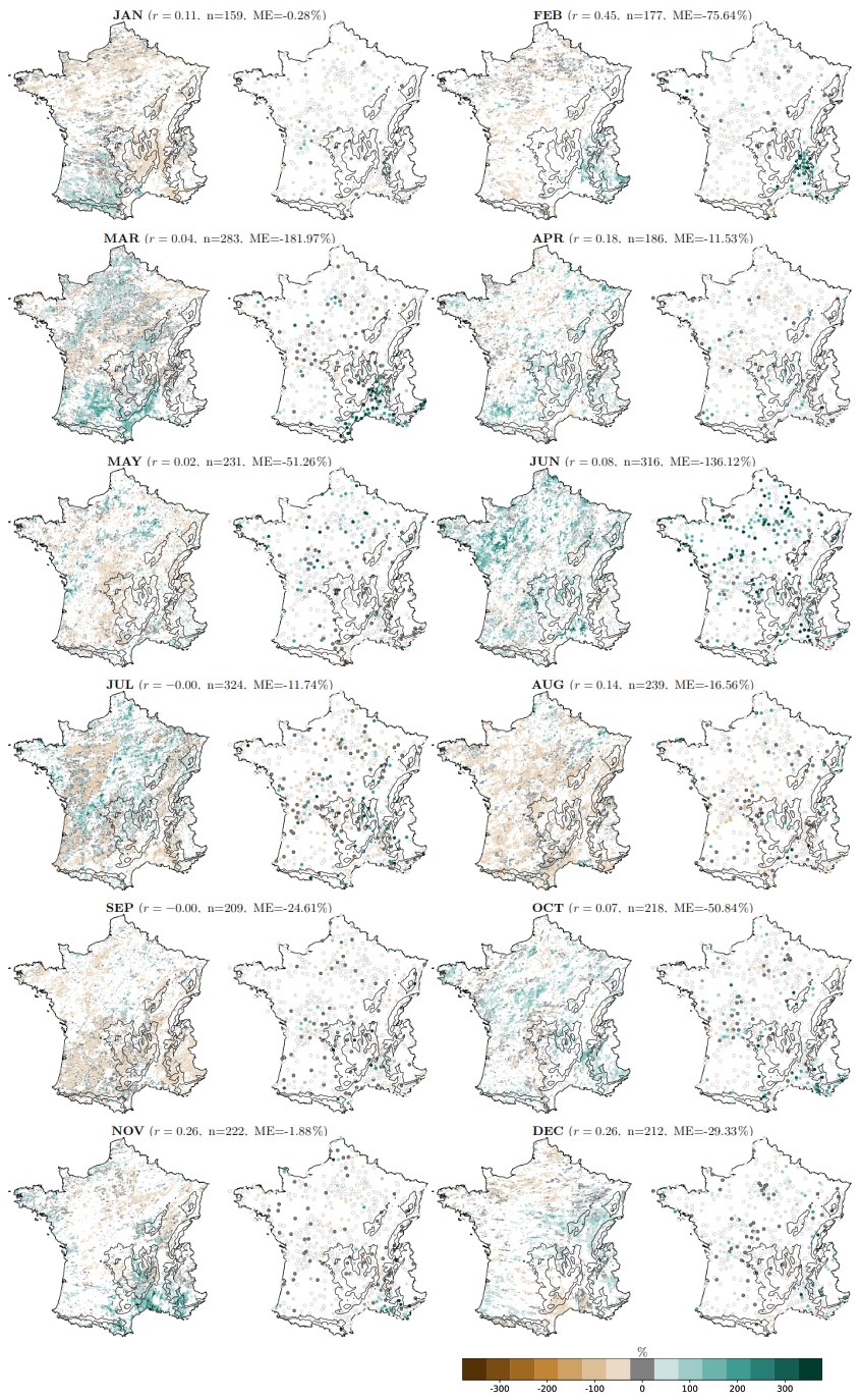
Figure C1 Relative monthly trends over 1990–2022 (%) in the 10-year return level of hourly precipitation for AROME (left) and Météo-France stations (right). Display conventions: non-significant stations as open circles (white fill); significant trends close to zero as filled grey (dark outline); significant non-zero trends coloured on the map scale (uniform marker size); non-significant AROME grid cells not displayed. Metrics (r, n, ME) are computed on significant trends only.