Climate and landscape jointly control European streamflow behaviour

The complex composition of hydrological systems, climates and landscapes makes it challenging to explain and predict hydrological streamflow response. Many previous large-sample studies, mostly focused on the United States, identified climate as the primary control, with landscape exerting only a minor role in shaping hydrological behaviour. Yet, a few other studies report contradictory results with landscape being a more dominant driver. In this study, we use an unprecedented sample of more than 7000 catchments in Europe from the EStreams dataset to identify and map functionally similar catchments, together with their spatially variable climate and landscape controls. The wide spatial and temporal gradient of the study catchments was used to identify hydrological response types (HRTs) based on 40 hydrological streamflow signatures related to long-term averages and inter-annual variability of magnitude, timing, duration, frequency, and seasonality. Overall, 10 HRTs could be identified. Several HRTs are well defined and well distinguishable, largely due to catchments with strongly seasonal or more extreme behaviour. Other HRTs remain difficult to distinguish, as these catchments represent more transitional conditions with increasingly overlapping characteristics between HRTs. The underlying drivers of the HRTs were identified by using 84 climate- and landscape attributes to predict catchment membership to their respective HRT with a Random Forest classification model. Climate emerges as the dominant driver of hydrological behaviour at the continental scale. However, landscape was found, in 4 out of 10 HRTs, to be at least as strong or even stronger a control on the hydrological streamflow response. These results highlight that the complex, integrated nature of hydrological response remains challenging to disentangle, even with extensive datasets and advanced modelling approaches, and therefore, climate and landscape need to be understood as joint drivers in a co-evolutionary perspective.

1 Introduction

In terrestrial hydrological systems, the landscape acts as a low-pass filter that buffers precipitation water input before it is released from the system as streamflow or evaporation. The magnitude and dynamic changes of streamflow over time are thus a manifestation of the combined and aggregated effects of the hydro-climatic characteristics and the physical properties of the landscape in a catchment. Any catchment is characterised by a heterogeneous mosaic of countless local landscape features that each influence the movement of water in different ways (Beven, 2000; Sivapalan, 2003a; Wagener et al., 2007). In practice, these controls are inherently intertwined, as climatic inputs are mediated through landscape properties such as topography, soils, geology, vegetation and storage elements before contributing to streamflow. The combination of the hydro-climatic characteristics with these local landscape elements and their topology in any catchment is a multivariate fingerprint that may be considered unique (Beven, 2000). In spite of this potential “uniqueness of place” (Beven, 2000) and the associated spatial complexity of the hydrological response, there is evidence that self-organisation leads to relatively simple hydrological response patterns that emerge at larger scales (e.g. catchment-scale) and that can be relatively well quantified using various streamflow signatures. The latter are index values derived from streamflow observations that describe catchment characteristics such as magnitude, seasonality and flashiness. Common examples include mean flow, baseflow index or the slope of the flow duration curve (FDC) (McMillan et al., 2017). Hydrological signatures provide interpretable metrics that facilitate the identification of similarity, response patterns and dominant processes across catchments. Systematically mapping catchment-scale hydro-climatic and landscape attributes against catchment-scale hydrological response patterns then holds the potential to identify hydrological (dis)similarities across catchments in diverse environments and to classify them into types with distinct hydrological functioning (Dooge, 1986; Blöschl, 2006; Wagener et al., 2007; McDonnell et al., 2007). Such a classification is critical to inform the design of architectures and parametrisations of hydrological models (Gupta et al., 2014), as demonstrated by several studies (e.g., Merz and Blöschl, 2004; Parajka et al., 2005; Ye et al., 2012; Fenicia et al., 2014; Beck et al., 2020; Dal Molin et al., 2020). The increasing number and volume of large-sample datasets (e.g., Addor et al., 2017; Gudmundsson et al., 2018; Fowler et al., 2021; Kratzert et al., 2023; do Nascimento et al., 2024) in hydrology has over the past two decades facilitated ever more detailed comparison, classification and regionalisation studies which led to considerable progress in that direction (e.g., Merz and Blöschl, 2003, 2009; Laaha and Blöschl, 2006a, b; Carrillo et al., 2011; Sawicz et al., 2011; Coopersmith et al., 2012; Yaeger et al., 2012; Berghuijs et al., 2014; McManamay et al., 2014; Beck et al., 2015; Kuentz et al., 2017; Addor et al., 2018, 2020; Knoben et al., 2018; Brunner et al., 2020; Almagro et al., 2024; Brêda et al., 2024; He et al., 2024; van Oorschot et al., 2024; Vu et al., 2024; Slater et al., 2024; do Nascimento et al., 2025a; Araki et al., 2026).

These studies exhibit substantial variation in terms of both the number of catchments analysed and the methodological choices employed in the classification. While some studies have classified on climatic characteristics (Knoben et al., 2018; Brunner et al., 2020), streamflow signatures (Kuentz et al., 2017; Almagro et al., 2024) or on a combination of the two (Kemter et al., 2023), others have considered landscape attributes only (Jones et al., 2021). For example, Berghuijs et al. (2014) used three elements of the seasonal water balance to group catchments in the U.S. Based on the coherent similarity of streamflow signatures within the formed groups, they could conclude that climate is the dominant driver of streamflow variability. This broadly corresponds with the results of Kuentz et al. (2017), who used 16 flow signatures to group 1366 catchments into 11 functionally distinct groups across Europe. Further analysis of these groups against 35 climate- and landscape attributes revealed that most signatures were controlled by climatic factors. Using Random Forest models to predict a range of hydrological signatures (Addor et al., 2018) and regime types (Brunner et al., 2020) of 671 U.S. catchments, suggested that climate attributes were the most important predictor, with landscape attributes playing only a minor role.

Somewhat more nuanced results were reported by Almagro et al. (2024), who classified more than 700 Brazilian catchments into six groups based on their hydrological similarity and analysed which climate- and landscape attributes were the most influential on individual hydrological signatures within these groups. Although climate was, for the majority of the six groups, the main driver of hydrological behaviour, landscape attributes related to topography, soil and land use were more dominant in some of them. In another study, Kerins et al. (2025) used the HBV model to simulate the hydrological processes in various catchments and found that climatic attributes, such as aridity and precipitation phase, were the dominant drivers of streamflow generation. Yet, landscape attributes, such as topography and soil texture, exert considerable influence as well. For example, Fenicia and McDonnell (2022) developed a perceptual model of the Moselle basin in Central Europe and found precipitation to dominate the streamflow variability, while lithology, topography and land use controlled the spatial pattern of multiple other aspects of the hydrograph within the basin.

Such recent efforts to disentangle climate and landscape influence on hydrological behaviour unsurprisingly suggest that more often than not, climate emerges as the overall driver of patterns in hydrological behaviour. However, there is growing and somewhat contrasting evidence that landscape attributes may be more important controls on the hydrological response in some environments and at various spatial scales (Fenicia and McDonnell, 2022; Almagro et al., 2024; do Nascimento et al., 2025a; Araki et al., 2026).

Many of the reported differences result from differences in the detailed objectives of previous studies and the related different choices in the design of the associated experiments. Most notably, many studies are based on either (1) a low-dimensional characterisation of the hydrological response with only a few streamflow signatures (e.g., Sawicz et al., 2011; Coopersmith et al., 2012; Jehn et al., 2020), (2) a small number of climate (e.g., Kuentz et al., 2017) or landscape attributes (e.g., Berghuijs et al., 2014; Kemter et al., 2023) as potential controls or (3) the intention to identify climate and landscape controls in a one-dimensional way for individual signatures (e.g., Addor et al., 2018; Almagro et al., 2024). Note that only a handful of studies have used climate- and landscape attributes to quantitatively predict membership to distinct classes of hydrological response types that encapsulate the multivariate and nuanced complexity of the hydrological response (e.g., McManamay et al., 2014; Kuentz et al., 2017; Brunner et al., 2020). Furthermore, Tarasova et al. (2024) pointed out that (4) most studies seeking to identify the dominant drivers of streamflow overlook inter-annual variability in signatures and attributes, unnecessarily reducing complex catchment processes to simple averages, and thus also reducing the discriminatory power of classification schemes (cf. McMillan et al., 2025). Finally, it must be conceded that (5) even many of the available large-sample datasets, containing several hundreds of catchments, in fact only provide coarse spatial representations of hydrological, climatic and landscape contrasts. As such, they may contain insufficient information to describe the multivariate complexities of the hydrological response to allow a robust and generalisable distinction of different hydrological response types and their drivers.

As a consequence and although the question has already been raised almost two decades ago (e.g., Blöschl et al., 2007), our ability to identify, distinguish and group catchments with (dis-)similar hydrological response types and to describe the spatially and temporally varying individual roles of climate and landscape to shape these (dis-)similarities remains fairly fragmented and incomplete (Blöschl et al., 2019). Let us illustrate this by postulating, in a thought-experiment, the validity of the uniqueness of place conjecture (Beven, 2000). This conjecture further entails that the climate- and landscape attributes that control the hydrological response are a unique fingerprint of a catchment. By extension, the hydrological response then is, even in the presence of rather simple emergent catchment-scale processes (e.g., Sivapalan, 2003b), an equally unique fingerprint. It is therefore plausible to expect that these unique responses allow a distinction between a wide spectrum of classes of dissimilar hydrological response types. Yet, previous classification studies did largely not distinguish more than ∼ 10 individual classes of response types (e.g., Berghuijs et al., 2014; Kuentz et al., 2017; Brunner et al., 2020; Jehn et al., 2020) with only a few exceptions (e.g., McManamay et al., 2014). It could be argued that these relatively few classes largely capture the major spatial pattern and differences in hydrological response types. However, the typically observed considerable variability within the classes (e.g., Berghuijs et al., 2014; Kuentz et al., 2017; Brunner et al., 2020; Jehn et al., 2020) together with the ambiguous results on the roles of climate- and landscape attributes as drivers (e.g., Almagro et al., 2024) suggests that the response types are much more varied than suggested by these classes. This is not only theoretically unsatisfying but seriously limits our ability to design suitable models for more reliable predictions in ungauged basins and under a changing climate.

Building on earlier studies and reflecting the ongoing community debate on the required sample size and the choice and number of hydrological signatures and catchment attributes that need to be considered for meaningful hydrological classification and identification of underlying drivers (e.g., McDonnell and Woods, 2004; McMillan, 2020; McMillan et al., 2022, 2023b; Tarasova et al., 2024), we here address several of the above unresolved issues. The overall aim of this study is to identify more detailed classes of distinct hydrological response types and to describe the spatially varying roles of climate and landscape as controls on the hydrological response. Using data from >7000 catchments across Europe and a wide range of hydrological signatures as well as climate- and landscape attributes, for the first time including descriptors of inter-annual variability (Tarasova et al., 2024), thereby increasing discriminatory power and reducing the risk of expert bias associated with the use of narrow subsets of signatures (McMillan et al., 2017, 2023a; McMillan, 2021), the novelty of this study lies in both its scale and scope. Specifically, we test the hypotheses that (1) the use of a larger catchment sample and a wider range of different signatures, including descriptors of inter-annual variability, allows a more detailed classification of hydrological response types, thereby reducing intra-class variance and that (2) climate- rather than landscape attributes consistently emerge as dominant discriminatory elements that cause the dissimilarity between these classes of hydrological response types.

2 Data and study area

In this study, we used hydrological, hydro-meteorological and landscape data from 7175 catchments across Europe, available through the EStreams data portal (do Nascimento et al., 2024). The studied catchments cover a wide environmental gradient, capturing several climatic zones, varied weather patterns, diverse vegetation, land use, soils, geology and topography. The spatial representativeness of the dataset is reflected in its relatively high gauge density across Europe. While the distribution is not spatially uniform, with the highest density in central Europe and lower densities in southern and eastern Europe, the overall density corresponds to approximately one gauge per 1000 km² (7175 gauges across $\sim \mathrm{7}\times {\mathrm{10}}^{\mathrm{6}}$ km²). For comparison, the CAMELS-US dataset (Addor et al., 2017) has a density of approximately one gauge per 14 600 km² (671 across $\sim \mathrm{9.8}\times {\mathrm{10}}^{\mathrm{6}}$ km²).

The catchments were selected as a subset from EStreams based on the following criteria: (1) at least 15 years of daily streamflow data within the period 1980–2022, (2) <5 % missing data in the total available time series, (3) no obvious violation of the long-term water balance of precipitation (P) and streamflow (Q), i.e. $\stackrel{\mathrm{‾}}{P}>\stackrel{\mathrm{‾}}{Q}$, under the assumption that the long-term storage change is negligible, i.e. $\mathrm{d}S/\mathrm{d}t\sim \mathrm{0}$ and (4) catchment areas < 25 000 km².

The median size of the selected catchments is 226 km², and 4137 catchments thereof (48 %) are nested within larger basins included in the dataset, reflecting the hierarchical structure of river networks represented in EStreams. The majority of the catchments are unregulated or only weakly influenced by reservoirs, while more strongly regulated systems represent a relatively small subset (only 8 % have a reservoir storage exceeding 50 mm).

As next-to-complete annual time series years are important for seasonal signatures, individual years with >15 d missing were excluded to avoid losing crucial information. For ∼100 study catchments (∼1 %) ≤15 d of data were missing in individual years. In these cases, the years were completed by interpolation over the missing days. This was deemed acceptable as the subsequent analysis was based on long-term averages and the inter-variability around these averages.

3 Methods

The overall experiment in this study consists of four distinct steps as illustrated in Fig. 1. In the first step, the streamflow time series were used to derive descriptors of the hydrological response for each catchment, hereafter referred to as hydrological signatures (1a), while climate- and landscape-related data were used to derive descriptors of catchment characteristics, hereafter referred to as climate- and landscape attributes (1b). In the second step, the set of hydrological signatures from all catchments was used to identify classes of distinct hydrological response types (HRT) based on k-means clustering (2). In the third step, membership to the individual classes of hydrological response types was predicted based on the set of climatic and landscape attributes using Random Forest classification (3). Finally, the roles of the individual climate- and landscape attributes as drivers of the hydrological response were identified based on their strengths as predictors in the Random Forest classification as quantified by their respective feature importances (4).

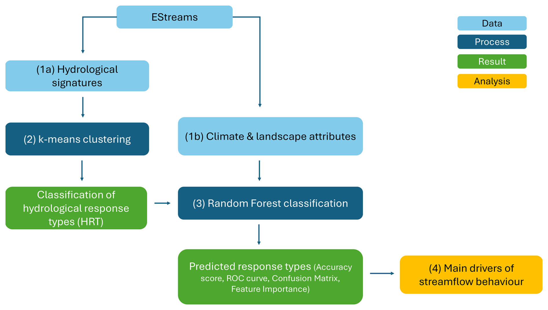
Figure 1 Workflow of the study. Streamflow time series and catchment attributes (1) were used to classify hydrological response types (HRT) to the individual catchments via k-means clustering (2) and predict HRT membership using a Random Forest classification model (3). The importance of individual attributes was quantified from the Random Forest classification model to identify the dominant controls on HRT membership and thus the main drivers of the hydrological response (4).

3.1 Signatures and attributes

The streamflow signatures and climate- and landscape attributes are compiled from the EStreams dataset (do Nascimento et al., 2024) and include long-term averages, as well as inter-annual variability around these averages (for derivation details and sources of the non-standard signatures and attributes, see Tables S1 and S2 in the Supplement). For variables that represent the intra-annual timing, the average timing signatures and attributes were calculated with circular statistics to account for the circularity of the year (Parajka et al., 2010; Blöschl et al., 2017; Berghuijs et al., 2025). Specifically, the normalised day of year, t_norm (ranging from 0 to 1) was mapped onto the unit circle using two dimensionless circular coordinates:

$$\begin{array}{}\text{(1)}& {\displaystyle }{t}_{\mathrm{SA}}=\sin \left(\mathrm{2}\mathit{\pi }{t}_{\mathrm{norm}}\right)\text{(spring–autumn axis)},\text{(2)}& {\displaystyle }{t}_{\mathrm{WS}}=\cos \left(\mathrm{2}\mathit{\pi }{t}_{\mathrm{norm}}\right)\text{(winter–summer axis)}\end{array}$$

This decomposition ensures that dates near the year boundary (e.g., 31 December and 2 January ) are represented as adjacent points on the circle, allowing for a correct computation of mean timing. The circular mean coordinates $(\stackrel{\mathrm{‾}}{t_{\mathrm{SA}}},\stackrel{\mathrm{‾}}{t_{\mathrm{WS}}})$ were then converted back to day of year using $t_{\mathrm{doy}}=(\mathrm{365.25}/\mathrm{2}\mathit{\pi })\times \mathrm{atan}\mathrm{2}(\stackrel{\mathrm{‾}}{t_{\mathrm{SA}}},\stackrel{\mathrm{‾}}{t_{\mathrm{WS}}})$, producing an unambiguous average day of the year. In this mapping, $t_{\mathrm{WS}}=+\mathrm{1}$ corresponds approximately to 1 January and $t_{\mathrm{WS}}=-\mathrm{1}$ to 1 July, while $t_{\mathrm{SA}}=+\mathrm{1}$ corresponds approximately to 1 April and $t_{\mathrm{SA}}=-\mathrm{1}$ to 1 October . For subsequent analysis with k-means clustering and Random Forest classification, the sine and cosine components $(\stackrel{\mathrm{‾}}{t_{\mathrm{SA}}},\stackrel{\mathrm{‾}}{t_{\mathrm{WS}}})$ were used directly. However, throughout the manuscript, timing is for clarity mostly reported as the reconstructed day of year t_doy (noted as t). Further details on the circular-statistics approach for computing timing signatures and related attributes are provided in Sect. S1 in the Supplement.

In a deliberate decision to preserve and use as much information as possible to characterise the hydrological response, the k-means clustering and Random Forest classification analysis were based on a comprehensive set of signatures and attributes. Note that all signatures and attributes used in the study contain independent information. Signatures and attributes that are consistently and strongly correlated with multiple other signatures and attributes were discarded after a preliminary scan. Some of the signatures and attributes retained for the analysis contain some overlapping information, but overall the level of correlation was considered low enough to be acceptable (Fig. S1), in particular as k-means clustering and Random Forest classification are rather robust in the presence of correlated variables (Breiman, 2001).

In the following sections, the hydrological signatures and climate- and landscape attributes are referred to with a capital letter followed by the variable name in subscript to clearly distinguish between the different categories, the following notation is used: hydrological signatures are denoted with an H, the climate attributes with C, the landscape attributes are categorised into vegetation and landcover denoted by V, soil with S, geology with a G, topography with a T, and the anthropogenic attributes with an A.

3.1.1 Hydrological signatures

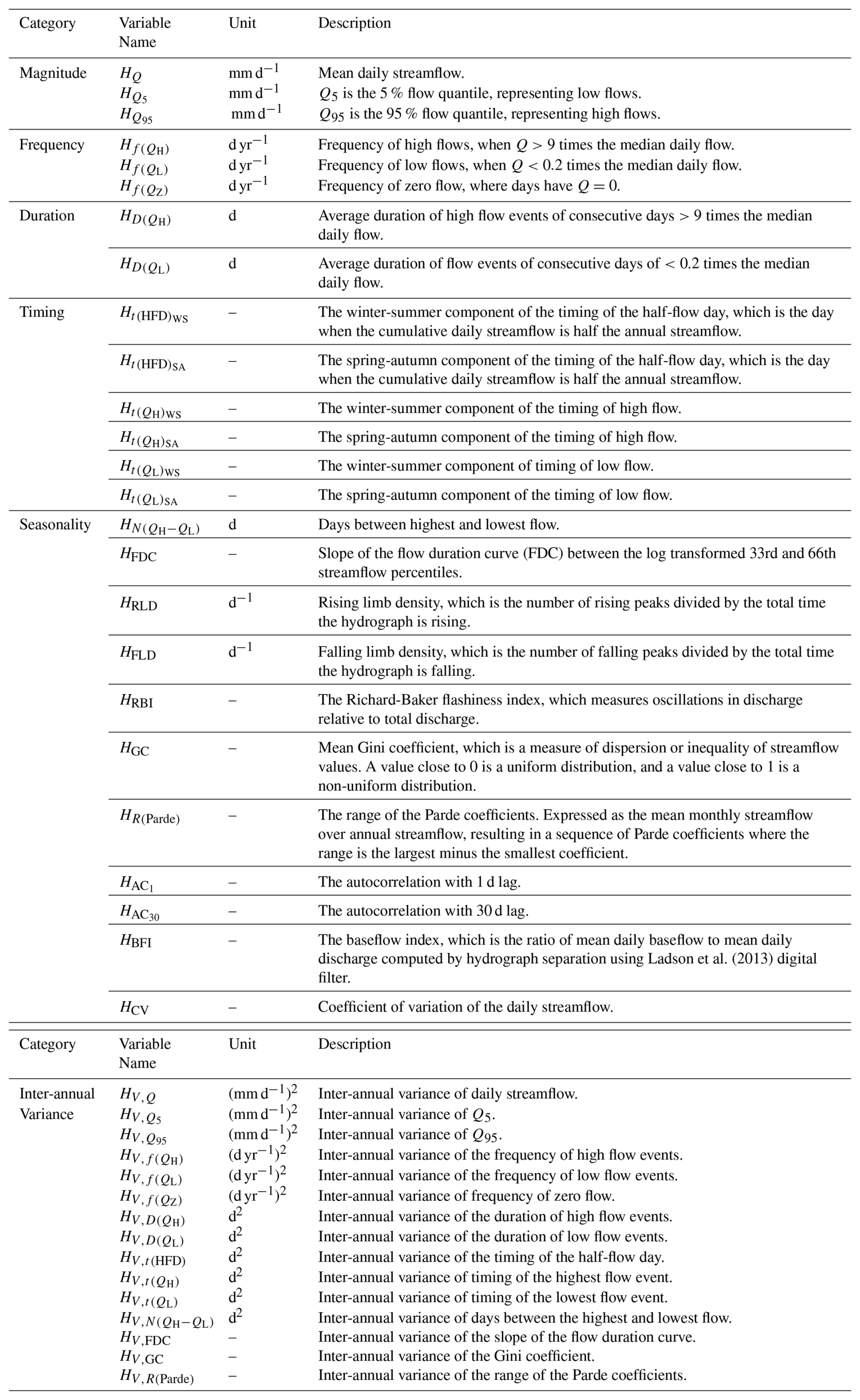
The hydrological signatures used to characterise the hydrograph included many commonly used signatures such as the long-term averages of annual mean flow (H_Q), high and low flow percentiles ($H_{Q_{\mathrm{95}}}$ and $H_{Q_{\mathrm{5}}}$), the baseflow index (H_BFI) or metrics that describe seasonality, such as the Gini coefficient (H_GC) (e.g., McMillan et al., 2017; Addor et al., 2018). Here, we define $H_{Q_{\mathrm{95}}}$ as high flows and $H_{Q_{\mathrm{5}}}$ as low flows, following the notation used in Addor et al. (2017) and do Nascimento et al. (2024). In addition, multiple signatures that characterise the average intra-annual timing of flows, such as the half-flow day (H_t(HFD)) or the day of the annual maximum ($H_{t\left(Q_{\mathrm{H}}\right)}$) and minimum flows ($H_{t\left(Q_{\mathrm{L}}\right)}$) were included in this study. The long-term averages were complemented by further signatures that quantify the inter-annual variability around these averages, such as the variances of Q (H_V,Q), the variance of high flows ($H_{V,Q_{\mathrm{95}}}$) and the variance of the half-flow day (H_V,t(HFD)). A total of 40 hydrological signatures, constructed from >90 million individual data points, were retained as sufficiently independent and used in the analysis (Table 1). To structure this high-dimensional description of the hydrological response, the signatures were loosely grouped into six categories that describe the magnitude (e.g. H_Q, $H_{Q_{\mathrm{95}}}$, $H_{Q_{\mathrm{5}}}$), the frequency (e.g. $H_{f\left(Q_{\mathrm{H}}\right)}$, $H_{f\left(Q_{\mathrm{L}}\right)}$, $H_{f\left(Q_{\mathrm{Z}}\right)}$), the duration (e.g. $H_{D\left(Q_{\mathrm{H}}\right)}$, $H_{D\left(Q_{\mathrm{L}}\right)}$), the timing (e.g. H_t(HFD), $H_{t\left(Q_{\mathrm{H}}\right)}$, $H_{t\left(Q_{\mathrm{L}}\right)}$), the seasonality (e.g. Gini coefficient H_GC and baseflow index H_BFI) and the inter-annual variability (e.g. (H_V,Q), ($H_{V,Q_{\mathrm{95}}}$), ($H_{V,f\left(Q_{\mathrm{L}}\right)}$)).To further assess the dimensionality and degree of redundancy within the selected hydrological signatures, a Principal Component Analysis (PCA) was performed on the full set of signatures to characterise the structure of variability across the components.

Ladson et al. (2013)

Table 1 Overview of the hydrological signatures derived from the EStreams dataset (do Nascimento et al., 2024). Detailed descriptions of the derivation of each signature are provided in Table S1.

By covering such a wide range and level of detail in hydrological signatures, it is expected that a relatively detailed pattern with a high number of classes of different hydrological response types can be distinguished across Europe.

3.1.2 Climate and landscape attributes

In total, 84 climate- and landscape attributes were used in the subsequent analysis. The 47 climate attributes include the long-term averages of magnitudes of hydro-climatic variables such as liquid water input ($C_{P_{\mathrm{L}}}$), i.e. rainfall plus snowmelt, temperature (C_T), potential evaporation ($C_{E_{\mathrm{P}}}$) or actual evaporation ($C_{E_{\mathrm{a}}}$), but also of derived quantities such as the aridity index $C_{\mathrm{AI}}=\frac{E_{\mathrm{P}}}{P}$ and the maximum annual water deficit C_WD as calculated from the running sum of P−E_a for each year. In addition, multiple attributes that describe aspects of timing and duration, such as the average day of the year with the highest liquid water input $C_{t\left(P_{\mathrm{L},max}\right)}$, or the duration of periods with water deficit C_D(WD), were used (Table 2). The long-term average attributes were complemented by the inter-annual variance around these averages for multiple attributes, such as the variance of liquid water input ($C_{V,P_{\mathrm{L}}}$), potential evaporation ($C_{V,E_{\mathrm{P}}}$) or the variance of the timing of the maximum annual water deficit ($C_{t\left({\mathrm{WD}}_{max}\right)}$). Note that the attributes involving snow processes were derived using a simple degree-day snow model to separate the available precipitation data into rainfall ($C_{P_{\mathrm{R}}}$), snowfall ($C_{P_{\mathrm{S}}}$), meltwater ($C_{P_{\mathrm{M}}}$) and the corresponding liquid water input $C_{P_{\mathrm{L}}}=C_{P_{\mathrm{R}}}+C_{P_{\mathrm{M}}}$ (see Sect. S4 for further information).

(Hargreaves and Samani, 1982)

Table 2 Climate- and landscape attributes derived from the EStreams dataset (do Nascimento et al., 2024). For description of derivation and original data sources, see Table S2.

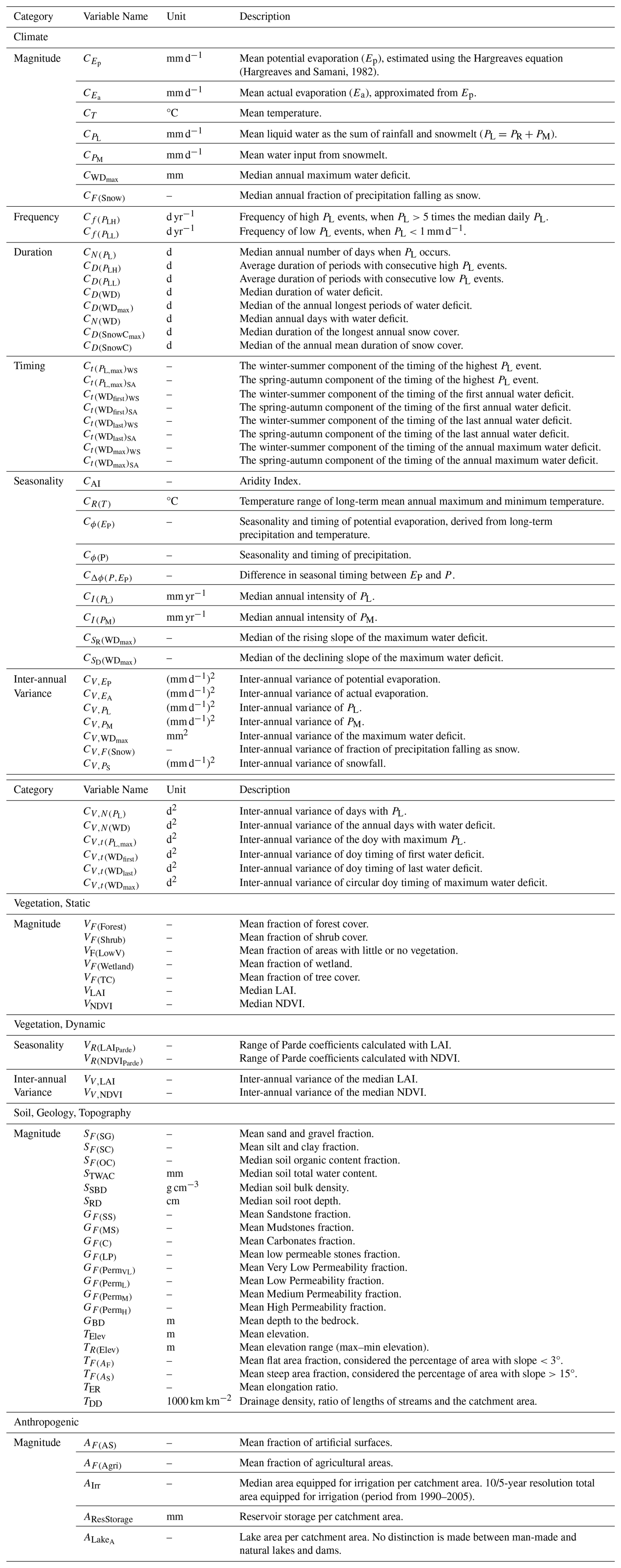
The 37 landscape attributes include subgroups of vegetation and landcover, soil, geology and topography, as well as anthropogenic attributes (Table 2). The vegetation and landcover attributes include, on the one hand, static attributes, which are either long-term averages in the case of vegetation indices such as LAI or attributes of specific years (1990, 2000, 2006, 2012, 2018) in the case of landcover from the CORINE database. On the other hand, dynamic vegetation attributes, such as the seasonality (i.e. range of the Parde coefficient) and inter-annual variances of LAI and NDVI (period from 2001–2022), were additionally distinguished as they may reflect short-term vegetation responses to hydro-climatic input.

3.2 k-means clustering

To identify hydrological similarity between our catchments in the form of multiple HRTs, k-means clustering, a technique frequently used in comparable studies, was applied (Sawicz et al., 2011; Kuentz et al., 2017; Brunner et al., 2020; Almagro et al., 2024). k-means clustering groups catchments by dividing the dataset into a predefined number of clusters (here: HRTs), each represented by a centroid. The algorithm iteratively assigns each catchment to the nearest centroid based on Euclidean distance, and then updates the centroid positions to minimise the within-cluster sum of squared distances. Because the number of clusters k must be specified beforehand, it is necessary to evaluate different choices of k to identify a solution that balances cluster compactness and interpretability. Two common evaluation metrics are the Elbow Method and the Silhouette Score. The Elbow Method assesses how the total within-cluster variance decreases with increasing k, with a breakpoint, i.e. an “elbow” indicating a point beyond which additional clusters do not provide substantial improvements. It is reported as inertia, which is the sum of the squared distances to the closest cluster centroid, for each catchment. The Silhouette Score, on the other hand, quantifies how similar each catchment is to its assigned cluster compared to other clusters, with higher values reflecting better-defined and more distinct clusters. The k-means clustering algorithm was run for a range of k from 2 to 20. The most suitable number of clusters and thus HRTs was determined using the Elbow Method and Silhouette Score metrics. To ensure that all hydrological signatures contributed equally to the clustering, the variables were normalised using min–max scaling to account for their different units and magnitudes. The k-means clustering resulted in a set of k hydrologically similar groups (HRTs), with each catchment assigned to one of these HRT classes (labelled 1 to k). These HRT class labels were subsequently used as the target variable in the Random Forest classification model.

3.3 Random Forest classification

The Random Forest classification model, implemented with the scikit-learn Python library, was used here with the climate- and landscape attributes as input features to predict the membership of each catchment to one of the classes of hydrological response types (HRT) (Sect. 4.2) in a supervised multiclass classification problem. The idea behind this is that each HRT class represents a unique combination of hydrological characteristics as defined by the hydrological signatures. By predicting catchment membership to the class of HRT from climate- and landscape attributes, it can then be analysed to which extent hydrological classes can be predicted based on landscape and climate, as well as which climate- and landscape attributes are more relevant for shaping hydrological response pattern. While Random Forest regression models have been successfully used to predict individual hydrological signatures (e.g., Addor et al., 2018; Almagro et al., 2024), predicting membership to a HRT class, representing a multi-dimensional composite of hydrological signatures, provides a complementary perspective that may help reveal the drivers of overall hydrological behaviour and its spatial variability.

As the choices made in the modelling process can substantially affect the results and interpretation thereof, a stepwise approach with many alternative model set-ups was applied here. In a first step, each model was tuned through iterative adjustment of hyperparameters in a Monte Carlo sampling strategy with 5000 realisations. Each realisation was evaluated based on its accuracy, i.e. the fraction of correctly classified catchments over the total sample (Acc = true positives/total sample) for both training and validation. From the set of all realisations, a solution was chosen that balances a good training (Acc_t≥0.6) with a robust validation performance Acc_val ($\mathrm{\Delta }{\mathrm{Acc}}_{\mathrm{t}}-{\mathrm{Acc}}_{\mathrm{val}}\le \mathrm{0.1}$) to limit overfitting (for the retained solution's model parameter set see Sect. S7). In the second step, the retained solution was used to further train and evaluate the model using a 10-fold cross-validation, with 90 % of the data, i.e. catchments in a HRT, used for training and 10 % for testing in each fold. Due to the unequal number of catchments in the individual HRTs, the HRTs were weighted according to their respective number of catchments in the model. After that initial model set-up that predicted membership to 10 individual HRT classes, the same sequence of steps was repeated using 6, 7, 8 and 9 HRT classes, respectively, to analyse the sensitivity of the model and to assess how well the HRTs are defined.

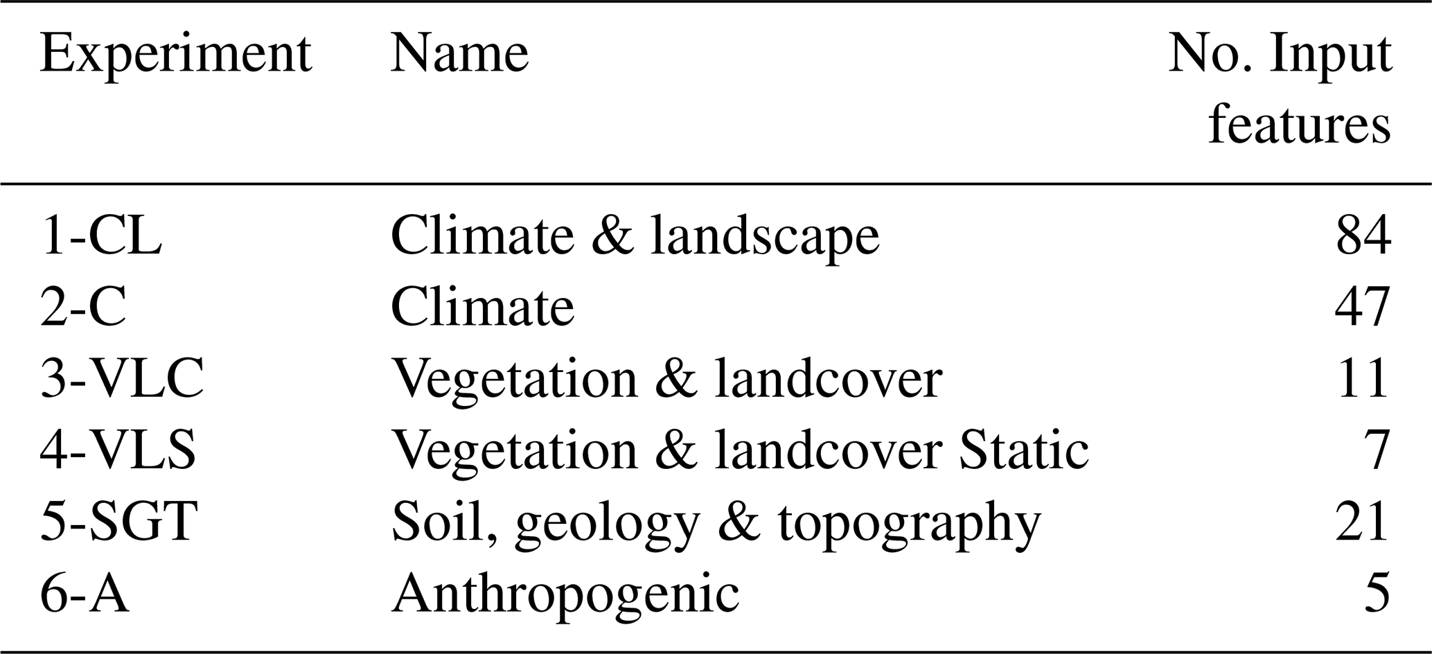
To evaluate in a last step, the relative influences of climate and landscape on hydrological behaviour, five experiments were conducted in addition to the initial experiment (1-CL). In these experiments, the Random Forest classification model was trained and tested using only climate- or different landscape-attributes (Table 3). In Experiment 2-C, exclusively the 47 climate attributes were used for model training and testing, while Experiment 3-VLC used the 11 vegetation and landcover attributes. As some of the vegetation signatures may directly reflect short-term climatic variability, Experiment 4-VLS used only the 7 static vegetation and landcover attributes. Experiment 5-SGT included the 21 signatures related to soil, geology and topography, and Experiment 6-A used the 5 anthropogenic attributes.

Table 3 Random Forest classification experiments.

For the analysis of the climate- and landscape-controls on the HRTs in the six experiments, model performances are reported as averages over the cross-validation folds. Besides the accuracy Acc, model performance of each experiment was evaluated using receiver operating characteristic curves (ROC curves), the area-under-the-curve metric (A_UC) and the confusion matrix for a more nuanced picture of the true positive, false positive and false negative rates of the classification. The ROC curve illustrates the model performance across varying classification thresholds by plotting the true positive rate against the false positive rate, demonstrating the relative trade-off between the correctly and incorrectly classified instances. The classification threshold determines how predicted probabilities are turned into class labels. For example, if the threshold is 0.5, a catchment with a predicted probability of ≥0.5 of belonging to class A, will be classified as A. Changing this threshold shifts the balance between correct and incorrect classifications, and the average of all the different true and false positive rates makes up the ROC curve. An overall robust and well-performing model approaches the upper left corner (high true positive rate R_TP and low false positive rate R_FP), reaching high A_UC values, while poorer model performance with lower A_UC is reflected by curves closer to the diagonal, which represents random guessing.

However, dealing with a multiclass prediction, the ROC curves and A_UC are averaged across all HRT classes and folds, and therefore only provide partial information on the model performance. To assess the final classification outcomes, confusion matrices were used. These compare the true HRT class to the predicted HRT class, with correct predictions, i.e. true positive rates, for each HRT plotting along the diagonal. Each row represents the true HRT, and each column the predicted HRT. Off-diagonal rows therefore, indicate the false negative rates, while off-diagonal columns show the false positive rates. Together, this provides insights into which HRTs are more robustly predicted than others and which HRTs are more susceptible to misclassifications.

For each experiment, permutation feature importance scores from the associated Random Forest classification model were used to evaluate the relative contributions of the climate- and landscape attributes to the model performance. Feature importance reveals to which extent a feature (here: climate- or landscape attribute) influences the classification outcome. It is quantified for each feature as the decrease in predicted accuracy when this specific feature is removed from the model. To ensure that feature importance scores were robust, it was calculated 10 times for each of the folds. The reported feature importance is the average of the 10 calculations across all folds.

4 Results

4.1 Classes of hydrological response types across Europe

Preliminary k-means clustering runs with k ranging from 2 to 20 (representing predefined numbers of HRTs based on the available hydrological signatures) did not yield a clear or unambiguous optimal number of HRTs. While the Inertia metric of the Elbow Method indicates no apparent break but rather a smooth decline with an increasing number of HRTs (Fig. 2a), the Silhouette Score metric suggests a major break at k=4 and another minor break at 12 HRTs (Fig. 2b). The generally low values of the Silhouette Score, i.e. <0.25, further indicate that it is unlikely that the number of well-defined HRTs exceeds that range.

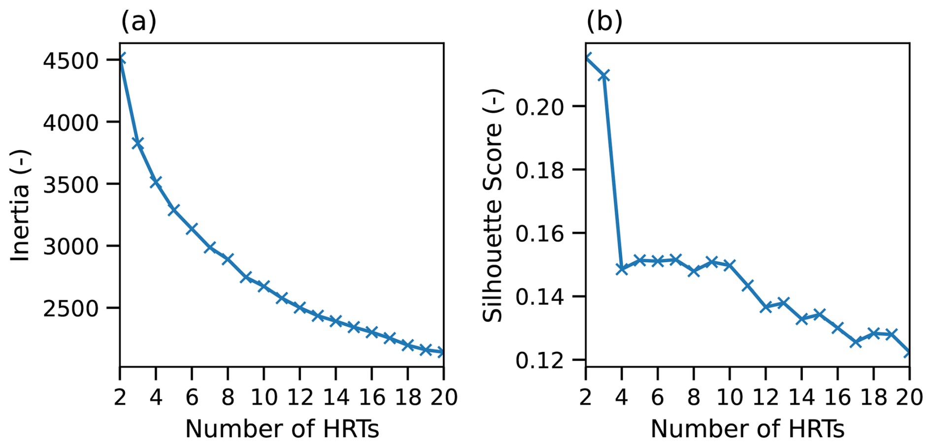
Figure 2 Assessment of cluster robustness using k-means clustering. (a) Elbow Method results for k=2–20 HRTs, used to evaluate the optimal number of hydrological response types. (b) Silhouette Scores for the same range of HRTs, providing an additional metric of cluster cohesion and separation.

As a balanced choice to allow for some detail while not inflating the number of HRTs warranted by the data, the results are thus hereafter reported with a focus on 10 HRTs. However, to test the significance of the choice of HRTs numbers on the results, the results of k-means clustering with 6, 7, 8, and 9 HRTs were compared to the 10 HRTs, but no substantial difference was found between the different HRT numbers, see Fig. S3.

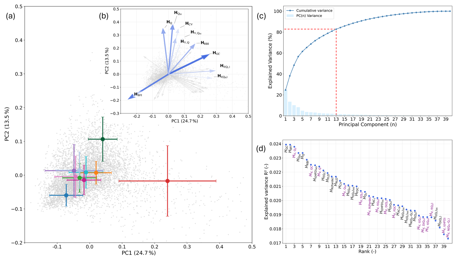
Figure 3 Principal Component Analysis (PCA) of the 40 hydrological signatures across the HRTs. (a) Explained variance of PC1 (24.7 %) and PC2 (13.5 %) for each catchment (grey), with HRT means and standard deviations shown in their respective colour. (b) Loadings of the hydrological signatures, shown for PC1 and PC2. Arrow thickness and colour intensity reflect each signature's ranked explained variance based on the first 13 PCs (see panel d), accounting for just above 80 % of the cumulative explained variance. Thicker and more intense coloured arrows indicate more informative signatures. (c) Cumulative explained variance across all principal components. The explained variance of the first 13 PCs is highlighted by the red dashed lines. (d) Ranked explained variance of the first 13 PCs, which together account for approximately 80 % of the total variance. Signatures related to variance are highlighted in purple.

Overall, Fig. 2 suggests that there is little evidence that the set of 40 hydrological signatures used for this analysis contains sufficient information to robustly distinguish more than 10 different types of HRTs for the 7175 study catchments across Europe. The results of a Principal Component Analysis of the signatures further support this interpretation. Indeed, as shown in Fig. 3a, the first two principal components (PC) account for merely ∼38 % of the variance in the signatures, and at least 19 principal components are required to explain >90 % of the variance (Fig. 3c). This suggests that the signatures cannot be effectively compressed due to a low level of redundancy in their respective information contents and suggesting that signatures of individual catchments exhibit substantial scatter but not in a systematic enough manner. The latter implies that no detailed pattern of similarity that would go beyond ∼10 HRTs could here be identified based on k-means clustering. As a further consequence, the within-HRT variability of individual signatures can be substantial. Showing the distributions of several selected signatures, Fig. 4 illustrates that some signatures, such as the baseflow index H_BFI (Fig. 4e), the Gini coefficient H_GC (Fig. 4f) or the flashiness index H_RBI (Fig. 4i), exhibit a clear contrast across the HRTs and limited within-HRT variability which can also be seen by the standard deviations of the signatures around the normalised means of the individual HRTs in Fig. 5. In contrast, many other signatures such as the days between highest and lowest flow $H_{N(Q_{\mathrm{H}}-Q_{\mathrm{L}})}$ (Fig. 4j) or the autocorrelation coefficient $H_{{\mathrm{AC}}_{\mathrm{30}}}$ (Fig. 4g) are characterised by substantial within-HRT variability, lower across-HRT contrast and thus little discriminatory power which can be seen by the limited differences between the standard deviations of these signatures across the HRTs in Fig. 5. Note that the distributions of all hydrological signatures in the individual HRTs is provided in Fig. S2.

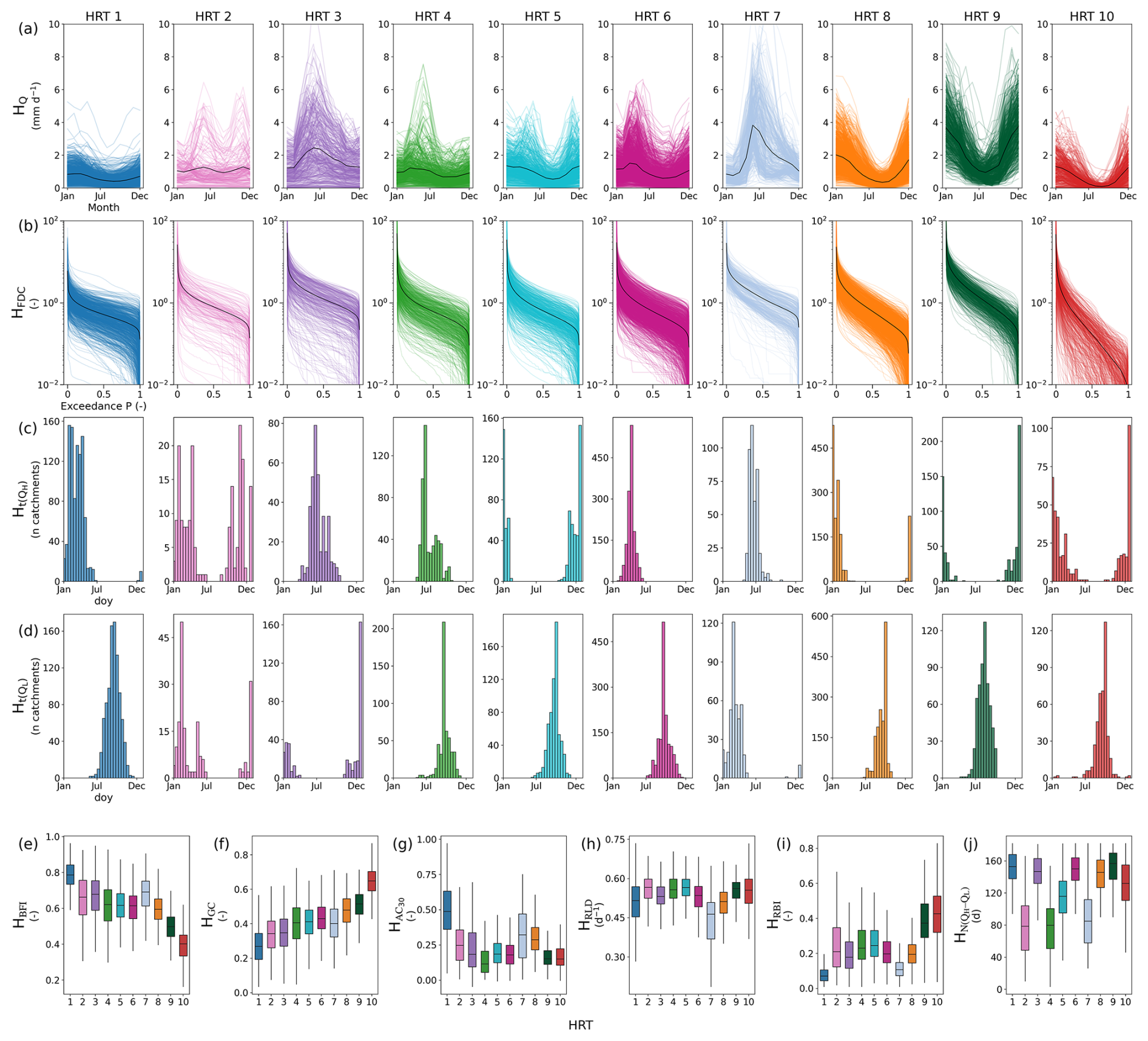
Figure 4 Visualisation of 10 out of the 40 hydrological signatures across hydrological response types (HRTs), the remaining 30 signatures can be seen in Fig. S2. Panels (a)–(d) show four selected signatures for each HRT (one row per signature, one column per HRT), (a) streamflow (H_Q), (b) flow duration curves (H_FDC), (c) high flow timing ($H_{t\left(Q_{\mathrm{H}}\right)}$) and (d) low flow timing ($H_{t\left(Q_{\mathrm{L}}\right)}$), highlighting within- and between-cluster variability. In panels (a) and (b), the black line indicates the mean value of mean discharge (Q) and mean flow duration curve (FDC), respectively. Panels (e)–(j) display boxplots of six additional hydrological signatures, (e) baseflow index (H_BFI), (f) Gini coefficient (H_GC), (g) autocorrelation ($H_{{\mathrm{AC}}_{\mathrm{30}}}$), (h) rising limb density (H_RLD), (i) flashiness index (H_RBI) and (j) days between highest and lowest flow ($H_{N(Q_{\mathrm{H}}-Q_{\mathrm{L}})}$), summarising their distribution across HRTs.

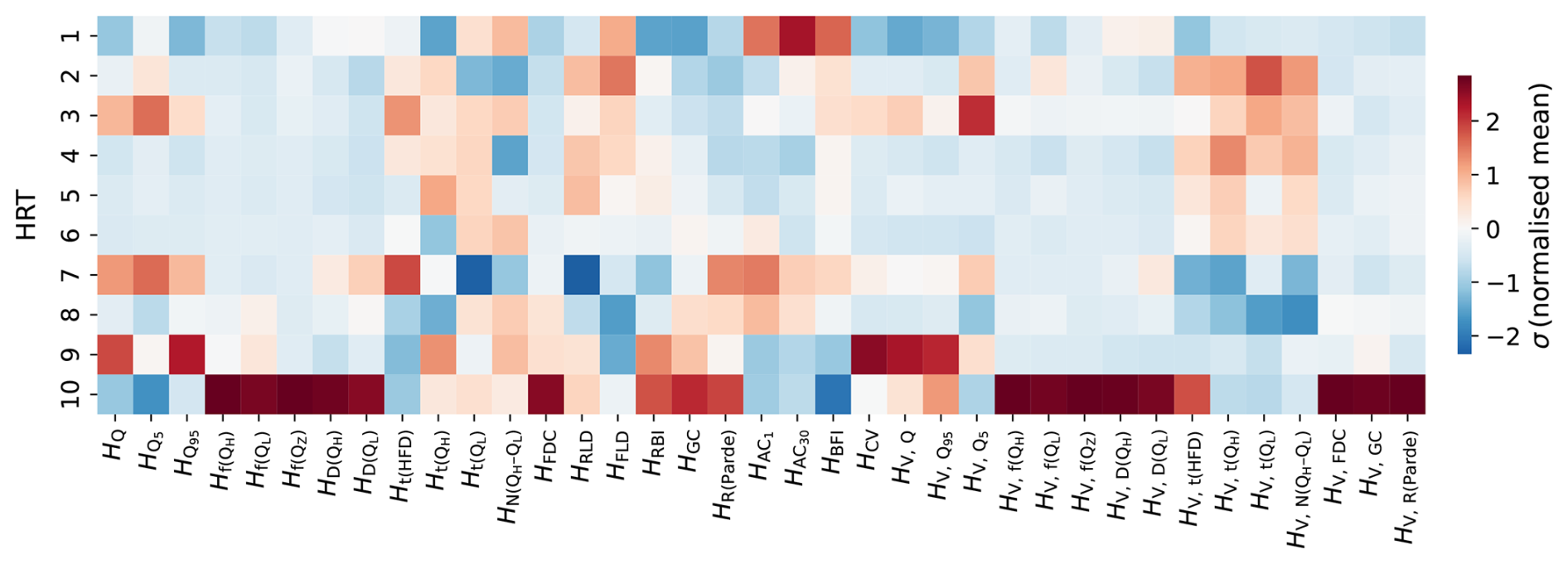
Figure 5 Standard deviation of the normalised mean for each hydrological signature shown for each HRT. Positive deviations are shown in red and negative deviations in blue, with colour intensity indicating the magnitude of the deviation.

The most informative hydrological signatures, ranked by their cumulative variance across the first 13 PCs (∼80 % of variance explained) as shown in Fig. 3b and d, included the Gini coefficient H_GC as metric of flow seasonality (1st rank), the baseflow index H_BFI (2nd) as metric of flow stability, the mean flow H_Q (5th) as metric of overall flow magnitude but also descriptors of inter-annual variance, such as $H_{V,Q_{\mathrm{5}}}$ as metric of variance of low-flow magnitude (3rd), and the variance of the Gini coefficient H_V,GC, as metric of inter-annual differences in flow seasonality (7th). The picture that emerges illustrates that while a few signatures of inter-annual variability are among the top-ranked ones, the majority of them, i.e. 10 out of 15, ranks in the bottom half of all signatures. HRTs are thus dominantly defined by signatures of averages, in particular flow seasonality, stability and magnitude (Fig. 3d).

Building on these defining signatures, the 10 HRTs exhibit a wide range of hydrological behaviours, with varying degrees of distinctness (Fig. 4, Table 4).

Table 4 Overview of the 10 hydrological response type classes (HRTs). The labels focus on hydrological signatures H_Q and $H_{t\left(Q_{\mathrm{H}}\right)}$ (Fig. 4a and c). The characteristics focus further on those most distinct within each HRT, like the contribution of baseflow, timing of highest and low flows and flashiness, while geography can be visually checked in Fig. 6.

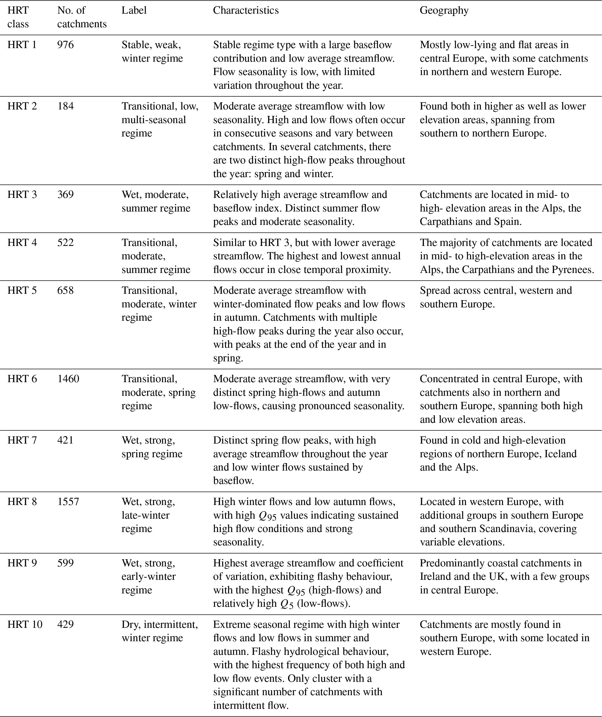
For example, HRTs 1 (stable, weak, winter regime), 7 (wet, strong, spring regime), 8 (wet, strong, late-winter regime), 9 (wet, strong, early-winter regime) and 10 (dry, intermittent, winter regime) are readily distinguishable (Fig. 4a–d) due to their stable, strong or extreme flow-regime characteristics. HRT 1 represents a highly stable regime with low mean flows, high baseflow (H_BFI) contributions and the lowest flashiness index (H_RBI) (Fig. 4a, e, i). In contrast, HRT 10 shows an extreme regime characterised by very steep flow duration curves (H_FDC) and strong seasonality as illustrated by the highest Gini coefficients (H_GC) (Fig. 4b, f), while HRTs 7–9 exhibit pronounced seasonal peaks and lows and highly consistent timing of high flows ($H_{t\left(Q_{\mathrm{H}}\right)}$) (Fig. 4a, c, d). In contrast, less distinct HRTs, such as HRT 2 (transitional, low, multi-seasonal regime), show a wide spread in the timing of high and low flows ($H_{t\left(Q_{\mathrm{H}}\right)}$, $H_{t\left(Q_{\mathrm{L}}\right)}$) and in the slopes of the flow duration curves (H_FDC), whereas HRT 5 (transitional, moderate, winter regime) remains close to the overall average for most signatures (Figs. 4, 5). However, the within-HRT variability is not uniform, each HRT shows limited variability in some signatures and substantial spread in others. For example, HRT 1 shows low variability in the baseflow (H_BFI) and flashiness (H_RBI) indices but high variability in autocorrelation($H_{{\mathrm{AC}}_{\mathrm{30}}}$) and rising limb density (H_RLD). Similarly, HRT 7 has tightly grouped flashiness (H_RBI) and high-flow timing ($H_{t\left(Q_{\mathrm{H}}\right)}$), but a wide spread in rising limb density (H_RLD) and the days between high and low flows ($H_{N(Q_{\mathrm{H}}-Q_{\mathrm{L}})}$). Less distinct classes, such as HRT 2, show a similar variation in signature values, with relatively low variability in rising limb density (H_RLD) but high variability in baseflow (H_BFI) and flashiness (H_RBI) indices and the timing of flows ($H_{t\left(Q_{\mathrm{H}}\right)}$, $H_{t\left(Q_{\mathrm{L}}\right)}$) (Fig. 4c, d, e, i). These heterogeneous patterns illustrate why detailed descriptions of the HRTs beyond the major contrasts remain challenging.

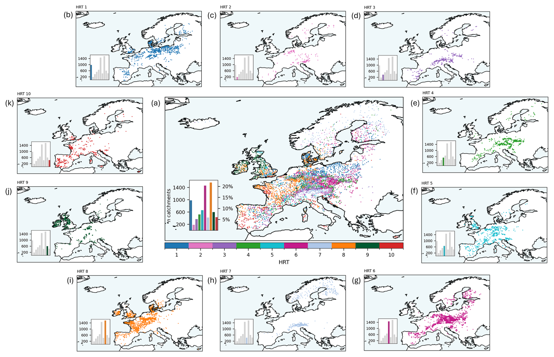
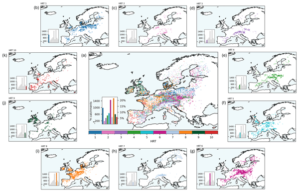
Figure 6 Classification of 7175 catchments into 10 HRT based on 40 hydrological signatures. The HRTs are ordered by increasing slope of the flow duration curves. Panel (a) presents all HRTs together, panels (b) to (k) show the spatial distribution of each HRT individually.

Despite the difference in within-HRT hydrological signature variation, broad hydrological patterns emerge across the HRTs and form the basis for their classification into flow-regime types (Table 4). Key characteristics, reflecting the dominant signatures from PCA analysis (Fig. 3d), include the magnitude of average discharge, the strength and shape of the seasonal cycle, and the predominant season of high flows. Using these criteria, the HRTs range from stable to transitional, wet, and dry regimes, and from weakly seasonal to strongly seasonal systems with winter-, spring-, summer-, or multi-seasonal peak-flow timing. The geographical distribution of the HRTs as shown in Fig. 6, reflects some of these large-scale hydrological differences but does not show consistent spatial clustering. Certain HRTs are geographically concentrated: for example, HRT 7 (wet, strong, spring regime) is largely confined to the Alps, northern Scandinavia and Iceland (Fig. 6h), while HRT 9 (wet, strong, early-winter regime) is mainly located in the UK and Ireland (Fig. 6j). Other well-defined classes, such as HRT 10 (dry, intermittent, winter regime) and HRT 8 (wet, strong, late-winter regime), are more widely distributed across Europe. Likewise, HRT 1 (stable, weak, winter regime) and HRT 6 (transitional, moderate, spring regime) span a broad latitudinal gradient from southern Spain to Finland, while HRT 3 (wet, moderate, summer regime) and HRT 4 (transitional, moderate, summer regime) are clustered in transitional regions between high and low elevations. Thus, spatial proximity may explain some, but far from all patterns in the geographical distribution of HRTs.

4.2 Prediction of HRTs by climate- and landscape attributes and drivers of streamflow behaviour

The initial hyperparameter tuning approach for model selection, based on 10 classes of HRTs and all 84 climate- and landscape attributes as input features of the Random Forest classification model to predict membership of catchments to individual HRTs, resulted in training accuracies Acc_t∼0.45–1 (Fig. S4a). In contrast, the validation accuracy Acc_val remains <0.70 for all realisations. These overall reductions of accuracies between calibration and validation indicate substantial model overfitting, and thus limited predictive power as Acc_t increases. As expected, validation accuracies increase for model set-ups based on a lower number of HRTs (k=6–9), as shown in Fig. S4b–e. However, with Acc_val not exceeding 0.7 for any of the set-ups, the improvements are very minor, while the overall pattern remains unchanged. The opposite, with partly substantial declines in predictive power, was observed with model set-ups using higher numbers of HRTs (not shown). To thus preserve both, at least moderate levels of detail in the distinction of HRTs as well as at least moderate levels of model predictive power, 10 HRTs were eventually used as a balanced choice for the subsequent analysis. More specifically, the hyperparameter set resulting in Acc_t=0.70 and Acc_val=0.60 for these initial runs (Fig. S4a) was selected for further analysis.

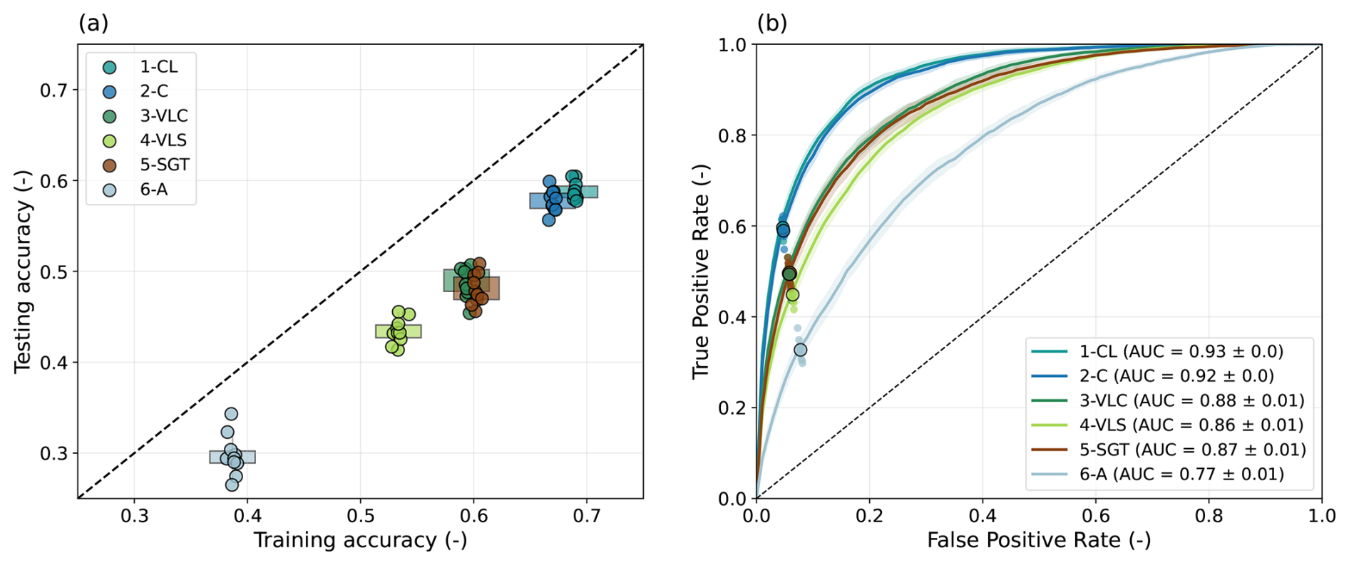
Figure 7 (a) Testing versus training accuracy for each experiment. Each circle represents one of the 10 cross-validation folds. The axes are extended slightly beyond the data range to show the 1 : 1 reference line. Boxplots beneath the points summarise the distribution of testing accuracies across the 10-fold cross-validation for each experiment. (b) The averaged ROC curves for each experiment are displayed, computed over the 10 cross-validation folds. For each fold, the true positive rate (R_TP) and false positive rate (R_FP) at the actual classification threshold are shown as small dots. The larger dot represents the average R_TP and R_FP across all folds, corresponding to the aggregated performance reported in the confusion matrices.

The first of the six full experiments, predicting membership of individual catchments to the 10 different HRTs based on the complete set of 84 climate- and landscape attributes, i.e. 1-CL, resulted in rather stable results across the 10 cross-validation folds, with Acc_t=0.68–0.69 and Acc_test=0.58–0.60 (Figs. 7a and S5). A more nuanced analysis of the results reveals that, at the chosen classification threshold, the true positive rates, i.e. the fraction of catchments whose membership to a specific HRT is correctly predicted, reaches with R_TP=0.57–0.61 comparable values across all 10 folds as illustrated by the individual dots in Fig. 7b. It also illustrates that the false positive rates, i.e. the fraction of catchments with a specific HRTs whose membership to other HRTs is incorrectly predicted, remains very low with R_FP=0.04–0.05. These values describe the model's performance when turning predicted probabilities into hard class labels, and are also reflected in the confusion matrices (Fig. 8). Independently of this threshold, the ROC analysis yields an A_UC=0.93, indicating that the combined climate- and landscape attributes used in the 1-CL experiment have predictive power that is in any case substantially higher than a random guess, represented by the 1 : 1 line in Fig. 7b and the associated A_UC=0.5.

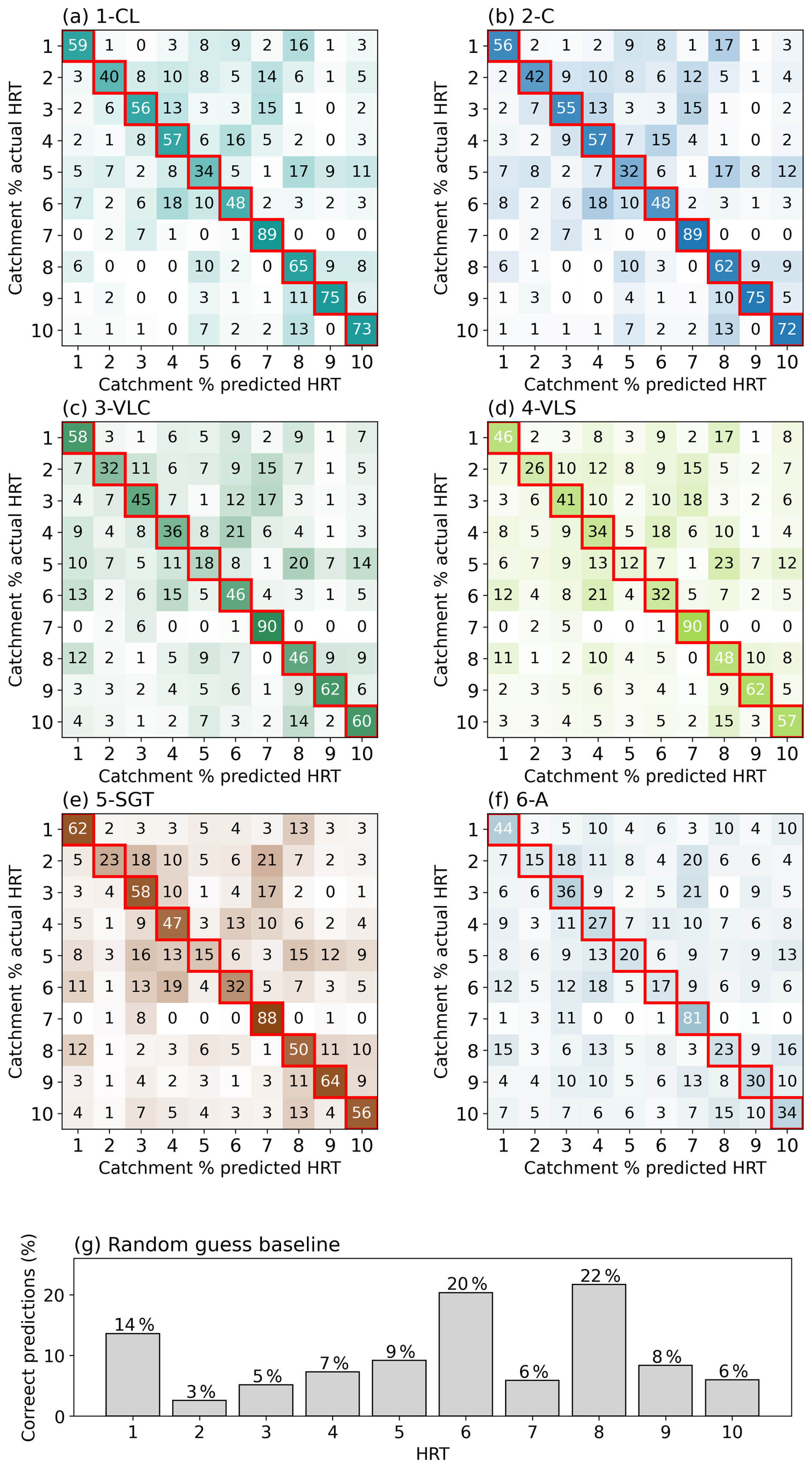
Figure 8 Confusion matrices for each hydrological response type (HRT), normalised by row (i.e., by true HRT). The diagonal elements show the percentage of catchments correctly predicted as their true HRT. Off-diagonal elements in each row represent the percentage of that HRT misclassified as other HRTs (false negatives), while off-diagonal elements in each column indicate false positives. All values are rounded to whole percentages; therefore, individual rows may not sum to exactly 100 %. For example, panel (a) shows the confusion matrix for experiment 1-CL: the first cell in row 1 (row 1, column 1) gives the percentage of HRT 1 correctly predicted as HRT 1, whereas the entry in row 1, column 2 indicates the proportion of HRT 1 predicted as HRT 2. Similarly, the value in row 2, column 1 represents the percentage of HRT 2 incorrectly predicted as HRT 1. (g) Baseline scenario showing the percentage of catchments expected in each HRT class under random guessing, based on the class distribution.

A further stratification of the results exposes pronounced differences between the individual 10 HRTs. Membership to some HRTs, such as HRTs 7 (wet, strong, spring regime) and 9 (wet, strong, early-winter regime), is with Acc_test of up to 0.89 and A_UC of up to 0.99 very well predicted (Figs. 8a and S5). These well-predicted HRTs are generally well defined by several hydrological signatures that are distinct to those of other HRTs (Figs. 4 and S5). While HRT 7 is, for example, characterised by elevated flow magnitudes, in particular H_Q and $H_{Q_{\mathrm{5}}}$, as well as markedly different timing characteristics, including the latest half-flow day H_t(HFD) and the earliest low flows $H_{t\left(Q_{\mathrm{L}}\right)}$, HRT 9 equally stands out with high H_Q, but also exhibits the highest $H_{Q_{\mathrm{95}}}$, the largest flow variability H_CV and the earliest half-flow day H_t(HFD) (Fig. S2). This is contrasted by membership to other HRTs that are less well predicted. This is in particular the case for HRT 5 (transitional, moderate, winter regime) with Acc_test=0.34 (Fig. 8a) and A_UC=0.83 (Fig. S6). As a transitional HRT, none of its hydrological signatures is clearly discernible from the other HRTs, making an effective discrimination difficult (Figs. 4 and S6).

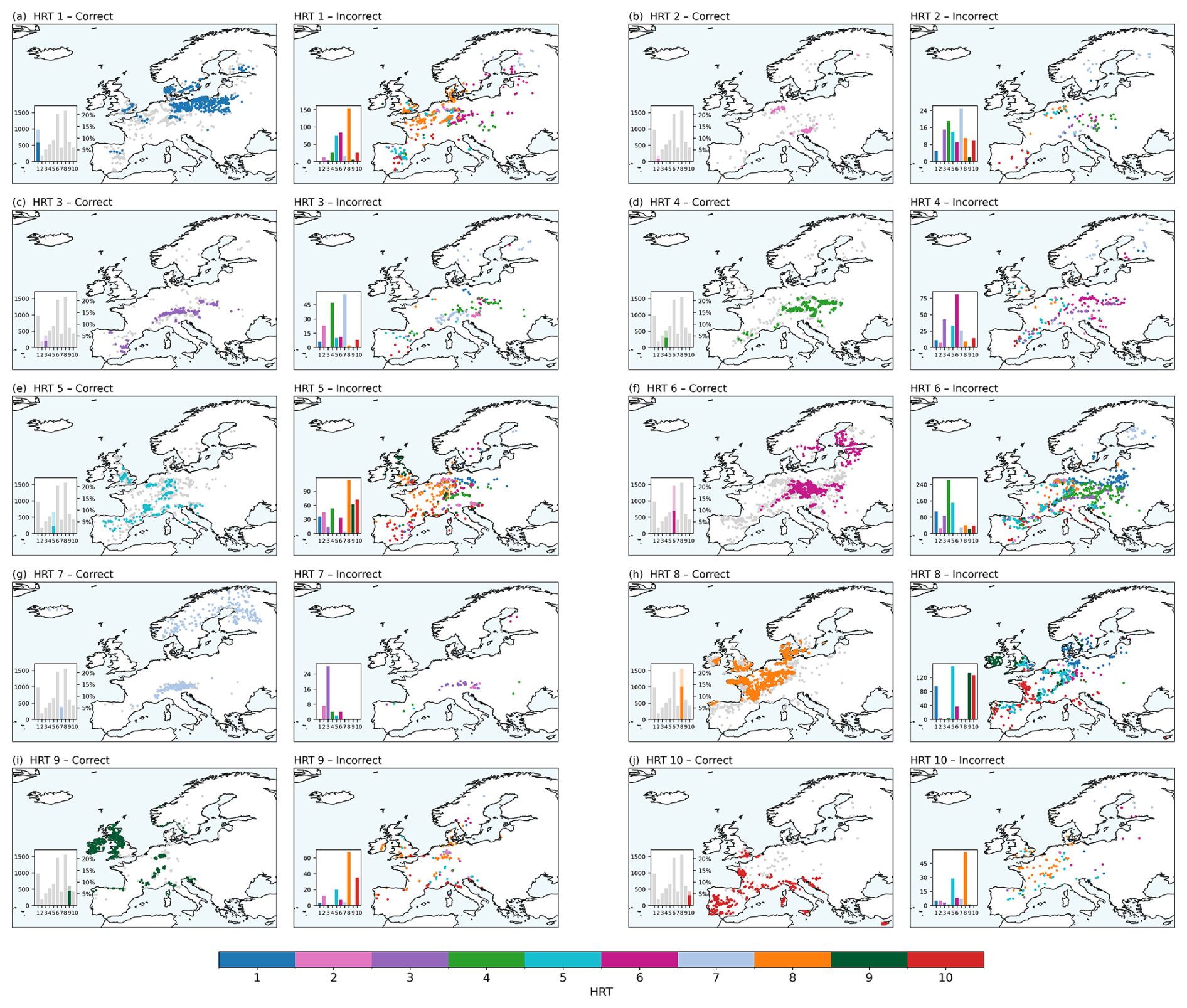
Figure 9 Maps showing correct and incorrect classification results for experiment 1-CL. In the “correct” panels, only correctly classified catchments are shown in their HRT colours, while incorrectly classified catchments appear in grey. In the “incorrect” panels, only the misclassified catchments are displayed and coloured according to their true HRT, allowing visual assessment of which clusters are most frequently misclassified.

From a spatial perspective, no clear pattern emerges in the correctly predicted HRTs (Fig. 9). However, some regions show an overrepresentation of misclassifications, notably northern Spain, the Paris Basin, South-East England, and southern Poland (Fig. 9). While HRT 10 (dry, intermittent, winter regime) is predicted fairly homogeneously across its domain (Fig. 9j), the misclassified catchments span nearly all other HRTs, with the largest share belonging to HRT 8 (wet, strong, late-winter regime). Other well-predicted classes include HRTs 7 (wet, strong, spring regime), 8, and 9 (wet, strong, early-winter regime), with HRTs 7 and 9 being the most spatially homogeneous. These HRTs occupy relatively compact hydro-climatic domains, in contrast to HRT 8, which is generally well predicted but has misclassifications distributed widely across Europe (Fig. 9g, h, i).

HRTs 2 (transitional, low, multi-seasonal regime), 5 (transitional, moderate, winter regime), and 6 (transitional, moderate, spring regime) display more spatially variable predictive performance (Fig. 9b, e, f). For HRT 2 and HRT 6, correctly classified catchments occur in dense clusters, whereas the misclassified ones are scattered across Europe. In contrast, both correct and incorrect predictions of HRT 5 are widespread. The most frequent confusions are HRT 2 being misclassified as HRT 7 (wet, strong, spring regime), HRT 5 as HRT 8 (wet, strong, late-winter regime), and HRT 6 as HRT 4 (transitional, moderate, summer regime), consistently across all experiments (Figs. 9b, e, f and S7–S11). HRT 5 and HRT 8 share similarities in timing (Fig. 4c, d), but otherwise show limited resemblance (Fig. 5). HRT 6 and HRT 4 also overlap in the timing of their high and low flows (Fig. 4c, d) and exhibit similar seasonal patterns (Fig. 4a). In contrast, a comparison of signatures between HRT 2 and HRT 7 (Fig. 5) reveals no striking similarities, suggesting that their mutual misclassification may result from similarities in climatic or landscape controls rather than hydrological behaviour alone.

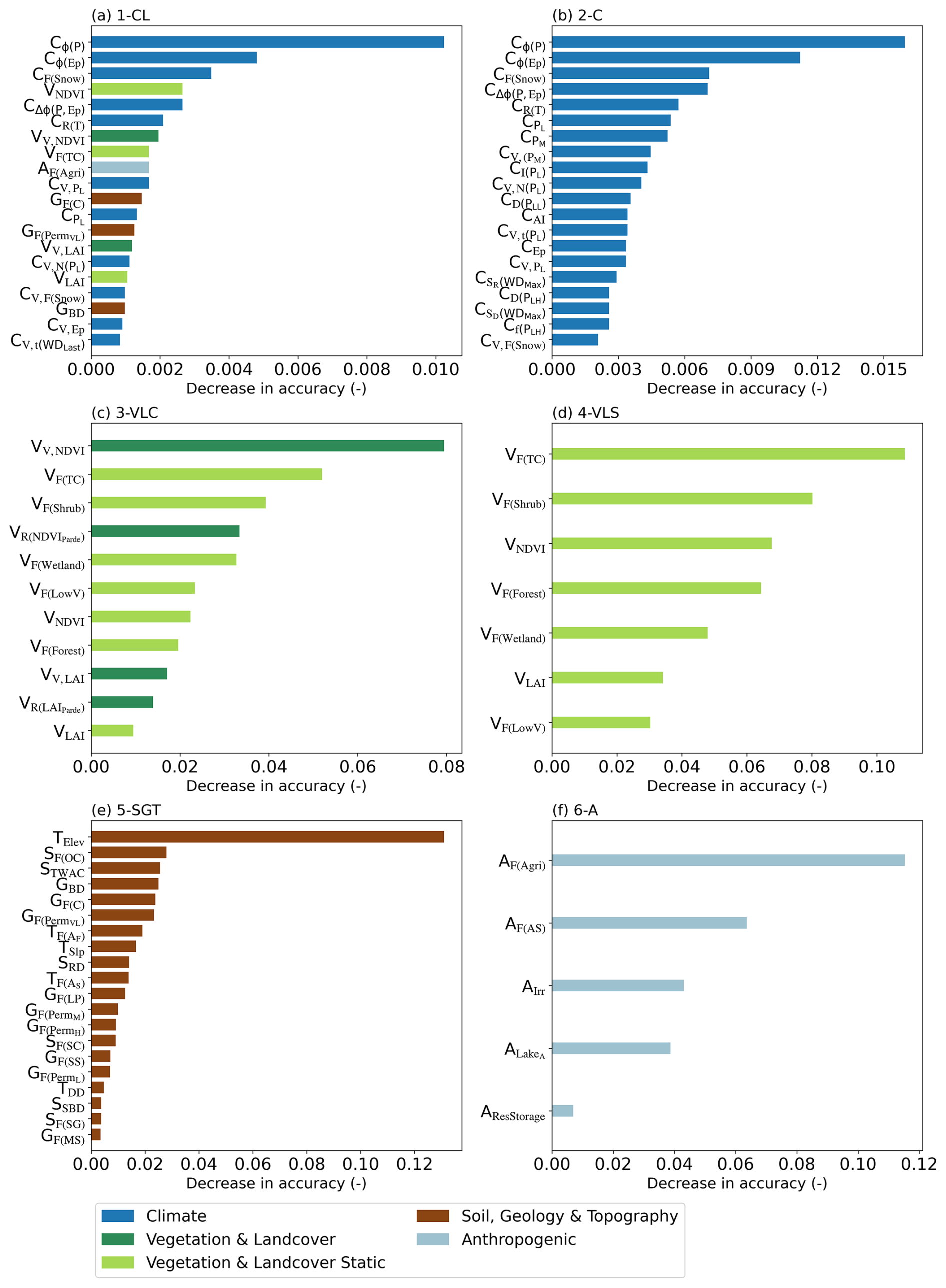
Figure 10 Median feature importance across the 10-fold cross-validation for all six experiments. Features are ranked by importance (y-axis), which is dictated by the decrease in model accuracy (Acc_test) by removing the corresponding attribute (x-axis). Panels (a), (b) and (e) display only the 20 most important features. Feature importance values are not directly comparable across experiments because they depend on the model type and the number and composition of input features; experiments with fewer predictors typically yield higher importance values per feature.

The relative roles of the individual climate- and landscape attributes as drivers of streamflow behaviour were then analysed by comparing their feature importance (Fig. 10). Overall, the seasonality of precipitation C_ϕ(P) (1st rank), the seasonality of potential evaporation $C_{\mathit{\varphi }\left(E_{\mathrm{P}}\right)}$ (2nd) as well as the fraction of precipitation falling as snow C_F(Snow) (3rd) emerge as the strongest predictors of membership to classes of HRTs and thus as most dominant controls on streamflow behaviour (Fig. 10a). Next to these three climate attributes, almost half of the top 20 ranking predictors are landscape attributes. Most notably, several descriptors of vegetation attributes such as the average NDVI V_NDVI (4th), its inter-annual variance V_V,NDVI (7th) or average tree cover fraction V_F(TC) (8th) stand out, while the fraction of carbonate rocks G_F(C) (11th) is the highest-ranking attribute from the soil, geology and topography group. In addition, the fraction of agricultural areas A_F(Agri) (9th) appears as most relevant from the group of anthropogenic attributes.

In the second experiment 2-C, predicting membership to the 10 HRTs based exclusively on the reduced set of 47 climate attributes resulted in model performances Acc_t=0.66–0.67 and Acc_test=0.56–0.60 that are not considerably different to the 1-CL experiment using the complete set of 84 climate- and landscape attributes (Figs. 7a and S5). Similarly, the ROC curve is with A_UC=0.92 practically indiscernible from the one of the 1-CL experiment (Fig. 7b). Not only is the overall model performance of the 2-C experiment comparable to 1-CL, but also the model's skill to predict membership to the individual HRTs is largely equivalent between the two experiments with Acc_test=0.32–0.89 for the individual HRTs but also preserving the hierarchy of which HRTs are more robustly predicted than others (Figs. 8b and S6). It can further be observed that the ranking of the feature importance of, in particular, the highest ranking climate attributes is equally preserved with precipitation C_ϕ(P), $C_{\mathit{\varphi }\left(E_{\mathrm{P}}\right)}$, C_F(Snow) as well as the phase shift between P and E_P $C_{\mathrm{\Delta }\mathit{\varphi }(P,E_{\mathrm{P}})}$ and the temperature range C_R(T) also being the dominant climate controls in the 2-C experiment (Figs. 10b and S12a).

The prediction of membership to individual HRTs only based on the 11 vegetation and landcover attributes of this study in experiment 3-VLC resulted in Acc_t=0.59–0.60 and Acc_test=0.45–0.51 (Figs. 7a and S6) and consequently a slightly reduced A_UC=0.87–0.89 (Fig. 7b) across the 10 cross-validation folds. Despite these slightly lower overall accuracies, several individual HRTs could be predicted at least as well or even better with vegetation and landcover attributes here in 3-VLC than when also considering climate attributes in 1-CL and 2-C (Figs. 8c and S6). More specifically, it was found that HRTs 1 (stable, weak, winter regime), 6 (transitional, moderate, spring regime) and 7 (wet, strong, spring regime) are characterised by average Acc_test=0.58, 0.46 and 0.90, respectively. They are thus all predicted within a margin of ±0.02 as compared to 2-C, which is not a significant difference (p>0.05). This is contrasted with other HRTs that could be less well predicted in the 3-VLC experiment, most notably HRT 4 (transitional, moderate, summer regime) (Acc_test=0.36) and HRT 5 (transitional, moderate, winter regime) (Acc_test=0.18). While the two top-ranking vegetation and landcover attributes in terms of feature importance, i.e. the inter-annual variance of NDVI V_V,NDVI and the tree cover fraction V_F(TC) (Fig. 10c), also appear among the top 3 vegetation and landcover controls in the 1-CL experiment (Fig. 10a), the overall coherence of the ranking compared to 1-CL is rather modest (Fig. S12b). The latter is reflected, amongst others, by the marked rise of the range of the Parde coefficient of NDVI $V_{R\left({\mathrm{NDVI}}_{\mathrm{Parde}}\right)}$ from the lowest ranking in 1-CL to the 4th ranking vegetation and landcover attribute. As $V_{R\left({\mathrm{NDVI}}_{\mathrm{Parde}}\right)}$ is a metric of seasonality of vegetation activity, it also reflects a direct imprint of seasonal climatic conditions on vegetation, and is thus, to some extent a proxy of C_ϕ(P) and $C_{\mathit{\varphi }\left(E_{\mathrm{P}}\right)}$, the dominant climate attributes in 1-CL and 2-C.

This reasoning is further supported by the 4-VLS experiment, which uses only static vegetation and landcover attributes. The omission of any information on temporal dynamics, i.e. seasonal as well as inter-annual, in this experiment led to further reduced prediction performances, i.e. Acc_t=0.53–0.54, Acc_test=0.41–0.46 and A_UC=0.85–0.87 (Figs. 7a, b, 8d, and S6), with tree cover fraction V_F(TC) remaining the most dominant static vegetation and landcover attributes (Fig. 10d). In contrast, basing the predictions exclusively on soil, geology and topography attributes in experiment 5-SGT, results in accuracies Acc_t=0.60–0.61 and Acc_test=0.46–0.51 (Figs. 7a and S6) with associated A_UC=0.86–0.88 (Fig. 7b). This suggests that these 21 static landscape attributes can predict membership to individual HRTs to the same degree as the vegetation and landcover attributes (3-VLC) and only slightly less accurately than when using climate attributes (1-CL, 2-C). At the level of individual HRTs, it was found that soil, geology and topography attributes are the strongest predictors on HRT 1 (Acc_test=0.62) and HRT 3 (wet, moderate, summer regime) (Acc_test=0.58), exceeding climate as well as vegetation and landcover as dominant controls (Fig. 8e). In addition, HRT 7 (wet, strong, spring regime) is predicted with Acc_test=0.88 in 5-SGT, which is effectively equivalent to the first four experiments. Further, the overall ranking of feature importances is broadly consistent with 1-CL. The top-ranking soil, geology and topography attributes of the 1-CL experiment, i.e. fraction of carbonate rock G_F(C), fraction of very low permeability rock $G_{F\left({\mathrm{Perm}}_{\mathrm{VL}}\right)}$ and bedrock depth G_BD, also appear among the stronger predictors here in 5-SGT (Figs. 10e and S12d). Notwithstanding this general level of stability in the hierarchy of controls, the by far most dominant soil, geology and topography attribute emerging as control from 5-SGT is the catchment elevation T_Elev. Comparable to the role of dynamic vegetation and landcover attributes in the 3-VLC experiment, T_Elev here reflects climatic gradients and thus correspondingly acts as proxy for climate attributes such as for the fraction of snow C_F(Snow).

In the final experiment 6-A, using only anthropogenic attributes as predictors of membership to HRTs, the lowest model performances among all six experiments were found with Acc_test=0.27–0.34 and A_UC=0.76–0.78 (Fig. 7). Similarly, the membership to the individual HRTs was also much less well predicted (Fig. 8e). The most dominant control on HRT membership from this group of attributes was the fraction of agricultural areas A_F(Agri) (Fig. 10e), which consistently also appeared as the highest ranking from this group of attributes in the 1-CL experiment (9th rank) (Fig. 10a).

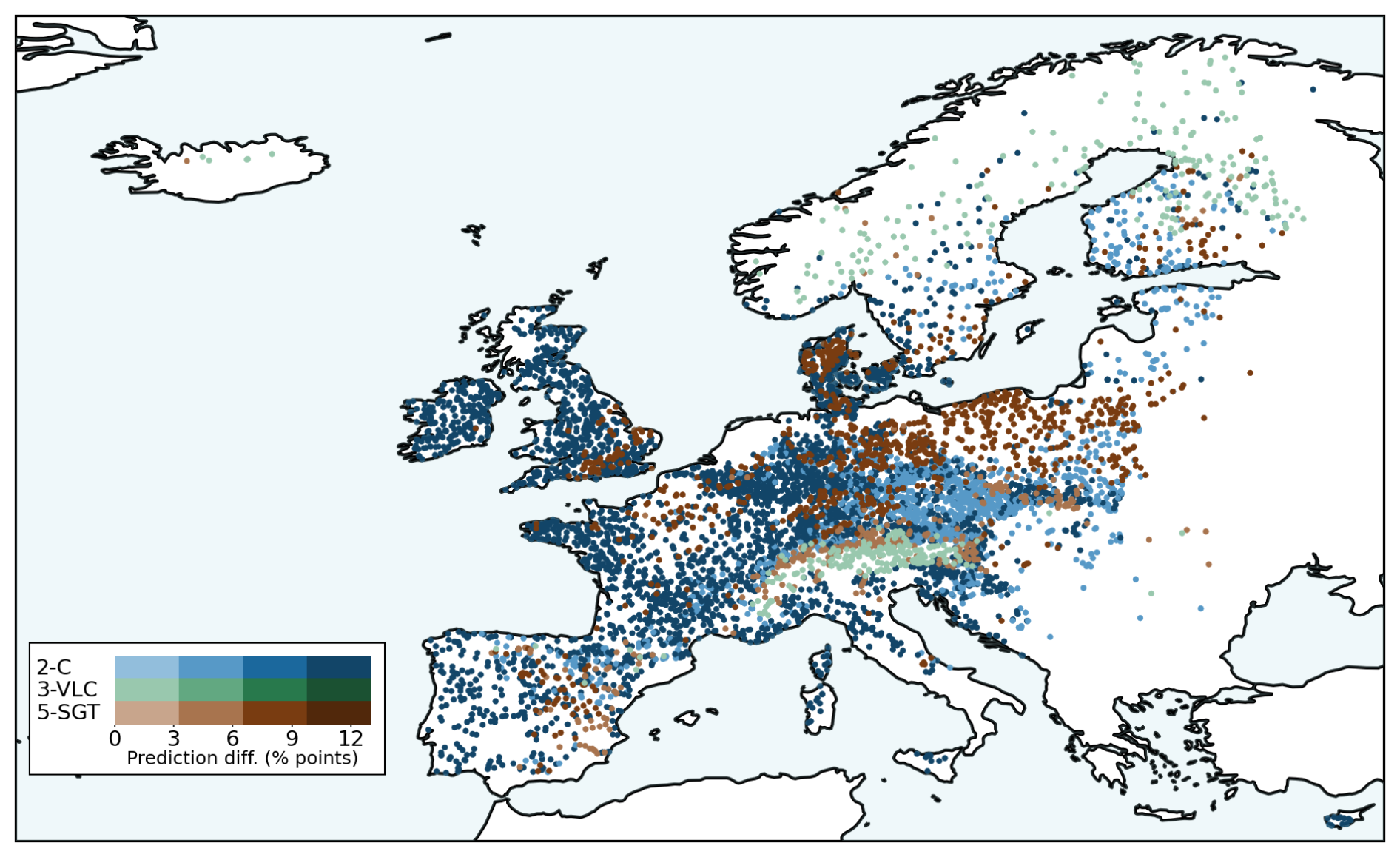
Figure 11 The map shows, for each HRT, which experiment achieved the highest proportion of correct predictions (indicated by colour). The colour intensity represents the magnitude of the difference between the highest and second-highest prediction accuracy: lighter colours indicate a small difference, whereas saturated colours indicate a larger difference. For example, the lighter blue catchments in central and eastern Europe and southern Finland indicate that the difference between the two best-performing experiments is small, whereas the more saturated colours in the UK indicate a larger performance gap. The colour bar units represent the percentage-point difference between the best and second-best prediction accuracies.

Viewing these results in a broader context, we can spatially map the HRTs according to the attribute group that serves as their strongest predictor. In total, 4 out of the 10 HRTs were predicted equally well or better by landscape attributes than by climate attributes (Fig. 11). Together, this amounts to 3226 catchments, which is 45 % of the total dataset. Soil, geology and topography attributes emerge as the dominant drivers of hydrological response in low to middle-elevation regions in central-eastern Europe, corresponding to HRTs 1 (stable, weak, winter regime) and 3 (wet, moderate, summer regime). Other catchments in the same geographic region, but belonging to HRT 6 (transitional, moderate, spring regime), are more strongly influenced by vegetation attributes. Vegetation also emerges as the strongest driver for catchments in HRT 7 (wet, strong, spring regime), in the higher elevation region of the Alps and at high-latitude regions.

5 Discussion

5.1 Streamflow behaviour in Europe

With the aim to distinguish the rich, multi-dimensional intricacies of the hydrological response and to identify coherent groups of hydrological similarity across 7175 river catchments in Europe at a much higher level of detail than what is currently known (Kuentz et al., 2017), individual HRTs were defined by 40 signatures of averages and inter-annual variability of streamflow magnitudes, timing and dynamics. In contrast to the initial expectations and somewhat surprisingly given the amount of data underlying the analysis, the k-means clustering method used here did not provide sufficient evidence to distinguish more than 10 individual classes of HRTs. These individual HRTs effectively only capture rather broad systematic differences between different response types at the continental scale. As the study domain is limited to Europe, these patterns reflect the variability of climatic and landscape conditions present in the region and may differ in areas with other environmental gradients. Within-HRT variability of the individual signatures remains pronounced (Figs. 4 and S2) and comparable to previous studies (e.g., Berghuijs et al., 2014). Each HRT shows low variability for some signatures and high variability for others, indicating that the HRTs represent certain aspects of hydrological behaviour well, while remaining broad or diffuse in others.

For example, HRT 7 (wet, strong, spring regime) is one of the most distinct classes, yet it exhibits large variability in the 30 d autocorrelation ($H_{{\mathrm{AC}}_{\mathrm{30}}}$), rising limb density (H_RLD), and days between highest and lowest flow ($H_{N(Q_{\mathrm{H}}-Q_{\mathrm{L}})}$) (Fig. 4g, h, j), while showing very little variability in the slope of the flow duration curve (H_FDC) (Fig. 4b). HRT 10 (dry, intermittent, winter regime), another well-defined HRT, has, on the other hand, one of the largest variability in the slope of the flow duration curve (H_FDC), but less variability in timing of low flow ($H_{t\left(Q_{\mathrm{L}}\right)}$) and 30 d autocorrelation ($H_{{\mathrm{AC}}_{\mathrm{30}}}$). Similar variation in the hydrological signatures is also seen in the less distinct classes such as HRT 2 (transitional, low, multi-seasonal regime), which exhibit less variability in rising limb density (H_RLD) and high variability for the baseflow index (H_BFI) (Fig. 4e, h). These heterogeneous patterns of within-class variability illustrate that general descriptions of the hydrological response characteristics that go beyond the major contrasts between the 10 HRTs, remains challenging. The key hydrological signatures with the strongest contrasts and thus the highest discriminatory power between HRTs included the Gini coefficient H_GC, the baseflow index H_BFI, as well as H_Q and $H_{Q_{\mathrm{95}}}$ but also the half-flow day H_t(HFD) as measure of timing and the variances of the Gini coefficient H_V,GC and flow H_V,Q as measures of inter-annual variability (Figs. 4, 3d, and S2). The combined importance of metrics of intra-annual timing, dynamics, magnitude and inter-annual variability for the identification of HRTs underlines the multi-faceted nature of streamflow, which requires all these different aspects for a meaningful characterisation of (dis)similarity of the hydrological response. In line with these findings, it was found that several HRTs were well-defined and clearly distinct from others. This is in particular the case for HRTs 1 (stable, weak, winter regime) and 10, which represent the respective extremes of many of the hydrological signatures. While HRT 1 is characterised by a stable, groundwater-driven system with little seasonality and generally low magnitudes of flow, HRT 10 is a highly dynamic, intermittent regime with strong seasonal variations in flow. HRTs 6–9 are similarly well defined by contrasts in multiple signatures. Other HRTs are less clearly defined. For example, HRT 5 (transitional, moderate, winter regime) closely resembled the overall sample average across most signatures, making it challenging to interpret, a challenge also noted by Jehn et al. (2020). Attempting to solve this issue, we analysed the effect of reducing the number of HRTs from 10 to 6–9. However, this did not eliminate the less distinct groups but instead increased the within-cluster variability of the remaining HRTs (not shown). Illustrating the complexity of classification, this suggests that certain HRTs may represent transitional or mixed hydrological behaviours that cannot be systematically and clearly enough distinguished with the available data, as it is in these cases difficult to attribute cluster boundaries to a single or even a few dominant signatures. The challenges in classifying HRTs are similar to those reported by Knoben et al. (2018), who found that some clusters are difficult to discern because catchments share climatic conditions and lack between-cluster diversity, whereas in other cases, differences in climate do not translate into statistically distinct flow regimes. The overall spatial pattern of the 10 HRTs identified in our study is broadly consistent with Kuentz et al. (2017), who identified 11 clusters of hydrological similarity across Europe. Some of the most distinct HRTs are similar, such as the high average flow, dynamic (i.e. low H_BFI) spring flow regime clustering on the west coast of the UK and Ireland (corresponding to our HRT 9 (wet, strong, early-winter regime)), the summer high flow regime of the Alps and wide parts of Scandinavia (our HRT 7) or the drier, more extreme regime with frequently intermittent flow in the Mediterranean regions (our HRT 10). However, differences in catchment sample size and signature selection lead to differences in other HRTs and limit further direct comparison.

A key feature of our results is that while a few HRTs are characterised by rather sharply defined geographic associations, such as the Alps and Scandinavia (HRT 7 (wet, strong, spring regime)) or the British Isles (HRT 9 (wet, strong, early-winter regime)), others extend over wide parts of Europe, some even spanning from southern Spain to northern Finland (e.g. HRT 6 (transitional, moderate, spring regime)). As a major implication, this demonstrates that spatial proximity, even across larger regional scales, is a poor predictor of streamflow behaviour. It also contrasts with earlier studies (Sawicz et al., 2011; Knoben et al., 2018; Brunner et al., 2020), where spatial proximity was reported to play a stronger role, and clusters tended to correspond to regions with similar climatic conditions or physical likeness. One potential reason is that those studies included climatic descriptors for clustering hydrological response types, whereas our classification approach was exclusively based on hydrological signatures.

5.2 Drivers of streamflow behaviour

In six individual experiments, membership of individual catchments to one of the 10 HRTs was predicted based on climate- and/or landscape attributes with the aim to identify the dominant drivers of streamflow behaviour. While this allowed to capture the major continental pattern, the overall prediction performances were rather modest, with accuracies not exceeding 0.69 for training and 0.59 for testing, respectively (Fig. 7). These levels of performance are comparable to previous studies. For example, Kuentz et al. (2017) reported that 60 % of catchments in Europe were correctly classified in their approach. In contrast, McManamay et al. (2014) and Brunner et al. (2020) reported lower errors (∼10 %) for predictions of correct regime class, although based on much smaller samples of catchments (<850) in the United States.

At the level of the individual HRTs, the prediction accuracies varied across all experiments. HRT 7 was throughout the best predicted with Acc_test=0.81–0.90, due to its distinct snowmelt-driven regime. HRTs 1 and 8–10 were also consistently well predicted with climate- and landscape attributes, mirroring the same HRTs that were most clearly defined by hydrological signatures. In contrast, HRT 5 is the worst-predicted cluster in all the experiments and at the same time the least well-defined cluster in terms of contrasts in hydrological signatures. Similar difficulties were seen for HRTs 2–4 and 6, which appear to be transitional classes, with mixing features of other HRTs. Confusion matrices for the experiments further revealed systematic misclassification among these less distinct HRTs (Fig. 8). This is consistent with earlier work suggesting that weak between-HRT diversity complicates the predictions (Knoben et al., 2018; Jehn et al., 2020), making it challenging to capture the essence of what is driving those clusters, at least at a continental scale. On the other hand, these HRTs have catchments distributed across multiple climate regions (from southern Spain to northern Nordics), indicating that similar hydrological response patterns can emerge under differing climatic conditions. This does not necessarily imply that landscape characteristics are more important than climate but rather suggests that similar hydrological behaviour can arise from different combinations of climatic and landscape controls. This is consistent with the concept of equifinality and uniqueness of place (Beven, 2000), where different processes or conditions can lead to comparable hydrological responses. Our Random Forest results support this interpretation, as both climate and landscape variables contribute to predictive skill across experiments. It could be reasoned that reducing the number of total HRTs would also limit the choice of the model, resulting in these “bland” catchments being lumped together into a more distinguishable and thus better predictable group. However, this was not the case, as in all experiments run with a reduced number of 6–9 HRTs, the less distinct clusters were preserved and the prediction accuracies were not substantially increased (Fig. S4), highlighting the inherent ambiguity in these HRTs.

The overall prediction accuracy Acc_test=0.55–0.61 (Fig. 7a) of experiment 2-C based on climate attributes underlines the important role of climate as driver of streamflow behaviour. However, the experiments based on landscape attributes resulted in only slightly lower accuracies with Acc_test<0.52. In addition, it was also found that landscape attributes can predict membership to HRTs at least as good or even better than climate attributes for 4 out of 10 HRTs (Fig. 11), with a total of 3226 catchments (45 %). In low- to mid-elevation regions of central-east Europe, soil, geology and topography related attributes are the most dominant controls of the hydrological response (HRTs 1, 3). Similarly, vegetation attributes emerge as strong controls in these regions (HRT 6), but notably also in the higher elevation region of the Alps and at higher latitudes (HRT 7). The importance of landscape as driver of the hydrological response is further exacerbated by the ranked importances of the attributes in experiment 1-CL (Fig. 10a). While climate attributes rank the highest, around half of the top 20 predictors are landscape attributes. In contrast to several studies that conclude that climate controls the hydrological response to a large extent with only limited landscape influence (Kuentz et al., 2017; Beck et al., 2015; Addor et al., 2018), our results provide broad empirical evidence supporting other previous studies that argue that landscape exerts a stronger influence than often assumed, in particular in specific regions (Knoben et al., 2018; Dal Molin et al., 2020; Almagro et al., 2024; Araki et al., 2026).

In light of our results, it can be argued that the frequently adopted climate vs. landscape perspective may lead to an overly simplistic perception of the system. This is for example illustrated by the dominant attributes that emerge in the landscape-only experiments 3-VLC (Fig. 10c) and 5-SGT (Fig. 10e). In 3-VLC, metrics of both inter-annual variability (V_V,NDVI) and seasonality ($V_{R\left({\mathrm{NDVI}}_{\mathrm{Parde}}\right)}$) were in the top-ranking attributes. Both are direct imprints of climatic conditions on the landscape over rather short time scales. Similarly, the fraction of tree cover (V_F(TC)) as well as the elevation (T_Elev) as further key attributes in 3-VLC and 5-SGT, respectively, reflect aggregate effects of different temperature regimes across elevational gradients, although correlation with individual climate attributes such as the fraction of snow C_F(Snow) is very limited (R²=0.09). These examples illustrate that landscape attributes are to a certain extent shaped by climate, thus also containing information on climatic conditions. It is therefore argued that the climate vs. landscape dichotomy is false and should be replaced by a climate and landscape perspective that explicitly accounts for the interactions in and co-evolution of the overall system (e.g., Savenije, 2010; Troch et al., 2013, 2015).

Spatial autocorrelation

When using a large dataset spanning Europe, neighbouring catchments are more likely to exhibit similar behaviour in terms of hydrology, but also in climate and landscape. This, in turn, could have an influence on the hydrological clustering as well as potentially yielding more optimistic Random Forest classification results. Moran's I is a measure for spatial autocorrelation, and was calculated for each Random Forest experiment as a first step in quantifying the spatial autocorrelation. Values of I∼0.3 were found, indicating a degree of spatial correlation consistent with previous studies (e.g., Addor et al., 2018). The spatial autocorrelation is difficult to meaningfully deal with because it is inherent in any type of hydrological clustering, as most of the signatures are affected by climate and landscape, which have very local and regional similarities. To further disentangle the effect of spatial autocorrelation, a 10-fold spatial block cross-validation was run in the Random Forest analysis. In this approach, catchments were partitioned into contiguous spatial blocks (e.g. training set: catchments in the south-west, testing: catchments in the north-east of the domain) rather than randomly sampled. While training accuracies remained largely the same, testing accuracies decreased as compared to the original analysis (Fig. S13 in the Supplement). However, the hierarchy of drivers remained largely the same, as for example HRT 1 performs best in the soil, geology and topography experiment (5-SGT), while HRT 7 is still largely driven by vegetation and landcover attributes (Fig. S14). These results suggest that the performance decrease under spatial block cross-validation likely reflects a combination of two effects. On the one hand, spatial blocking introduces a distributional mismatch between training and test sets, as spatially neighbouring catchments tend to share similar climate and landscape characteristics, meaning the model is evaluated on conditions that are underrepresented or absent during training. On the other hand, it remains plausible that spatial autocorrelation contributes to some degree of inflated performance under random cross-validation, given that spatially proximate catchments are more likely to have the same hydrological regime membership. Disentangling these two effects is non-trivial, and both mechanisms likely contribute to the observed performance drop. Nevertheless, the substantial decrease in test accuracy under spatial block cross-validation is consistent with the interpretation that spatial proximity carries predictive information not fully represented by the available climate and landscape attributes, suggesting that under random cross-validation, the model may partly rely on spatial covariance structures that are not fully resolved by the available attributes. This, in turn, highlights the challenge of disentangling hydrological drivers across regions with strong spatial structure, and underlines that currently available data are largely insufficient to resolve the “uniqueness of place” (Beven, 2000) in a meaningful way.

5.3 Limitations and future work

The spatial distribution and quality of the underlying data represent a source of uncertainty in this study. Streamflow observations are unevenly distributed across Europe, with a high density of gauged catchments in central Europe and lower coverage in the eastern and southern regions (do Nascimento et al., 2024). This imbalance may lead to an overrepresentation of hydrological characteristics of well-monitored regions, potentially limiting the representation of more data-scarce areas. In addition, the meteorological forcing is derived from the E-OBS dataset, whose accuracy similarly depends on station density and varies spatially. In regions with lower station density, particularly in parts of southern and eastern Europe, precipitation may be underestimated (Clerc-Schwarzenbach and do Nascimento, 2026). This may influence the derived climatic attributes and, consequently, their relationship with hydrological response. Despite the limitation in station density and uncertainty in the meteorological data, the dataset is considered sufficiently robust for identifying large-scale patterns across Europe (Clerc-Schwarzenbach and do Nascimento, 2026).

It should be noted that there exists potential multicollinearity among the hydrological signatures and climate and landscape attributes. As the aim of the study was to retain a broad set of signatures and attributes, no extensive variable selection was applied to minimise redundancy. Instead, a Pearson correlation-based pre-filtering step was used to remove highly correlated variables ($\left|r\right|>\mathrm{0.75}$). This resulted in 50 % of the hydrological signatures and climate and landscape attributes exhibiting r<0.12 (equivalent to explaining ∼1 % of the variance) and only 2.5 % of the attributes being correlated with r>0.6 (explaining 36 % of the variance; see Fig. S1). Some correlation remains, and to explicitly test the robustness of the model interpretation, the consistency of the feature importance ranking of the climate and landscape attributes across experiments was evaluated (Fig. S12). The most influential variables show broadly consistent rankings across model configurations, suggesting that the main conclusions are not sensitive to multicollinearity effects. Nevertheless, correlated predictors may still affect the attribution of importance and comparisons between experiments with different predictor sets.

The presence of nested catchments may introduce dependencies that influence the cross-validation in the Random Forest experiments. To assess the impact of nested catchments on the results, the analysis was repeated with a subset of non-nested catchments (n=4137). The results show that both the clustering into hydrological response types and the Random Forest classification performance remain largely unchanged (Figs. S15, S16 and S17), with only a small decrease in testing accuracy (1 %–5 % across experiments, Fig. S17). These results indicate that, while nesting introduces some dependence, its influence on the overall clustering and classification results is sufficiently limited for the purpose of this analysis.

There are also methodological limitations related to the use of k-means clustering to group catchments into hydrological response type groups (HRTs) based on 40 hydrological signatures. k-means relies on rigid cluster boundaries and assigns equal weight to all signatures, which may not reflect the actual complexity of hydrological systems. This limitation is reflected in the weak elbow (Fig. 2) and consistently low Silhouette Scores across the range of cluster numbers, indicating limited separability in the data. The PCA results also show that a relatively large number of principal components are required to explain most of the variance, suggesting that the signatures do not form clearly distinct groups in feature space. This may partly reflect the system complexity, where hydrological behaviour varies continuously and overlaps in multidimensional space, rather than forming discrete groups (McManamay et al., 2014; Knoben et al., 2018).

Several directions for future research can be derived from the above reflections. First, further work should aim to disentangle the relative roles of landscape by analysing subsets of catchments within more homogeneous climatic regions. Second, the present analysis is based on long-term aggregated statistics and does not explicitly account for temporal dynamics beyond inter-annual variances. Future studies should investigate changes in hydrological response over time, for example, by analysing different climatic periods or assessing the impacts of climate change. Third, alternative clustering approaches that allow for more flexible or overlapping group structures (e.g. fuzzy or hierarchical clustering) could be explored to better capture the continuous nature of hydrological variability. Finally, continued development of spatially explicit modelling and validation approaches may help to better account for spatial autocorrelation in large-sample hydrological studies.

5.4 Wider implications

Overall, this study demonstrates that even the use of an unprecedented range of data does not allow to systematically characterise and robustly identify more than 10 broad types of hydrological response classes across Europe, and to narrow down the within-class variability. The question of what constitutes the hydrological response and (dis)similarity therein thus remains largely unresolved. Similarly, the modest accuracies to predict membership to the 10 HRTs based on a wide spectrum of climate- and landscape attributes illustrates that the question what drives the hydrological response remains equally unresolved. In other words, a satisfactory and generalisable answer to the question “Why do we in a specific catchment observe a specific flow magnitude at a specific moment, and why is it different to the flow in other catchments at other moments?” is still lacking. Ultimately, the results of this study underline that available data are still insufficient to describe the complexity of the hydrological system, highlighting the need for considerably more data with higher spatial and temporal resolution and observational detail. This further suggests that Beven's “uniqueness of place” (Beven, 2000) is a larger obstacle to generalisation in hydrology than previously thought and that this postulate is more relevant than ever.

6 Conclusions

The aim of this study was to (1) realise a detailed classification of hydrological response types (HRTs) with minimal intra-class variance by using a large catchment sample and a wide range of hydrological signatures, including descriptors of inter-annual variability, and (2) to identify the dominant drivers of streamflow behaviour, and in particular whether climate, rather than landscape exert more discriminatory power to explain the dissimilarity between the identified HRT classes.

Our results showed that, classifying 7175 catchments across Europe, using 40 hydrological signatures describing averages, inter-annual variability of streamflow magnitudes, timing, duration, frequency, and seasonality, no more than 10 HRTs could be meaningfully distinguished. Even with this level of detail, the HRTs could only capture broad patterns of the hydrological response. The most distinct HRTs typically contained catchments with strong seasonal or extreme flow regimes. Others were more difficult to define, as they overlapped in terms of average characteristics with the other HRTs.

Climate consistently emerged as the dominant driver of streamflow behaviour when 84 climate- and landscape attributes were used to predict catchment membership to the 10 HRTs. However, landscape attributes represent half of the 20 most important drivers of the hydrological response. In addition, in 4 out of the 10 HRTs, landscape was found to be as strong or even stronger a control than climate. This highlights that the landscape characteristics, often reported as having little influence on the differences in hydrological behaviour at continental scales, plays a much more important role than frequently thought.

Overall, the results of this study demonstrate that the “uniqueness of place” concept (Beven, 2000) remains highly relevant, and provide further evidence that more consideration needs to be given to the perspective of co-evolution between climate and landscape in shaping hydrological behaviour at continental scales.