Capturing the extremes: a quasi-comonotonicity-based algorithm for disaggregating daily to hourly rainfall

Disaggregating daily precipitation data into hourly time scales is crucial for hydrological modelling, urban drainage design, and extreme rainfall risk assessment. This study presents Q-CODA, a novel Quasi-COmonotonicity-based Disaggregation Algorithm that leverages the quasi-comonotonic relationship between daily precipitation totals and their sub-daily maxima to generate hourly rainfall sequences consistent with observed extremes. The method combines a Fréchet–Hoeffding upper bound copula to constrain sub-daily maxima with a K-nearest neighbours approach and an iterative adjustment algorithm to ensure consistency with daily totals and multiple sub-daily constraints. Q-CODA is evaluated through a 5-fold cross-validation over 91 meteorological stations across Spain (1996–2024) and compared against state-of-the-art methods, including nearest-neighbour resampling, Poisson cluster models, multiplicative cascades, and deep learning approaches. Results show that Q-CODA consistently outperforms state-of-the-art methods in reproducing extremes. Across stations, median values indicate a 1-D Wasserstein distance of 0.015 compared to 0.021–0.073, and a bias in the 99.9th percentile of −2.8 % versus −29 % to +11 %. Temporal structure is also well preserved, with event duration bias of −2.0 % (vs. −22 % to +13 %) and lag-1 autocorrelation bias of −4.4 % (vs. −37 % to −7.8 %). For intensity-duration-frequency curves, Q-CODA attains a median root mean square error of 1.16 mm h⁻¹ for a 100-year return period, improving upon the 1.62–4.60 mm h⁻¹ range of alternative methods. Additional analyses across other climate regimes, including the Pacific Northwest and Florida (United States), show consistently strong performance, indicating stable and reliable behaviour under varying climatic conditions. Furthermore, a semi-parametric regionalised extension enables application at ungauged locations while maintaining competitive accuracy. Overall, Q-CODA provides a consistent and transferable framework for sub-daily rainfall disaggregation with clear advantages for extreme-value representation and hydrometeorological applications.

1 Introduction

Rainfall is one of the most variable components of the hydrological cycle, exhibiting pronounced fluctuations across spatial and temporal scales. While sub-hourly or hourly rainfall data are essential for simulating surface runoff, designing urban drainage infrastructure, and assessing flood risks (Schilling, 1991; Fowler et al., 2021; Haslinger et al., 2025), such high-resolution records are often unavailable or incomplete due to technical and logistical constraints. In contrast, daily precipitation measurements are widely available from global meteorological networks, leading to a growing demand for accurate temporal disaggregation methods that can transform daily totals into realistic sub-daily sequences (Takhellambam et al., 2022; Ebers et al., 2024).

Temporal disaggregation, also known as temporal downscaling, refers to the process of generating high-resolution time series from lower-resolution observations while preserving key statistical and hydrological characteristics. Traditional approaches to precipitation disaggregation can be broadly categorized into two families: stochastic rainfall generators and resampling-based methods. Stochastic generators such as Poisson cluster processes (Rodriguez-Iturbe et al., 1987; Onof et al., 2000; Qin and Dai, 2024) or Markov chain-based schemes (Stoner and Economou, 2020; Vorobevskii et al., 2024) simulate rainfall sequences by modelling the occurrence and intensity of rainfall events using probabilistic laws. While theoretically appealing, these models often require extensive calibration and may underperform in replicating extremes (Vorobevskii et al., 2024). Resampling-based methods such as K-Nearest Neighbors (KNN) and Methods of Fragments (MoF) disaggregation rely on analogues from historical high-resolution observations (Pui et al., 2012; Alzahrani et al., 2023). These approaches are nonparametric, easy to implement, and capable of preserving observed patterns; however, KNN and MoF methods can suffer from limitations including sensitivity to the choice of neighbours and potential mismatch lag-1 autocorrelation (Li et al., 2018).

To address some of these challenges and improve the realism of disaggregation, newer approaches such as the Microcanonical Multiplicative Random Cascade (MMRC) methodology and deep learning techniques have been increasingly explored. MMRC models disaggregate rainfall by recursively partitioning precipitation amounts into smaller time intervals using multiplicative random weights, preserving the overall mass while reproducing the multifractal and scaling properties of rainfall (Förster et al., 2016; Müller and Haberlandt, 2018; Müller-Thomy, 2020; Maloku et al., 2023). In parallel, deep learning methods have gained traction in rainfall disaggregation due to their ability to capture complex nonlinear dependencies (Scher and Peßenteiner, 2021; Bhattacharyya and Saha, 2023; Oates et al., 2025). Hybrid models combining Artificial Neural Networks (ANN) with K-means clustering algorithms (e.g., ANN-K) have shown promise in improving event-based performance and capturing nonlinear patterns. A recent study (Bhattacharyya et al., 2024) indicates that ANN-K produces better results in conserving extreme rainfall than MMRC and Neyman-Scott Rectangular Pulse (NSRP) processes. Nonetheless, such data-driven deep learning methods require large training datasets, risk overfitting, and often lack physical interpretability, making their generalization across climatic regions challenging.

A particularly persistent difficulty in temporal disaggregation is the adequate reproduction of extreme rainfall intensities and their temporal structure. Most existing methods either under-represent short-duration maxima or distort their alignment with daily totals, which can lead to substantial biases in hydrological simulations and impact assessments. This motivates the need for innovative strategies that explicitly account for the statistical dependence between daily and sub-daily precipitation features.

Copula theory (Sklar, 1996) provides a robust mathematical framework for modelling such dependencies, allowing the construction of joint distributions that preserve individual marginals while flexibly capturing inter-variable dependence. Copula-based models have been successfully applied to hydrological problems such as rainfall-runoff modelling, multivariate drought analysis, and spatial rainfall simulation (Naderi et al., 2022; Moradzadeh Rahmatabadi et al., 2023). However, previous copula-based approaches to rainfall modelling have primarily focused on capturing the statistical dependence between precipitation intensities at different temporal or spatial scales, or on modelling joint distributions of variables such as storm duration and depth (Vorobevskii et al., 2024; Biswas and Saha, 2025). These approaches have not explicitly leveraged the quasi-comonotonic relationship between sub-daily precipitation maxima (e.g., 1, 2 h intensities) and the corresponding daily total as a structural constraint in the simulation of high-resolution rainfall time series. This quasi-comonotonicity implies that extreme hourly accumulations tend to co-occur with large daily totals, imposing an upper limit on feasible sub-daily intensities.

In this study, we propose a novel assumption of the Fréchet–Hoeffding upper bound copula (Joe, 2005; Abdellatif et al., 2024), also known as comonotonicity copula, to simulate sub-daily maxima conditioned on daily totals, thereby generating physically plausible upper envelopes that act as dynamic, event-specific constraints. These constraints complement the daily total in guiding the subsequent disaggregation process and allow for the generation of hourly rainfall sequences that better preserve the magnitude and timing of extreme events. This methodological innovation constitutes the core contribution of our disaggregation framework and distinguishes it from existing statistical or deep learning-based approaches. In this context, we present Q-CODA (Quasi-COmonotonicity-based Disaggregation Algorithm), a novel precipitation disaggregation framework that leverages the quasi-comonotonic dependence between daily totals and sub-daily maxima to constrain and guide the generation of hourly rainfall series. The proposed method comprises three key components: (i) simulation of sub-daily maximum intensities assuming the Fréchet–Hoeffding upper bound copula conditioned on daily rainfall, (ii) seeding of initial hourly patterns using a K-Nearest Neighbours approach, and (iii) iterative adjustment to enforce consistency with daily totals and the simulated sub-daily maxima across multiple accumulation windows (1, 2, 6, and 12 h).

The remainder of this paper is organised as follows. Section 2 describes the dataset and study domain. Section 3 introduces the proposed Q-CODA framework, including the derivation of sub-daily constraints, the comonotonic transformation, and the iterative adjustment procedure. Section 4 presents the state-of-the-art disaggregation methods used for comparison. Section 5 outlines the evaluation strategy. Section 6 presents the results of the evaluation. Section 7 provides a detailed discussion of the findings, assesses the method's performance across diverse climatic regimes including international datasets, and introduces an expansion of the algorithm for spatial applications. Section 8 summarizes the main conclusions. Additionally, supplementary material provides information and detailed analyses that complement the preceding sections.

2 Data and Study Area

This study leverages a high-quality, high-resolution precipitation dataset from 91 meteorological stations maintained by the Spanish State Meteorological Agency (AEMET). The selected stations are distributed across the Iberian Peninsula and the Balearic Islands, ensuring extensive spatial coverage across diverse climatic zones of Spain (see Fig. 1). The dataset spans a 29-year period (1996–2024), with hourly precipitation records available at 0.1 mm resolution. Only stations with at least 90 % hourly data completeness were retained to ensure data robustness and minimize biases introduced by missing values. Annual data completeness can be consulted in Fig. S1 in the Supplement. The geographic diversity of the station network covers coastal, mountainous, and inland regions, as well as areas subject to Mediterranean, Atlantic, and continental climatic influences. This variability in hydroclimatic regimes, ranging from convective summer storms to winter frontal systems, provides a rigorous testbed for evaluating the performance and generalizability of the proposed Q-CODA disaggregation framework across multiple rainfall-generating mechanisms. Importantly, the scale of this study sets it apart from many recent rainfall disaggregation studies that rely on significantly smaller station networks, often basing methodological conclusions on fewer than 10 sites (e.g., Lee et al., 2022; Bhattacharyya et al., 2024; Chowdhury et al., 2025). Such limited spatial sampling can hinder the generalization of results, particularly in regions with high climate variability. By contrast, our analysis aligns with recent best practices emphasizing broad spatial validation and data diversity (e.g., Müller-Thomy, 2020; Ebers et al., 2024), which are crucial for evaluating the robustness of disaggregation methods across different hydrometeorological contexts.

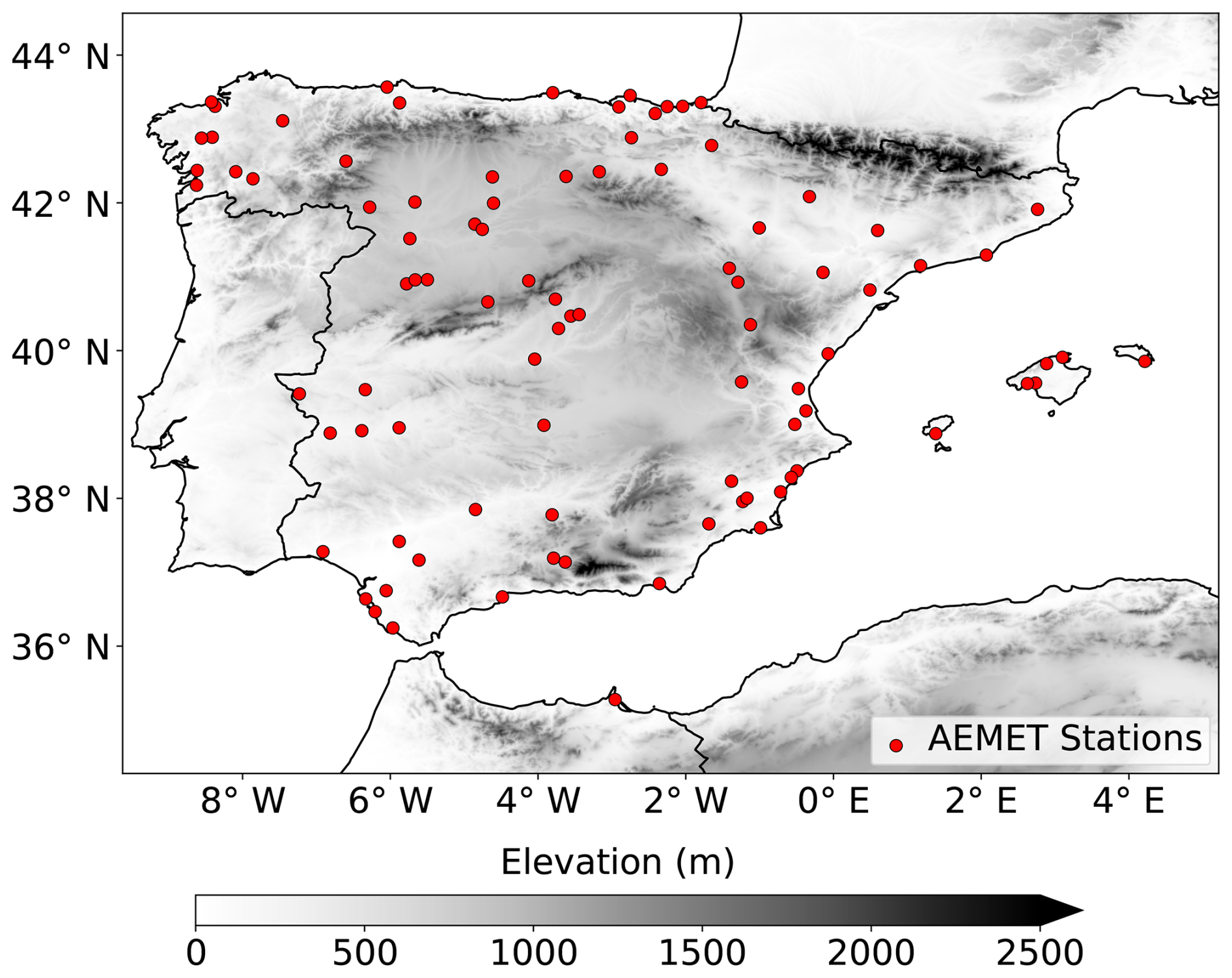
Figure 1 Map showing the location of AEMET stations with available hourly precipitation records used in this study (elevation data: NOAA 2022; https://doi.org/10.25921/fd45-gt74, NOAA National Centers for Environmental Information, 2022).

For visualization, Fig. 1 shows the geographic location of the 91 stations used in the analysis, highlighting the spatial representativeness of the dataset. All data were subjected to a thorough quality control process and days with clearly erroneous or missing hourly values were excluded from the analysis. In addition, a homogeneity assessment was performed on annual precipitation series derived from the hourly data using the Pettitt test, the Standard Normal Homogeneity Test, and the Buishand range test, using a significance level of 0.05. A spatial consistency check with neighboring stations (within 50 km) was also conducted. Results indicated that 86 of the 91 stations showed no evidence of inhomogeneities. The few flagged cases were clustered in northern Spain and linked to anomalously wet periods rather than documented station changes, suggesting false positives due to natural variability. These stations did not correspond to outliers in the evaluation, indicating no impact on the interpretation of results. The full hourly time series were used to derive both daily precipitation totals (for disaggregation input) and sub-daily maxima over selected accumulation durations (1, 2, 6, and 12 h), which served as internal constraints and evaluation targets throughout the disaggregation framework.

3 Methodology

3.1 Conceptual Framework

Temporal disaggregation of daily precipitation into sub-daily time scales relies fundamentally on capturing the strong dependence between daily precipitation totals and sub-daily maxima. Empirical evidence shows a quasi-comonotonic relationship between these variables, meaning that high sub-daily maxima tend to coincide with large daily totals. This near-perfect positive dependence provides a natural constraint for disaggregation, ensuring physically plausible rainfall sequences.

Copulas are functions that couple multivariate distribution functions to their univariate marginals, enabling flexible modelling of dependence structures independently of marginal behaviour. Formally, for random variables X and Y with marginal cumulative distribution functions (CDFs) F_X(x) and F_Y(y), Sklar's theorem (Sklar, 1996; Joe, 2005; Abdellatif et al., 2024) states that there exists a copula C such that the joint CDF $F_{X,Y}(x,y)$ can be expressed as:

$$\begin{array}{}\text{(1)}& F_{X,Y}(x,y)=C\left(F_X\right(x),F_Y(y\left)\right).\end{array}$$

The copula $C:[\mathrm{0},\mathrm{1}{]}^{\mathrm{2}}\to [\mathrm{0},\mathrm{1}]$ encapsulates the dependence structure between X and Y.

Among the family of copulas, the Fréchet–Hoeffding bounds define the theoretical limits of dependence. The upper bound copula C⁺, representing perfect positive dependence (comonotonicity), is defined as:

$$\begin{array}{}\text{(2)}& C^{+}(u,v)=min(u,v),\end{array}$$

for $u,v\in [\mathrm{0},\mathrm{1}]$.

This copula implies that X and Y increase together surely, which aligns approximately with the quasi-comonotonic behaviour observed between daily precipitation totals and sub-daily maxima. Assuming the Fréchet–Hoeffding upper bound copula allows us to generate the upper envelope or conditional upper bound of sub-daily maxima given daily totals. This approach provides a dynamic constraint that complements the daily precipitation total by restricting the range of possible sub-daily intensities to those consistent with observed extreme behaviour. Unlike previous rainfall disaggregation approaches (KNN, ANN-K, MMRC, Poisson-cluster models, and other copula-based frameworks), which represent the dependence between daily totals and sub-daily maxima in a purely statistical manner without explicit structural constraints, our method exploits their quasi-comonotonic relationship as a key structural feature. This enhances the physical realism of simulated hourly sequences, especially for extreme events, by ensuring that sub-daily maxima do not exceed plausible bounds conditional on the daily total. To illustrate this quasi-comonotonic dependence, we include Fig. 2 showing the empirical Spearman rank correlation coefficient (ρ_S) between sub-daily precipitation maxima aggregated over different time windows ($P_{\mathrm{t}}^{\text{max}}$) and the corresponding daily total precipitation (P_d).

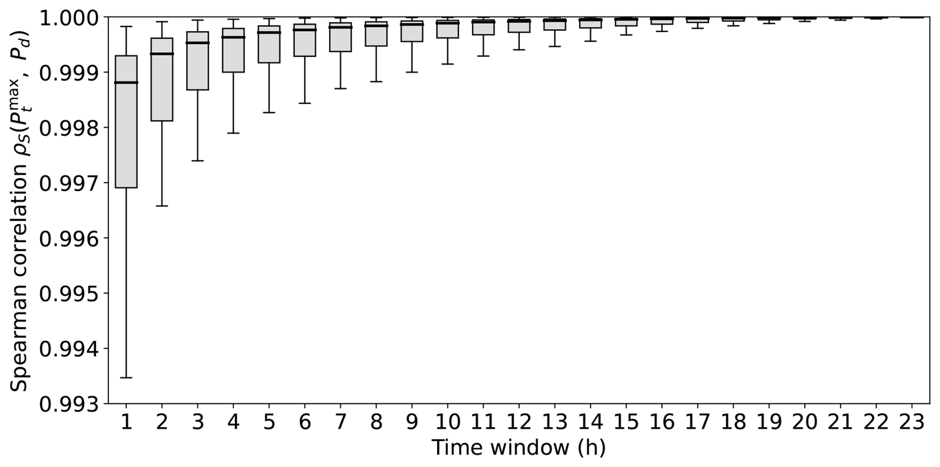
Figure 2 Spearman rank correlation coefficient (ρ_S) between sub-daily precipitation maxima aggregated over varying time windows ($P_{\mathrm{t}}^{\text{max}}$) and the corresponding daily total precipitation (P_d). Each boxplot summarizes the distribution across the 91 stations.

Figure 2 clearly shows empirical values of Spearman correlation approaching 1, confirming the near-perfect positive dependence, though decreases slightly for shorter durations, reflecting the increasing variability of shorter accumulation periods. This figure visually supports the theoretical basis of our methodology by quantifying the strength of the dependence exploited through the Fréchet–Hoeffding upper bound copula.

In this study, the Fréchet–Hoeffding upper bound copula is not assumed to represent the exact dependence structure between daily precipitation totals and sub-daily maxima. Rather, it is used to define an idealized limiting case corresponding to perfect positive dependence (comonotonicity), which provides a useful theoretical reference for constructing physically consistent constraints during the disaggregation process. Empirical analyses (see Fig. 2) show that daily totals and sub-daily maxima exhibit a very strong but not perfectly monotonic relationship. We therefore refer to this behaviour as quasi-comonotonic: large daily totals are consistently associated with large sub-daily maxima, although variability remains due to event structure and timing. Within Q-CODA, the upper bound copula is used as a practical mechanism to translate this near-monotonic relationship into conditional target values for sub-daily extremes. These targets do not impose a deterministic mapping but instead provide an upper-envelope constraint that guides the reconstruction toward solutions that are statistically consistent with the observed dependence structure.

3.2 Sub-daily Maximum Simulation

Following the conceptual framework introduced in Sect. 3.1, the Fréchet–Hoeffding upper bound copula is accepted to simulate physically consistent sub-daily maximum precipitation intensities conditioned on daily totals. This step provides a set of dynamic constraints that ensure physically plausible short-duration rainfall intensities during the disaggregation process.

Let P_d denote the daily precipitation total and $P_{\mathit{\tau }}^{\text{max}}$ the maximum accumulated precipitation over a sub-daily windows of duration $\mathit{\tau }\in \mathit{\{}\mathrm{1}\mathrm{h},\mathrm{2}\mathrm{h},\mathrm{6}\mathrm{h},\mathrm{12}\mathrm{h}\mathit{\}}$. Assuming quasi-comonotonicity, the joint distribution of ($P_{\mathrm{d}},P_{\mathit{\tau }}^{\text{max}}$) is modelled using the Fréchet–Hoeffding upper bound copula C⁺, defined as:

$$\begin{array}{}\text{(3)}& F_{P_{\mathrm{d}},P_{\mathit{\tau }}^{\text{max}}}(x,y)=min\left(F_{P_{\mathrm{d}}}\right(x),F_{P_{\mathit{\tau }}^{\text{max}}}(y\left)\right).\end{array}$$

Given a daily total P_d=x, we aim to simulate the corresponding sub-daily maxima $P_{\mathit{\tau }}^{\text{max}}$ such that the pair $(x,P_{\mathit{\tau }}^{\text{max}})$ lies on or below the upper copula bound. Since C⁺ corresponds to perfect rank correlation, the conditional distribution of $P_{\mathit{\tau }}^{\text{max}}|P_{\mathrm{d}}=x$ can be approximated via comonotonic transformation, Eq. (4):

$$\begin{array}{}\text{(4)}& P_{\mathit{\tau }}^{\text{max}}=F_{P_{\mathit{\tau }}^{\text{max}}}^{-\mathrm{1}}\left(F_{P_{\mathrm{d}}}\right(x\left)\right),\end{array}$$

where $F_{P_{\mathrm{d}}}$ and $F_{P_{\mathit{\tau }}^{\text{max}}}$ are the empirical cumulative distribution functions (ECDFs) estimated from historical in each climatological season (DJF, MAM, JJA, or SON). This formulation enforces a strong dependence structure between daily totals and sub-daily peaks, while preserving the observed marginal distributions. For each simulated day, a vector of conditional maxima $\mathit{M}=(P_{\mathrm{1}\mathrm{h}}^{\text{max}},P_{\mathrm{2}\mathrm{h}}^{\text{max}},P_{\mathrm{6}\mathrm{h}}^{\text{max}},P_{\mathrm{12}\mathrm{h}}^{\text{max}})$ is generated, where $P_{\mathit{\tau }}^{\text{max}}$ denotes the maximum allowable precipitation over a sliding window of duration τ, consistent with the observed comonotonic relationship. These constraints are subsequently enforced in the disaggregation process (see Sect. 3.4), ensuring that simulated hourly series are consistent with both the daily total and realistic sub-daily intensities. This step is essential to preserve the magnitude and timing of extreme sub-daily events, which are critical for hydrological applications such as flood modelling, urban drainage, and climate impact assessment.

To evaluate the suitability of assuming the upper copula C⁺ to estimate M via comonotonic transformation, defined in Eq. (4), we compared its performance against Isotonic Regression (IR), a standard non-parametric machine learning method that fits monotonic functions without assuming a specific functional form (De Leeuw, 1977; Chakravarti, 1989; Delong and Wüthrich, 2024). Its use as a reference is particularly relevant here, as both IR and the Comonotonic Transformation (CT) rely on the monotonicity assumption, albeit from different theoretical foundations: IR enforces monotonicity through piecewise-constant regression fits, while CT exploits comonotonicity explicitly via copula theory. Both approaches were trained and tested using a consistent 5-fold cross-validation scheme, applied independently at each station. To ensure reproducibility, we used the same non-overlapping temporal folds defined in Sect. 5, where hourly disaggregation performance is evaluated in detail. Figure 3 presents the bias (%) in estimating the 99th percentile of observed sub-daily maxima for each duration in the constraint vector M, aggregated across 91 stations.

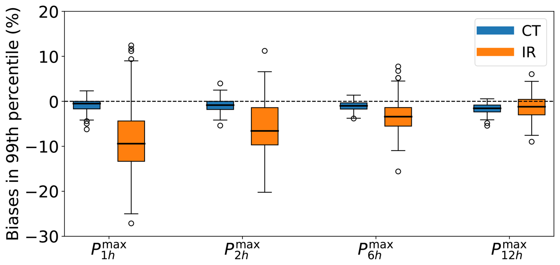
Figure 3 Bias (%) in estimating the 99th percentile of observed sub-daily precipitation maxima for each duration included in the constraint vector M, aggregated across 91 stations.

While IR can adapt to nonlinearities in the data, it struggles to accurately capture the tail behaviour of precipitation distributions. The CT consistently achieves lower biases compared to IR, with the differences being more pronounced at shorter aggregation durations, indicating a closer match to the empirical distributions of extreme short-duration rainfall. These distributional advantages make CT a more appropriate choice for integrating sub-daily intensity information into the disaggregation framework, as detailed below.

3.3 Initial Pattern Seeding via KNN

To generate an initial realistic sub-daily precipitation pattern consistent with a given daily total (P_d), we employ a K-Nearest Neighbours (KNN) approach. For each target day in the test set, we identify historically observed daily events from the training set with similar P_d magnitudes, constrained to the same climatological season (DJF, MAM, JJA, or SON). Specifically, since only one predictor (daily total precipitation) is used, the Euclidean distance (between the target daily total $P_{\mathrm{d}}^{\text{target}}$ and each candidate training value $P_{\mathrm{d},i}^{\text{train}}$ within the same season) reduces to the absolute difference:

$$\begin{array}{}\text{(5)}& d_i=|P_{\mathrm{d}}^{\text{target}}-P_{\mathrm{d},i}^{\text{train}}|.\end{array}$$

The set of neighbours is then defined as the indices corresponding to the k smallest distances:

$$\begin{array}{}\text{(6)}& {\mathcal{N}}_k=\text{argsort}(d{)}_{i:k},\end{array}$$

where k=10. From this set, a single neighbour j∈N_k is randomly selected with equal probability.

The associated hourly precipitation pattern $\mathit{h}=(h_{\mathrm{1}},h_{\mathrm{2}},\mathrm{\dots },h_{\mathrm{24}})$ of the selected neighbour j is scaled proportionally to match the target total:

$$\begin{array}{}\text{(7)}& \mathit{h}\leftarrow \mathit{h}\times {\displaystyle \frac{P_{\mathrm{d}}^{\text{target}}}{{\sum }_{i=\mathrm{1}}^{\mathrm{24}}{h}_i}}.\end{array}$$

This scaled pattern constitutes the initial seeding for the iterative refinement described in Sect. 3.4, which adjusts sub-daily intensities to meet prescribed constraints on maxima over multiple accumulation intervals.

3.4 Iterative Adjustment Procedure

Conceptually, the method operates in percentile space. For each wet day, the target daily precipitation total is first located within the empirical distribution of daily totals derived from the training data. Under the assumption of comonotonic behaviour, the same percentile is then used to infer a corresponding target value for the sub-daily maximum precipitation from its empirical cumulative distribution function. This step is equivalent to applying the Fréchet–Hoeffding upper bound, which links the marginal distributions through a shared rank structure. The resulting target maximum is subsequently used as a constraint within the iterative adjustment procedure to ensure that the reconstructed hourly sequence is consistent with both the daily total and the expected magnitude of sub-daily maxima.

Starting from the obtained initial hourly precipitation vector h via KNN and target constraints composed of the daily total precipitation P_d and the obtained sub-daily maxima vector M via CT, the iterative adjustment procedure modifies h to satisfy these constraints simultaneously. At each iteration, for each aggregation duration $\mathit{\tau }\in \mathit{\{}\mathrm{1}\mathrm{h},\mathrm{2}\mathrm{h},\mathrm{6}\mathrm{h},\mathrm{12}\mathrm{h}\mathit{\}}$, the procedure identifies the contiguous time window $I_{\mathit{\tau }}=\mathit{\{}i,\mathrm{\dots },i+\mathit{\tau }-\mathrm{1}\mathit{\}}$, where i is the starting hour of that window (ranging from 1 to 25−τ), for which the current sum is maximal.

$$\begin{array}{}\text{(8)}& S_{\mathit{\tau }}^{\text{max}}={max}_{i=\mathrm{1},\mathrm{\dots },\mathrm{25}-\mathit{\tau }}{\sum }_{j\in I\mathit{\tau }}{h}_j.\end{array}$$

The adjustment magnitude is defined as the difference between the corresponding element in M and the maximum sum in h for duration τ:

$$\begin{array}{}\text{(9)}& {\mathrm{\Delta }}_{\mathit{\tau }}=P_{\mathit{\tau }}^{\text{max}}-S_{\mathit{\tau }}^{\text{max}}.\end{array}$$

If $\left|{\mathrm{\Delta }}_{\mathit{\tau }}\right|$ exceeds a small threshold ε (0.04 mm), selected to remain below the rounding precision of the dataset, the values of h within the window I_τ are uniformly adjusted to reduce this difference:

$$\begin{array}{}\text{(10)}& h_j\leftarrow max\left(\mathrm{0},h_j+{\displaystyle \frac{{\mathrm{\Delta }}_{\mathit{\tau }}}{\mathit{\tau }}}\right)\forall j\in I_{\mathit{\tau }}.\end{array}$$

This ensures that the sub-daily maxima are adjusted upwards or downwards, depending on whether the current maximum is below or above the target. This process is repeated until convergence criteria are met or a maximum number of iterations is reached. After adjusting all durations, the entire hourly vector h is scaled to satisfy the daily total constraint using Eq. (7) again. To enhance the temporal realism of the resulting precipitation pattern, a refined adjustment step is applied. This step improves the lag-1 autocorrelation of h, a key indicator of temporal smoothness and persistence, through two complementary strategies. First, small precipitation values immediately preceding rainfall events are shifted forward to the subsequent hour when doing so increases autocorrelation without violating the constraints on sub-daily maxima or total daily precipitation. Second, within sliding windows of 3 to 5 h, permutations of nonzero precipitation values are explored to find reorderings that further enhance autocorrelation while preserving the constraints. These refinements mitigate abrupt changes and isolated low values, yielding hourly sequences that better reflect realistic precipitation dynamics.

To handle extremes exceeding the training range (i.e., daily totals surpassing the historical maximum), Q-CODA employs only the KNN seed directly, omitting both the comonotonic transformation described in Sect. 3.2 and the iterative adjustment procedure described in this Sect. 3.4. The overall methodology is summarized in the flowchart presented in Fig. 4.

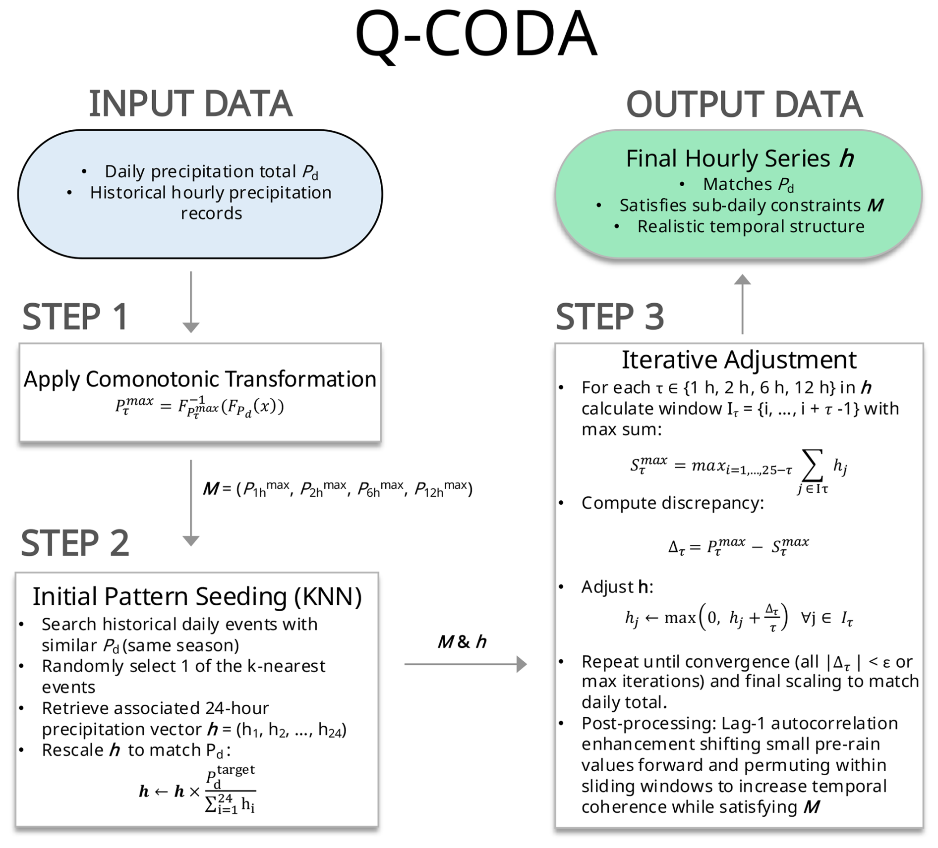
Figure 4 Flowchart summarizing the overall Q-CODA methodology. The diagram outlines the sequential steps involved in the disaggregation approach.

By integrating theoretical copula constraints with data-driven refinement, Q-CODA offers a hybrid approach that combines interpretability and realism. The method is particularly suitable for applications where the preservation of extreme sub-daily rainfall events is critical and provides a valuable contribution to the growing toolkit of high-temporal-resolution precipitation generation techniques.

4 Benchmark Methods

To evaluate the performance of the proposed Q-CODA method, we compare it against commonly used rainfall disaggregation techniques, including KNN, ANN-K, Poisson-cluster models, and MMRC. These methods represent a range of data-driven and stochastic approaches widely applied for sub-daily precipitation generation. In this study, they are used as benchmark methods to provide a reference against which the performance of Q-CODA can be assessed.

4.1 K-Nearest Neighbors (KNN)

The KNN method serves as an analog-based disaggregation approach. For each target daily precipitation value, historical days with similar daily totals are identified within the same climatological season (DJF, MAM, JJA, or SON), ensuring that the selected analogues reflect seasonal variability in rainfall dynamics. Similarity is assessed using Euclidean distance, and among the k closest matches, one historical 24 h pattern is randomly selected. This pattern is then linearly scaled to match the target daily total. No additional sub-daily structure adjustment is performed. This method represents a baseline based on seasonal similarity and direct pattern reuse, as described in Alzahrani et al. (2023), whose study shows that KNN (k=30) outperforms their multiplicative random cascade model and Hurst–Kolmogorov process-based model on a set of specific performance metrics and four locations.

4.2 Deep learning disaggregation model (ANN-K)

This method builds on the deep learning-based disaggregation framework proposed by Bhattacharyya et al. (2024), combining unsupervised clustering via K-Means with a supervised Artificial Neural Network (ANN). The key motivation for this hybrid approach is to improve model skill in differentiating between low-intensity and high-intensity rainfall events, which are often poorly represented by traditional neural networks due to their tendency to regress towards the mean or zero-inflated values.

Preprocessing is performed using K-Means clustering on triplets of consecutive daily rainfall values: $(P_{\mathrm{d}}^{(t-\mathrm{1})},P_{\mathrm{d}}^{\left(t\right)},P_{\mathrm{d}}^{(t+\mathrm{1})})$. The clustering is done in three-dimensional space to capture the temporal context around each day. The optimal number of clusters is selected using the Silhouette Coefficient method (Rousseeuw, 1987), ranging from K=2 to 9. This categorical information (cluster labels) is used as an additional input to the ANN, allowing the model to better differentiate convective events, dry days, and transitional regimes. Our model introduces an architecture comprising a 4-layer feedforward neural network, defined as follows: (i) Input layer – a concatenated vector consisting of daily rainfall and the corresponding cluster label; (ii) First hidden layer – 64 neurons with ELU (Exponential Linear Unit) activation; (iii) Second hidden layer – 32 neurons with ELU activation; and (iv) Output layer – 24 neurons (representing hourly rainfall estimates), with a linear activation function. This structure enables the model to learn abstract representations of intra-daily rainfall patterns. The use of ELU (Exponential Linear Unit) activation functions helps to reduce vanishing gradients and maintain responsiveness for negative inputs, improving convergence during training. We adopt the ELU activation function used by Bhattacharyya et al. (2024), as it provides improved numerical stability and convergence compared to ReLU and LeakyReLU for sparse and skewed precipitation data. In addition, the formulation of the loss function has a decisive influence (Lopez-Gomez et al., 2023; Oates et al., 2025) on the model's skill to disaggregate precipitation events. To guide the ANN toward physically meaningful disaggregation, we define a composite loss function that combines multiple criteria: (i) L₁ – hourly MSE: Mean squared error between predicted and observed hourly rainfall values; (ii) L₂ – error in reproducing the maximum 1 h precipitation; (iii) L₃ – convectivity penalty, defined only for days with daily total ≥20 mm and ratio between the maximum 1 h precipitation and daily total greater than 0.7, emphasizing accurate reconstruction of convective peaks; (iv) L₄ – error in hourly precipitation mean; (v) L₅ – error in hourly precipitation variance; (vi) L₆ – daily cumulative absolute error computed between predicted and observed hourly rainfall distributions. L₅ was already introduced by Oates et al. (2025), and L₆ serves the same purpose as the Kullback–Leibler divergence also used by Oates et al. (2025). Unlike Bhattacharyya et al. (2024), who used a basic MSE loss (L₁), our custom loss explicitly penalizes timing and shape errors in intense rainfall events, which are critical for flood forecasting and infrastructure design. The model was trained using the Adam optimizer (learning rate=0.001), with early stopping based on validation loss.

4.3 Poisson-Cluster Rainfall Generator

The Poisson-Cluster Disaggregation Method (PCDM) is a stochastic framework designed to disaggregate daily precipitation totals into hourly values. The method is based on a simplified Poisson cluster process (Onof et al., 2000), where storm events (or rain cells) are randomly generated within each day according to a Poisson distribution whose rate parameter is conditioned on the daily total precipitation P_d. Each storm cluster has a random start time, duration, and intensity, sampled from appropriate distributions (uniform, discrete, and gamma, respectively), and the total hourly series is scaled to match the original daily total. The number of intra-day events, N, follows a Poisson distribution with parameter $\mathit{\lambda }=(\mathrm{1.5},P_{\mathrm{d}}/D)$, where D is a station-specific scaling divisor. Each event is assigned a start time (random hour of the day), a random duration (1 to 3 h), and an intensity drawn from a gamma distribution (shape = 2, scale = station-specific parameter). Hourly intensities are then aggregated and rescaled to ensure mass conservation, i.e., the sum over 24 h equals the daily input precipitation P_d. PCDM is implemented and applied station-wise using pre-calibrated parameters, D divisor and scale of the gamma distribution, obtained via in-site iterative minimization of 1-D Wasserstein distance between observed and simulated maximum 1 h precipitation.

4.4 Multiplicative Microcanonical Random Cascade (MMRC)

Among the family of Multiplicative Microcanonical Random Cascade (MMRC) models, we selected the implementation provided by MELODIST (MEteoroLOgical observation time series DISaggregation Tool; Förster et al., 2016), as it has been successfully applied in various recent studies (Görner et al., 2021; Hasan et al., 2023; Mayer et al., 2024) and offers a balance between physical realism, probabilistic variability, and computational simplicity. The Cascade Model implemented in MELODIST offers a purely statistical yet physically consistent approach for disaggregating daily precipitation into sub-daily resolutions. Originally proposed by Olsson (1998), this MMRC has since been enhanced by subsequent studies to better preserve sub-daily rainfall characteristics while maintaining low computational complexity. The cascade model implemented in MELODIST operates through a hierarchical, stepwise disaggregation in which each level of the time series is recursively split into two subintervals of equal duration. At each level, the precipitation in a given time box is divided into two sub-boxes by assigning a pair of weights (W₁,W₂), such that $P_{i+\mathrm{1},\mathrm{1}}=W_{\mathrm{1}}\cdot P_i$ and $P_{i+\mathrm{1},\mathrm{2}}=(\mathrm{1}-W_{\mathrm{1}})\cdot P_i=W_{\mathrm{2}}\cdot P_i$ with the mass-preserving constraint $W_{\mathrm{1}}+W_{\mathrm{2}}=\mathrm{1}$. This recursive branching continues until the desired temporal resolution is reached (e.g., 1 h). For daily to hourly disaggregation, this typically involves the sequence: $\mathrm{24}\mathrm{h}\to \mathrm{12}\mathrm{h}\to \mathrm{6}\mathrm{h}\to \mathrm{3}\mathrm{h}\to \mathrm{1.5}\mathrm{h}\to \mathrm{0.75}\mathrm{h}\to \mathrm{1}\mathrm{h}$. The model distinguishes between four types of “wet” time boxes: (i) Starting box, follows a dry interval and precedes a wet one; (ii) Ending box, follows a wet interval and precedes a dry one; (iii) Isolated box, surrounded by dry intervals; and (iv) Enclosed box, surrounded by wet intervals. Each of these box types is associated with a set of probabilistic rules for assigning the weights (W₁,W₂), with three possible branching scenarios: (i) (0,1), all precipitation goes to the second subinterval; (ii) (1,0), all precipitation goes to the first subinterval; and (iii) $(x,\mathrm{1}-x)$, where precipitation is split proportionally with a random weight $x\in (\mathrm{0},\mathrm{1})$. The probabilities associated with each case are derived empirically through a reverse scaling procedure applied to high-temporal-resolution rainfall data. During this process, fine-resolution data is aggregated up the cascade (e.g., $\mathrm{1}\mathrm{h}\to \mathrm{2}\mathrm{h}\to \mathrm{4}\mathrm{h}\to \mathrm{8}\mathrm{h}$, etc.), and the branching weights and their frequencies are recorded for each box type and precipitation intensity class (above or below the mean). Instead of fitting parametric distributions, the model uses empirical histograms of weight values ($x\in [\mathrm{0},\mathrm{1}]$) divided into seven bins. These empirical distributions and associated branching probabilities are stored in lookup tables, which serve as input for a random number generator during disaggregation. For each cascade step during disaggregation, a random number is used to determine the branching type – either (0,1), (1,0), or $(x,\mathrm{1}-x)$; if the $(x,\mathrm{1}-x)$ case is selected, a second random number is drawn to choose the specific weight bin x, and the precipitation volume is then split accordingly between the two resulting time steps, ensuring that the total mass is preserved at every level. Because the process is stochastic, different disaggregation realizations may vary, though their statistical properties remain consistent by design. The MMRC model preserves key physical constraints such as precipitation volume conservation (microcanonical property) and captures the intermittency and variability of sub-daily rainfall events with minimal parameterization. The cascade algorithm is a computationally efficient and robust method for producing sub-daily rainfall inputs for hydrological modelling, especially when sub-daily observations are unavailable or sparse.

5 Evaluation Framework

To rigorously evaluate the skill and generalization capacity of the proposed Q-CODA, we implement a 5-fold cross-validation procedure (Gutiérrez et al., 2019; Hernanz et al., 2022; Gong et al., 2026) using the dataset described in Sect. 2, comprising 91 meteorological stations distributed across diverse climatic regions of Spain over the period 1996–2024. Each fold corresponds to a distinct multi-year period: Fold 1 (1996–2001), Fold 2 (2002–2007), Fold 3 (2008–2013), Fold 4 (2014–2019), and Fold 5 (2020–2024). The remaining folds are used for training, and the full period is reconstructed by aggregating the five validation folds. The performance of Q-CODA is compared against four established disaggregation methods described in Sect. 4: KNN, ANN-K, PCDM, and MMRC. All evaluations are performed independently at each station, and results are subsequently aggregated across the 91 stations for analysis and visualization.

The first part of the evaluation focuses on 1 h maximum precipitation ($P_{\mathrm{1}\mathrm{h}}^{\text{max}}$), a critical variable for hydrological simulations, risk assessment, and infrastructure design due to its direct relation to peak intensities and convective extremes. By centring the analysis on this high-impact variable, we ensure that the evaluation prioritizes features most relevant to extreme event representation. Model skill is quantified using standard accuracy metrics, Nash–Sutcliffe Efficiency (NSE) and Mean Absolute Error (MAE), calculated across the full $P_{\mathrm{1}\mathrm{h}}^{\text{max}}$ time series. In addition, distributional similarity is assessed using the first-order Wasserstein distance between observed and simulated $P_{\mathrm{1}\mathrm{h}}^{\text{max}}$ distributions. To further probe distributional fidelity, we compute relative biases (%) in the mean, variance, and upper-tail quantiles (99th, and 99.9th percentiles), and maximum value of $P_{\mathrm{1}\mathrm{h}}^{\text{max}}$. Beyond daily extremes, the second component of the evaluation addresses the temporal consistency and structural realism of the full disaggregated hourly time series. Metrics include bias in the temporal mean and temporal variance, the mean duration of precipitation events, as well as the zero proportion (the fraction of dry hours) which captures rainfall intermittency. These structural descriptors are essential for ensuring that the internal dynamics of rainfall sequences are plausible and useful for process-based modelling. Temporal correlation structure is further assessed via biases in the autocorrelation coefficients at lags of 1, 2, 6, and 12 h, providing insight into the persistence and organization of precipitation over sub-daily timescales. Finally, to assess the hydrological applicability of each method, we compare Intensity–Duration–Frequency (IDF) curves derived from disaggregated outputs to those obtained from observed hourly records. For the estimation of IDF curves, the classical annual maxima approach was adopted, which remains the standard in hydrological applications. Although alternative methods such as the peaks-over-threshold (POT) framework exist, the annual maxima method was selected to ensure comparability with previous studies, given that the primary focus of this work is the evaluation of the disaggregation algorithm. For each duration (1–24 h), annual maxima were extracted from the hourly precipitation series using a rolling sum. These maxima were fitted to a Gumbel distribution using maximum likelihood estimation. Return levels (mm) were then computed with the Gumbel inverse CDF:

$$\begin{array}{}\text{(11)}& x_T=\mathit{\mu }-\mathit{\beta }\cdot \ln [-\ln (\mathrm{1}-\mathrm{1}/T\left)\right],\end{array}$$

where μ and β are the fitted parameters and T is the return period (years). Intensities (mm h⁻¹) were obtained by dividing each estimate by its duration.

This analysis is conducted at all sites, enabling evaluation of each model's capacity to reproduce local extremes and temporal scaling behaviours under varied climatic conditions. This multi-faceted validation framework thus offers a robust basis for comparing the accuracy, distributional fidelity, and physical realism of alternative disaggregation approaches.

6 Results

This Sect. 6 presents the results of the 5-fold cross-validation, comparing the performance of Q-CODA against the state-of-the-art disaggregation methods described in Sect. 4. The aim is to highlight where Q-CODA improves upon existing approaches and to identify trade-offs across the evaluated metrics.

Figure 5 presents a comparative evaluation of the disaggregation methods based on their ability to reconstruct the daily maximum 1 h precipitation ($P_{\mathrm{1}\mathrm{h}}^{\text{max}}$) across 91 meteorological stations. Each subfigure corresponds to a different performance metric and summarizes its spatial distribution across stations through boxplots, covering accuracy, distributional similarity, and extreme value behaviour. Across all these metrics, Q-CODA consistently outperforms the methods described in Sect. 4, demonstrating superior accuracy and robustness in reproducing high-temporal-resolution rainfall extremes. In terms of MAE (Fig. 5a), Q-CODA exhibits the lowest errors across the station network, followed closely by ANN-K. The remaining methods – KNN, PCDM, and MMRC – yield significantly higher errors, with highly similar performance distributions. For the NSE (Fig. 5b), Q-CODA and ANN-K attain the highest median values, approaching 0.75, while KNN, PCDM, and MMRC display lower medians in the range of 0.5 to 0.6. Notably, MMRC exhibits a broader interquartile range and a substantially extended lower whisker, indicating greater spatial variability and underperformance at some locations. The results for the 1-D Wasserstein distance (Fig. 5c) further confirm the advantage of Q-CODA, which yields the lowest values overall, indicating the closest alignment with the observed distribution of $P_{\mathrm{1}\mathrm{h}}^{\text{max}}$. KNN ranks second, while the other methods perform markedly worse. Interestingly, ANN-K performs the worst despite its custom loss function, underscoring the limitations of neural networks in preserving distributional shapes under regression pressure. With respect to the bias in the mean (Fig. 5d), Q-CODA again leads with minimal bias, followed by KNN. In contrast, ANN-K and MMRC exhibit wide interquartile ranges, and PCDM shows a consistent negative bias. The evaluation of variance bias (Fig. 5e) highlights a major strength of Q-CODA, which substantially outperforms the alternatives. KNN and MMRC tend to overestimate variance, whereas ANN-K and PCDM show systematic underestimation, a well-documented limitation of neural network-based disaggregation (Oates et al., 2025; Bhattacharyya et al., 2024). Regarding extreme rainfall reconstruction, panels 5f through 5 h show biases in the 99th percentile, 99.9th percentile, and maximum of daily $P_{\mathrm{1}\mathrm{h}}^{\text{max}}$ values. Q-CODA delivers remarkably low biases in the 99th and 99.9th percentiles and remains the best-performing method even when evaluating the absolute maximum, despite a slight increase in error. The other methods struggle considerably with tail behaviour: ANN-K systematically underestimates extremes, MMRC tends to overestimate them, and PCDM performs similarly to ANN-K in this regard. KNN offers moderately accurate results but falls short of Q-CODA. The poor performance of ANN-K in reproducing maximum $P_{\mathrm{1}\mathrm{h}}^{\text{max}}$ may also stem from the well-known limitation of deep learning models to extrapolate beyond the range of their training data.

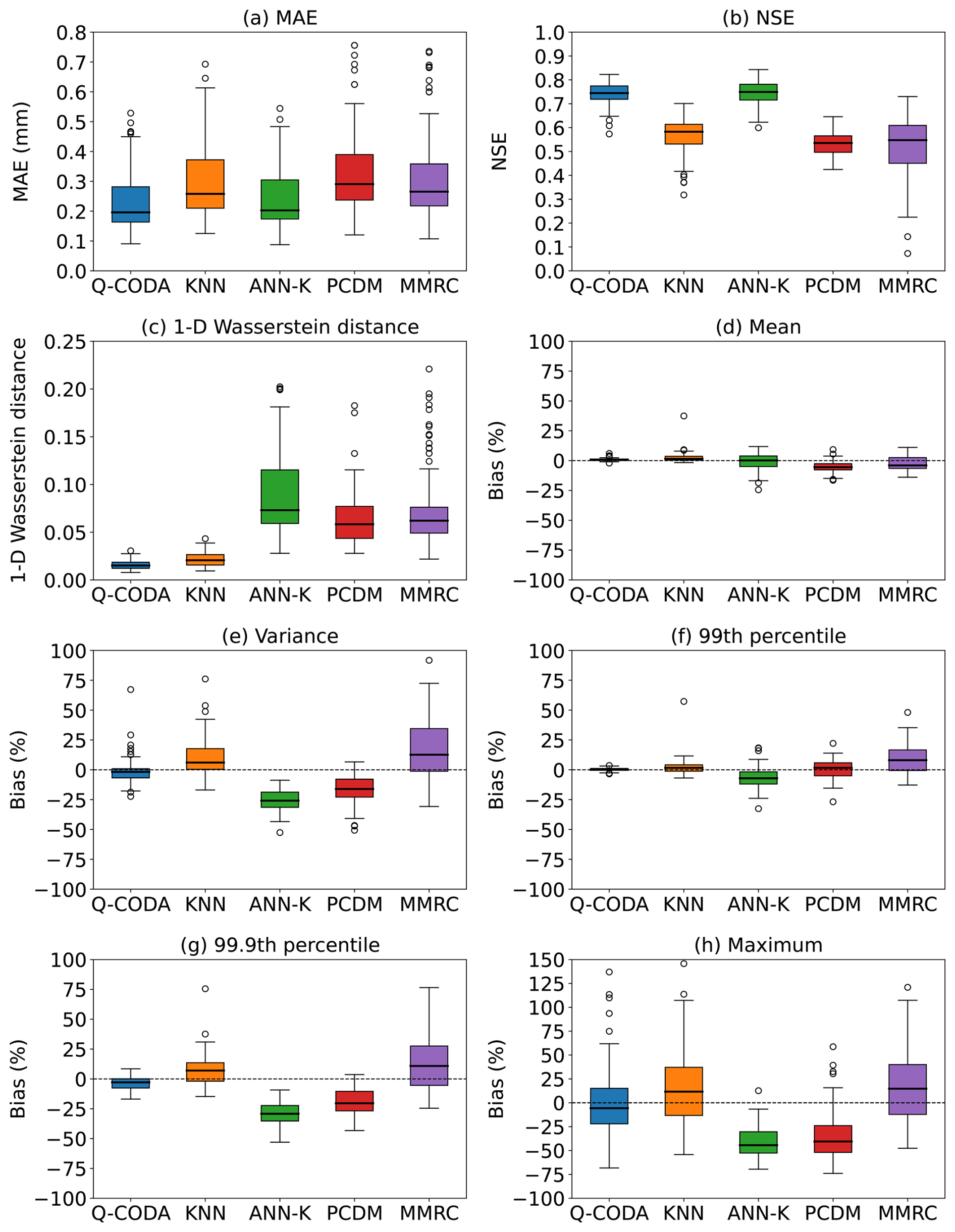
Figure 5 Comparative evaluation of disaggregation methods based on their ability to reconstruct daily maximum 1 h precipitation ($P_{\mathrm{1}\mathrm{h}}^{\text{max}}$) across 91 meteorological stations. Each panel shows boxplots summarizing the spatial distribution of key performance metrics: (a) Mean Absolute Error (MAE), (b) Nash–Sutcliffe Efficiency (NSE), (c) 1-D Wasserstein distance, (d) bias in the mean, (e) bias in the variance, (f) bias in the 99th percentile, (g) bias in the 99.9th percentile, and (h) bias in the maximum.

Overall, the results in Fig. 5 demonstrate the superior ability of Q-CODA to reproduce both the magnitude and statistical characteristics of peak sub-daily precipitation. Its consistent performance across multiple metrics and spatial locations highlights its value as a disaggregation tool that reliably reproduces observed rainfall features.

Figure 6 presents a comparative assessment of the disaggregation methods based on their ability to reproduce key statistical and temporal properties of the full hourly time series at the 91 evaluation stations. Each subplot shows the spatial distribution of bias (%) for different metrics, summarized through boxplots, where each box reflects variability across sites. The analysed metrics include bias in the temporal mean and variance, zero proportion, mean event duration, and autocorrelation at multiple time lags. For the mean of the hourly series (Fig. 6a), Q-CODA exhibits an almost negligible bias, clearly outperforming the other methods. KNN, PCDM, and MMRC follow with slight underestimations, while ANN-K stands out negatively, displaying a more pronounced underestimation close to 0.5 %. The results for the variance (Fig. 6b) show a similar pattern. Q-CODA again achieves the lowest bias, followed by KNN, PCDM, and MMRC, which tend to modestly underestimate variability. ANN-K shows the most significant underestimation, with a median bias exceeding 25 %, confirming the well-known difficulty of neural networks in reproducing precipitation variability, as previously documented by Bhattacharyya et al. (2024) and Oates et al. (2025). When evaluating the proportion of zero values (Fig. 6c), which corresponds to the share of dry hours, KNN achieves the lowest bias, followed closely by Q-CODA and MMRC. ANN-K and PCDM show worse performance, with ANN-K underestimating and PCDM overestimating the frequency of dry periods. For the mean event duration (Fig. 6d), Q-CODA again demonstrates the best performance, yielding the smallest bias across stations. KNN and PCDM both tend to underestimate event lengths, while MMRC shows a tendency to overestimate. ANN-K has its median bias near zero, but a large interquartile range indicates high spatial variability and reduced robustness. Autocorrelation results further highlight Q-CODA's superiority. Across all autocorrelation lags (Fig. 6e–h), Q-CODA consistently exhibits the lowest median bias. While MMRC shows the smallest median bias at lag-12, Q-CODA achieves a narrower interquartile range, suggesting greater spatial consistency. KNN systematically underestimates autocorrelation across all lags. PCDM and MMRC also show underestimation, except for lag-12 where MMRC slightly improves. The issue of autocorrelation underestimation in the MMRC approach had previously been identified and reported by Müller and Haberlandt (2018). ANN-K transitions from underestimation at lag-1, to a nearly unbiased result at lag-2, but then shifts to strong overestimation at lag-6 and lag-12, pointing to instability in its representation of temporal structure.

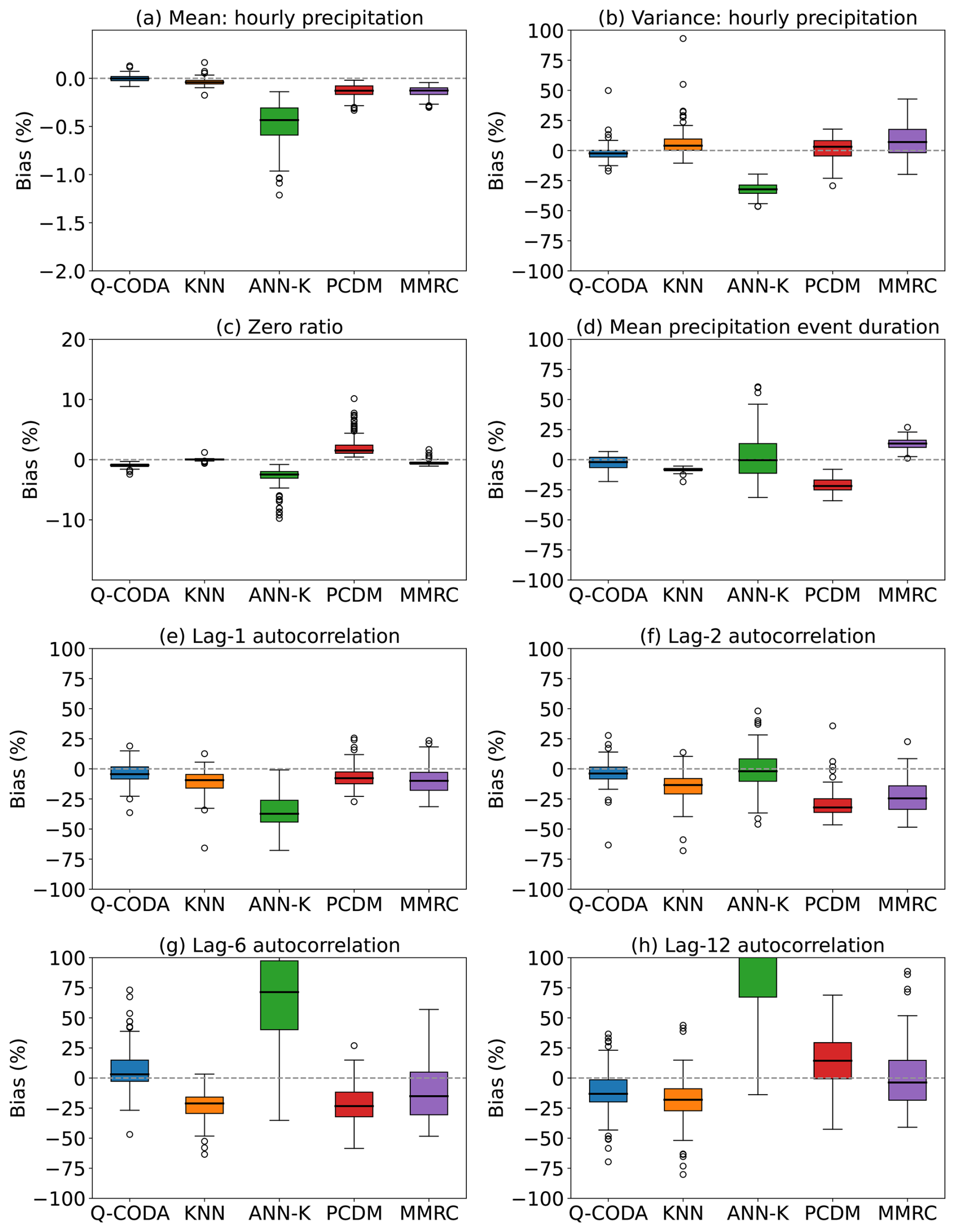
Figure 6 Comparative evaluation of disaggregation methods based on their ability to reconstruct complete hourly precipitation time series across 91 meteorological stations. The panel presents boxplots summarizing the spatial distribution of key performance metrics: (a) mean hourly precipitation, (b) hourly precipitation variance, (c) bias in zero proportion, (d) bias in mean precipitation event duration, (e) bias in lag-1 autocorrelation, (f) bias in lag-2 autocorrelation, (g) bias in lag-6 autocorrelation, and (h) bias in lag-12 autocorrelation.

Similarly, the metrics in Fig. 6 show that Q-CODA achieves the best or near-best performance across all statistical and temporal features of the hourly rainfall series, providing a consistent advantage over state-of-the-art methods.

The realistic reproduction of key temporal rainfall characteristics, such as the proportion of zero values, the mean precipitation event duration, and the autocorrelation structure, is critical in hydrological applications, as these attributes directly influence runoff generation, soil moisture dynamics, and flood modelling. An over- or underestimation of dry intervals (i.e., zero proportion) can distort the temporal distribution of rainfall, while inaccuracies in event duration may lead to erroneous estimates of infiltration and surface flow. Similarly, the autocorrelation of rainfall, particularly at short lags, affects the temporal persistence of wet conditions, which in turn shapes hydrological responses at various scales. Among the evaluated disaggregation methods, Q-CODA stands out by most accurately preserving these features across the network of stations. Its ability to replicate the observed structure of rainfall time series with high fidelity enhances the reliability of downstream hydrological simulations, making it a robust tool for both historical analysis and future climate impact assessments.

To evaluate the ability of each disaggregation method to reproduce observed IDF (Intensity–Duration–Frequency) relationships, we conducted an illustrative case study at the Reus station (41.1450° N, 1.1636° E), which lies within a Mediterranean climate zone (Köppen–Geiger climate classification Csa). This site was selected because it exhibits one of the highest recorded 1 h precipitation among all stations in the historical dataset. Figure 7 compares the IDF curves obtained from each method against the observed benchmark for return periods of 2, 5, 10, 25, 50, and 100 years. Q-CODA closely tracks the empirical IDF across all return periods, exhibiting minimal deviation even at more extreme thresholds. MMRC also performs well in this case, yielding simulated IDF curves that remain relatively consistent with the observations. By contrast, the IDF curves produced by KNN, ANN-K, and PCDM deviate more substantially from the reference, especially at longer return periods. While informative, this example represents a single location and does not capture the broader spatial variability in IDF performance. To address this, we computed the root mean squared error (RMSE) between simulated and observed IDF curves at each station and for each method, yielding a spatial distribution of RMSE values summarized via boxplots in Fig. 8. This analysis reveals that Q-CODA consistently achieves the lowest IDF reconstruction error across the network of 91 stations, followed (at increasing distances) by KNN, MMRC, PCDM, and ANN-K. This ranking remains stable across all return periods, although RMSE values increase with return period, reflecting the greater challenge of accurately modelling rare extremes. These results underscore Q-CODA's superior capacity to preserve high-order rainfall statistics essential for hydrological design and risk assessment.

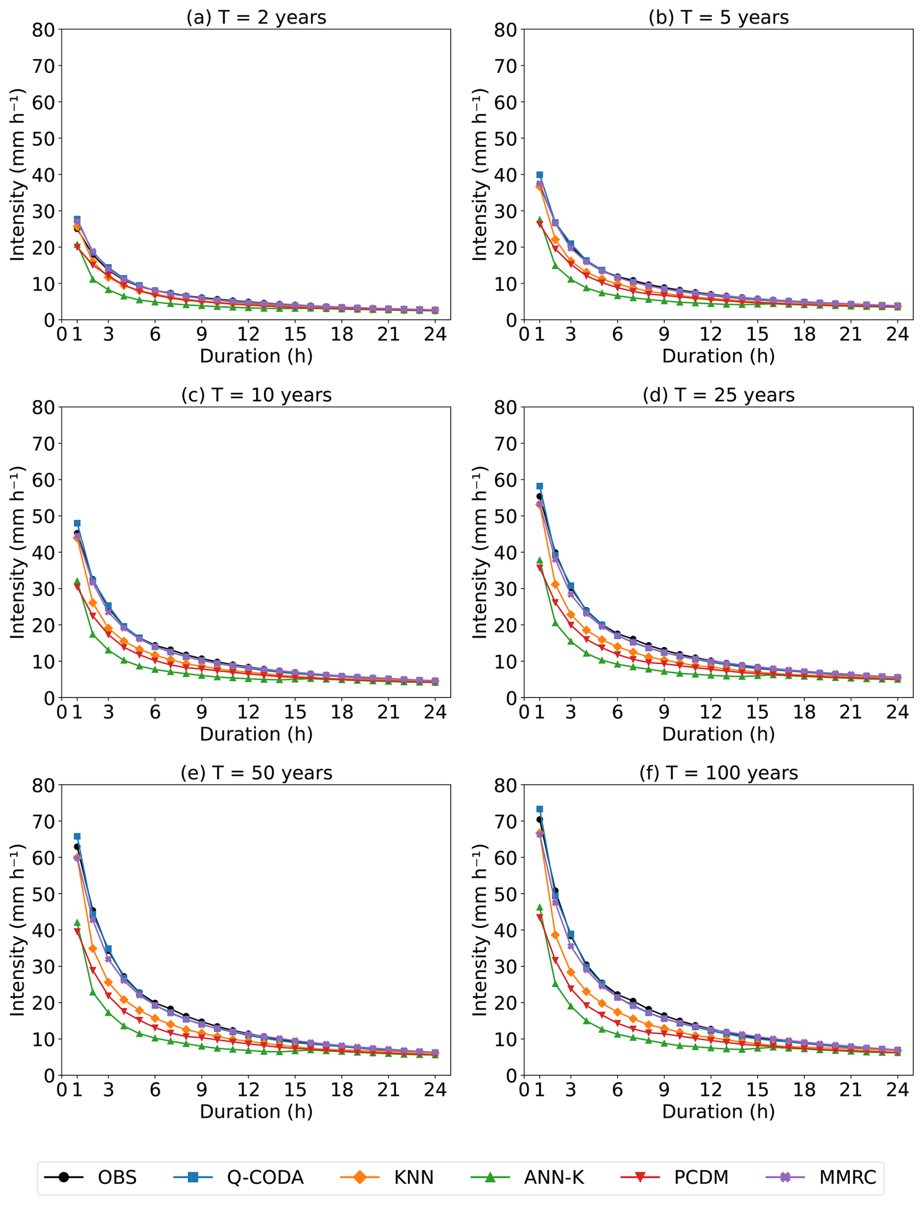
Figure 7 Comparison of Intensity–Duration–Frequency (IDF) curves derived from each disaggregation method with the observed benchmark at the Reus station (41.1450° N, 1.1636° E). Curves are shown for return periods of 2, 5, 10, 25, 50, and 100 years.

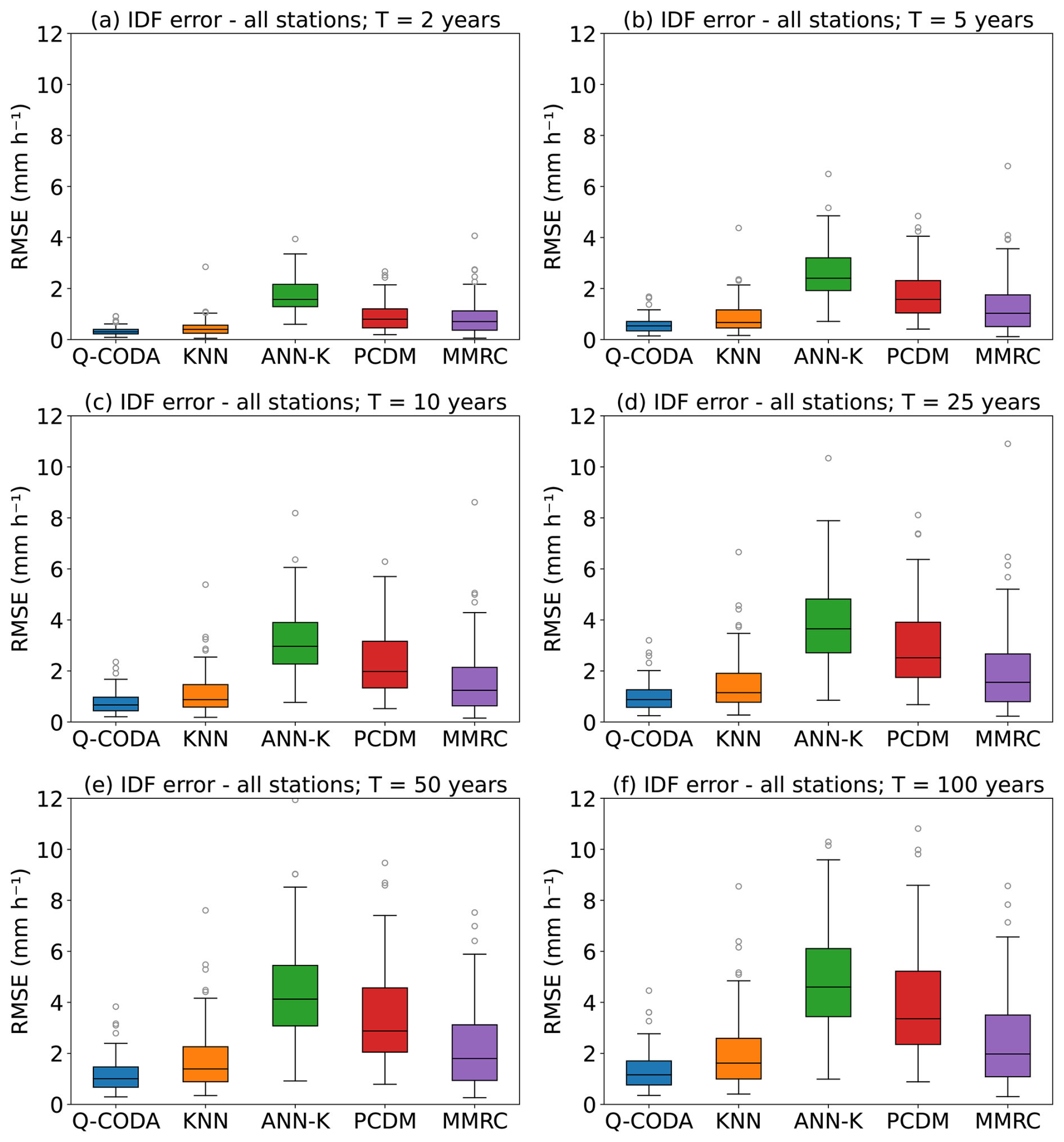
Figure 8 Spatial distribution of root mean squared error (RMSE) between observed and simulated IDF (Intensity–Duration–Frequency) curves across 91 meteorological stations, grouped by disaggregation method. Boxplots summarize the performance variability of each method in reproducing IDF relationships, providing a broader evaluation beyond the single-station case study shown in Fig. 7.

To further assess the practical applicability of the proposed framework, the computational efficiency of Q-CODA was evaluated in comparison with the benchmark methods. Given its iterative structure, particular attention was paid to runtime and computational footprint. A comparative experiment was conducted using all methods on the same reference station employed for the derivation of the IDF curves (Fig. 7), ensuring consistent input data and processing conditions. All computations were performed on a workstation equipped with an Intel Xeon Gold 5218 processor (32 cores) and 63 GB of RAM, and computational cost and energy consumption were estimated using the CodeCarbon library (Courty et al., 2026). Overall, the results (see Table 1) indicate that, although Q-CODA entails a higher computational demand than some state-of-the-art approaches, execution times remain within practical limits for offline applications. Furthermore, the structure of the algorithm allows for parallelization, offering clear potential for reducing runtime in large-scale or operational contexts. These findings support the computational feasibility of Q-CODA and provide additional context for its application in scenarios requiring accurate disaggregation under diverse hydroclimatic conditions.

Table 1 Comparison of computational costs across methods.

7 Discussion

7.1 Performance variability across stations

While Q-CODA generally performs consistently across the 91 evaluation AEMET stations, some isolated outliers are observed in specific metrics (e.g. variance bias and lag-2 autocorrelation bias of the reconstructed hourly series, in Fig. 6b and f, respectively). To assess whether these outliers are linked to station-specific characteristics or to weaker quasi-comonotonic dependence between daily totals and sub-daily maxima, we conducted an additional diagnostic analysis. The results indicate that the outliers are not driven by persistent station-level data quality issues. Instead, the variability appears to be method- and metric-dependent. Sect. S4 in the Supplement provides a detailed investigation of these aspects.

7.2 Applicability to other climatic regimes

The performance of Q-CODA relies on empirical quasi-comonotonicity, which may exhibit different validity across precipitation regimes. To assess the robustness of the method under heterogeneous climatic conditions, we extend the evaluation by stratifying the 91 AEMET stations used in Sect. 6 according to regional climatic characteristics. Specifically, stations are grouped into Mediterranean and southern, inland, and northern/northwestern regimes. For each subgroup, we analyse the distributional agreement between observed and disaggregated daily maximum 1 h precipitation using Q–Q plots (Fig. 9). These diagnostics are computed consistently across all disaggregation methods included in the comparison, enabling a direct assessment of regime-dependent performance differences. The results provide a comparative view of method behaviour across climatic settings, highlighting differences in how well each approach reproduces the upper tail of the hourly precipitation distribution under varying regional conditions. In particular, Q-CODA shows consistently improved agreement across all subgroups, indicating a more stable performance across climatic regimes.

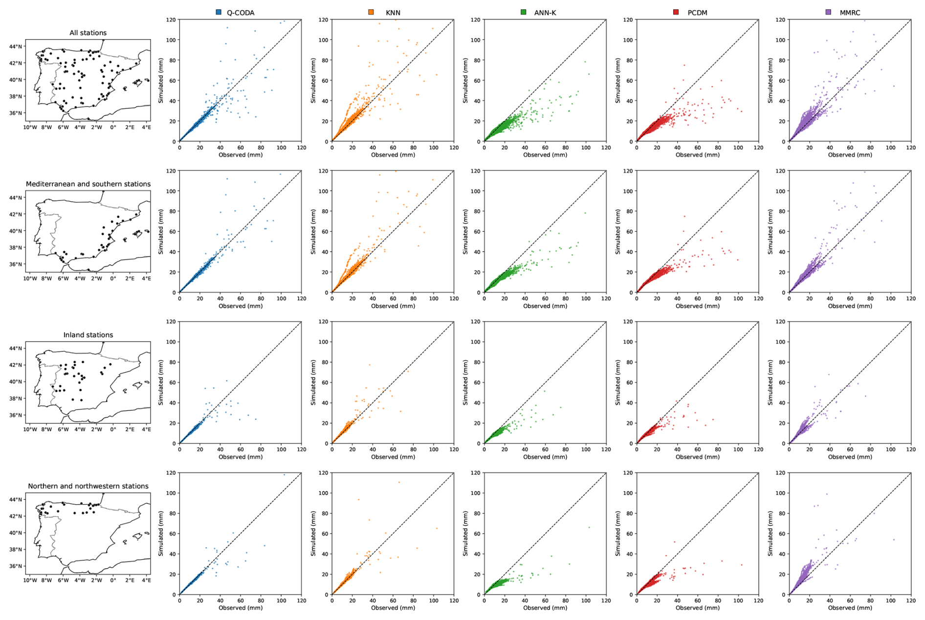
Figure 9 Q–Q plots of observed versus simulated daily maximum 1 h precipitation for the evaluated disaggregation methods across different station groups in Spain (all stations, Mediterranean and southern, inland, and northern and northwestern regions).

This regional analysis based on AEMET stations provides an initial assessment of the method's versatility across different climatic settings. In the following part of this Sect. 7.2, we extend the evaluation to independent observational datasets from the NCEI/NOAA network (Wuertz et al., 2018), focusing on contrasting climatic regimes such as the Pacific Northwest (mid-latitude oceanic climate with long-duration frontal precipitation) and Florida (tropical monsoon environment with intense convective rainfall), in order to further explore the applicability of the proposed approach under markedly different precipitation regimes. Because publicly available long-term hourly precipitation datasets with consistent coverage are limited, we focused on stations from the NCEI/NOAA archive where sufficiently long records exist. Note that reanalysis products are generally unable to adequately capture precipitation extremes unless they are generated with convection-permitting resolutions, as coarse-grid configurations tend to smooth or underestimate short-lived, high-intensity convective events; for this reason, they were not considered in the present study.

We first analysed five stations in the Pacific Northwest of the United States (Köppen Cfb climate), a region characterized by persistent frontal systems and prolonged moderate rainfall. The selected stations include three located on the Olympic Peninsula in Washington State (COOP:450013, COOP:456114, COOP:456624) and two coastal stations in Alaska (COOP:500352, COOP:509941). The geographical distribution of these stations is shown in Fig. S4 in the Supplement. These stations are characterized by long-duration frontal precipitation systems and persistent moderate rainfall. For these locations, we computed the Spearman correlation between daily totals and sub-daily maxima ${\mathit{\rho }}_{\mathrm{S}}(P_{\mathrm{1}\mathrm{h}}^{\text{max}},P_{\mathrm{d}})$ and evaluated the same performance metrics used in the main study (Wasserstein distance for the $P_{\mathrm{1}\mathrm{h}}^{\text{max}}$ distribution, bias in the 99.9th percentile, lagged autocorrelation bias, and IDF-based RMSE). For consistency with the Spanish case study while accounting for data availability in the NCEI/NOAA archive, the evaluation period for the international stations was extended to 50 years (1951–2000). The same validation framework was applied using a 5-fold cross-validation scheme, where each fold corresponds to a continuous 10-year block. This configuration ensures temporal robustness in the assessment while maximizing the use of the available long-term hourly precipitation records.

The results (see Fig. 10) show that the quasi-comonotonic relationship remains strong even in this more persistent rainfall regime, although slightly weaker than in Spain. The lowest observed Spearman correlation decreases to approximately 0.984, whereas in the Spanish dataset even the weakest stations rarely fell below 0.990. Despite this reduction, Q-CODA continues to perform robustly and consistently better than the state-of-the-art methods, particularly for extreme-value reproduction. This is reflected in the low bias in the 99.9th percentile of hourly maxima and the low RMSE in the IDF curves for a 100-year return period. These results suggest that the method remains applicable even when the quasi-comonotonicity assumption is somewhat weaker than in Mediterranean-type regimes.

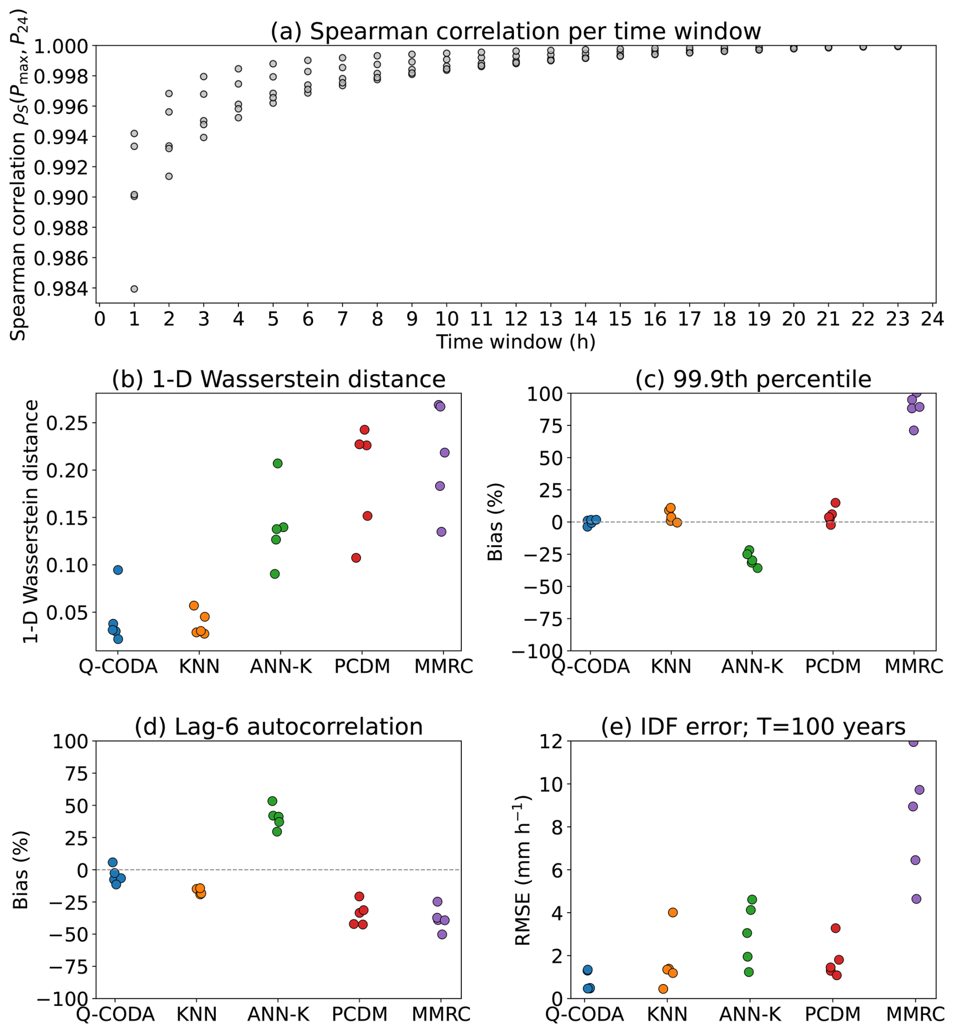
Figure 10 Performance of Q-CODA and state-of-the-art disaggregation methods (KNN, ANN-K, PCDM, and MMRC) for the five Pacific Northwest stations (Köppen Cfb). Panel (a) shows the Spearman correlation between sub-daily maxima (for different aggregation windows) and daily totals. Panels (b–e) present the evaluation metrics for the simulated series: (b) 1-D Wasserstein distance for $P_{\mathrm{1}\mathrm{h}}^{\text{max}}$, (c) bias of the 99.9th percentile of $P_{\mathrm{1}\mathrm{h}}^{\text{max}}$, (d) bias in lag-6 autocorrelation of the complete hourly series, and (e) RMSE of the IDF curves for a 100-year return period.

We also analysed three stations located in the Florida Peninsula (COOP:085663, COOP:086323, COOP:088780), representative of a tropical monsoon climate (Köppen Am), where short-lived convective bursts could in principle weaken the dependence between daily totals and sub-daily maxima. The location of these stations can be consulted in Fig. S5 in the Supplement. However, in these stations the Spearman correlation between daily totals and 1 h maxima exceeds 0.998 (see Fig. 11), which falls well within and even at the upper end of the range observed across AEMET stations in Spain. This indicates that, despite the tropical monsoonal regime and the presence of intense convective rainfall, the empirical dependence between daily accumulation and sub-daily extremes remains strongly quasi-comonotonic. Under these conditions, Q-CODA again exhibits performance fully consistent with the results reported in Sect. 6. In particular, it maintains very low bias in the 99.9th percentile of the 1 h maxima distribution and low RMSE in the 100-year IDF estimates, confirming its ability to accurately reproduce high-end extremes. At the same time, the method preserves the temporal structure of the hourly series, as reflected by stable autocorrelation. Overall, the Florida case study reinforces that when quasi-comonotonicity is strong, even in highly convective tropical environments, Q-CODA provides clear advantages over the state-of-the-art disaggregation methods.

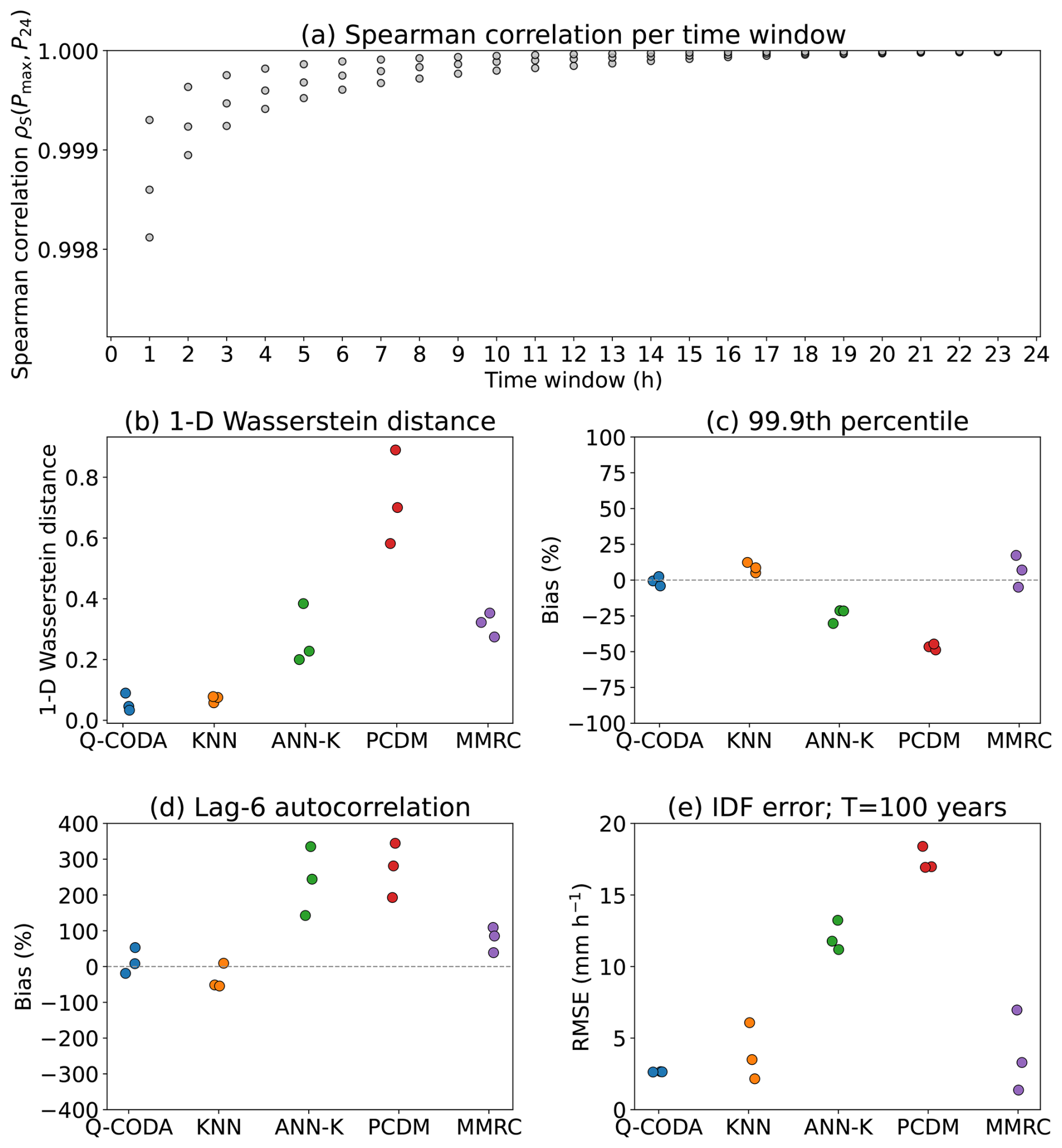
Figure 11 Performance of Q-CODA and state-of-the-art disaggregation methods (KNN, ANN-K, PCDM, and MMRC) for the three Florida stations located in a tropical monsoon climate (Köppen Am). Panel (a) shows the Spearman correlation between sub-daily maxima (for different aggregation windows) and daily totals. Panels (b–e) present the evaluation metrics for the simulated series: (b) 1-D Wasserstein distance for $P_{\mathrm{1}\mathrm{h}}^{\text{max}}$, (c) bias of the 99.9th percentile of $P_{\mathrm{1}\mathrm{h}}^{\text{max}}$, (d) bias in lag-6 autocorrelation of the complete hourly series, and (e) RMSE of the IDF curves for a 100-year return period.

Taken together, these results suggest that empirical quasi-comonotonicity is not restricted to Mediterranean-type climates, but also holds across mid-latitude oceanic and tropical monsoon regimes, albeit with varying intensity. Across all analysed cases, Q-CODA remains consistently sound and outperforms state-of-the-art approaches, particularly in the reproduction of extreme hourly precipitation. Q-CODA maintains good performance even when this observed quasi-comonotonicity dependence weakens moderately (e.g., Spearman≈0.980–0.990), as observed in the Pacific Northwest.

7.3 Sensitivity to deviations from quasi-comonotonicity

To more directly address the question regarding sensitivity to the assumption itself, we performed an additional set of controlled experiments using 15 artificial hourly precipitation series designed to emulate regimes with progressively weaker dependence between daily totals and hourly maxima. These artifitial series allow us to systematically explore conditions that are rarely observed in real long-term station records. An analysis analogous to the observational cases discussed in Sect. 7.2 was conducted, relating model performance to the Spearman correlation between daily totals and $P_{\mathrm{1}\mathrm{h}}^{\text{max}}$. The results indicate that Q-CODA remains applicable over a wide range of dependence strengths. However, when the Spearman correlation drops below approximately 0.975 (see Fig. 12), a slight degradation in performance begins to appear across metrics such as 99.9th percentile bias (Fig. 12c) and RMSE of the IDF curves (Fig. 12e), but more pronounced in the latter. In this regime, the quasi-comonotonicity assumption becomes less reliable, and the added value of the copula-based adjustment diminishes. In such hypothetical cases, the simpler KNN-based disaggregation can become preferable. In any case, Q-CODA continues to outperform ANN-K, PCDM, and MMRC.

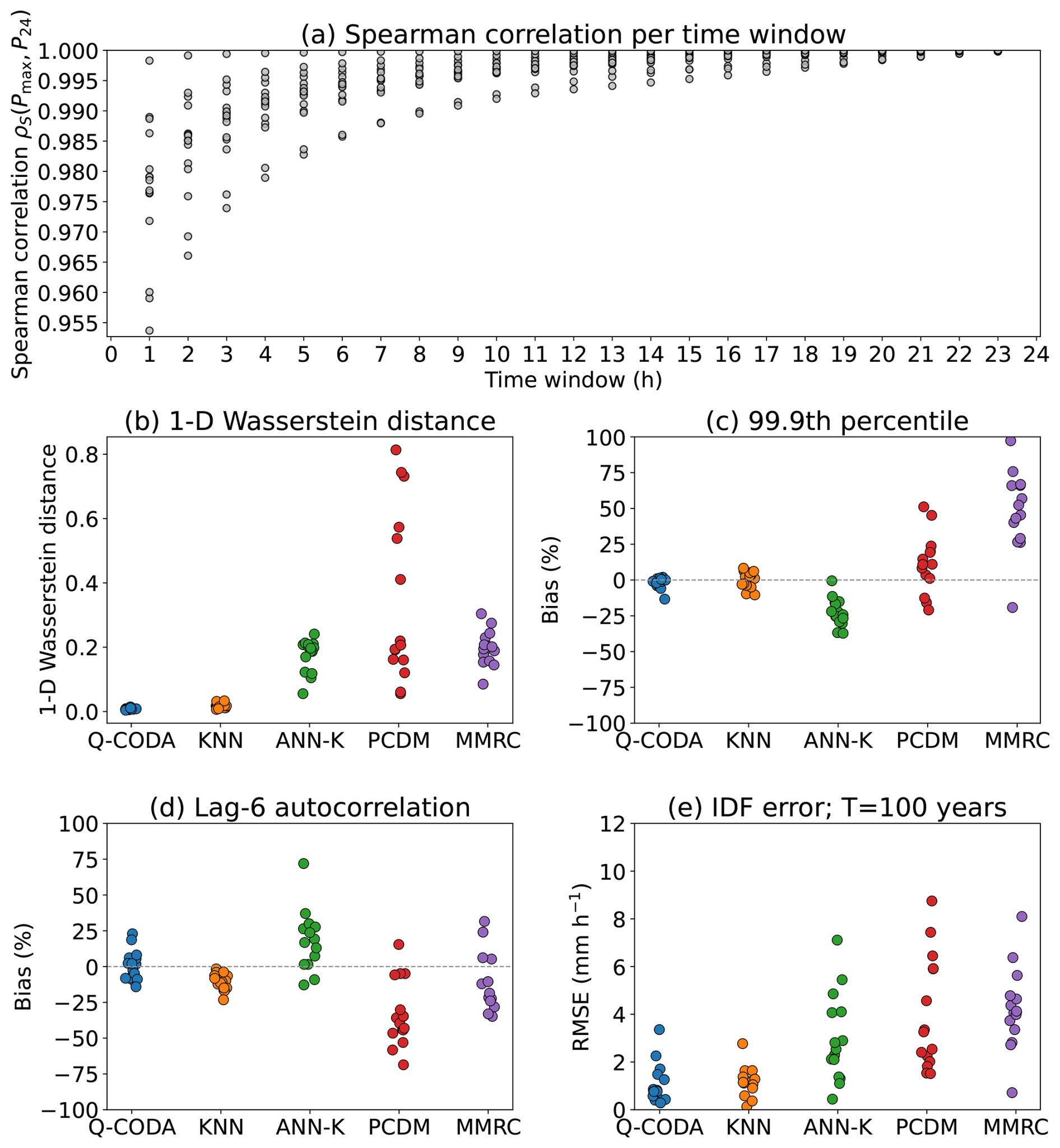
Figure 12 Performance of Q-CODA and state-of-the-art methods on 15 artificial hourly precipitation series constructed to progressively weaken the quasi-comonotonic relationship between daily totals and 1 h maxima ($P_{\mathrm{1}\mathrm{h}}^{\text{max}}$). Panel (a) shows the Spearman correlation between sub-daily maxima (for different aggregation windows) and daily totals. Panels (b)–(e) present the evaluation metrics for the simulated series: (b) 1-D Wasserstein distance for $P_{\mathrm{1}\mathrm{h}}^{\text{max}}$, (c) bias of the 99.9th percentile of $P_{\mathrm{1}\mathrm{h}}^{\text{max}}$, (d) bias in lag-6 autocorrelation of the complete hourly series, and (e) RMSE of the IDF curves for a 100-year return period.

Results indicate that Q-CODA remains consistent for moderately reduced quasi-comonotonicity dependence, but a slight degradation in performance begins to emerge when the Spearman correlation falls below approximately 0.975, providing an empirical threshold for the practical validity of the quasi-comonotonicity assumption. This threshold-based behaviour is consistent with the theoretical role of the Fréchet–Hoeffding upper bound in the method: the stronger the rank dependence between daily totals and sub-daily maxima, the more informative the percentile mapping becomes, and the more effectively Q-CODA can constrain the hourly reconstruction. Overall, sensitivity experiments suggest that the method begins to lose its advantage when the dependence drops below approximately 0.975, providing a practical guideline for assessing applicability in new regions.

7.4 Spatial component

Given that Q-CODA is based on empirical distributions, its direct applicability to ungauged or unobserved locations is limited. To address this limitation, the method has been extended to a semi-parametric regionalised framework, hereafter referred to as Q-CODA-R (Q-CODA-Regionalised). In this formulation, the purely empirical cumulative distribution functions (CDFs) used in the comonotonic transformation are replaced by seasonal Bernoulli–Gamma parametric CDFs. These distributions are fitted independently for each station, season, and accumulation duration (1, 2, 6, 12, and 24 h). The resulting distribution parameters are then spatially regionalised through universal kriging using spherical variogram models, with longitude, latitude, and elevation incorporated as external predictors. Formally, for each station, season, and accumulation duration τ (with τ=1, 2, 6, 12, 24 h), precipitation maxima is modelled using a mixed Bernoulli–Gamma distribution. Let $P_{\mathit{\tau }}^{\text{max}}$ denote the precipitation amount associated with duration τ for a given season. Its probability distribution is represented as

$$\begin{array}{}\text{(12)}& \begin{array}{rl}& Pr(P_{\mathit{\tau }}^{\text{max}}=\mathrm{0})=p_{\mathrm{0},\mathit{\tau }}\\ & Pr(P_{\mathit{\tau }}^{\text{max}}>\mathrm{0})=\mathrm{1}-p_{\mathrm{0},\mathit{\tau }}\end{array}\end{array}$$

and, conditional on $P_{\mathit{\tau }}^{\text{max}}>\mathrm{0}$,

$$\begin{array}{}\text{(13)}& P_{\mathit{\tau }}^{\text{max}}|P_{\mathit{\tau }}^{\text{max}}>\mathrm{0}\sim \text{Gamma}({\mathit{\alpha }}_{\mathit{\tau }},{\mathit{\theta }}_{\mathit{\tau }}).\end{array}$$

Where p_0,τ is the probability mass at zero precipitation, α_τ is the Gamma shape parameter, and θ_τ is the Gamma scale parameter. The parameters are estimated independently for each station and season from the observed daily maxima series for each accumulation duration. Specifically, p_0,τ is estimated as the empirical proportion of zero values,

$$\begin{array}{}\text{(14)}& p_{\mathrm{0},\mathit{\tau }}={\displaystyle \frac{\mathrm{1}}{n}}{\sum }_{i=\mathrm{1}}^n\mathbf{1}(P_{\mathit{\tau },i}^{\text{max}}=\mathrm{0}).\end{array}$$

Where n is the number of available observations and 1(⋅) is the indicator function. The Gamma parameters (α_τ, θ_τ) are then fitted by maximum likelihood using only the strictly positive observations $\mathit{\{}{P}_{\mathit{\tau },i}^{\text{max}}:P_{\mathit{\tau },i}^{\text{max}}>\mathrm{0}\mathit{\}}$, with the location parameter fixed at zero.

The resulting CDF for duration τ is therefore

$$\begin{array}{}\text{(15)}& F_{P_{\mathit{\tau }}^{\text{max}}}\left(x\right)=\left\{\begin{array}{ll}\mathrm{0},& x<\mathrm{0}\\ p_{\mathrm{0},\mathit{\tau }},& x=\mathrm{0}\\ p_{\mathrm{0},\mathit{\tau }}+(\mathrm{1}-p_{\mathrm{0},\mathit{\tau }})G(x;{\mathit{\alpha }}_{\mathit{\tau }},{\mathit{\theta }}_{\mathit{\tau }}),& x>\mathrm{0}\end{array}\right..\end{array}$$

Where $G(x;{\mathit{\alpha }}_{\mathit{\tau }},{\mathit{\theta }}_{\mathit{\tau }})$ denotes the Gamma CDF with shape α_τ and scale θ_τ.

$$\begin{array}{}\text{(16)}& \begin{array}{rl}& G(x;{\mathit{\alpha }}_{\mathit{\tau }},{\mathit{\theta }}_{\mathit{\tau }})={\displaystyle \frac{\mathrm{1}}{\mathrm{\Gamma }\left({\mathit{\alpha }}_{\mathit{\tau }}\right)}}\cdot {\displaystyle \frac{\mathrm{1}}{{\mathit{\theta }}_{\mathit{\tau }}^{{\mathit{\alpha }}_{\mathit{\tau }}}}}{\int }_{\mathrm{0}}^x{u}^{{\mathit{\alpha }}_{\mathit{\tau }}-\mathrm{1}}{e}^{-\frac{u}{{\mathit{\theta }}_{\mathit{\tau }}}}\mathrm{d}u\\ & \mathrm{\Gamma }\left({\mathit{\alpha }}_{\mathit{\tau }}\right)={\int }_{\mathrm{0}}^{\mathrm{\infty }}{t}^{{\mathit{\alpha }}_{\mathit{\tau }}-\mathrm{1}}{e}^{-t}\mathrm{d}t.\end{array}\end{array}$$

The Gamma CDF parameters are estimated numerically using SciPy (scipy.stats.gamma.fit, with floc = 0) library developed by Virtanen et al. (2020).

After fitting these parameters at station level, the spatial fields of parameters p_0,τ, α_τ, and θ_τ are regionalised by universal kriging using PyKrige (Murphy et al., 2025). For any ungauged target location s, this yields interpolated parameter estimates ${\widehat{p}}_{\mathrm{0},\mathit{\tau }}\left(s\right)$, ${\widehat{\mathit{\alpha }}}_{\mathit{\tau }}\left(s\right)$, and ${\widehat{\mathit{\theta }}}_{\mathit{\tau }}\left(s\right)$, from which a location-specific parametric CDF can be reconstructed as:

$$\begin{array}{}\text{(17)}& \begin{array}{rl}& {\widehat{F}}_{P_{\mathit{\tau }}^{\text{max}}}(x;s)=\\ & \left\{\begin{array}{ll}\mathrm{0},& x<\mathrm{0}\\ {\widehat{p}}_{\mathrm{0},\mathit{\tau }}\left(s\right),& x=\mathrm{0}\\ {\widehat{p}}_{\mathrm{0},\mathit{\tau }}\left(s\right)+(\mathrm{1}-{\widehat{p}}_{\mathrm{0},\mathit{\tau }}(s\left)\right)G(x;{\widehat{\mathit{\alpha }}}_{\mathit{\tau }}(s),{\widehat{\mathit{\theta }}}_{\mathit{\tau }}(s\left)\right),& x>\mathrm{0}\end{array}\right..\end{array}\end{array}$$

This reconstructed seasonal and duration-specific CDF is the one subsequently used within the comonotonic transformation step of Q-CODA-R. In practice, for a given daily precipitation total P_d, the corresponding non-exceedance probability is first obtained from the kriged 24 h distribution,

$$\begin{array}{}\text{(18)}& q={\widehat{F}}_{P_{\mathrm{d}}}(P_{\mathrm{d}};s)\equiv {\widehat{F}}_{P_{\mathrm{24}}}(P_{\mathrm{24}};s).\end{array}$$

For τ<24, the target sub-daily maxima are obtained by applying the same non-exceedance probability q to the corresponding mixed Bernoulli–Gamma distribution. If $q<{\widehat{p}}_{\mathrm{0},\mathit{\tau }}\left(s\right)$, then ${\widehat{P}}_{\mathit{\tau }}^{\text{max}}=\mathrm{0}$; otherwise, the conditional Gamma quantile is computed as:

$$\begin{array}{}\text{(19)}& q_{\mathit{\tau }}^{\ast }={\displaystyle \frac{q-{\widehat{p}}_{\mathrm{0},\mathit{\tau }}\left(s\right)}{\mathrm{1}-{\widehat{p}}_{\mathrm{0},\mathit{\tau }}\left(s\right)}},\end{array}$$

and this same probability level is then comonotonically transferred to the shorter durations through the inverse CDFs using SciPy (scipy.stats.gamma.ppf):

$$\begin{array}{}\text{(20)}& {\widehat{P}}_{\mathit{\tau }}^{\text{max}}=G^{-\mathrm{1}}(q_{\mathit{\tau }}^{\ast };{\widehat{\mathit{\alpha }}}_{\mathit{\tau }}(s),{\widehat{\mathit{\theta }}}_{\mathit{\tau }}(s\left)\right);\mathit{\tau }\in \mathit{\{}\mathrm{1},\mathrm{2},\mathrm{6},\mathrm{12}\mathit{\}}.\end{array}$$

It is equivalent to:

$$\begin{array}{}\text{(21)}& {\widehat{P}}_{\mathit{\tau }}^{\text{max}}={\widehat{F}}_{P_{\mathit{\tau }}^{\text{max}}}^{-\mathrm{1}}(q;s);\mathit{\tau }\in \mathit{\{}\mathrm{1},\mathrm{2},\mathrm{6},\mathrm{12}\mathit{\}},\end{array}$$

thus preserving the comonotonic dependence structure between the daily total and the sub-daily maxima while allowing the transformation to be applied at locations without local hourly training data.

To evaluate whether this extension truly enables application at unobserved locations, we designed a strict leave-one-station-out (LOSO) experiment over the 91 AEMET stations used in the benchmark comparison (all with >90 % completeness) in Sect. 6. Importantly, for each target station, the regionalised method was applied without using any data from that station itself. Instead: (1) the parametric CDFs were reconstructed from kriged Bernoulli–Gamma parameters, and (2) the KNN seed day used to reconstruct the intra-daily temporal structure was taken from the geographically nearest station, rather than from the target station. This second component is precisely what makes Q-CODA-R a semi-parametric, rather than a fully parametric, regionalised framework, since the seed-day still relies on an empirical K-nearest-neighbour analogue rather than on a fully parameterised stochastic model.

To improve the spatial support of the regionalisation step, the kriging models were fitted using a larger set of stations with at least 35 % completeness over 1996–2024 (approximately ≥10 years of hourly observations). This broader network was used only to estimate the spatial structure of the distribution parameters, while the actual performance evaluation remained restricted to the independent set of 91 high-quality evaluation stations (>90 % completeness). See Figs. S6 (map) and S7 in the Supplement (note that Fig. S7 is a stripe plot analogous to the one presented in Fig. S1, but instead of showing stations with more than 90 % data completeness, it displays stations with more than 35 % completeness). Importantly, the inclusion of stations with lower completeness in the regionalisation stage should be regarded as an additional challenge for the regionalised semi-parametric framework, since the fitted Bernoulli–Gamma parameters are estimated from less complete and therefore potentially noisier hourly records. Consequently, the reported performance of the semi-parametric Q-CODA-R should be interpreted in light of this stricter and more demanding regionalisation setting.

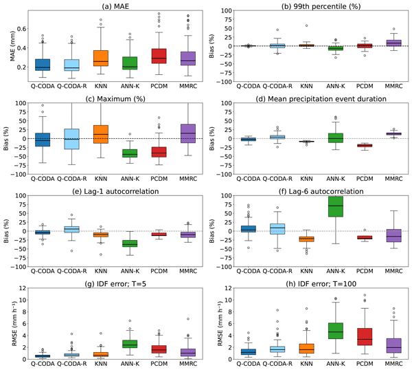
The results (Fig. 13) show that the regionalised semi-parametric version, Q-CODA-R, performs only slightly worse than the original station-calibrated Q-CODA, which has direct access to the target station's own historical record. Nevertheless, Q-CODA-R still outperforms several state-of-the-art disaggregation methods (KNN, ANN-K, PCDM, and MMRC) across a broad range of evaluation metrics, despite the fact that these competing methods were calibrated using observations from the target station itself. In particular, Q-CODA-R shows strong skill in reproducing sub-daily $P_{\mathrm{1}\mathrm{h}}^{\text{max}}$-related statistics, including MAE, upper percentiles, and absolute maxima, as well as key properties of the full hourly precipitation series, such as mean event duration and autocorrelation. It also yields lower errors in the reconstruction of IDF curves than several of the state-of-the-art methods. For more detailed information, see Figs. S8–S10 in the Supplement which show extended boxplots containing all metrics previously presented in Figs. 5, 6, and 8, respectively.

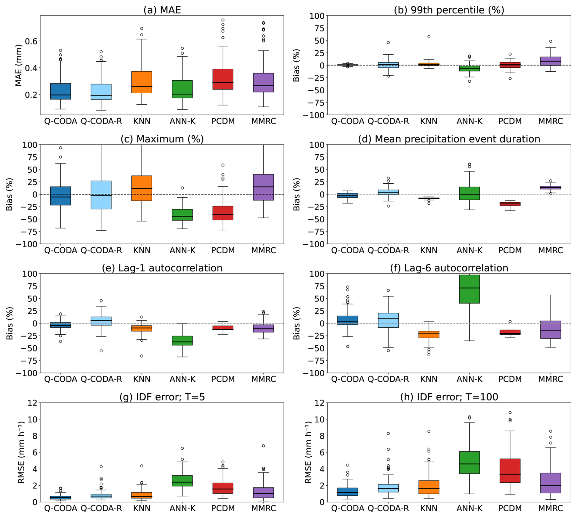
Figure 13 Comparative evaluation of disaggregation methods across 91 meteorological stations. Each panel shows boxplots summarizing the spatial distribution of key performance metrics: (a) Mean Absolute Error for $P_{\mathrm{1}\mathrm{h}}^{\text{max}}$ (MAE), (b) bias in the 99.th percentile for $P_{\mathrm{1}\mathrm{h}}^{\text{max}}$, (c) bias in maximum for $P_{\mathrm{1}\mathrm{h}}^{\text{max}}$, (d) bias in the mean precipitation event duration of the complete hourly series, (e) bias in the autocorrelation lag-1 of the complete hourly series, (f) bias in the autocorrelation lag-6 of the complete hourly series, (g) RMSE of the IDF curves for a 5-year return period, and (h) RMSE of the IDF curves for a 100-year return period. All methods except Q-CODA-R are evaluated using 5-fold cross-validation, whereas Q-CODA-R is evaluated in a leave-one-station-out (LOSO) framework, ensuring that no data from the target station are used in training Q-CODA-R.

8 Conclusions

This study introduced Q-CODA, a novel data-driven rainfall disaggregation framework that leverages the quasi-comonotonic relationship between daily precipitation totals and sub-daily maxima. Building on this empirically supported dependence structure, Q-CODA, through a comonotonic transformation, ensures that the simulated sub-daily maxima lie within plausible bounds conditional on the daily total, especially preserving the upper tail behaviour essential for extreme event modelling. Subsequently, Q-CODA initiates the disaggregation process by seeding an initial hourly pattern via a seasonal K-Nearest Neighbours (KNN) search, selecting and scaling realistic historical analogs. This pattern is then iteratively refined to satisfy both the daily total and the set of comonotonicity-based sub-daily maxima constraints across multiple durations (1 h, 2 h, 6 h, and 12 h). The adjustment procedure further enhances the temporal structure by increasing lag-1 autocorrelation through targeted reordering and smoothing, ensuring realism in the resulting rainfall sequences. This hybrid approach combines probabilistic rigor, empirical realism, and interpretability.

A comprehensive comparison against four existing methods – KNN, ANN-K, MMRC, and PCDM – demonstrates that Q-CODA consistently outperforms alternatives across a wide range of metrics. These include deterministic accuracy (e.g., MAE, NSE), distributional fidelity (bias in mean, variance, and high quantiles), and temporal structure (autocorrelation, event duration, dry hour frequency), evaluated across 91 stations in Spain. In particular, Q-CODA excels at reproducing extremes such as the 99th and 99.9th percentiles of hourly maxima and produces the lowest error in simulated IDF curves. The comparative performance of ANN-K highlights some benefits of deep learning in rainfall disaggregation, but also reveals important drawbacks, such as underestimation of variance and systematic misrepresentation of extremes, partially due to the limitations of neural networks in extrapolation beyond the training range. Traditional approaches such as MMRC and PCDM capture some statistical properties but show greater variability and biases across stations. Overall, Q-CODA emerges as a competitive, flexible, and physically grounded methodology for disaggregating daily rainfall into sub-daily time series. Its explicit use of dependence structures via comonotonic transformations, combined with an efficient constraint-based adjustment scheme, makes it well suited for hydrological modelling, flood risk assessment, and climate adaptation planning because it can be used for the extension of insufficient hourly precipitation data or the temporal disaggregation of climate change daily projections.

Additional analyses in independent climatic regions, including the Pacific Northwest and Florida (United States), confirm that Q-CODA maintains strong and stable performance under contrasting hydroclimatic conditions. These results support the transferability of the quasi-comonotonicity-based framework beyond Spain. In addition, sensitivity experiments, conducted using artificial precipitation series to ensure controlled dependence structures, further indicate that the performance of Q-CODA depends on the strength of the quasi-comonotonic relationship. When the Spearman correlation between daily totals and sub-daily maxima falls below approximately 0.975, the advantage of the comonotonic constraint begin to diminish, and KNN may become competitive, while also offering advantages in terms of lower computational cost and methodological simplicity.

To extend applicability beyond gauged locations, a semi-parametric regionalised version (Q-CODA-R) has been introduced, enabling spatial interpolation of model parameters and allowing application at ungauged sites. This version has been explicitly validated using a leave-one-station-out framework, demonstrating that the method can be meaningfully transferred beyond calibration locations and providing a first step towards spatial generalisation of sub-daily rainfall characteristics. However, despite this improvement, Q-CODA-R still operates at the level of independent pointwise predictions. The current formulation does not yet incorporate or evaluate full mesoscale hydrological consistency, particularly the joint spatial coherence of extreme events across multiple locations. In particular, it does not ensure the preservation of spatial dependence structures, the synchronisation of extremes between neighbouring sites, or the consistency of spatially continuous derived products such as gridded IDF surfaces. As such, while it represents a substantial advance over the original station-based formulation, it does not yet constitute a full mesoscale hydrological modelling framework. This limitation is important in the context of spatial applications, as the absence of an explicit spatial dependence model currently prevents direct use in fully distributed hydrological simulations. Nevertheless, the regionalised framework enables a practical pathway forward: applying Q-CODA-R to dense rain-gauge networks with only daily records, generating disaggregated sub-daily series at a much larger number of locations than currently possible with hourly observations. These reconstructed series could then be used to estimate local IDF curves, whose parameters could subsequently be spatially interpolated to derive gridded IDF products, following approaches such as Vicente-Serrano et al. (2025). In this sense, Q-CODA-R could represent an intermediate step towards mesoscale hydrological applications at sub-daily resolution in data-scarce regions. Future research may explore other promising directions. Coupling the methodology with regional climate model outputs could allow integration into broader downscaling frameworks. Moreover, increasing the temporal resolution from hourly to sub-hourly or minute-scale disaggregation is particularly relevant for high-resolution hydrological applications, including urban drainage, flash flood forecasting, and early warning systems, where rainfall dynamics at minute-level resolution are critical.