Which strategy to improve the performances of an LSTM-based model for extreme stream temperature values?

Deep-learning models have demonstrated strong performances in reproducing stream temperature dynamics, which is promising for the reconstruction of missing stream temperature records at ungauged locations. However, model accuracy over the range of high, summer stream temperature values has been usually overlooked, raising the question of the suitability of using deep-learning methods during this crucial season. In this study, we investigated strategies to improve the performances of a stream-temperature model based on LSTM (Long Short-Term Memory) cells over the extreme, highest 10 % observed values at 21 stations located in the Garonne river catchment. We quantified the gain in model performance thanks to regional multi-catchment training with static attributes, exploiting hydrologically relevant variables, and further penalizing the errors at extreme temperature values using custom loss functions. Our key results are: (1) Regional multi-catchment training is the best strategy to improve the performances of LSTM models not only over the extreme, top 10 % values but also over the whole range of observations. (2) The gain in performances was mainly brought by the use of static, catchment and reach attributes. (3) Customizing the loss function to emphasize the model errors on extreme temperature values did not lead to significant gains in test performances. This study further confirms the suitability of regionally trained LSTM models that exploit static attributes for the reproduction of extreme stream temperature values, offering significant advantages for water management at data-sparse regions.

1 Introduction

1.1 Challenges in stream temperature monitoring

Stream temperature is a key ecological variable that controls the biogeochemical equilibrium of river waters (Ducharne, 2008; Zhi et al., 2023), the spawning, growth, and health of aquatic species (Alfonso et al., 2021; Armstrong et al., 2021; Bowerman et al., 2018), and their spatial distribution along the river network (Bonacina et al., 2023; Buisson et al., 2008; Comte et al., 2013; Daufresne and Boët, 2007; Maire et al., 2019; Picard et al., 2022). Changes in stream temperature have strong impacts on drinking water production (Delpla et al., 2009), fisheries and related recreational activities (Jones et al., 2013), and can lead to disruption in electric energy production by impacting the cooling of power plants (van Vliet et al., 2012). Despite its ecological and socio-economic importance, existing monitoring networks of stream temperature are too recent (see Ouellet et al., 2020) and have a limited spatial coverage, leaving a significant number of reaches ungauged (Arora et al., 2016; Hannah and Garner, 2015). Furthermore, existing large-sample, nation-wide studies such as Beaufort et al. (2022), Hare et al. (2021), Orr et al. (2015) or Segura et al. (2015) illustrate the extent to which the characterization of the temporal variability of stream temperature can be limited due to low temporal resolution or high rates of missing values. For example, among the 1700 French stations collected by Beaufort et al. (2022), only 30 stations had year-round observations covering the whole 9-year period of study (2009–2017). This insufficient spatiotemporal monitoring not only limits the understanding of stream temperature variability at a variety of locations with contrasting landscape and climatic settings, but also the quantification and attribution of changes in stream temperature due to climate change or anthropogenic perturbations (Essaid and Caldwell, 2017; Kędra and Wiejaczka, 2018; Macedo et al., 2013; Moatar and Gailhard, 2006; Orr et al., 2015; Seyedhashemi et al., 2021; van Vliet et al., 2013).

1.2 Modelling approaches to overcome the monitoring gap: A brief overview

To overcome this monitoring gap, stream temperature models are typically applied to extend the existing records beyond their temporal coverage or reconstruct missing records at ungauged locations (via model regionalization). These models encode the interactions between stream temperature and other atmospheric and hydrological variables that are more widely available. A first modelling approach consists in explicitly specifying these interactions in the model structure by solving the energy budget at the reach scale. This energy budget accounts for heat advection along the watercourse and heat fluxes at the free surface and at the streambed interface (Caissie, 2006; Dugdale et al., 2017; Leach et al., 2023; Moore et al., 2005; Yearsley, 2009). Following this modelling approach, model parameters have a physical meaning and this facilitates the projection of changes in stream temperature in response to climate and landscape changes. Application examples include the characterization of the thermal regimes of large rivers using land surface models (Niemeyer et al., 2018; van Vliet et al., 2013; Wanders et al., 2019), the assessment of the impact of riparian shading at the reach scale (Dugdale et al., 2024), the quantification of heat exchanges at the stream-aquifer interface (Caissie et al., 2014; Kurylyk et al., 2015; Rivière et al., 2020), and the projection of future stream temperature under scenarios of climate drift (Michel et al., 2022). Unfortunately, fully solving the heat budget at the regional, catchment scale is computationally demanding and requires an expensive characterization of stream network morphology and other landscape parameters (such as land-use features). Therefore, process-based approaches resort to adopting several simplifying hypotheses, such as combining the physically based heat balance equation with a statistical approach (Gallice et al., 2015; Toffolon and Piccolroaz, 2015) or using the equilibrium temperature concept to parametrize the heat fluxes at the free surface (Edinger et al., 1968). For instance, variants of this concept have been compared at the Loire river catchment (∼10⁵ km²; Bustillo et al., 2014), with advanced model applications that explicitly account for hydrological processes, river network topology (e.g., Strahler order), and riparian vegetation (Beaufort et al., 2016; Seyedhashemi et al., 2023).

Alternative to the process-based approach, the implicit, fully data-driven approach aims at capturing the correlations between stream temperature and hydro-climatic variables using machine learning techniques (see the reviews in Gallice et al., 2015; Benyahya et al., 2007, and Souaissi et al., 2023). These techniques have less requirements in terms of data variety than process-based models and once trained, their computational cost in forward mode is more affordable. The most basic methods apply linear and logistic regression to estimate stream temperature from air temperature (Ducharne, 2008; Jackson et al., 2018; Mohseni et al., 1998; Stefan and Preud'homme, 1993). State-of-the-art applications account for hydrological and spatial controls on stream temperature in addition to atmospheric variables (Feigl et al., 2021; Isaak et al., 2014) and/or apply advanced machine-learning and deep-learning techniques to efficiently digest larger and more diverse data (Zhi et al., 2024). Among these techniques, models based on LSTM (Long Short-Term Memory; Hochreiter and Schmidhuber, 1997) have demonstrated excellent performances in predicting not only stream temperature but also several other dynamic, environmental variables (Arsenault et al., 2023; Kraft et al., 2025; Kratzert et al., 2018; Ma et al., 2021; Nearing et al., 2024; Song et al., 2024; Zhi et al., 2021). Sadler et al. (2022) showed the ability of LSTM models to predict both streamflow and stream temperature for 101 stations in the United States. Rahmani et al. (2021a) illustrated the excellent performances of LSTM models in reproducing stream temperature for 118 United States catchments, with a median RMSE (root-mean-square errors) at 0.69 °C. In particular, they showed an interesting application of a two-stage LSTM model, where an LSTM-based hydrological model provides streamflow simulations to an LSTM-based stream temperature model. Rahmani et al. (2021b) showed that regionally trained LSTM networks are very suitable for transferring information on stream temperature dynamics from monitored to unmonitored locations. Other studies demonstrated successful applications of LSTM networks for the more operational task of stream temperature forecasting (e.g., Padrón et al., 2025; Qiu et al., 2021; Zwart et al., 2023).

1.3 Research questions and scope of the paper

Our literature overview reveals that LSTM networks offer a very promising avenue for catchment-scale reconstruction of stream temperature for several reasons: (1) They provide state-of-the-art performances at several locations (Rahmani et al., 2021a, b); (2) Their performances improve when simultaneously trained at several locations thanks to their flexibility, which is suitable for regionalization (see Kratzert et al., 2024); (3) They can be physically constrained (De la Fuente et al., 2024; Hoedt et al., 2021) and their structure can be physically interpretable (Jiang et al., 2022; Lees et al., 2022). However, evaluation of LSTM performances for extreme values is limited to rainfall-runoff models (Frame et al., 2022; Nearing et al., 2024), and previous studies in the context of stream temperature modelling did not specifically address LSTM performances for extreme temperature values (Rahmani et al., 2021a, b). Extreme stream temperature values usually occur during the summer season, a highly critical period from a water-management standpoint, as it is concomitant with lower streamflow and higher air temperature values. Accurate predictions at this range are crucial to acceptably anticipate when the temperature values will exceed the legal/recommended threshold for drinking water production (25 °C according to the Council Directive 80/778/EEC; https://eur-lex.europa.eu/eli/dir/1980/778/oj/eng, last access: 22 May 2026) or the lethal/sub-lethal thresholds for freshwater species (see Jackson et al., 2018).

Our objective is thus to address this research gap by exploring the performances of an LSTM-based model for daily stream temperature at 21 stations in the Garonne river catchment (∼10⁴ km²). This catchment faces several water management challenges especially during the summer season due to high anthropogenic pressure (agriculture, hydro-electricity, and urbanization). Paradoxically, very few studies have addressed stream temperature modelling at this catchment (Beaufort et al., 2022; Larnier et al., 2010). In our implementation, we focused on strategies to improve LSTM performances for extreme daily stream temperature values (top 10 % of the daily observations), while at the same time maintaining satisfactory performances for the remaining range of daily records. Specifically, we compared 18 loss functions, local vs. regional/multi-catchment training, and several combinations of static and dynamic input variables. We aimed at answering the following research questions:

• To improve the reproduction of extreme, high stream temperature values, what can be gained from increasing the weight of extreme stream temperature values in the loss function used for training?

• How does this strategy compare to a careful selection of the input variables? In particular, what is the contribution of hydrologically relevant variables (namely streamflow)?

• What is the added value of combining regional training with static, catchment and reach attributes in improving the performances of LSTM-based models for extreme, high stream temperature values?

The remaining of this manuscript is organized as follows. Section 2 will present the catchment set, the collected stream temperature dataset, and the dynamic and static variables used to implement the LSTM models. Section 3 will detail the methodological setup and the tested strategies to improve LSTM performances for extreme, high stream temperature values. Sections 4 and 5 will show and discuss the results, and Sect. 6 will summarize the main findings and propose some future research directions.

2 Catchment set

We used pre-processed daily stream temperature (T_w) time series provided by the Haute-Garonne Departmental Council (CD31) at 37 stations located within the Garonne catchment upstream of Toulouse, France (Fig. 1). Among these stations, only 21 stations have more than 2434 daily observations of T_w, which is required to ensure a minimum of one year (365 d) of datapoints for model testing (see Sect. 3.2; 15 % of the available T_w datapoints were dedicated to model testing, therefore we required a minimum of $\mathrm{365}/\mathrm{0.15}=\mathrm{2433.33}$ or 2434 datapoints in total). We call these 21 stations “test stations” since they are the only stations with enough datapoints to allow for robust model testing (see Sect. 3.2.2 for more details). Raw T_w time series span years within the period 1991–2021 and were provided by different sources:

• Data for 12 stations were extracted from the Naiades database (https://naiades.eaufrance.fr/acces-donnees#/temperature, last access: 18 April 2026), which is managed at the national scale by the French Office for Biodiversity (Office Français de la Biodiversité). Among these stations, $\mathrm{10}/\mathrm{12}$ are test stations;

• Five stations are part of the alert network (Réseau des Stations d'Alerte, RSA), which monitors the water quality at specific locations close to withdrawal points for drinking water production. Among these stations, $\mathrm{3}/\mathrm{5}$ are test stations;

• Data for 20 stations were provided by two departmental federations for fishing: FPeche31 (Fédération de Pêche de la Haute-Garonne), FPeche65 (Fédération de Pêche des Hautes-Pyrénées), and one additional fishing association: MIGADO (Migrateurs Garonne Dordogne Charente Seudre). Among these stations, $\mathrm{8}/\mathrm{20}$ stations are test stations.

This diversity of data providers poses a challenge from a standpoint of data quality and data uncertainty. For example, some of the 21 test stations are located very close to each other but their T_w time series come from different sources. This is the case of four pairs of stations (see Fig. 1 for their location): (1) two stations that are located on the Garonne river at Bazacle (Toulouse) and their T_w data were provided by RSA and MIGADO; (2) two stations that are located on the Garonne river at Valentine (Naiades and MIGADO); (3) two stations that are located on the Pique river at Cier-de-Luchon (Naiades and MIGADO); and (4) two stations that are located on the Garonne river at Labarthe-Inard/Montespan (Naiades and RSA). Since these stations are still away from each other and their time series showed some differences (due to sensor location and exposure), we decided to keep them all since there was no additional information that could have helped decide which stations to discard.

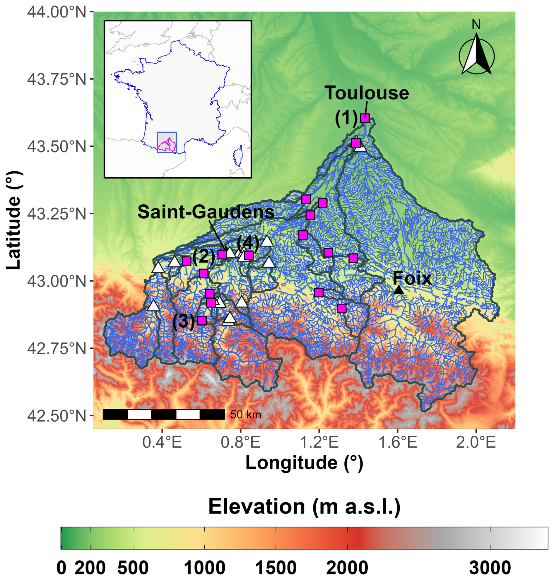
Figure 1 Location of the Garonne catchment and the 37 stream temperature stations used in this study. Test stations (i.e., stations having at least 2434 daily observations of stream temperature) are shown with magenta rectangles, whereas stations used only for the training of regional models are shown with white triangles. Elevation values were extracted from the SRTM GL3 product (90 m resolution). River network was extracted from BD CarTHAgE^®. Numbers (1), (2), (3), and (4) indicate the location of the river reaches with a pair of stations close to each other but with stream temperature data collected from two different sources.

For each T_w station, we extracted hourly air temperature values from the SAFRAN dataset (SAFRAN stands for Système d'Analyse Fournissant des Renseignements Atmosphériques à la Neige; Quintana-Seguí et al., 2008; Vidal et al., 2010). This dataset was provided by Météo-France at a resolution of 8 km. From the hourly time series, we computed daily mean air temperature (T_a) and maximum and minimum air temperature for each day (T_amx and T_amn).

In addition to station-scale atmospheric forcing, we also collected catchment-scale hydrologically relevant variables to quantify their contribution in improving T_w predictions, especially for the case of summer, high T_w values. The first set of hydrologically relevant variables is composed of catchment-scale precipitation (P) and potential evapotranspiration (PE) time series at the daily time step. First, we delimited the topographic catchment drained by each T_w station using the PyFlwDir Python library (version 0.5.8; Eilander et al., 2021) with the 30 m SRTM dataset for elevation values (SRTM stands for Shuttle Radar Topography Mission; Farr et al., 2007). We did not choose the national product BD ALTI^® because it does not cover the very upstream part of the Garonne catchment located in Spain. Second, we used the catchment polygon to extract spatial averages of precipitation values from the hourly, 1 km COMEPHORE dataset (COMEPHORE stands for COmbinaison en vue de la Meilleure Estimation de la Précipitation HOraiRE; Tabary et al., 2012), then we summed the hourly values for each day to obtain the daily time series. Third, we used the catchment polygon to extract spatial averages of air temperature values from the SAFRAN dataset, then we applied a temperature-based formula to compute daily potential evapotranspiration from the daily averages of air temperature (Oudin et al., 2005). The second set of hydrologically relevant variables consists of streamflow (Q_sim). Since existing streamflow gauging stations did not coincide with the set of T_w stations, we reconstructed streamflow records at each T_w station by feeding the time series of precipitation and potential evapotranspiration to the daily hydrological model GR6J (Pushpalatha et al., 2011), with a parameter transfer approach based on spatial proximity (see Appendix A for details).

Finally, we computed a set of static variables that we used to construct regionally trained LSTM models for T_w (Table 1). These static variables were chosen to reflect catchment properties in terms of climate (aridity index, i.e., ratio of average potential evapotranspiration to average precipitation for the catchment), morphology (station elevation, median catchment elevation, catchment area), land use (percent of urban areas, forest cover, and agricultural areas), and soil (percent of sand, clay, and silt). This relatively small dataset covers a rather rich gradient of climatic and landscape characteristics, with cold thermal regimes and steep orographic gradients upstream vs. warm thermal regimes and mild slopes downstream (see Table 1 and Fig. 1). Note that some of these stations are located close to hydroelectric power plants or downstream of a retention pond, offering a rich mixture of natural and anthropogenically impacted thermal regimes.

Table 1 Summary of dynamic and static variables and their distributions across the catchment set. Min, median, and max values were computed from the set of 37 stations, except for the long-term averages of daily stream temperature.

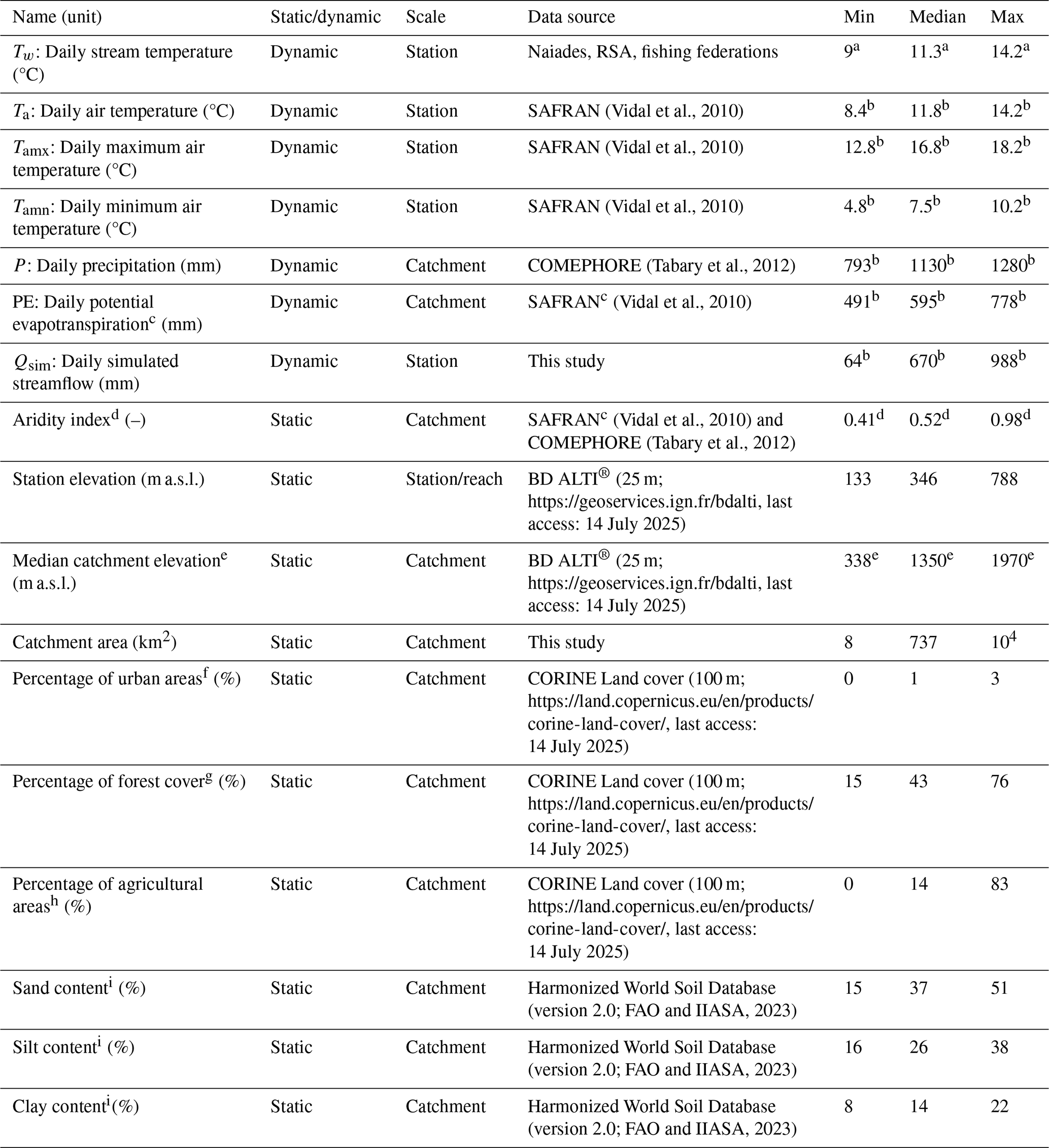
^a We first computed, for each station, the long-term average of stream temperature values using the whole time series, which gave 37 values. We then excluded the stations with short time series by computing min, median, and max statistics using the 21 test stations only. ^b These values represent long-term averages (1997–2022) in °C for temperature and in mm/year for precipitation, potential evapotranspiration, and simulated streamflow. ^c We estimated potential evapotranspiration using a temperature-based formula (Oudin et al., 2005). Air temperature was extracted from SAFRAN (resolution of 8 km). ^d Aridity index was computed as the ratio of long-term catchment-average potential evapotranspiration to long-term catchment-average precipitation over the period 1997–2022. ^e We obtained similar statistics using the more complete SRTM GL1 dataset (30 m resolution): 341, 1360, and 1970 m for min, median, and max values. ^f We took the average over the years 1990 to 2018 of the proportion of the catchment occupied by the following CORINE land-cover classes: classes belonging to 1.1 (Urban fabric), 1.2.1 (Industrial or commercial units and public facilities), and 1.2.2 (Road and rail networks and associated land). ^g We took the average over the years 1990 to 2018 of the proportion of the catchment occupied by the CORINE land-cover classes under 3.1 (Forest). ^h We took the average over the years 1990 to 2018 of the proportion of the catchment occupied by the CORINE land-cover classes under 2 (Agricultural areas). ⁱ We took the catchment-scale average over the seven layers (0–20, 20–40, 40–60, 60–80, 80–100, 100–150, and 150–200 cm) using the hwsdr R package (Hufkens, 2021).

3 Tested strategies to improve the performances of LSTM models over extreme stream temperature values

3.1 Model structure

Our choice of LSTM networks to implement a model for T_w is motivated by four main reasons: (1) They demonstrated state-of-the-art performances across several catchments (Rahmani et al., 2021a); (2) They allow for incorporating static in addition to dynamic variables, which is suitable for regionalization (Hashemi et al., 2022; Kratzert et al., 2019; Rahmani et al., 2021b; Yu et al., 2024); (3) They are strong spatial extrapolators by performing better in a regionalization mode (Kratzert et al., 2024), which opens the way for reconstructing the missing records at ungauged locations; and (4) They are more flexible than process-based approaches in handling measurement uncertainties and accounting for anthropogenic influences by inferring the influenced T_w behaviour directly from the observations.

We conducted a preliminary study in which we tested several hyperparameters to see their impact on the LSTM performances (not shown here). We concluded the following:

• The LSTM performances were not significantly sensitive to the number of LSTM layers or the number of LSTM cells per layer. For this reason, we chose to test an LSTM model with only one layer composed of 128 LSTM cells, with a dropout rate at 0.4 to limit the risk of overfitting (Srivastava et al., 2014), and connected to the output layer (1 neuron) via a dense layer of 128 neurons activated using a linear function.

• The LSTM performances were sensitive to the lookback, which was expected due to the strong differences in T_w dynamics across our catchment set. For this reason, we chose to test three lookbacks (30, 90, 365) to accommodate for T_w dynamics at the monthly, seasonal, and annual scales. Our strategy to choose the best lookback value among the three tested values is based on splitting our data sample into three subsets for training, validation, and test of the LSTM models (see Sect. 3.2.2 for more details), and then keeping only the lookback value that minimized model errors on the validation set. More details are provided in Sect. 3.3.

• The LSTM performances were not sensitive to the batch size, which we fixed at 64. In addition, we chose Adam (Kingma and Ba, 2017) as an optimizer with a fixed learning rate at 10⁻⁴. The maximum number of epochs was fixed at 10 000. However, we implemented an early stopper that halted the training of the LSTM after 100 epochs with no decrease in MSE (mean squared errors) on the validation set by at least 0.001 °C².

A detailed description of the LSTM equations can be found in Hashemi et al. (2022) or Kratzert et al. (2018). Our LSTM models were implemented and trained using classes and functions from the PyTorch library (Paszke et al., 2019) in a Python development environment (version 3.8).

3.2 Strategies to improve the LSTM performances for extreme stream temperature values

In this section, we summarize the strategies that we tested to look for the best approach to improve the LSTM performances at extreme, high T_w values. We define these values as the daily (average) T_w values exceeded less than 10 % of the time. Our tested strategies include an adaptation of the loss function to increase the weight of extreme values in the training phase (Sect. 3.2.1), regional multi-catchment training (Sect. 3.2.2), and the inclusion of hydrologically relevant variables and static attributes (Sect. 3.2.3).

3.2.1 Option 1: Adaptation of the loss function

To improve the performances of the LSTM model for a specific range of the target variable, a potential strategy consists in emphasizing the model errors on the range of interest by increasing their weight in the loss function. This is a common strategy for example in the calibration of hydrological models (Garcia et al., 2017; Pushpalatha et al., 2012; Saadi and Furusho-Percot, 2024; Thirel et al., 2024). We thus tested 18 loss functions that share the following general expression:

$$\begin{array}{}\text{(1)}& L\left(T_{w,\mathrm{sim}},T_{w,\mathrm{obs}}\right)={\displaystyle \frac{\sum _t{\left|g{\left(T_{w,\mathrm{obs},t}\right)}^{\mathit{\mu }}-g{\left(T_{w,\mathrm{sim},t}\right)}^{\mathit{\mu }}\right|}^{\mathit{\lambda }}}{\sum _t{\left|g{\left(T_{w,\mathrm{obs},t}\right)}^{\mathit{\mu }}-\stackrel{\mathrm{‾}}{g{\left(T_{w,\mathrm{obs}}\right)}^{\mathit{\mu }}}\right|}^{\mathit{\lambda }}}}\end{array}$$

where $T_{w,\mathrm{sim},t}$, $T_{w,\mathrm{obs},t}$ represent the simulated and the observed T_w values at the time step t, $g\left(T_{w,\mathrm{sim},t}\right)$, $g\left(T_{w,\mathrm{obs},t}\right)$ their transformed values using the function g, and μ, λ are hyperparameters. For an intuitive interpretation of this function, the denominator in the loss function of Eq. (1) standardizes the values of the loss function by comparing the performances of the LSTM model to a “dummy” model that gives the average value of the transformed observations $\stackrel{\mathrm{‾}}{g{\left(T_{w,\mathrm{obs}}\right)}^{\mathit{\mu }}}$ as a prediction for all the time steps. This denominator plays also the role of a normalizing constant without which the learning rate should be adapted to account for the larger error magnitudes in the numerator induced by higher values of λ and especially μ. This last hyperparameter μ results in magnitudes of g(T_w) that are higher at extreme values than at mild values, inducing larger errors at (and thus more emphasis on) extremely high values. In our implementation, the loss function of Eq. (1) is evaluated per batch and accordingly, the denominator changes depending on the observed T_w values within the batch. We tested all the possible combinations from the following configurations:

• Three values for μ: 1, 3, and 5;

• Three values for λ: λ=2, which corresponds to using MSE as a metric; λ=1 which corresponds to MAE (mean absolute errors); and λ=4, which we refer to by M4E (mean errors to the power 4);

• Two functions for g: g(T)=T (non-standardized target) and $g\left(T\right)=\frac{T-m}{\mathit{\sigma }}$ (standardized target), where m and σ correspond to the mean and the standard deviation of the observed T_w values computed on the training set.

Among our tested choices, emphasizing the weight of high T_w values in the loss function is achieved by increasing the values of λ, μ, and avoiding standardization (g(T)=T). Note that the commonly chosen loss function (hereafter, the “reference” loss function) corresponds to the combination of μ=1, λ=2 (MSE) and $g\left(T\right)=\frac{T-m}{\mathit{\sigma }}$.

3.2.2 Option 2: Regional training

Due to its flexibility, an LSTM-based model has the ability to learn from a large space of thermal behaviours when trained in a regionalization mode (i.e., simultaneously at multiple catchments), which may result in better performances for the range of extreme values (Kratzert et al., 2024). Moreover, it offers the possibility of using static, catchment and reach attributes in addition to dynamic variables (see Sect. 3.2.3). In this regard, for each test station (21 in total), we compared two different sets of models:

1. The set of local models trained using the first 70 % of the available T_w records and their corresponding input, dynamic variables only at the station of interest. In this case, half of the remaining T_w observations (i.e., 15 % of the available records) were used for validation and the remaining records (i.e., 15 % of the available records) were kept for test. Note that for these stations, 15 % of the available records span at least one-year worth of daily observations.

2. The set of regional models trained using data from all the 37 stations. In this case, we constructed the training set by concatenating 70 % of the available T_w and their corresponding input variables from each station. The validation set was constructed using 15 % of observations at the test stations ($\mathrm{21}/\mathrm{37}$) and the whole remaining 30 % of observations at the non-test stations ($\mathrm{16}/\mathrm{37}$). Finally, the remaining 15 % of observations at the 21 test stations were used to test the regional models, thus enabling a comparison of locally and regionally trained models on the same datapoints. Although 30 % of the observations at the non-test stations were used in the validation set against 15 % from the test stations, datapoints from the test stations still constituted up to 78 % of the validation set due to the lower availability of T_w records at non-test stations.

Note that this methodological setup does not fully examine the LSTM capabilities in spatial extrapolation as done by Rahmani et al. (2021b) or Yu et al. (2024) for a more challenging spatial extrapolation of hydrological regimes between regions with contrasting climatic and landscape settings. Implementing these more rigorous setups would have required either holding a subset as pseudo-ungauged for testing, or adopting a leave-one-out approach (Jackson et al., 2018), and these two options are limited by the size of our catchment set and the large number of tests that we already performed. However, our methodological setup will still indicate the extent to which the multi-catchment training helps the regionally trained LSTM models in learning from all the catchment behaviours at once and performing better than the locally trained ones, which is necessary (although not sufficient) for satisfactory spatial extrapolation performances.

3.2.3 Option 3: Choice of the input variables

The most basic T_w models make use of the strong correlation between T_w and air temperature (T_a). Here, we quantify the added value of using catchment-scale hydrological variables especially for the simulation of high T_w values. In addition, we examine the added value of static, catchment and reach attributes using the regionally trained LSTM models. In summary:

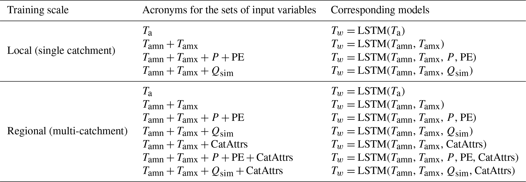
1. We tested four sets of input variables for the local models (Table 2). Comparing models that use T_a against those using T_amn+T_amx as inputs will show whether there is any added value in using daily extreme air temperature values instead of the daily averages. The added value of hydrological variables will be evaluated by comparing models that use $T_{\mathrm{amn}}+T_{\mathrm{amx}}+P+\text{PE}$ and $T_{\mathrm{amn}}+T_{\mathrm{amx}}+Q_{\mathrm{sim}}$ against those using T_amn+T_amx. Finally, comparing $T_{\mathrm{amn}}+T_{\mathrm{amx}}+P+\text{PE}$ and $T_{\mathrm{amn}}+T_{\mathrm{amx}}+Q_{\mathrm{sim}}$ will show whether the LSTM models are able to maintain similar (or obtain better) performances by exploiting the catchment-scale forcing (P and PE, with PE being a good proxy for catchment-average air temperature according to the temperature-based formula in Oudin et al., 2005) instead of the more relevant station-scale streamflow (Q_sim).

2. We tested seven sets of input variables for the regional models (Table 2). Four of the seven sets are the same sets of input variables that we used for the local models in order to measure the added value of regional, multi-catchment training. In addition, we tested three more sets that include 10 static, catchment and reach attributes (CatAttrs) in addition to dynamic inputs (see Table 2). Comparing these sets with the ones using only the dynamic inputs will help us quantify the gain in accuracy brought by the static attributes.

Note that to feed the LSTM model with the static attributes, we opted for a simple integration strategy (see, e.g., Hashemi et al., 2022) in which we repeated the value of each static attribute at each time step to match the length of the dynamic attributes, then we concatenated the columns of the static attributes to those of the dynamic attributes (for each catchment). This strategy compared well against a separate processing of static attributes from dynamic ones using an entity-aware (EA) variant of LSTM networks (Kratzert et al., 2019), and better strategies to encode the static attributes as well as the dynamic variables as inputs to LSTM models have been recently intercompared by Kraft et al. (2025). For both sets of local and regional models, all the input data were standardized using moments (mean, standard deviation) computed on the training set. Finally, we avoided using time-based features (month or day of the year; Feigl et al., 2021) so that the performances of the tested LSTM models remain comparable to process-based models that do not benefit from feature engineering. In addition, knowing the strong seasonality of T_w and of some of the input variables (T_a, T_amn, T_amx, and PE), the use of time-based features would be redundant information-wise and would likely lead to gains in predictive performances high enough to overshadow the contribution of the more physically relevant variables used in our setup.

Table 2 Summary of tested local and regional models. “CatAttrs” refers to static, catchment and reach attributes (see Table 1). Reach attributes include only station elevation. Catchment attributes consist of aridity index, mean catchment elevation, catchment area, land cover properties (percentage of urban, forest, and agricultural areas), and soil properties (sand, silt, and clay content).

3.3 Evaluation framework

We repeated each training configuration (local vs. regional training, input variables, loss functions) three times corresponding to each of the three pre-chosen lookback values (30, 90, and 365), meaning that we trained a total of $\mathrm{3}\times \mathrm{4}\times \mathrm{18}\times \mathrm{21}=\mathrm{4536}$ local models and $\mathrm{3}\times \mathrm{7}\times \mathrm{18}=\mathrm{378}$ regional models. For each configuration, we kept only the lookback value that provided the lowest MSE on the validation set (in other words, we optimized the lookback value on the validation set). Thus, we evaluated a total of $\mathrm{4}\times \mathrm{18}=\mathrm{72}$ local models and $\mathrm{7}\times \mathrm{18}=\mathrm{126}$ regional models on each of the 21 test stations, which do not necessarily share the same lookback value. To quantify model performances, we computed the mean absolute error MAE (in °C) between the predictions of each model and the observed values during the test period. We chose MAE as an evaluation metric simply because it allows for easier interpretation of model performances. We computed the MAE score first on the whole test period, then on a restricted period during which observed T_w exceeded the 90th percentile, which corresponds to the 10 % highest T_w values observed during the test period. Targeting higher ranges of extreme T_w values (for example, top 5 % or 1 %) is limited in our case by the relatively short test samples available at our 21 test stations, which have sizes that vary from 390 to 1074 d. To control whether choosing MAE as an evaluation metric favours MAE-based loss functions, we also evaluated the model performances using RMSE as an evaluation metric instead of MAE (see Appendix C for the corresponding results).

To evaluate the statistical significance of the differences between two options, say A and B, we applied a one-sided binomial test according to which the null hypothesis is “the proportion of cases where option B outperforms option A is lower than or equal to 50 %” (Fidal and Kjeldsen, 2020; Saadi et al., 2021). Here, “outperforms” means scoring lower MAE (or RMSE) values on the test period. We rejected the null hypothesis when option B scored better performances than option A for a sufficiently high number of cases that is defined by the threshold of significance. For example, if the total number of cases is 21 (e.g., 21 stations), we rejected the null hypothesis at the significance level of 5 % (respectively of 0.1 %) when option B outperformed option A in more than $\mathrm{15}/\mathrm{21}$ cases (respectively $\mathrm{18}/\mathrm{21}$ cases), in which case we concluded that the use of option B brought statistically significant improvements compared to option A.

4 Results

In this section, we first show the added value of changing the loss function (Sect. 4.1). Then, we show the performances of the local models (Sect. 4.2). Finally, we show the performances of the regionally trained models and the added value of using static, catchment and reach attributes (Sect. 4.3). For information, statistics for the wall-clock time needed to train the LSTM models are given in Table B1 (see Appendix B).

4.1 Effect of the loss function

Unexpectedly, increasing the weight of high T_w values in the loss function deteriorated the performances not only for the reproduction of extreme T_w values (top 10 %), but also for the reproduction of the whole range of T_w observations (Figs. 2 and C1 in Appendix C). In detail:

• The best performances over the whole period were systematically obtained using MAE (with or without standardization) as a loss function in the training: median test MAE reached 0.72 °C for the local models (all configurations of input variables combined, Fig. 2a) and 0.77 °C for the regionally trained models (Fig. 2b). In comparison to the reference loss function (MSE on standardized target), improvements with MAE as a loss function were statistically significant only in the case of locally trained models, for which MAE applied to standardized and non-standardized target resulted in better performances than the reference loss function for $\mathrm{58}/\mathrm{84}$ and $\mathrm{54}/\mathrm{84}$ cases, respectively (recall that the number of cases is the number of the test stations times the number of sets of input variables, see Table 2). For the regional models, MSE without standardization is the only loss function that resulted in statistically better performances, with better scores than the reference loss function for $\mathrm{85}/\mathrm{147}$ cases, which is higher in this case than the 5 %-significance threshold ($\mathrm{84}/\mathrm{147}$).

• Compared to the whole-range performances, model performances were systematically lower on the top 10 % range. For this range, the best median performances were obtained using MAE/M4E with standardization for the local models (1.07 °C, Fig. 2a) or using MSE without standardization for the regional models (0.98 °C, Fig. 2b). However, these improvements were not statistically significant at the 5 %-level in comparison with the reference loss function (MSE with standardization): For the local models, MAE with standardization resulted in better performances compared to the reference loss function for only $\mathrm{48}/\mathrm{84}$ cases, which is below the 5 %-significance threshold ($\mathrm{51}/\mathrm{84}$); For the regional models, MSE without standardization gave better scores than the reference loss function for only $\mathrm{70}/\mathrm{147}$ cases.

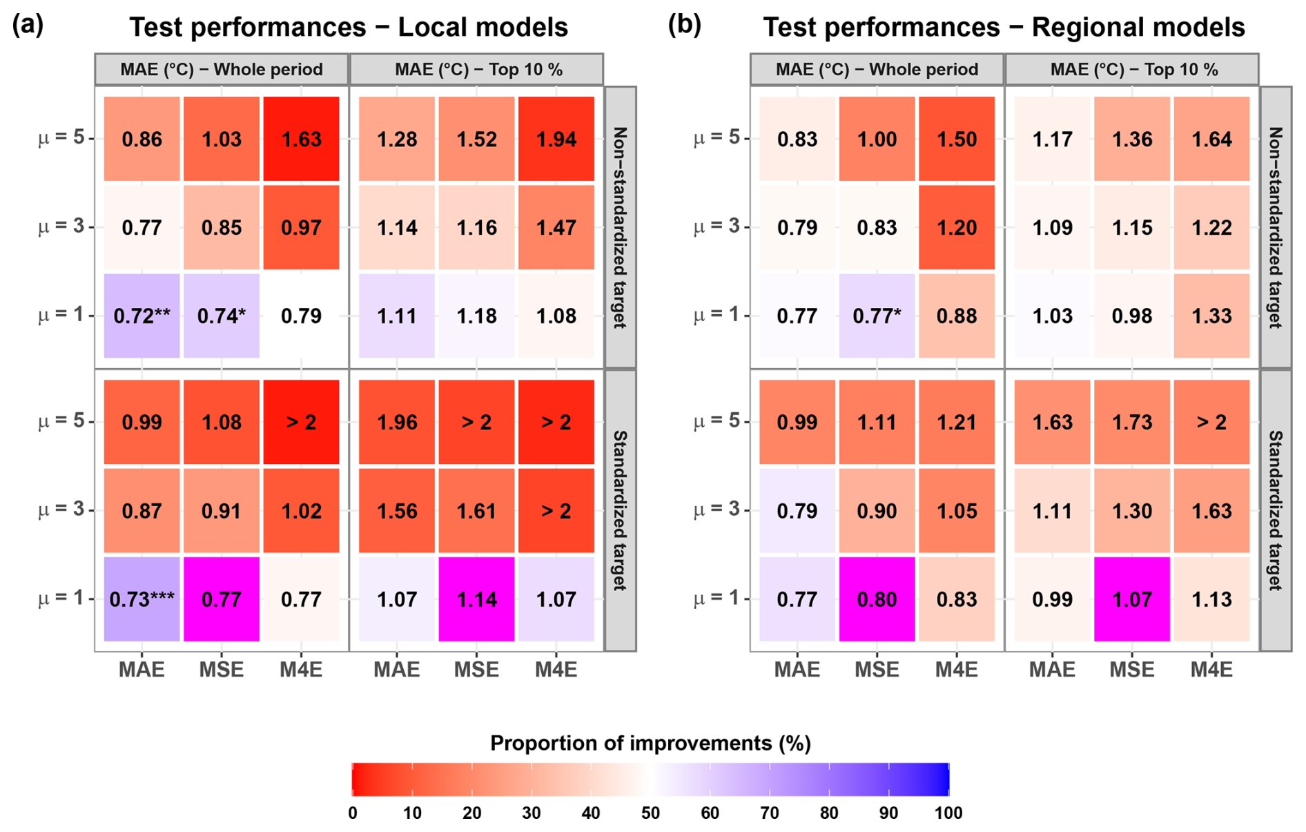
Figure 2 Median test performances (MAE, in °C) of the local models (a) and the regional models (b) according to the loss function used for training. These median values were computed from a set of $\mathrm{21}\times \mathrm{4}=\mathrm{84}$ points for the local models and $\mathrm{21}\times \mathrm{7}=\mathrm{147}$ points for the regional models. Note that the models we kept for test do not necessarily share the same lookback. Colours indicate the proportion of cases for which the use of the loss function yielded better results than the reference loss function (MSE with standardization, shown in magenta). Asterisks indicate that the custom loss function is significantly better than the reference loss function according to the one-sided binomial test: * for a significance threshold of 5 %, ** for a threshold of 1 %, and *** for a threshold of 0.1 %.

4.2 Performances of the local models

Using catchment-scale atmospheric forcing (precipitation and potential evapotranspiration) in addition to station-scale atmospheric forcing led to the best results with the local models (Fig. 3). More specifically:

• Over the whole period, the best median performances were obtained with $T_{\mathrm{amn}}+T_{\mathrm{amx}}+P+\text{PE}$ as input variables (median MAE at 0.65 °C, MAE without standardization as the best training loss function for this range; see Fig. 2a). Over the top 10 % range, the best median performances were also obtained with $T_{\mathrm{amn}}+T_{\mathrm{amx}}+P+\text{PE}$ as input variables (median MAE at 0.95 °C, MAE with standardization as a loss function).

• The use of daily min/max air temperature (T_amn+T_amx) instead of daily average air temperature (T_a) did not always result in significantly better performances according to the one-sided binomial test.

• The use of the hydrological variables (P+PE or Q_sim) always led to better results than using only station-scale air temperature (T_a or T_amn+T_amx), especially over the top 10 % range. However, these improvements were not always statistically significant.

• The use of simulated streamflow (Q_sim) instead of catchment-scale atmospheric forcing (P+PE) led to comparable performances over both the whole range and the top 10 % range, suggesting the similarity of catchment-scale forcing and station-scale simulated streamflow in terms of the information content extracted by the LSTM models.

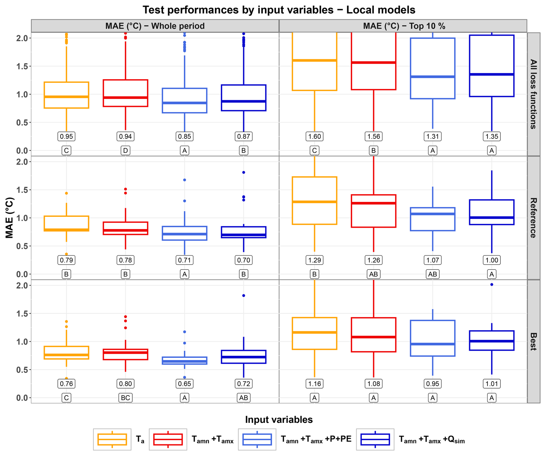
Figure 3 Distributions of the test performances (MAE, in °C) of the local models over the whole test period (left column) and the test subperiod corresponding to the highest 10 % observed values (right column). The top row shows the distributions over all the loss functions ($\mathrm{18}\times \mathrm{21}=\mathrm{378}$ points per distribution). The middle row shows the performances for the reference loss function, MSE with standardization, for both the whole period and the top 10 % range (21 points per distribution). The bottom row shows the performances for the best loss function over all sets of input variables (MAE without standardization for the whole period and MAE with standardization for the top 10 % range, 21 points per distribution). Numerical values under the boxes represent the median value for each distribution. Letters under the numerical values rank the distributions, and are defined such as distributions that share at least one letter are not significantly different according to the one-sided binomial test. Note that the models we kept for test do not necessarily share the same lookback.

4.3 Performances of the regional models

The use of static, catchment and reach attributes led to the best performances over both the whole test period and the top 10 % range (Fig. 4). More specifically:

• Over the whole test period, the best performances were obtained by exploiting catchment-scale atmospheric forcing (P+PE) in addition to static attributes (median MAE at 0.56–0.57 °C). Over the top 10 % range, the best performances (median MAE at 0.73–0.74 °C) were obtained by the models that exploited either the catchment-scale atmospheric forcing (P+PE) or the simulated streamflow (Q_sim) depending on the loss function used for training.

• In general, simply training the LSTM at the regional scale led to deteriorated median performances, as can be seen by comparing regionally trained models without static attributes with their counterparts in Fig. 3 (all loss functions and reference loss function; note that the best loss function changes between the whole-period and the top-10 % evaluation).

• The improvements brought by using the static attributes were almost always statistically significant according to the one-sided binomial test. Exceptions are limited to some performance distributions over the top 10 % range (namely, models taking as inputs T_amn+T_amx with vs. without static attributes with the reference loss function, and models taking as inputs $T_{\mathrm{amn}}+T_{\mathrm{amx}}+P+\text{PE}$ with vs. without static attributes with the best loss function; see Fig. 4).

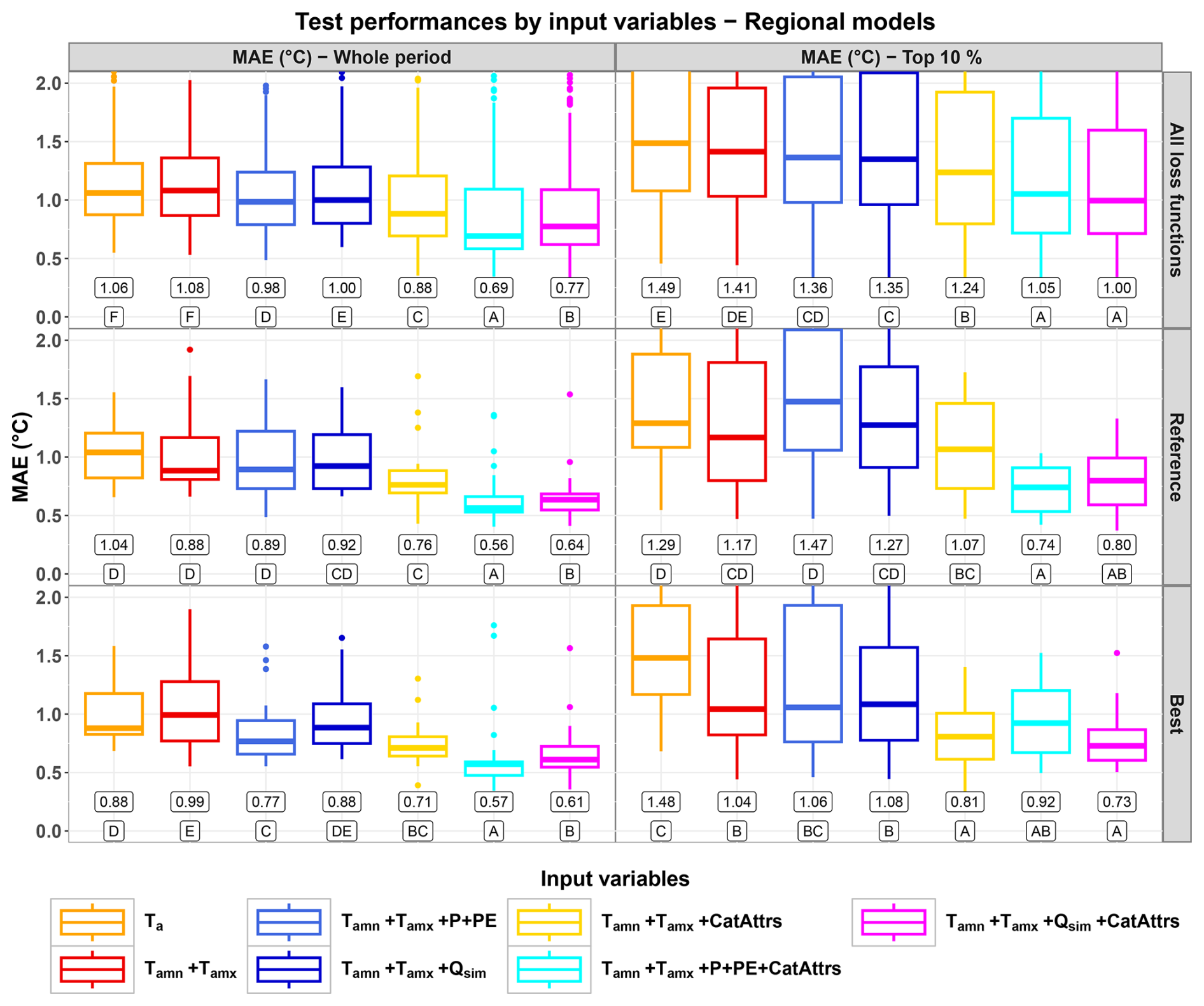
Figure 4 Distributions of the test performances (MAE, in °C) of the regionally trained models over the whole test period (left column) and the test subperiod corresponding to the highest 10 % observed values (right column). The top row shows the distributions over all the loss functions ($\mathrm{18}\times \mathrm{21}=\mathrm{378}$ points per distribution). The middle row shows the performances for the reference loss function, MSE with standardization, for both the whole period and the top 10 % range (21 points per distribution). The bottom row shows the performances with the best loss function over all sets of input variables (MAE with standardization for the whole period and MSE without standardization for the top 10 % range, 21 points per distribution). Numerical values under the boxes represent the median value for each distribution. Letters under the numerical values rank the distributions, and are defined such as distributions that share at least one letter are not significantly different according to the one-sided binomial test. Note that the models we kept for test do not necessarily share the same lookback.

To illustrate the improvements brought by the static attributes for regionally trained models, an example of model simulations is shown in Fig. 5 for the Garonne at Valentine (T_w data provided by MIGADO). This station is located at an altitude of 360 m, and drains a catchment area of 2260 km² with a median altitude of the catchment at 1390 m. The T_w observations for this station range between 2 and 21 °C over the whole period of records (2007–2021), with a 90 % percentile at 17.8 °C over the test period (2019–2021). Regionally trained models with only dynamic variables as inputs produced satisfactory results over the whole period (MAE at 0.74–0.86 °C, Fig. 5a) with a slight improvement thanks to the catchment-scale climatic inputs, but a significant degradation of model performances can be noticed over the top 10 % (MAE at 1.18–1.34 °C, Fig. 5c). The use of static attributes improved the performances not only over the whole period (MAE down to 0.48 °C, Fig. 5b), but also over the highest 10 % values (MAE down to 0.48 °C, Fig. 5d).

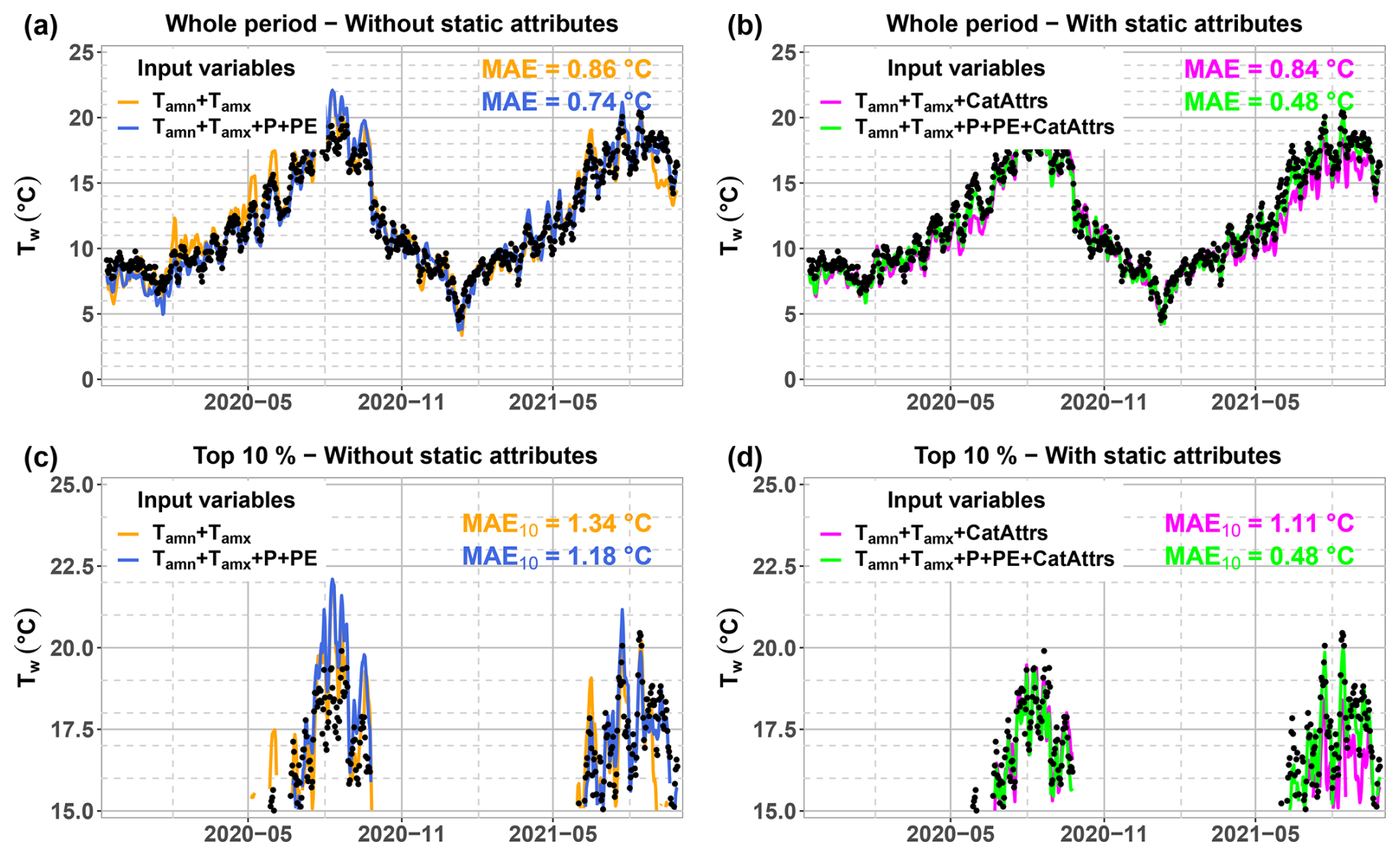
Figure 5 Example of model simulations using LSTM against observations at the station of the Garonne at Valentine (MIGADO). All models shown here were regionally trained. The two top figures (a, b) show the model simulations and performances (MAE, in °C) over the whole test period, and the two bottom figures (c, d) zoom in on the highest 10 % of the observations during the test period. Note that for bottom figures, the minimum value was fixed at 15 °C whereas the 90 % percentile is at 17.8 °C, with performance values computed using only the time steps when the observed values were equal or above the 90 % percentile. Input variables include station-scale daily minimum and maximum air temperatures (T_amn+T_amx) in addition to catchment-scale precipitation and potential evapotranspiration (P+PE). Models that use static attributes among input variables are shown on the right (b, d), while models that use only dynamic variables are shown on the left (a, c).

5 Discussion

To our knowledge, very few studies focused on model performances over periods with extremely high T_w values (a very close example can be found in Jackson et al., 2018). Within the framework of LSTM applications for T_w modelling, our results show that exploiting the static, catchment and reach attributes in addition to dynamic inputs is the best strategy to improve the LSTM performances over the highest 10 % values as well as over the whole range of T_w observations (Figs. 4 and C3). For example, with the traditional, reference loss function (MSE with standardization), this strategy brought the median MAE over the highest 10 % range from 1.29 °C with only air temperature (T_a, middle-right panel of Fig. 3) as input down to 0.74 °C with the additional use of catchment-scale forcing/hydrological variables and static attributes (middle-right panel of Fig. 4). These performances are still slightly worse than the whole-period performances by about 0.2 °C on average, highlighting the challenge of simulating extreme values. The better performances achieved by using regionally trained LSTM models confirm their strong capability in learning from a diversity of behaviours (Kratzert et al., 2024) but only if static attributes are provided (see the differences between Figs. 3 and 4), emphasizing the importance of catchment and reach specificities in controlling the thermal regimes (Jackson et al., 2018; Wade et al., 2023). Our results also illustrate the positive contribution of hydrologically relevant variables (catchment-scale precipitation and potential evapotranspiration, station-scale streamflow) especially for the reproduction of the overall thermal regime with local models, but this contribution was not statistically significant over the extreme, top 10 % range of stream temperature (see Figs. 3 and 4), which is not fully in line with previous studies that underlined the importance of hydrological variables as drivers of extreme stream temperature particularly at headwater mountainous catchments (Beaufort et al., 2022; van Hamel and Brunner, 2024).

The obtained performances over the whole period are similar to those obtained by previous studies that used LSTM-based models. To set a comparison framework, we also evaluated our LSTM models using RMSE over the test period (see Figs. C2 and C3 in Appendix C). The best median values that we obtained reached 0.72–0.73 °C for the whole period thanks to regional training with catchment attributes. These values are comparable to those obtained by Rahmani et al. (2021a), who reached a median RMSE of 0.69 °C thanks to more catchment and reach attributes (up to 21 static attributes against 10 in this study) and access to observations of streamflow at the T_w stations. In addition, our results are better than those obtained by Topp et al. (2023), who attempted at a spatiotemporal extrapolation of T_w regimes by testing more sophisticated deep-learning architectures that exploited both spatial and temporal information (RMSE of about 1.64 °C). However, our results are still worse than those reported by Feigl et al. (2021), who compared several machine-learning and deep-learning techniques for ten Austrian catchments and obtained an average RMSE of 0.554 °C. Their better performances can be attributed either to their methodological setup, in which they also optimized the model structure and the regression technique, or the use of additional features that explicitly encoded seasonality (such as the month of the year). In our study, we limited our analysis to the best overall deep-learning method over a larger sample of catchments following Rahmani et al. (2021a), and we did not apply feature engineering so that we could quantify the upper limit of performances that could be reached with only variables that are physically relevant and explicitly linkable to T_w. However, none of the previous studies evaluated the performances for the range of extreme, high T_w observations. We found that the best RMSE values at the top 10 % range were at 0.88–0.89 °C, which is worse by ∼0.16 °C on average compared to the whole-period performances.

We tested several loss functions to see whether increasing the weight of high T_w values could result in better performances over the top 10 % range, following previous works in process-based environmental modelling (see e.g. Jadon et al., 2024; Thirel et al., 2024). Our results indicate that this is actually detrimental not only to the reproduction of extreme values, but also to the reproduction of the overall thermal response. This is perhaps due to the fact that some of our tested loss functions put too much emphasis on errors over large T_w values, thus limiting the information content that the LSTM models were able to extract from the whole range of observations. This suggests that in order to satisfactorily perform during extreme thermal conditions, LSTM-based models should first learn the overall thermal behaviour observed under “usual” conditions. An alternative explanation may be that higher values of μ and λ drive model optimization towards more extreme values than the top 10 % range, but a robust evaluation of this argument requires longer test periods in order to quantify model performances over a sufficient number of values exceeding higher frequencies of non-exceedance. Conversely, our results show that it is (slightly) better to use MAE-based loss functions instead of MSE-based ones especially for the reproduction of the overall thermal regime, a result that is also corroborated by test evaluation with RMSE as a metric (Fig. C1). Nonetheless, we could not obtain statistically significant improvements over the top 10 % range following this strategy, which suggests that using the reference loss function (MSE on standardized target) is not a bad choice after all for the simulation of extreme T_w values.

Our work can be further improved by addressing some of its limitations. First, our catchment set could be enriched by looking at more catchments with contrasting regional settings, which would shed more light on the regionalization and spatial extrapolation capabilities of LSTM models (see the discussion in Hashemi et al., 2022, and the more rigorous spatial extrapolation tests in Yu et al., 2024). It could also be enriched by collecting records at higher temporal resolutions (e.g., at the hourly timescale), which would enable a better characterization of extreme conditions (van Hamel and Brunner, 2024), and consequently a more relevant assessment of the predictive performances of LSTM models for extreme T_w events. Second, better input features can be used to construct more robust LSTM models, through explicit embedding of the month/season of the year (as in Feigl et al., 2021), the use of better streamflow simulations using distributed hydrological models and/or deep-learning techniques (Rahmani et al., 2021a; Seyedhashemi et al., 2023), or the use of other dynamic variables that can reflect changes in landscape and reach-scale anthropogenic influences, namely riparian vegetation and storage facilities (Jackson et al., 2018; Seyedhashemi et al., 2021, 2023). Specifically, streamflow simulations could be enhanced by accounting for snow dynamics, which strongly control thermal regimes especially at headwater locations (Wade et al., 2023). Finally, our tests of the loss functions are still exploratory at this stage, and fully analysing the potential of this strategy in improving the learning process of LSTM networks for extreme values can include (1) more stable and better optimization hyperparameters (e.g., scheduling of the learning rate), (2) training the LSTM on the whole range and then finetuning it on the target range, and (3) designing a custom loss function that is a weighted sum of losses over the whole range and losses over the target range. In the case of regional training, our tested loss functions can also be improved by accounting for differences in T_w ranges between catchments, which can improve the model performances especially for the cases where the LSTM models perform poorly (Kratzert et al., 2019).

6 Conclusion and future research directions

We tested several strategies to improve the performances of LSTM-based thermal models for the specific task of reproducing extreme, high T_w values (top 10 %). Our tests over a sample of 21 stations in the Garonne river catchment showed that:

1. Regionally training the LSTM model with input features that include static attributes is the best strategy to get a satisfactory reproduction of not only high T_w values but also the whole thermal regime.

2. The added value of emphasizing model errors at extreme T_w values in the loss function is limited compared to the added value of regional, multi-catchment training with static attributes. However, some improvements can be obtained by using MAE as a loss function (with or without standardization of the target variable) compared to the traditional quadratic loss functions (MSE or Nash-Sutcliffe efficiency).

Future research includes a ranking of local/reach attributes and regional/catchment attributes by quantifying their importance in controlling T_w dynamics and spatial variability. This will inform management and adaptation strategies by indicating the scale (local or regional) at which they should be implemented. Furthermore, coupling a thermal model with a hydrological model is a promising way for a better, joint reproduction of streamflow and T_w dynamics. This coupling will raise the more general question of the best coupling strategy (fully process-based, hybrid as in Rahmani et al., 2023, or fully data-driven as in Rahmani et al., 2021a) in terms of both model performances, model interpretability, and extrapolation capabilities. It will benefit not only T_w models but also the characterization of hydrological response thanks to the joint data assimilation of both T_w and streamflow observations.

Appendix A: Details on the reconstruction of streamflow records at stream-temperature stations

To reconstruct streamflow records at the T_w stations, we transferred the information on streamflow dynamics from existing streamflow stations based on spatial proximity. We accomplished this information transfer using the daily hydrological model GR6J (Pushpalatha et al., 2011) to simulate streamflow at each T_w station, due to its parsimony and its suitability for low-flow values. We proceeded as follows:

1. We first extracted 18 available streamflow time series within the region of interest from the HydroPortail database (https://hydro.eaufrance.fr/, last access: 14 July 2025; Audouy et al., 2024);

2. For each T_w station, we looked for the closest streamflow station that is located either upstream or downstream following the river network;

3. We delimited the catchment drained by the streamflow station using the PyFlwDir Python library (Eilander et al., 2021) applied to the 30 m SRTM dataset (Farr et al., 2007);

4. Using this catchment polygon, we computed the catchment-scale average precipitation and potential evapotranspiration for each streamflow station;

5. We calibrated the GR6J hydrological model to reproduce the streamflow at the streamflow station using the corresponding precipitation $P_{{\mathrm{BV}}_Q}$ and potential evapotranspiration ${\text{PE}}_{{\mathrm{BV}}_Q}$. In other words, we looked for the optimal parameter set $\widehat{\mathit{\theta }}$ such as

   $$\begin{array}{}\text{(A1)}& \widehat{\mathit{\theta }}=\arg \underset{\mathit{\theta }}{max}\mathrm{NSE}\left[\log \left(Q_{\mathrm{sim},{\mathrm{BV}}_Q}\left(\mathit{\theta }\right)\right),\log \left(Q_{\mathrm{obs},{\mathrm{BV}}_Q}\right)\right]\end{array}$$

   where θ is the 6-parameter set of GR6J (Pushpalatha et al., 2011), NSE is the Nash-Sutcliffe efficiency (Nash and Sutcliffe, 1970), $Q_{\mathrm{sim},{\mathrm{BV}}_Q}\left(\mathit{\theta }\right)=\mathrm{GR}\mathrm{6}\mathrm{J}\left(\mathit{\theta };P_{{\mathrm{BV}}_Q},{\mathrm{PE}}_{{\mathrm{BV}}_Q}\right)$ is the simulated streamflow using the input precipitation $P_{{\mathrm{BV}}_Q}$ and potential evapotranspiration ${\text{PE}}_{{\mathrm{BV}}_Q}$ for the catchment drained by the streamflow station, and $Q_{\mathrm{obs},{\mathrm{BV}}_Q}$ is the observed streamflow. This calibration has been done using the airGR R library (Coron et al., 2017, 2023). Obtained NSE values on log-transformed streamflow time series ranged from −0.36 to 0.91 (median at 0.77), with only one station having a score below 0.44. This station was used to donate model parameters for streamflow simulation at a T_w station that is not part of the 21 test stations.

6. Finally, we used the optimal set $\widehat{\mathit{\theta }}$ to simulate the streamflow at the T_w station:

   $$\begin{array}{}\text{(A2)}& Q_{\mathrm{sim}}=\mathrm{GR}\mathrm{6}\mathrm{J}(\widehat{\mathit{\theta }};P,\text{PE})\end{array}$$

   where P and PE are the daily time series of catchment-scale precipitation and potential evapotranspiration computed for the catchment drained by the T_w station.

Appendix B: Training time

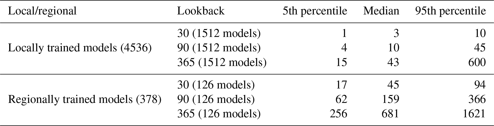
Statistics of the wall-clock time spent to train each one of the LSTM models are summarized in Table B1. We trained a total of 4536 local models (18 loss functions, 4 input variables, 3 lookbacks, and 21 stations) and 378 regional models (18 loss functions, 7 input variables, 3 lookbacks) on three computing units with distinct CPU cores (Intel^® Xeon^® W-2265 with base frequency at 3.5 GHz, Intel^® Xeon^® W3-2425 with base frequency at 3.0 GHz, and Intel^® Xeon^® Silver 4216 with base frequency at 2.1 GHz). At each computing unit, we set the number of threads dedicated to each model training at 7. Note that the training was halted once a plateau in the validation performances was reached (100 epochs without a decrease in MSE by 0.001 °C²). Table B1 shows that the training time increases at leading order with the lookback and the amount of data used for training (local vs. regional training). Training a local model takes from ∼3 min (median value) for a lookback of 30 d up to ∼45 min (median value) for a lookback of 365 d. Training a regional model takes from ∼45 min (median value) for a lookback of 30 d and up to ∼12 h (median value) for a lookback of 365 d.

Table B1 Statistics of the wall-clock time (in min) needed for the training of the local and regional LSTM models. The number of models from which the statistics were computed is specified between brackets for each training strategy and each lookback.

Appendix C: Test performances using RMSE

To control whether the choice of MAE as an evaluation metric biases the results in favour of MAE-based loss functions, and in order to compare our results with previous studies (e.g., Rahmani et al., 2021a), we also evaluated the test performances using RMSE as a criterion. Figure C1 shows the evolution of the test performances with respect to the choice of the loss function, and comparing it with Fig. 2 suggests that using MAE as a criterion for test performances does not bias our conclusions in favour of MAE-based loss functions (see the results with local models, Fig. C1a). Figures C2 and C3 show the performances of the locally trained (Fig. C2) and the regionally trained (Fig. C3) LSTM models, which are replicates of Figs. 3 and 4 but with RMSE instead of MAE as an evaluation metric. These figures confirm the importance of regional training with catchment attributes in improving the LSTM performances especially for the range of extreme (top 10 %) T_w values.

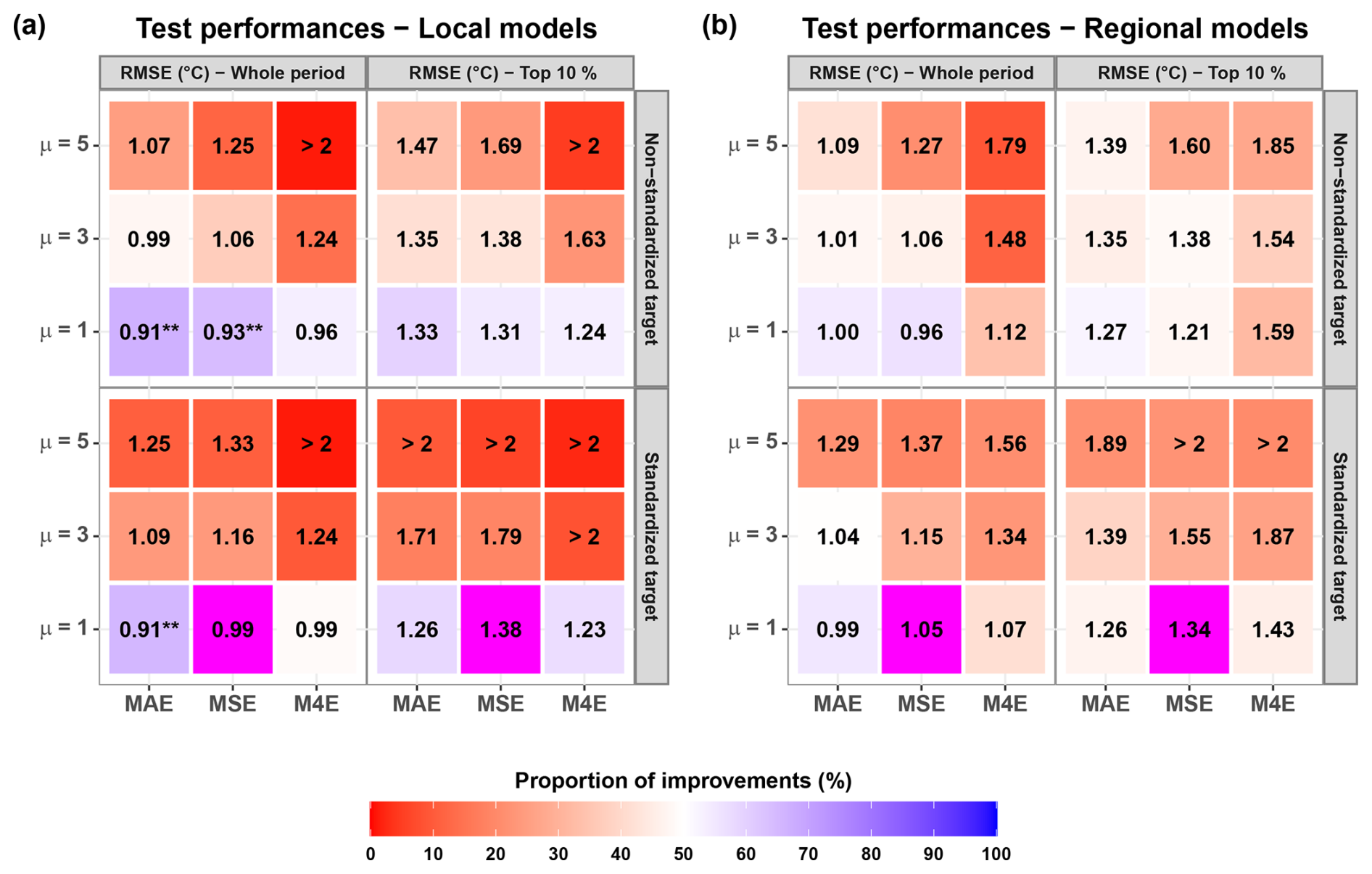
Figure C1 Median test performances (RMSE, in °C) of the local models (a) and the regional models (b) according to the loss function used for training. This figure is similar to Fig. 2 but with RMSE as a criterion to evaluate the test performances. Colours indicate the proportion of cases for which the use of the loss function yielded better results than the reference loss function (MSE with standardization, shown in magenta). Asterisks indicate that the custom loss function is significantly better than the reference loss function according to the one-sided binomial test: * for a significance threshold of 5 %, ** for a threshold of 1 %, and *** for a threshold of 0.1 %.

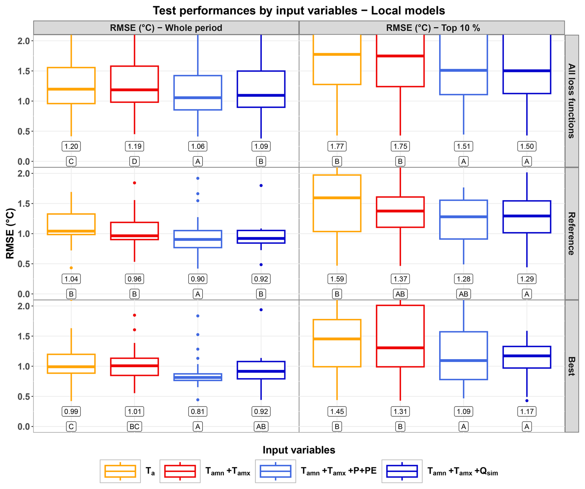
Figure C2 Distributions of the test performances (RMSE, in °C) of the local models over the whole test period (left column) and the test subperiod corresponding to the highest 10 % observed values (right column). This figure is similar to Fig. 3 but with RMSE as a criterion to evaluate the test performances. The top row shows the distribution over all the loss functions ($\mathrm{18}\times \mathrm{21}=\mathrm{378}$ points per distribution). The middle row shows the performances for the reference loss function (MSE with standardization, 21 points per distribution). The bottom row shows the performances for the best loss function over all sets of input variables (MAE without standardization for the whole period and M4E with standardization for the top 10 %, 21 points per distribution). Numerical values under the boxes represent the median value for each distribution. Letters under the numerical values rank the distributions, and are defined such as distributions that share at least one letter are not significantly different according to the one-sided binomial test. Note that the models we kept for test do not necessarily share the same lookback.

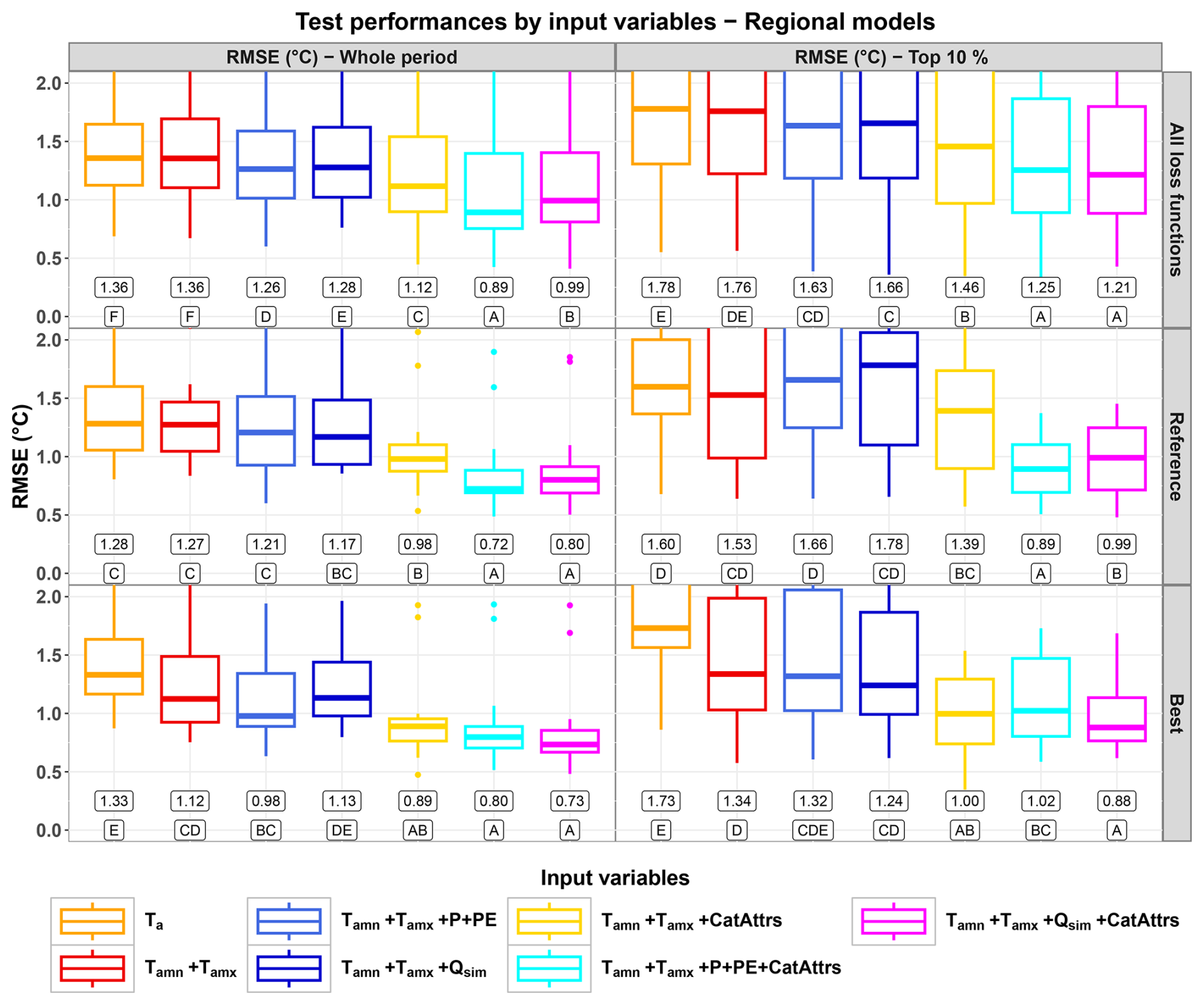
Figure C3 Distributions of the test performances (RMSE, in °C) of the regionally trained models over the whole test period (left column) and the test subperiod corresponding to the highest 10 % observed values (right column). This figure is similar to Fig. 4 but with RMSE as a criterion to evaluate the test performances. Top row shows the distribution over all the loss functions ($\mathrm{18}\times \mathrm{21}=\mathrm{378}$ points per distribution). The middle row shows the performances for the reference loss function (MSE with standardization, 21 points per distribution). The bottom row shows the performances with the best loss function over all sets of input variables (MSE without standardization for both cases). Numerical values under the boxes represent the median value for each distribution. Letters under the numerical values rank the distributions, and are defined such as distributions that share at least one letter are not significantly different according to the one-sided binomial test. Note that the models we kept for test do not necessarily share the same lookback.