Comprehensive Global Assessment of 24 Gridded Precipitation Datasets Across 18 428 Catchments Using Hydrological Modeling

Numerous gridded precipitation (P) datasets have been developed to address a variety of needs and challenges. However, selecting the most suitable and reliable dataset remains difficult for users. We conducted the most comprehensive global evaluation to date of gridded (sub-)daily P datasets using hydrological modeling. A total of 24 datasets – derived from satellite, (re)analysis, gauge sources, or combinations thereof – were assessed. To evaluate their performance, we calibrated the conceptual hydrological model HBV against observed daily streamflow for 18 428 catchments (each <10 000 km²) worldwide, using each P dataset as input. The Kling-Gupta Efficiency (KGE) was used as performance metric, with the calibration score serving as proxy for P dataset performance. Overall, Multi-Source Weighted-Ensemble Precipitation (MSWEP) V2.8 demonstrated the best performance (median KGE of 0.78), highlighting the value of merging P estimates from diverse data sources and applying daily gauge corrections. Among the purely satellite-based P datasets, the soil moisture- and microwave-based Global Precipitation Mission plus Soil Moisture to RAIN (GPM + SM2RAIN) dataset performed best (median KGE of 0.64). The Global Data Assimilation System (GDAS) analysis ranked highest among the (re)analyses (median KGE of 0.72), slightly outperforming the widely used European Centre for Medium-range Weather Forecasts ReAnalysis 5 (ERA5; median KGE of 0.71). Performance varied across Köppen-Geiger climate zones, with the highest scores in polar (E) regions (median KGE of 0.76 across datasets) and the lowest in arid (B) regions (median KGE of 0.53 across datasets). Spatial correlation analysis between catchment attributes and KGE scores identified aridity index, potential evaporation, and P occurrence as the strongest predictors of performance. Our assessment revealed significant regional differences in dataset performance and error characteristics, emphasizing the importance of careful dataset selection for water resource management, hazard assessment, agricultural planning, and environmental monitoring.

1 Introduction

Understanding the spatio-temporal distribution of precipitation (P) is crucial for a wide range of applications, including water resources assessment, flood forecasting, agricultural monitoring, and disease tracking (Dresel et al., 2018; Liang and Gornish, 2019; McKinnon and Deser, 2021; Hinge et al., 2022; Dimitrova et al., 2022). However, P exhibits high variability across space and time, making it difficult to estimate, particularly in regions with complex topography, convection-driven P, or snow-dominated climates (Herold et al., 2016; Prein and Gobiet, 2017; Sharma et al., 2020b; Li et al., 2020; Tarek et al., 2021). P estimates can be derived from satellites, models, and rain gauges, but each data source is subject to limitations. Satellite retrievals are hindered by surface snow and ice contamination (Cao et al., 2018; Chen et al., 2020), struggle to capture shallow orographic P (Yamamoto et al., 2017; Adhikari and Behrangi, 2022), and face challenges in detecting snowfall (You et al., 2021; Jääskeläinen et al., 2024; Girotto et al., 2024b). Reanalyses (e.g., European Centre for Medium-range Weather Forecasts ReAnalysis 5 – ERA5; Hersbach et al., 2020) rely on uncertain parameterizations and often lack sufficient spatial resolution to adequately capture orographic effects (Skamarock, 2004; Ménégoz et al., 2013; Liu et al., 2018). Rain gauge networks are sparse and biased towards lower elevations (Schneider et al., 2014; Kidd et al., 2017; Ehsani and Behrangi, 2022) and gauges can severely underestimate snowfall due to wind-induced under-catch (Groisman and Legates, 1994; Sevruk et al., 2009; Rasmussen et al., 2012; Girotto et al., 2024a).

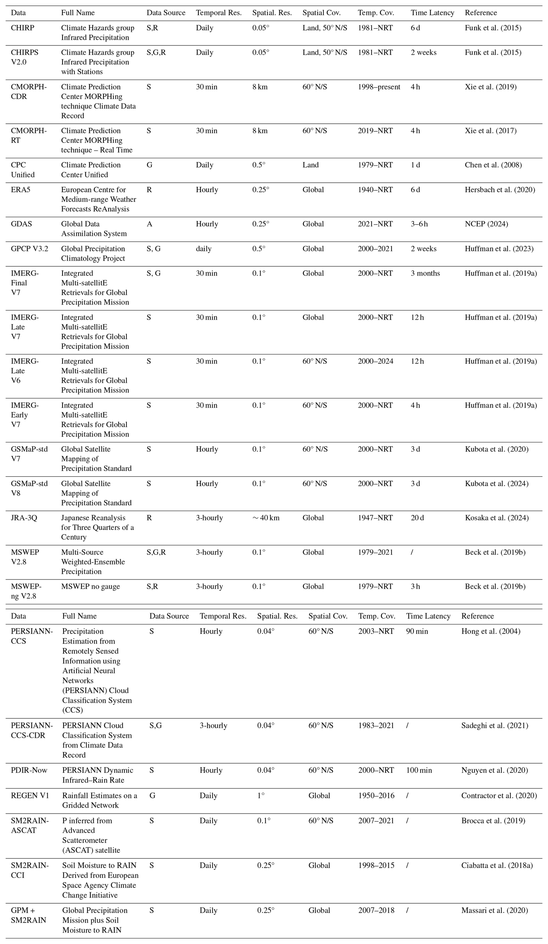
In recent decades, numerous gridded P datasets have been developed based on these data sources and combinations thereof. Each dataset has a different design objectives, spatio-temporal resolution, coverage, algorithms, and latency (see Table 1 for an overview of quasi- and fully-global datasets). A plethora of studies have evaluated these datasets (see, e.g., reviews by Gebremichael, 2010; Maggioni et al., 2016, and Sun et al., 2018). However, the large majority of these studies use rain gauge observations as reference, which has limitations: (i) rain gauge observations are unavailable in many regions (Kidd et al., 2017); (ii) differences in scale between point-based rain gauges and grid-based P datasets (Ensor and Robeson, 2008; Yates et al., 2006) can skew results; (iii) time discrepancies between daily accumulations of gauges and satellite and (re)analysis datasets (Yang et al., 2020; Beck et al., 2019b) can yield misleading daily evaluation results; (iv) the systematic P underestimation by rain gauges in snow-dominated and mountainous regions (Groisman and Legates, 1994; Sevruk et al., 2009; Rasmussen et al., 2012) can unfairly penalize P datasets in these regions; and (iv) using rain gauges already incorporated into the P datasets for validation results in misleading conclusions.

An alternative approach to evaluate P datasets is to use hydrological modeling, wherein streamflow simulations driven by different P datasets are compared to streamflow observations. The degree of correspondence between simulated and observed streamflow serves as a proxy for how accurately the P dataset captures the intensity and timing of P events. This approach avoids the aforementioned limitations by providing a direct, real-world measure of performance that reflects the dataset's ability to capture P dynamics in a hydrological context (Camici et al., 2018). Several studies have successfully employed this approach to evaluate various P datasets (e.g., Voisin et al., 2008; Su et al., 2008; Bitew et al., 2012; Tang et al., 2016; Beck et al., 2017c; Lussana et al., 2018; Mazzoleni et al., 2019; Pradhan and Indu, 2021; Xiang et al., 2021; Gu et al., 2023; Gebrechorkos et al., 2023). However, many studies are limited in scope by (i) focusing on specific regions or subcontinents, or using streamflow data from relatively few catchments, thus restricting the generalizability of their findings; (ii) analyzing only a small subset of available P datasets, often excluding (re)analysis-based datasets; (iii) focusing on a monthly rather than daily time scale, which can obscure important short-term variability, such as extreme rainfall events or floods. Additionally, several studies failed to re-calibrate the hydrological model for each P dataset, including the recent global assessment by Gebrechorkos et al. (2023), which could result in biased conclusions.

In this study, we present the most comprehensive evaluation to date of gridded (sub-)daily (quasi-)global P datasets, aiming to identify their strengths and limitations across diverse geographical and climatological settings, and to inform their suitability for hydrological applications. We leverage an unparalleled database of streamflow observations from 18,428 catchments worldwide, spanning all climate zones and latitudes, to ensure broad generalizability of our results. Moreover, we evaluate an extensive collection of 24 P datasets, including new datasets like the microwave-based IMERG V7 (Huffman et al., 2019b), the infrared-based PDIR-Now (Nguyen et al., 2020), and the reanalysis JRA-3Q (Kosaka et al., 2024), all three of which have not been comprehensively assessed at the global scale yet. To provide a fair and balanced assessment, we re-calibrate the hydrological model for each P dataset.

2 Data and Methods

2.1 Gridded P Datasets

Table 1 lists the 24 gridded P datasets included in our assessment. These datasets were selected based on their global or quasi-global coverage, widespread use in hydrological applications, and availability of daily or sub-daily data. Regional datasets, while valuable, were excluded to maintain consistency across diverse geographic areas (e.g., Asian Precipitation - Highly-Resolved Observational Data Integration Towards Evaluation – APHRODITE, Yatagai et al., 2012, and North American Land Data Assimilation System – NLDAS, Xia et al., 2012). The selected datasets are tailored for specific purposes: some, like IMERG-Early V7 and PDIR-Now, are designed for short-latency applications such as near-real-time monitoring heavy P events, while others with longer latency, such as CHIRPS V2.0 and IMERG-Final V7, are more suitable for comprehensive, long-term climate and hydrological analyses.

The 24 P datasets are grouped into six categories based on their input data sources (see Table 1 for full dataset names and references): (i) Satellite-only (S): IMERG-Early V7, IMERG-Late V6, IMERG-Late V7, PERSIANN-CCS, PDIR-Now, GSMaP-std V7, GSMaP-std V8, SM2RAIN-ASCAT, SM2RAIN-CCI, GPM + SM2RAIN, CMORPH-CDR, and CMORPH-RT; (ii) Reanalysis- or Analysis-only (R/A): ERA5, GDAS, and JRA-3Q; (iii) Gauge-only (G): CPC Unified and REGEN V1; (iv) Satellite and Gauge (S + G): IMERG-Final V7, GPCP V3.2, and PERSIANN-CCS-CDR; (v) Satellite, Reanalysis, and Gauge (S + R + G): CHIRPS V2.0, MSWEP V2.8; and (vi) Satellite and Reanalysis (S + R): CHIRP, MSWEP-ng V2.8. Version numbers are consistently indicated throughout the manuscript to ensure transparency and reproducibility.

Funk et al. (2015)Funk et al. (2015)Xie et al. (2019)Xie et al. (2017)Chen et al. (2008)Hersbach et al. (2020)NCEP (2024)Huffman et al. (2023)Huffman et al. (2019a)Huffman et al. (2019a)Huffman et al. (2019a)Huffman et al. (2019a)Kubota et al. (2020)Kubota et al. (2024)Kosaka et al. (2024)Beck et al. (2019b)Beck et al. (2019b)Hong et al. (2004)Sadeghi et al. (2021)Nguyen et al. (2020)Contractor et al. (2020)Brocca et al. (2019)Ciabatta et al. (2018a)Massari et al. (2020)

Table 1 Overview of the (sub-)daily (quasi-)global gridded P datasets evaluated in this study. Definition of abbreviations: S: satellite, G: gauge, R: Reanalysis, A: Analysis, and NRT: near real time.

2.2 Streamflow Observations and Catchment Selection

We utilized a comprehensive global database of daily streamflow observations and catchment boundaries compiled from 29 national and international datasets. Appendix A provides a detailed list of the data sources, along with corresponding references or websites. Initially, the database contained 43 627 stations. However, as many stations appeared in multiple data sources, we performed a duplication check and discarded stations where both the station location and the corresponding catchment centroid were within 5 km of those of another station. In case of duplication, regional data sources were prioritized over international ones (e.g., CAMELS datasets were preferred over GRDC). After this process, the number of unique stations was reduced to 35 254.

To ensure the suitability of the catchments for the present analysis, we applied the following inclusion criteria:

1. Catchment areas were limited to <10 000 km² to minimize the influence of channel routing, which can become significant at the daily time scale in larger catchments (Gericke and Smithers, 2014). Moreover, since we use catchment-mean P time series to drive the hydrological model, larger catchments are prone to greater spatial averaging, leading to a less realistic representation of P patterns.

2. The total streamflow record had to be >3 years, not necessarily consecutive. This threshold was chosen due to the short records of GDAS and CMORPH-RT. We realize that such a short record may introduce some random variability in the KGE scores of these datasets, particularly in arid regions where P events are less frequent. However, this random variability will likely be averaged out due to the large number of catchments included in our assessment.

3. The number of days with appreciable runoff (>5 mm d⁻¹) had to exceed 10, and these days could not be consecutive (i.e., they should not be part of a single continuous event). This ensures that the calibration is based on a sufficient number of distinct runoff events.

4. The mean annual runoff had to be ≥5 and <5000 mm yr⁻¹, to filter out catchments with erroneous streamflow and/or catchment boundary data.

5. The reservoir influence (defined as the ratio of total reservoir capacity to mean cumulative annual streamflow) had to be <0.1, as Hydrologiska Byråns Vattenbalansavdelning (HBV), the hydrological model used in this study, does not explicitly simulate reservoirs. To determine the total reservoir capacity, we used the Global Reservoir and Dam (GRanD) dataset (V1.3; Lehner et al., 2011).

After applying these criteria, 18 428 catchments remained. The 2.5th, 10th, 50th, 90th and 97.5th percentiles of the catchment areas are 23, 55, 213, 2688 and 6165 km², respectively (Fig. 1).

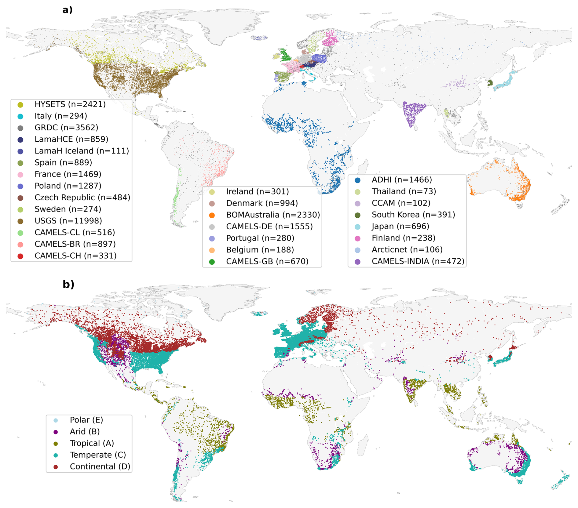
Figure 1 Locations of the 35 254 gauges with daily streamflow data that passed the duplication checks, used to evaluate the gridded P datasets. Each data point represents the centroid of a catchment. The colors indicates the dominant major Köppen-Geiger climate class, based on the 1 km resolution map for 1991–2020 from Beck et al. (2023). For more information on the streamflow data sources, refer to Appendix A.

2.3 Hydrological Modeling

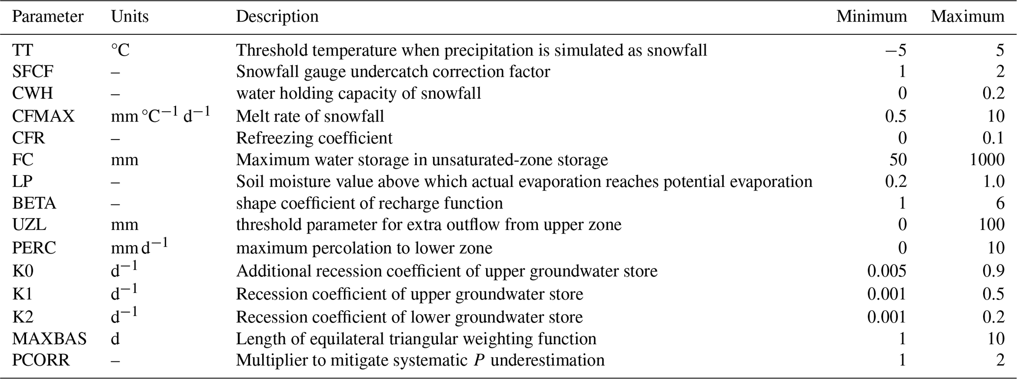
The performance of the gridded P datasets was assessed using hydrological modeling for the 18,428 catchments that passed the suitability checks. For each catchment, the HBV conceptual hydrological model (Bergström, 1992; Seibert and Vis, 2012) was calibrated against daily streamflow observations using time series from each P dataset. The HBV model was selected due to its versatility and computational efficiency, and numerous successful applications (see review by Seibert and Bergström, 2022). The model incorporates two groundwater stores, one unsaturated-zone store, and a triangular weighting function to simulate channel routing delays. Table 2 provides the model parameters and their calibration ranges. An additional parameter, PCORR, was introduced to further adjust for systematic P biases, which are generally easier to mitigate and should, therefore, not disproportionately penalize the datasets. Note that PCORR and SFCF are applied simultaneously: SFCF adjusts snowfall for gauge undercatch, while PCORR scales total P. Snowfall is therefore affected by both.

Table 2 HBV model parameter descriptions and calibration ranges.

The model requires daily time series of P, potential evaporation, and air temperature as inputs. We used catchment-mean daily P time series from the gridded datasets listed in Table 1. Daily potential evaporation was estimated using the Penman-Monteith equation (Penman, 1948; Monteith, 1965), which requires daily time series of air temperature, downward shortwave and longwave radiation, relative humidity, and wind speed as input. Catchment-mean daily time series of these variables were sourced from the Multi-Source Weather (MSWX) dataset (Beck et al., 2022). MSWX improves on ERA5 by providing bias-adjusted fields at 0.1° resolution. The finer grid better captures mountain gradients that govern snowfall and snowmelt.

2.4 Calibration Procedure

The 15 model parameters were calibrated for each catchment and P dataset over the period where both observed streamflow and P data were available. Model initialization was done by running the model with 10 years of prior P data, if available. If 10 years of prior P data were not available, the model was run multiple times using the available P data until a total of more than 10 years was accumulated. Furthermore, simulation of 365 d was not used for calculating model performance. We used a (μ+λ) evolutionary algorithm, which is a population-based optimization method that iteratively evolves solutions through selection, crossover, and mutation to maximize the Kling-Gupta Efficiency (KGE) objective. The algorithm was implemented using the Distributed Evolutionary Algorithms in Python (DEAP) library (version 1.4; Ashlock, 2010; Fortin et al., 2012), with a population size (μ) of 20 and an offspring pool size (λ) of 48. Crossover was applied with a probability of 90 %, and mutation was applied with a probability of 10 % using a Gaussian-based mutation operator. To ensure convergence, the optimization process was terminated if the best KGE value did not improve by more than 0.01 for five consecutive generations after a minimum of 25 generations.

To assess the influence of systematic P bias correction using the PCORR and SFCF adjustment factors on model performance, we explored four calibration scenarios with varying bounds for the PCORR and SFCF parameters. In the first scenario, PCORR was allowed to vary between 0.0 and 2.0, providing full flexibility to adjust for both under- and overestimation of P, while SFCF was allowed to vary between 1.0 to 2.0. The second scenario limited PCORR to the range 0.5–2.0, while keeping the range of SFCF between 1.0 and 2.0. The third scenario fixed both PCORR and SFCF parameters at 1.0, effectively disabling P bias correction. The fourth scenario constrained both PCORR and SFCF to the range 1.0–2.0, allowing only upward correction. These scenarios enabled us to evaluate the sensitivity of model performance to P bias correction and assess the robustness of P dataset rankings under varying calibration constraints.

In line with several previous studies (e.g., Beck et al., 2017c; Tarek et al., 2020; Arsenault et al., 2023), we opted not to split the record into separate calibration and validation periods. Instead, the full period of overlapping streamflow and P data was used to maximize the available information for parameter calibration and evaluation and yield more reliable scores. This is particularly critical for P datasets with short records (GDAS and CMORPH-RT), where splitting the data would lead to scores based on only one or two years of data which could cause instability in the performance scores (see Arsenault et al., 2018).

2.5 Performance Metric

To assess the performance of streamflow simulations forced by the different gridded P datasets, we calculated the Kling-Gupta Efficiency (KGE) scores between daily observed and simulated streamflow for each catchment. KGE, introduced by Gupta et al. (2009) and modified by Kling et al. (2012), is an objective performance metric that combines correlation, bias, and variability, and is defined as:

$$\begin{array}{}\text{(1)}& \text{KGE}=\mathrm{1}-\sqrt{{\left(r-\mathrm{1}\right)}^{\mathrm{2}}+{\left(\mathit{\gamma }-\mathrm{1}\right)}^{\mathrm{2}}+{\left(\mathit{\beta }-\mathrm{1}\right)}^{\mathrm{2}}},\end{array}$$

where r represents the Pearson correlation coefficient, γ is the ratio of the estimated to observed coefficients of variation, and β is the ratio of estimated to observed means:

$$\begin{array}{}\text{(2)}& \mathit{\gamma }={\displaystyle \frac{{\mathit{\sigma }}_{\mathrm{s}}/{\mathit{\mu }}_{\mathrm{s}}}{{\mathit{\sigma }}_{\mathrm{o}}/{\mathit{\mu }}_{\mathrm{o}}}},\mathit{\beta }={\displaystyle \frac{{\mathit{\mu }}_{\mathrm{s}}}{{\mathit{\mu }}_{\mathrm{o}}}},\end{array}$$

where μ and σ are the mean and standard deviation, respectively, and the subscripts “s” and “o” refer to the estimated and observed values. Optimal values for KGE, r, β, and γ are all 1. The r term is primarily sensitive to the timing and intensity of P extremes, while β captures systematic over- or underestimation of P. While the PCORR and SFCF parameters, which account for systematic biases, were calibrated, the β component of KGE reflects residual biases that may persist due to limitations in the P dataset's ability to accurately represent the spatial and temporal distribution of P intensities and magnitudes (Sun et al., 2018).

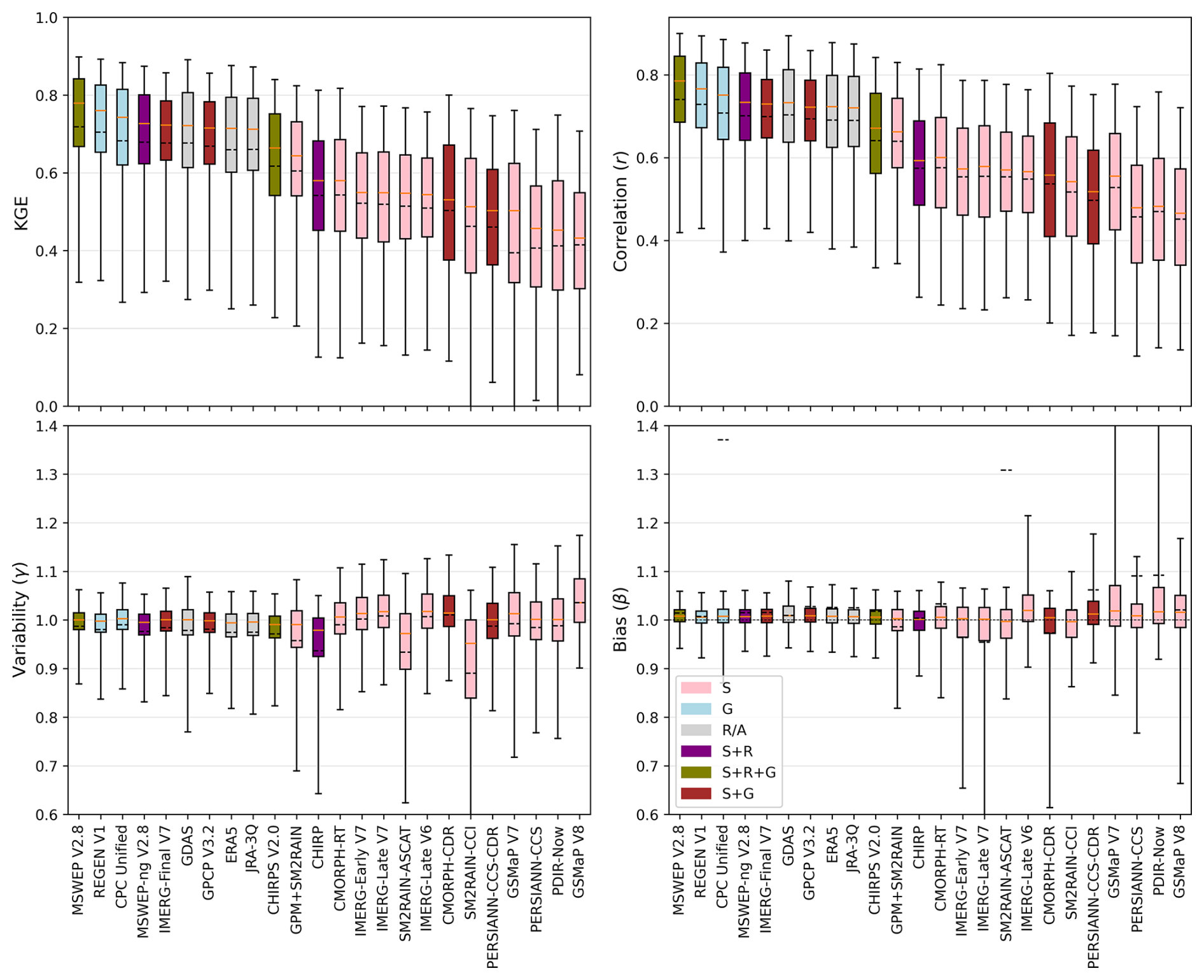
Figure 2 Calibration KGE, correlation (r), long-term bias (β), and variability ratio (γ) scores achieved by the 24 P datasets. For a given catchment, calibration periods were not necessarily consistent across P datasets because their temporal coverage differs. The horizontal black and orange lines represent the mean and median, respectively. The box extends from the 25th to 75th percentiles, while the whiskers represent the 5th and 95th percentiles. The datasets are sorted according to their median KGE values. The colors represent the dataset type: S: Satellite; G: Gauge; R/A: Reanalysis or Analysis; S + R: Satellite and Reanalysis; S + R + G: Satellite, Reanalysis, and Gauge; and S + G: Satellite and Gauge.

3 Results and Discussion

3.1 Overall Model Performance

Figure 2 presents median calibration scores obtained by HBV forced with 24 gridded P datasets across 18 428 catchments. Figure 3 maps the best-performing P dataset in each catchment, restricted to the five datasets with the highest median KGE for clarity. The key findings are as follows:

• Among the six main categories of P datasets – satellite, gauge, (re)analysis, satellite+reanalysis, satellite + reanalysis + gauge, and satellite + gauge – the satellite category performed the worst overall. This challenges the common misconception that satellite datasets are inherently superior due to their high spatial resolution and observational nature. However, (re)analyses are also “observation-based”, as they assimilate vast quantities of satellite, surface, radiosonde, and aircraft data. Furthermore, our results indicate that higher spatial resolution does not necessarily guarantee better performance, though this may be because P data are spatially averaged at the catchment scale. Nonetheless, that satellite P datasets underperform globally should not be interpreted as a lack of value; for instance, they excel in tropical regions, as will be discussed in Sect. 3.2.

• The multi-source MSWEP V2.8 dataset (Beck et al., 2019b) attains the highest overall performance, with a median KGE of 0.78 (the spatial distribution of KGE values is provided in Fig. S1 in the Supplement). This dataset leverages the complementary strengths of gauge, satellite, and (re)analysis data to provide improved P estimates across the globe. Specifically, daily gauge observations enhance performance in regions with dense rain gauge networks, satellite retrievals enhance performance in convection-dominated regions and periods, while (re)analysis outputs improve performance in frontal-dominated regions and periods (Beck et al., 2019b).

• Among the purely satellite-based P datasets (CMORPH-CDR and -RT; IMERG-Early and -Late; GSMaP; PDIR-Now; PERSIANN-CCS; and SM2RAIN-ASCAT and -CCI; and GPM + SM2RAIN), the GPM + SM2RAIN dataset (Massari et al., 2020) exhibited the best overall performance (median KGE of 0.64; Fig. 2). This dataset combines satellite soil moisture retrievals from ASCAT H113 H-SAF, SMOS L3 and SMAP L3 with microwave-based P retrievals from IMERG using the so-called optimal linear combination approach (Bishop and Abramowitz, 2013). IMERG-Late V7 (median KGE of 0.55) introduced several improvements over V6, notably a climatological rain gauge adjustment, leading to a slight performance boost compared to V6 (median KGE of 0.54), particularly in the tropical, cold, and polar catchments (Fig. S14). In contrast, GSMaP-std V8 (median KGE of 0.43) performed worse than its predecessor, GSMaP-std V7 (median KGE of 0.50).

• Among the purely infrared-based P datasets (PERSIANN-CCS and PDIR-Now), PERSIANN-CCS (Hong et al., 2004; median KGE of 0.46) performed similar to PDIR-Now (Nguyen et al., 2020; median KGE of 0.45). This is surprising as PDIR-Now features several improvements over PERSIANN-CCS, such as the dynamic adjustment of the relationship between cloud-top brightness temperatures and rain rates based on rainfall climatologies, as well as the use of a higher temperature threshold to enhance the detection of warm rain events (Nguyen et al., 2020). Further analysis revealed that PDIR-Now performs particularly poorly in the UK, Denmark, and Italy (Fig. S27), resulting in its overall poorer performance compared to PERSIANN-CCS.

• Among the (re)analyses (ERA5, GDAS, and JRA-3Q), GDAS, based on V16.3 from 2022 of the Global Forecasting System (GFS) model (http://www.ncei.noaa.gov/products/weather-climate-models/global-forecast, last access: 5 May 2026), performed best (median KGE of 0.72). The recently released reanalysis JRA-3Q, based on the Japan Meteorological Agency (JMA) operational system as of December 2018 (Kosaka et al., 2024), performed similarly to ERA5 (both yielding a median KGE of 0.71). ERA5 is based on Cycle 41r2 of the Integrated Forecasting System (IFS) model from 2016 (Hersbach et al., 2020). While ERA5 is widely regarded as the most reliable reanalysis overall, these results suggest that JRA-3Q is a viable alternative for hydrological modeling. GDAS has a much shorter record than ERA5 and JRA-3Q (Table 1), which limits its usefulness.

• Among the rain gauge-based P datasets (CHIRPS 2.0, CPC Unified, GPCP V3.2, IMERG-Final V7, MSWEP V2.8, REGEN V1, and PERSIANN-CCS-CDR), MSWEP V2.8 (Beck et al., 2019b) achieved the best overall performance (median KGE of 0.78), underscoring the value of combining P estimates from satellite, reanalysis, and gauge data and applying daily gauge corrections. In contrast, CHIRPS V2.0 (median KGE of 0.66) applies 5 d gauge corrections, while the other datasets apply monthly corrections, which provide fewer benefits at the daily time scale. The main challenge in applying daily gauge corrections is accounting for offsets in daily gauge reporting times, as accumulations rarely align with midnight UTC (Yang et al., 2020). Furthermore, daily correction efforts are often hindered by the sparsity of gauge networks outside North America, Europe, and Australia (Kidd et al., 2017). Because CPC Unified and REGEN V1 rely exclusively on daily gauge observations, their performance is limited in these data-sparse regions, where values are interpolated between distant gauges (Fig. S29).

• The marked differences in median KGE values between MSWEP V2.8 and MSWEP-ng V2.8 (median KGE of 0.78 vs. 0.73), between CHIRPS V2.0 and CHIRP (median KGE of 0.66 vs. 0.58), and between IMERG-Final V7 and -Late V7 (median KGE of 0.72 vs. 0.55) emphasize the importance of applying gauge corrections, in line with previous evaluations (Gochis et al., 2009; Beck et al., 2017c, b; Shen et al., 2018). This highlights the critical role national meteorological agencies play in feeding rain gauge data into global databases such as the Global Historical Climatology Network daily (GHCNd; Menne et al., 2012) and the need to expand gauge coverage and promote open data sharing, particularly in data-scarce regions, to improve the utility of P datasets in those areas.

• Our results reaffirm that higher-resolution P datasets do not necessarily yield better streamflow simulations compared to lower-resolution datasets, consistent with previous assessments (e.g., Bador et al., 2020; Huang et al., 2019; Chan et al., 2013). Notably, the 0.04° resolution satellite infrared-based datasets (PERSIANN-CCS and -CCS-CDR, and PDIR-Now; median KGE of 0.46, 0.50, and 0.45, respectively) – the highest resolution datasets included in our assessment – do not consistently perform better neither globally nor for any Köppen-Geiger climate zone, although this may reflect the generally poor performance of infrared-based datasets. However, IMERG-Final V7 (0.1° resolution) also does not perform better than GPCP V3.2 (0.5° resolution), which uses IMERG for disaggregation from monthly to daily. This may at least partly be due to the use of catchment-mean P to drive HBV, which omits local variability that high-resolution datasets might otherwise capture. Another potential factor is that coarser datasets may inadvertently improve reliability by averaging out small-scale random errors; however, our catchment-scale assessment cannot confirm this. Conversely, for the (re)analyses, the benefits of a higher resolution are evident in mountainous regions. Here, the 13 km GDAS outperformed the 31 km ERA5, which in turn outperformed the 40 km JRA-3Q (Fig. S57; see also Sect. 3.2). This indicates that higher-resolution NWP models are, as expected, more capable of accurately capturing complex orographic P dynamics.

• A comparison of PCORR parameter values obtained after calibration using different P datasets reveals that IMERG-Early and -Late V7 necessitate the highest PCORR values, while PDIR-Now requires the lowest values (Figs. S3–S26). The lower PCORR for PDIR-Now reflects its tendency to overestimate P, as confirmed by the significant positive bias obtained by the datasets (Fig. 2). This may be because the algorithm was calibrated with a focus on heavy rainfall events for near real-time applications (Nguyen et al., 2020). Conversely, the higher PCORR values required for IMERG-Early and -Late V7 reflect their tendency to underestimate P, which is confirmed by their lower bias values (Fig. 2).

• The overall ranking of P datasets remained largely consistent across the four PCORR calibration scenarios (Fig. S30; see Sect. 2.4). However, in the scenario where PCORR and SFCF were fixed at 1.0, GPCP V3.2 and ERA5 showed improved relative rankings – not due to higher performance, but because other datasets experienced greater performance drops under this constraint. Most datasets showed little sensitivity to the PCORR bound below 1.0, but a few – namely PDIR-Now, GSMaP V7, PERSIANN-CCS-CDR, and IMERG-Late V6 – exhibited notable use of PCORR values below 1.0 (Fig. S31). This suggests that these datasets tend to overestimate P, and that downward rescaling improves their hydrological performance.

• The lower performance of PDIR-Now can be partially attributed to the default PCORR range of 1.0–2.0, which precludes the correction of P overestimation. This is confirmed by the lower calibrated PCORR values when allowed to vary below 1.0, leading to a decrease in the median calibrated PCORR from 1.2 to 1.1 and a marked improvement in median KGE from 0.43 to 0.47. Further analysis showed that the largest decrease in median calibrated PCORR (from 1.0 to 0.7) and corresponding improvement in KGE (from 0.15 to 0.37) occurred in CAMELS-GB (Fig. S33). However, across most other P datasets, the improvement in KGE was negligible when PCORR was allowed to drop below 1.0, confirming that the default PCORR range (1.0–2.0) is appropriate for most P datasets (Fig. S32).

• We found that several satellite P datasets (notably IMERG-Early and -Late V7, SM2RAIN-ASCAT, SM2RAIN-CCI, GSMaP V8, and CMORPH-CDR) exhibit pronounced low-β tails (Fig. 2), indicating significant local P underestimation. This finding is further corroborated by maps of the difference between the mean annual P of each product and the multi-product mean (Figs. S34–S56), revealing extensive regions with negative values.

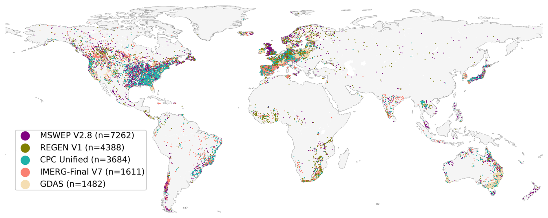
Figure 3 Precipitation (P) dataset with the highest calibration KGE in each catchment. Points mark catchment centroids (n=18 428). For clarity, only the five datasets with the highest median KGE are shown. MSWEP-np V2.8 is omitted because it is highly similar to MSWEP V2.8.

Overall, our findings align with those of Beck et al. (2017c), Gu et al. (2023), and Gebrechorkos et al. (2023), who similarly evaluated multiple gridded P datasets using hydrological modeling in catchments worldwide. However, while Beck et al. (2017c) assessed nine datasets across 9053 catchments, Gu et al. (2023) evaluated two datasets across 10 596 catchments, and Gebrechorkos et al. (2023) analyzed six datasets across 1825 catchments, the present study evaluates 24 datasets across 18 428 catchments. This broader scope significantly enhances the generalizability of our results. Additionally, Beck et al. (2017c) and Gu et al. (2023) primarily assessed outdated versions of P datasets, whereas our analysis includes several new P datasets – such as PDIR-Now, IMERG V7, JRA-3Q, and MSWEP V2.8 – that have not yet been comprehensively evaluated. Furthermore, unlike Gebrechorkos et al. (2023), we recalibrated the hydrological model for each P dataset, reducing the risk of penalizing datasets for systematic biases that calibration can otherwise absorb.

3.2 Regional Performance Differences

Table 3 presents median calibration KGE scores for the 24 gridded P datasets across the five major Köppen-Geiger climate classes (see Fig. S2 for the distribution of KGE values). While satellite P datasets perform the worst overall (see Sect. 3.1), microwave-based satellite datasets such as IMERG and GSMaP generally outperform (re)analyses (ERA5, GDAS, and JRA-3Q) in tropical catchments. This is likely because tropical P events, typically localized and short-lived, can be directly observed by satellites, while numerical weather prediction (NWP) models generally struggle to simulate the complex convective processes driving these events (Yano et al., 2018; Peters et al., 2019; Lin et al., 2022). Conversely, in temperate and, most notably, cold regions, (re)analyses generally outperform satellite-based datasets. This is because the large-scale, long-duration frontal P systems dominant in these regions are reliably simulated by NWP models (Ebert et al., 2007; Beck et al., 2017c, 2019a; Sun et al., 2018). In arid climates, all P datasets tend to perform relatively poorly, with a slight advantage for (re)analyses over satellite-based datasets, consistent with previous evaluation (e.g., Beck et al., 2017a, 2016). The lower arid-region scores mainly reflect (i) poorer forcing quality due to the short-lived, localized nature of storms and sub-cloud evaporation (virga) (Wang et al., 2018); (ii) more threshold-driven runoff generation that amplifies small forcing errors; and (iii) fewer runoff-producing events, which increases sampling uncertainty (Beck et al., 2017a, c; Sun et al., 2018; El Kenawy et al., 2019; Beck et al., 2019a; Williams, 2025). Thus, the lower performance does not necessarily indicate an inability of HBV to represent arid hydrology.

Table 3 Median daily calibration KGE values obtained using HBV driven by the different P datasets for all catchments and the five major Köppen-Geiger climate classes. For the Köppen–Geiger classes, medians are omitted when a dataset has <100 catchments or covers <50 % of the catchments in that class. In each column, the dataset with the best performance is shown in bold. The catchments were classified based on the most dominant class, determined using the 1 km resolution Köppen-Geiger map for 1991–2020 from Beck et al. (2023). See Fig. 1 for a map of the dominant major Köppen-Geiger climate class for the catchments.

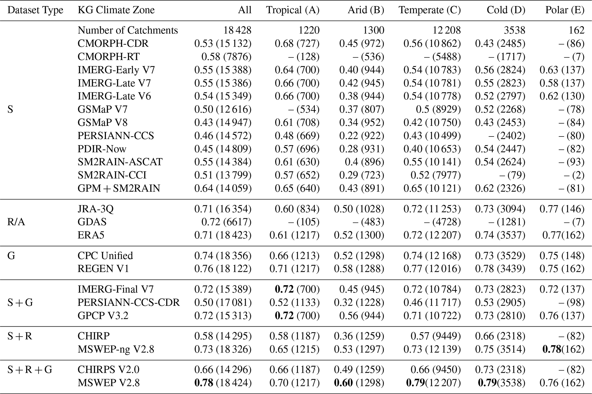
Figure 4 shows spatial correlations between static catchment attributes (Appendix B) and calibration KGE, correlation (r), variability ratio (γ), and long-term bias (β) scores across the catchments. We report these correlations for the multi-source MSWEP V2.8 dataset, the ERA5 reanalysis, and the satellite-based IMERG-Late V7 dataset, to assess how well different catchment attributes predict the performance of each dataset. MSWEP V2.8 and ERA5 exhibit similar patterns, likely because ERA5 is a key input to MSWEP V2.8. For MSWEP V2.8, the strongest predictors of high KGE are low Aridity Index, high P Occurrence, and high Mean NDVI – intercorrelated predictors indicative of humid conditions. For ERA5, the strongest predictors of high KGE are high P Occurrence, low Mean PE, and high Absolute Latitude – conditions that tend to favor frontal P generation. For IMERG-Late V7, KGE is generally less predictable, although high KGE is weakly associated with high Mean P, consistent with tropical regions dominated by convective rainfall. For IMERG-Late V7, a strong predictor of a low β (i.e., P underestimation) is high Topographic Slope, reflecting known difficulties in detecting shallow orographic P and snowfall (Sadeghi et al., 2019; Song et al., 2021). Rain Gauge Density (defined as the number of gauges per 100 km², smoothed using an exponential filter; see Table B1) shows a weak positive relationship with MSWEP V2.8 KGE and r, suggesting that higher gauge density contributes to improved performance, as expected.

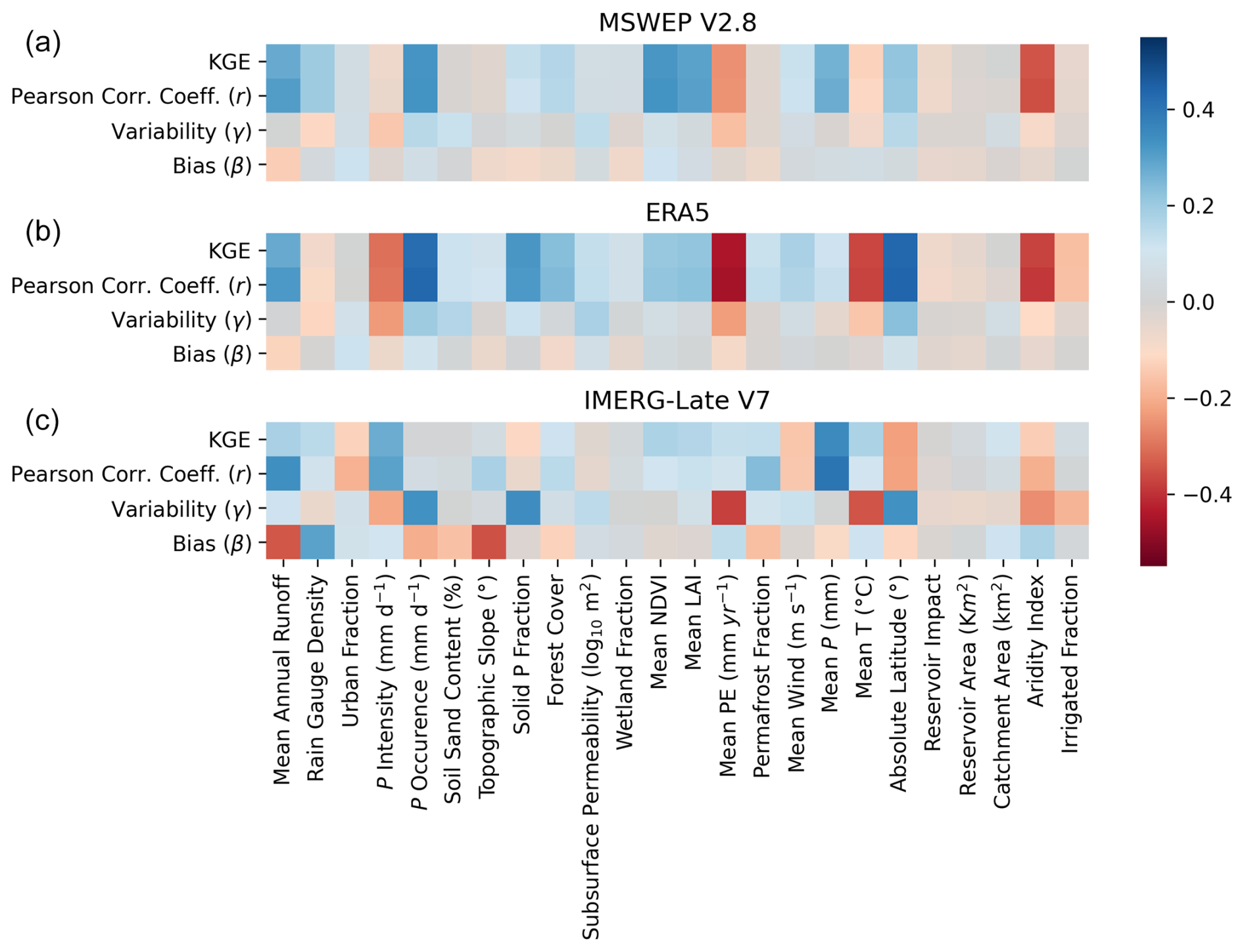
Figure 4 Spatial Spearman rank correlations between static catchment attributes and calibration KGE, correlation (r), long-term bias (β), and variability ratio (γ) scores across catchments for (a) MSWEP V2.8, (b) ERA5, and (c) IMERG-Late V7. See Appendix B for details on the catchment attributes.

To better analyze the influence of catchment-mean topographic slope on calibration KGE for each P dataset, we calculated median KGE values for flat catchments (mean slope <1°) and steep ones (mean slope >7°; Fig. S57a), as well as spatial correlations between KGE and catchment-mean slope values (Fig. S57b). The following conclusions can be drawn:

• Each gauge-based P dataset tends to show better performance in flat catchments than in steep ones (Fig. S57a; e.g., the CHIRPS V2.0 median KGE is 0.05 higher in flat catchments). In contrast, each non-gauge-based dataset performs worse in flat catchments than in steep ones (e.g., the ERA5 median KGE is 0.06 lower). This pattern is further supported by negative spatial correlations between KGE and mean slope for each gauge-based dataset, while the correlations are positive for non-gauge-based datasets (Fig. S57b). The decline in the performance of gauge-based datasets in mountainous regions reflects the sparse gauge coverage in these less accessible, less populated areas (Kidd et al., 2017).

• The tendency for non-gauge-based P datasets to perform better in steep catchments likely arises from the dominance of seasonal, rather than daily, hydrological variability in mountainous regions. These seasonal signals are easier for models to reproduce, resulting in higher KGE values (Beck et al., 2017a). Steep terrain generates high runoff, evaporation is generally low, and streamflow is dominated by slowly releasing snowmelt and groundwater, with limited human modification (Müller Schmied et al., 2014; Beck et al., 2015; Wada et al., 2017).

• Another reason for the stronger performance of (re)analysis datasets in mountainous regions is the ability of NWP models to represent large-scale uplift of moist air over terrain, which produces orographic P (e.g., Pontoppidan et al., 2017; Schumacher et al., 2020). GDAS performs particularly well, likely reflecting the high 13 km resolution of GFS V16.3, which allows more detailed representation of topographic gradients and associated atmospheric processes. JRA-3Q performs least well, consistent with the coarser 40 km resolution of the JMA NWP model as of December 2018 (Kosaka et al., 2024). ERA5 sits between the two, being based on the 31 km IFS model from 2016 (Hersbach et al., 2020).

• The better hydrological performance of each satellite-based P dataset in mountainous regions conflicts with previous evaluations using rain gauges and radar data (e.g., Beck et al., 2019a; Sharma et al., 2020a; Adhikari and Behrangi, 2022). In these studies, poorer performance is generally attributed to surface snow and ice contamination (Cao et al., 2018; Chen et al., 2020), difficulties in detecting snowfall (You et al., 2021; Jääskeläinen et al., 2024; Girotto et al., 2024b), and shallow orographic P (Yamamoto et al., 2017; Adhikari and Behrangi, 2022). Our results suggest that these limitations may be counterbalanced by the simpler, more predictable seasonal streamflow dynamics in mountainous regions.

Figure 5 Median calibration KGE scores for each P dataset across the different streamflow data sources (see Fig. 1a and Appendix A). White indicates that no catchments met the inclusion criteria (Sect. 2.2).

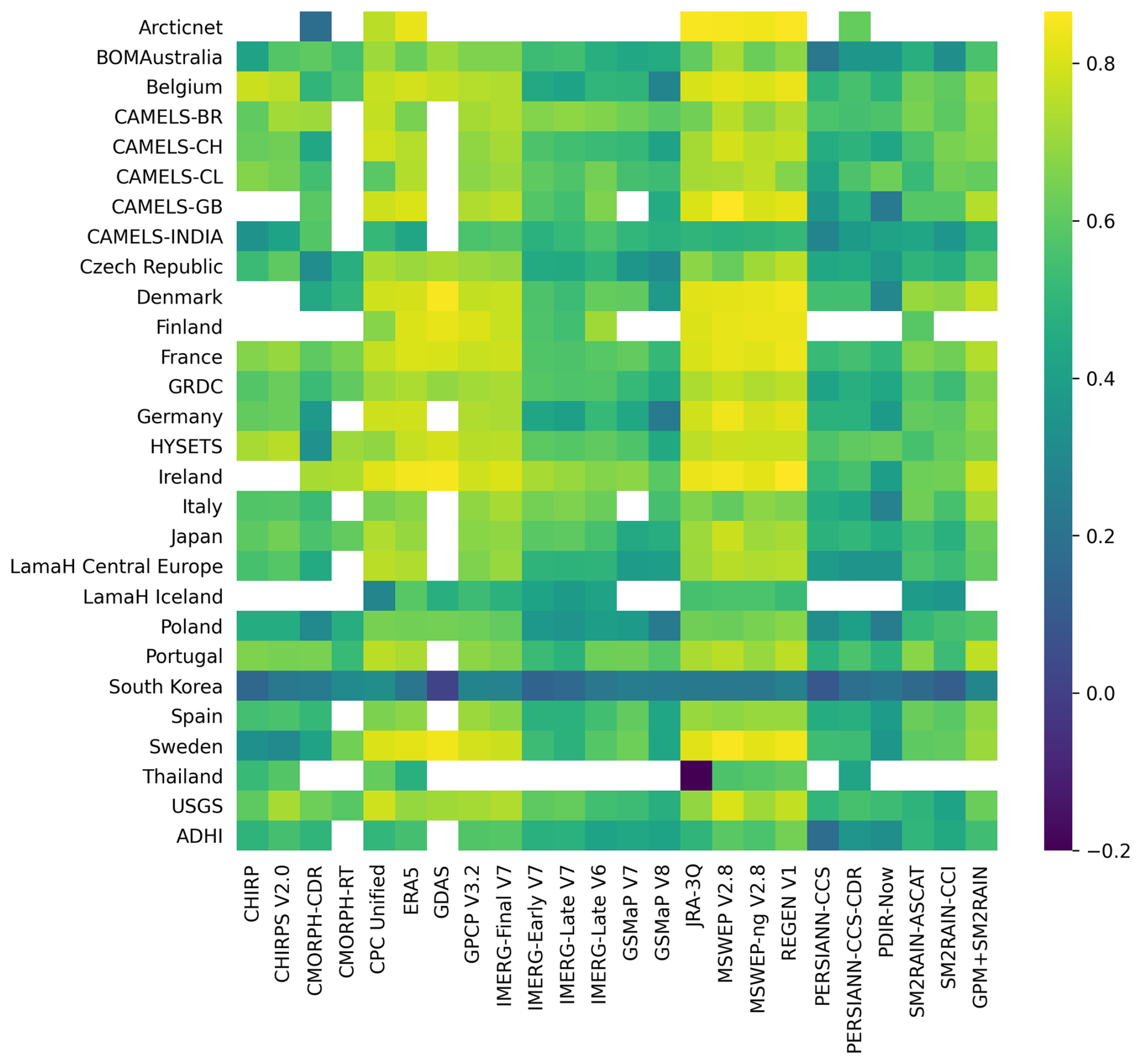
Figure 5 presents median calibration KGE scores obtained from the different P datasets across the various streamflow data sources (see Fig. 1a and Appendix A). Overall performance is somewhat lower for BOMAustralia, CAMELS-INDIA, South Korea, and especially ADHI. Possible reasons for the lower performance for these data sources are discussed below:

• For BOMAustralia (http://www.bom.gov.au/waterdata/, last access: 5 May 2026), the lower performance (Fig. 5) is attributed to arid regions exhibiting consistently low performance (Table 3), with Australian catchments having a particularly high median aridity index of 1.9. Additionally, the presence of numerous small dams used for irrigation, domestic water supply, and flood control likely contributes to reduced performance (Ouyang et al., 2021). Our hydrological model, HBV (Bergström, 1992; Seibert and Vis, 2012), does not explicitly simulate dams, and although we excluded catchments with significant dam influence (see Sect. 2.2), we relied on the GRanD dataset (Lehner et al., 2011), which only includes larger dams. Significant groundwater withdrawals in Australia – also not represented in HBV – may also have contributed to the degraded performance.

• For CAMELS-INDIA (Mangukiya et al., 2025), the main data source for India, the lower performance (Fig. 5) is likely due to extensive human activity, particularly significant groundwater withdrawals (Rodell et al., 2009; Dangar et al., 2021). CAMELS-INDIA catchments have the highest median irrigated area (9.5 %) based on the Global Map of Irrigated Areas (GMIA) V5 (Siebert et al., 2005). Additionally, despite excluding catchments with substantial dam influence, CAMELS-INDIA still has the highest median reservoir influence (defined as total reservoir capacity divided by mean cumulative annual streamflow) across all data sources at 0.04. This suggests that dam regulation may have further degraded performance.

• Similarly, for South Korea (https://water.nier.go.kr, last access: 5 May 2026), the lower performance (Fig. 5) is likely related to extensive human activity, including numerous dams not captured by the GRanD dataset. These dams mainly support domestic and municipal water supply and agriculture (the catchments have a median irrigated area of 6 % based on GMIA).

• For ADHI (Tramblay et al., 2021), the main data source for Africa, arid conditions are likely a primary reason for the low performance (Fig. 5), given a mean aridity index of 1.9 across the catchments (identical to that of the Australian catchments). Another factor is the large number of mostly small dams across the continent that are not included in GRanD. Low streamflow data quality may also contribute, although a global assessment does not fully support this explanation (Crochemore et al., 2020). Additional challenges for rain gauge-based P datasets (CHIRPS 2.0, CPC Unified, REGEN V1, GPCP V3.2, IMERG-Final V7, MSWEP V2.8, and PERSIANN-CCS-CDR) in Africa include sparse rain gauge networks (Kidd et al., 2017), variable data quality, and frequent gaps. For (re)analyses (ERA5, GDAS, and JRA-3Q), limited availability of surface, radiosonde, and aircraft observations for assimilation further reduces performance (https://charts.ecmwf.int/catalogue/packages/monitoring/, last access: 5 May 2026). For ERA5 specifically, spurious P trends in central Africa (see Zsótér et al., 2020) – likely due to changes in the observing system – and intense localized rainfall events (so-called “rain bombs”) in eastern Africa contribute to degraded performance (Hersbach et al., 2020).

• The low median calibration KGE scores for PDIR-Now in Poland, Denmark, and CAMELS-GB (Fig. 5) are associated with median bias (β) values of 1.1, 1.3, and 1.3, respectively (Fig. S27), indicating substantial P overestimation in these regions. Likewise, the low median calibration KGE for JRA-3Q in Thailand (Fig. 5) is mainly due to P overestimation, with a median bias of 4.6 (Fig. S28).

3.3 Potential Limitations and Future Work

We conducted the most extensive evaluation to date of quasi- and fully global gridded P datasets using hydrological modelling. Nevertheless, several limitations should be considered when interpreting the results:

1. The calibration process may potentially suppress certain systematic issues inherent in the P datasets, such as consistent under- or overestimation of peaks, long-term biases, or the presence of drizzle, due to the PCORR and SFCF parameters of HBV. As a result, these issues might not be fully reflected in our calibration scores. However, this should not necessarily be viewed as a limitation. Systematic biases, once identified, are relatively straightforward to correct through post-processing or bias-adjustment techniques. Consequently, penalizing datasets for such deficiencies may be unwarranted.

2. Although HBV has been widely and successfully applied across diverse climates and geographic settings (Seibert and Bergström, 2022), it is a parsimonious conceptual model with a fixed structure and simplified process representations. It does not represent spatio-temporal variability in land cover and land use, or spatial heterogeneity in soils and other catchment properties, and it is driven by catchment-mean meteorological forcings. More complex semi-distributed or fully distributed (gridded) models may yield improved streamflow simulations (Gu et al., 2023); however, we do not expect such models to yield materially different P dataset rankings or alter our main conclusions.

3. HBV does not explicitly represent human influences such as dam operations or groundwater withdrawals, both of which can substantially alter streamflow. Accounting for these processes is challenging because consistent, detailed data on water use and management is generally unavailable. For example, many large dams – and most smaller ones – are missing from global compilations (Zhang and Gu, 2023), and global sectoral water-use estimates are highly uncertain, especially at sub-national scales (e.g., Huang et al., 2018; Puy et al., 2022).

4. We compiled an unparalleled global observed streamflow dataset comprising 35,254 catchments (excluding duplicates) covering all climate zones and latitudes (Fig. 1). Yet, many highly populated and vulnerable regions, particularly in West Asia and parts of Central and Eastern Africa remain underrepresented. This underscores the continued need to improve access to local and regional streamflow data (Krabbenhoft et al., 2022).

5. Since the global distribution of streamflow gauging stations closely aligns with that of meteorological monitoring networks (see Krabbenhoft et al., 2022, and Kidd et al., 2017), our assessment may slightly overestimate the relative performance of gauge-based P datasets and (re)analyses – which assimilate in situ observations from these networks – compared to satellite-only datasets.

6. Some P datasets (GDAS and CMORPH-RT) have relatively short record lengths (Table 1), which can yield less stable KGE scores and may slightly overestimate performance, particularly in arid regions where P events are infrequent. Their limited temporal coverage also prevented the use of a single, uniform calibration period across all datasets. As a result, part of the variation in calibration performance may reflect differences in calibration periods rather than dataset quality. Nevertheless, given the large number of catchments analysed, the impact on the aggregated results and main conclusions is expected to be small.

7. Our assessment was carried out on a daily time scale, which obscures critical sub-daily dynamics, particularly in small catchments and arid regions prone to flash floods. Future research may expand our analysis to sub-daily time scales, which would enable a more rigorous evaluation of the timing and intensity of P estimates. Such a sub-daily assessment would likely improve scores for satellite-based P datasets due to their ability to directly observe events, unlike (re)analyses that rely on approximating when such events occur.

4 Conclusions

The availability of wide range of gridded P datasets, each with unique technical specifications, strengths, and weaknesses, can make choosing the best dataset for a particular application a complex task. To assist users in making better informed decisions, we conducted the most comprehensive assessment to date of (sub-)daily (quasi-)global gridded P datasets using hydrological modeling. We evaluated 24 P datasets across 18,428 catchments worldwide. For each catchment, we calibrated the HBV hydrological model using daily streamflow observations, driven by each P dataset as input. Our main findings can be summarized as follows:

1. Among all P datasets, MSWEP V2.8 consistently achieved the highest overall performance, owing to its inclusion of both satellite and (re)analysis data combined with daily gauge corrections. The best predictors of high KGE for MSWEP V2.8 are low Aridity Index and high P Occurrence. Satellite datasets performed worst overall. GPM + SM2RAIN performed best among the satellite-based datasets, due to its integration of satellite soil moisture and P retrievals. IMERG-Late V7 shows a modest improvement over V6, with gains most evident in arid and cold regions. Among the (re)analyses, GDAS performed marginally better than both ERA5 and JRA-3Q, which exhibited comparable performance. MSWEP V2.8 led among the gauge-corrected datasets, benefiting from its daily gauge corrections, unlike others with 5 d or monthly gauge corrections. Infrared-based satellite datasets showed lower overall scores, with PERSIANN-CCS outperforming PDIR-Now.

2. Regional performance of P datasets varied significantly across climates and data sources, influenced by local P characteristics, topography, data quality, and human activities. Tropical regions favor microwave-based satellite datasets like IMERG due to their ability to capture localized, convective rainfall, while all datasets perform poorly in arid regions, with a slight advantage for (re)analyses. In temperate and cold regions, (re)analyses such as JRA-3Q excel due to their ability to simulate large-scale, frontal P systems. Each gauge-based P dataset shows better performance in flat catchments than in steep ones, whereas each non-gauge-based dataset performs worse in flat catchments than in steep ones. Factors such as aridity, dam presence, and water use likely reduced dataset performance in regions like Australia, India, and Africa. The limited availability of in situ meteorological data, combined with potential streamflow data quality issues, may have further degraded performance in Africa.

3. Despite the comprehensiveness of our assessment, several limitations should be noted. Systematic P biases may have been partially masked during calibration, though these biases can often be easily mitigated through post-processing. Additionally, we employed a relatively simple conceptual hydrological model with catchment-average inputs, although this is unlikely to have affected the results significantly. The overlap in the global distribution of streamflow and meteorological networks may have slightly favored gauge-based datasets and (re)analyses over satellite-based datasets. Lastly, the use of a daily time scale may obscure important sub-daily dynamics, highlighting the need for future sub-daily assessments.

In conclusion, although our findings indicate that datasets like MSWEP V2.8 are well-suited for a broad range of uses, while satellite datasets generally perform worse overall, selecting the most appropriate P dataset ultimately depends on the study region and the specific needs of the application. For example, long-record datasets such as JRA-3Q may be suitable for climate analysis, while IMERG-Early V7 provides a reliable near real-time solution. The continued development of P datasets that balance long-term homogeneity, latency, and spatial-temporal coverage will be essential to meet the varied requirements of users for applications in water resource management, hazard assessment, agriculture, and environmental monitoring.

Appendix A: Streamflow Data Sources

We compiled an unparalleled database with daily streamflow observations and catchment boundaries for 35 254 catchments worldwide, drawing from the 29 data sources listed in Table A1. These sources are divided into two categories. The first category comprises published datasets, including ADHI, HYSETS, CAMELS, LamaHCE, LamaHIce, Germany, and CCAM. For the remaining sources, except GRDC, daily observed streamflow data were obtained from the websites of the respective countries' hydrological or meteorological agencies. Data from GRDC were acquired by submitting an application form on their website and receiving the data via email. For the second set of sources, we used streamflow observations exclusively from stations with available catchment boundaries, allowing us to calculate time series of meteorological forcings for these catchments, including P, temperature, radiation, and humidity. Catchment boundaries for USGS data were sourced from HYSETS, while those for Italy, Spain, France, Poland, Czech Republic, Sweden, Ireland, Denmark, and Finland came from EStreams (do Nascimento et al., 2024). For BOM Australia, Thailand, and Japan, boundaries were obtained from GSHA (Yin et al., 2023). The catchment boundaries for South Korea were acquired from the Environmental Geographic Information Service (EGIS) of South Korea (https://egis.me.go.kr/, last access: 5 May 2026).

Tramblay et al. (2021)Coxon et al. (2020)Mangukiya et al. (2025)Alvarez-Garreton et al. (2018)Chagas et al. (2020)Höge et al. (2023)Hao et al. (2021)Loritz et al. (2024)Arsenault et al. (2020)Klingler et al. (2021)Helgason and Nijssen (2024)

Table A1 Daily observed streamflow data sources, number of catchments, and references/URLs. The number of catchments represents the amount after duplication checks but before suitability checks.

Appendix B: Static Catchment Attributes

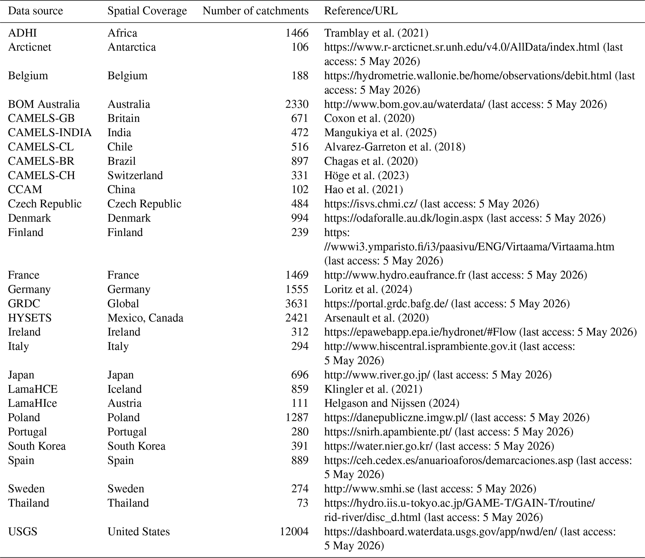
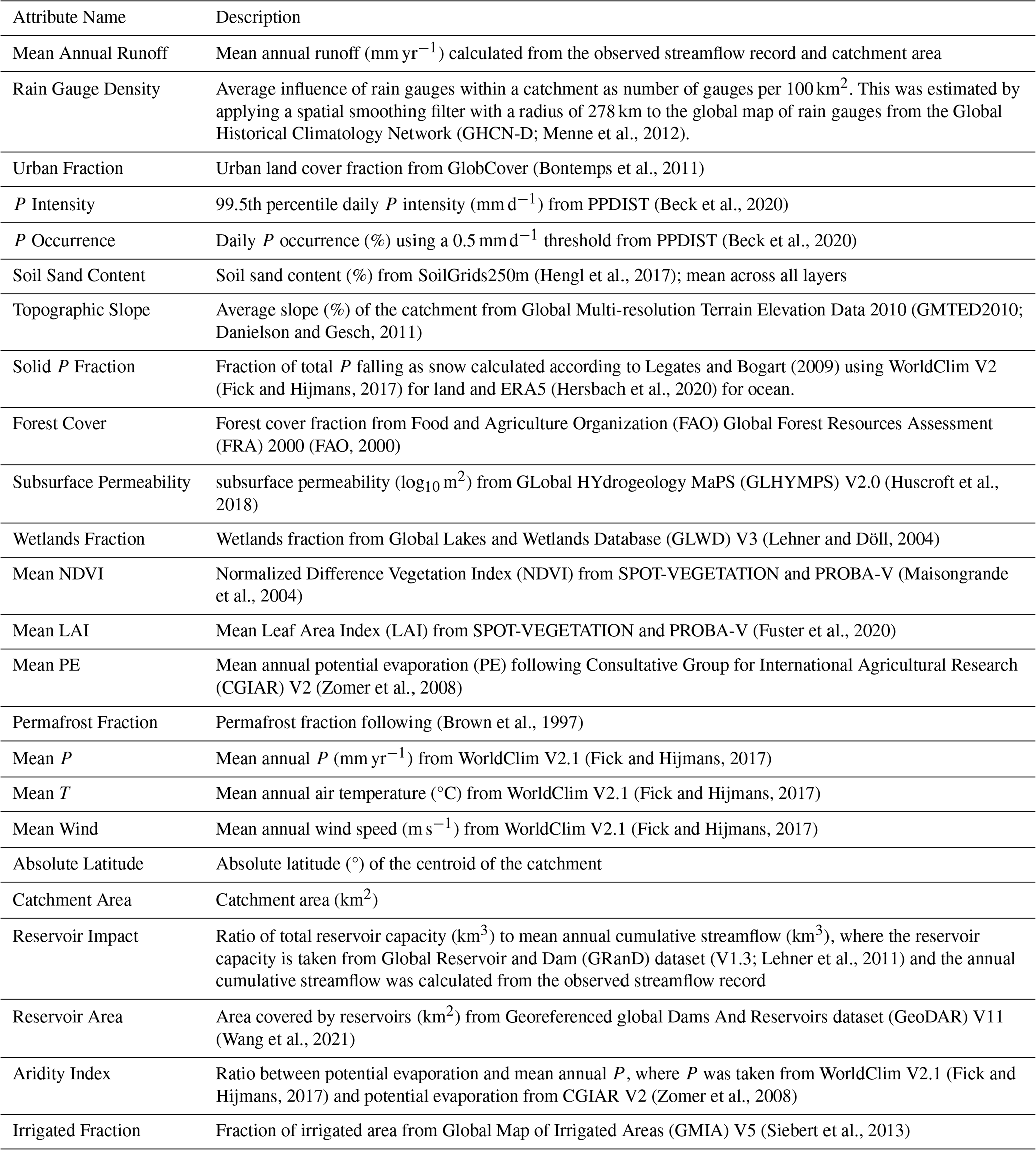
Table B1 presents the static catchment attributes used for assessing performance predictability. Here, “static” refers to attributes that do not vary over time. The attributes were calculated for each catchment as described in the table.

Menne et al., 2012(Bontemps et al., 2011)(Beck et al., 2020)(Beck et al., 2020)(Hengl et al., 2017)Danielson and Gesch, 2011Legates and Bogart (2009)(Fick and Hijmans, 2017)(Hersbach et al., 2020)(FAO, 2000)(Huscroft et al., 2018)(Lehner and Döll, 2004)(Maisongrande et al., 2004)(Fuster et al., 2020)(Zomer et al., 2008)(Brown et al., 1997)(Fick and Hijmans, 2017)(Fick and Hijmans, 2017)(Fick and Hijmans, 2017)Lehner et al., 2011(Wang et al., 2021)(Fick and Hijmans, 2017)(Zomer et al., 2008)(Siebert et al., 2013)

Table B1 Description and sources of static catchment attributes.