the Creative Commons Attribution 4.0 License.
the Creative Commons Attribution 4.0 License.
 | 02 Jun 2026
Long-term hydro-sedimentary dynamics of the Ucayali River (Amazon Basin) revealed through combined observations, remote sensing, and SWAT-Amazon modelling
Alexandre Delort-Ylla
Waldo Lavado-Casimiro
Benoît Camenen
Joana Roussillon
Jhonatan Jr. Pérez Arévalo
Jorge Molina-Carpio
Jean Michel Martinez
The Amazon basin is undergoing increasing environmental changes, potentially approaching a climatic tipping point in the coming decades. Understanding how these changes affect water and sediment fluxes is key for constraining large-scale biogeochemical cycles, yet conventional hydrological networks lack the spatial and temporal resolution required to accurately quantify hydro-sedimentary budgets.
To address this limitation, we develop an integrated, physically constrained framework combining long-term observations, remote sensing, and hydrological–hydraulic modelling (SWAT-Amazon) to quantify multi-decadal hydro-sedimentary budgets and investigate how floodplain inundation controls sediment dynamics in large Amazonian rivers. Focusing on the Ucayali River, a major foreland tributary of the Amazon, this study provides the first detailed, long-term hydro-sedimentary budgets for the Upper Amazon, distinguishing fine sediment fluxes from sand loads.
Results reveal a previously undocumented floodplain-controlled sand sedimentation process: during high waters, large floodplain water storage (up to 19.1 [15.3, 22.9] km3, ∼ 38 % of discharge) reduces main-channel transport capacity, capturing up to 14 % [10 %, 20 %] of the sand flux at peak discharge, while recycling during recession contributes 22 % of the total suspended load at the basin outlet. This dual control partially decouples sediment transport from water discharge. The Andean Ucayali exports 455 [410, 500] × 106 t yr−1 of suspended sediment (40 % sand), of which 36 % is trapped within the floodplain, predominantly as sand (65 % of total deposition). The river delivers 290 [235, 345] × 106 t yr−1 to the Amazon River (26 % sand), making it the dominant sediment source among the Andean foreland tributaries. Uncertainty analysis combining Sobol indices and GLUE simulations shows that, despite substantial equifinality among secondary floodplain parameters, sediment fluxes and associated trapping and recycling fractions remain stable across all behavioural simulations. Budget accuracy is therefore controlled by long-term, multi-variable, multi-source observations rather than by parameter calibration or model structure alone.
These findings demonstrate that floodplains control hydro-sedimentary fluxes in large river systems and act as dynamic regulators of sediment transport, storage, and recycling, with major implications for biogeochemical cycles.
- Article
(10985 KB) - Full-text XML
-
Supplement
(1762 KB) - BibTeX
- EndNote


1.1 Global contribution of the Amazon Basin
The Amazon basin is a massive hotspot for water and matter inputs to the Ocean (Syvitski et al., 2005; Martinez et al., 2009; Moquet et al., 2016; Jouanno et al., 2021; Louchard et al., 2021, 2023) and plays a key role in global hydro-biogeochemical cycles (Gaillardet et al., 1999; Bouchez et al., 2012), capable to significantly impact oceanic biogeochemistry (Jouanno et al., 2021; Louchard et al., 2021). Long-term monitoring by the CZO (Critical Zone Observatory) HyBAm (Hydrology of the Amazon Basin) shows that the Amazon River annually discharges 6500 km3 of freshwater (∼ 20 %–25 % of the global total) (Callède et al., 2010), 1100×106 t of suspended sediments (∼ 8 % of global riverine outputs) (Santini, 2020) and 272×106 t of dissolved matter (Moquet et al., 2016) (∼ 7 % of the global flux). It also influences atmospheric circulation, contributing up to 15 % of global continental evapotranspiration (Salati, 1979; Soares-Filho et al., 2010; Satyamurty et al., 2013) and acts as both a carbon sink and a greenhouse gas source, contributing substantially to global cycles (Richey et al., 2002; Melack et al., 2004; Subramaniam et al., 2008; Ward et al., 2016; Pangala et al., 2017; Louchard et al., 2021). Nutrient-rich from the Andean Cordillera, the Amazon hosts 25 % of terrestrial species and the Earth's largest rainforest (e.g. Lesack, 1993; Malhi et al., 2008; Fan and Miguez-Macho, 2010).
1.2 Role of the floodplain dynamics
Amazonian floodplains act as dynamic reactors, playing a key role in global water and sediment fluxes. Lateral exchanges between the main channel and alluvial plains are of the same order of magnitude as the fluxes reaching the ocean (Meade et al., 1985; Mertes et al., 1996; Dunne et al., 1998) and dominate the annual floodplain water balance (Rudorff et al., 2014a, b). Around 30 % of peak discharge transits through the floodplain (Richey et al., 1989; Lininger and Latrubesse, 2016), with highly variable pathways and residence times (from seconds to months). The flooded area covers 8 %–10 % of the basin (5–6 ×10⁵ km2) (Fleischmann et al., 2022). Thus, flood dynamics regulate the storage and exchange of sediments, nutrients, organic matter, pollutants, and living organisms (Aufdenkampe et al., 2011; Lewin et al., 2017). Sediment residence time varies from brief periods to tens of thousands of years (Mertes et al., 1996; Allen, 2008), depending on the floodplain's geomorphology, influencing chemical maturation processes essential to global biogeochemical cycles, including CO2 consumption by silicate weathering (Guyot et al., 2007; Bouchez et al., 2012). Flexural basins adjacent to the Eastern Cordillera trap 40 %–50 % of Andean sediment exports (Guyot, 1993; Baby and Guyot, 2009; Armijos et al., 2013; Santini et al., 2014; Vauchel et al., 2017; Santini, 2020). Further downstream, sediment balances tend toward equilibrium between deposition and resuspension during flood recession (Santini et al., 2014; Espinoza-Villar et al., 2017), though influenced by the basin's structural Arches. Downstream of the Amazon-Madeira confluence, floodplains have remained only partially filled since the last glacio-eustatic lowstand (∼ 125 m below present sea level) and act as fine-sediment sinks, where large, shallow lakes retain overbank floodwaters (Tricart, 1977; Fleming et al., 1998; Park and Latrubesse, 2017).
1.3 The impacts of global and local changes
The Amazon Basin is undergoing a dramatic transition (Walling, 2006; Malhi et al., 2008; Davidson et al., 2012), facing pressures from deforestation for agriculture and pasture, resources extraction, and construction of hydroelectric projects (Finer and Jenkins, 2012; Latrubesse et al., 2017; Timpe and Kaplan, 2017; Chaudhari and Pokhrel, 2022). In recent decades, the Amazon Basin has also been affected by global climate changes, experiencing more frequent extreme floods (e.g., in 2009, 2012, 2014, 2015) and severe droughts (e.g. in 2005, 2010, 2023, 2024), with an increase in the amplitude of the annual flood wave (Davidson et al., 2012; Espinoza et al., 2012, 2013; Marengo and Espinoza, 2016; Nobre et al., 2016; Towner et al., 2020). Maximum flooding extent along the central Amazon has expanded by 26 % (Fleischmann et al., 2023), mechanically impacting key processes such as CO2 and CH4 outgassing. This warming-induced hydrological cycle strengthening is projected to continue in the coming decades (Hirabayashi et al., 2013; Langerwisch et al., 2013; Sorribas et al., 2016; Alfieri et al., 2017) and the rainforest could reach a tipping point by the second half of the century, potentially converting to savanna, particularly in the eastern and southern regions, or persisting in a degraded state (Lovejoy and Nobre, 2019; McKay et al., 2022; Flores et al., 2024).
1.4 Monitoring challenges and integrated approach
The cascading effects of the ongoing transition in the Amazon remain uncertain, as monitoring is limited, particularly regarding sediment fluxes. Sparse measurements, due to high costs and logistical challenges, hinder the establishment of dense, long-term monitoring networks. Such networks are essential to constrain consistent upstream–downstream mass balances and to spatialize them at relevant scales. This is particularly important for identifying key processes, especially those linked to lateral exchange with the floodplain, which are still only roughly estimated. For instance, the CZO HyBAm covers just one gauging station per 160 000 km2 on average. Additionally, sediment budgets in lowland sub-basins are challenging to estimate accurately, as their order of magnitude is comparable to the uncertainty in sediment load measurements (e.g. Xiaoqing, 2003; Horowitz et al., 2015; Vauchel et al., 2017; Gitto et al., 2017; Santini et al., 2019; Santini, 2020; Dramais, 2020). A significant portion of the suspended load (up to 70 %) consists of very fine sands (Santini et al., 2019; Martinelli, 2022), which are difficult to measure due to their sensitivity to hydrodynamic fluctuations and heterogeneous distribution within the cross section. Furthermore, the buffering effects of such a large basin (Walling, 2006) can mask the impacts on material transfer to the oceans, requiring long-term monitoring.
The scarcity and heterogeneity of observed data directly reduce the robustness and accuracy of hydrological and sediment transport models, limiting their ability to capture key processes and to reliably forecast responses to environmental changes. In response, spatial hydrology has increasingly complemented in situ observations in the Amazon, with satellite data, particularly space altimetry and water color imaging, playing a key role in monitoring water levels and sediment concentrations (Calmant et al., 2009; Martinez et al., 2009, 2015; Espinoza-Villar et al., 2013, 2017; Park and Latrubesse, 2014). On the other hand, hydrological models have also addressed flooding and backwater effects (Yamazaki et al., 2011; Paiva et al., 2013; Pontes et al., 2017; Siqueira et al., 2018; Santini, 2020; Guilhen et al., 2022). Recently, the question of the sediment routing into semi-distributed models has been explored (Fagundes et al., 2021, 2023; Santini, 2020).
However, to date, no study has yet combined remote sensing with modelling to investigate sediment dynamics in detail in the Amazon. Building on long-term CZO HyBAm conventional observations, this study introduces an integrated framework coupling field calibration campaigns, satellite remote sensing, and hydraulic–hydrological modelling to derive process-based hydro-sedimentary budgets for a major foreland tributary of the Upper Amazon: the Ucayali River. Satellite altimetry and satellite-derived fine sediment estimates are used to constrain a hydrological–hydraulic modelling scheme (SWAT-Amazon) simulating water and sand fluxes, with floodplains represented using a simplified reservoir approach.
The objectives are to (i) quantify long-term hydro-sedimentary budgets at sub-basin scale, (ii) investigate the impact of floodplain inundation on water and sediment fluxes, thereby identifying key processes controlling sediment transport, storage, and recycling that remain poorly constrained by conventional river monitoring approaches, and (iii) distinguish the respective contributions of fine sediment fluxes, associated with organic matter and pollutant transfer, and sand loads related to river dynamics.
Unlike previous basin-scale sediment studies in the Amazon, which largely relied on sparse gauging networks or large-scale modelling approaches, this framework provides process-based hydro-sedimentary budgets through multi-source data integration. Given the key role of sediment dynamics in biogeochemical cycles, it also contributes to improving the understanding of the Amazon's role in global material fluxes and of the potential impacts of environmental changes on its hydrology and sediment transport.
1.5 Case study: the Ucayali Basin
Given the continental scale of the Amazon Basin, this study focuses on the Ucayali River, a major foreland tributary draining 350 000 km2 (49 % Andes, 51 % plains). Only two HyBAm gauging stations monitor hydro-sedimentary fluxes in this basin, with incomplete records for the study period (1983–2019): one upstream of the lowlands, the other at the basin outlet. Limited water levels, with some unreliable records, along with a few discharge measurements, are also available from other lowland stations. These constraints make the Ucayali a relevant test site for building the proposed integrated approach, before extending it to other Amazonian sub-basins.
The tailored integrative strategy (Fig. 1) for improving water and sediment balances relies on a combination of three station types in the plain: (i) “low-data” (or poorly monitored) conventional stations, characterized by incomplete and/or inconsistent datasets; (ii) “virtual” stations established at locations where satellite altimetry ground tracks intersect the river mainstem, in order to enhance the spatial density of the monitoring network through the integration of remote sensing and modelling; and (iii) “super” stations with long-term, high-quality datasets, which serve as benchmarks for calibrating and validating the integrated approach. This strategy is further supported by dedicated calibration field campaigns. At all stations, water and sediment fluxes are estimated by integrating remote sensing products and hydrological modelling outputs. Water discharges are simulated using a modified version of the Soil and Water Assessment Tool (SWAT) model (Arnold et al., 1998), to account for Amazon flood wave dynamics and attenuation during flooding. It is assumed that the river transports two particle groups (Santini et al., 2019): fine sediments and sands (Fig. 1b). Fine sediments (mean diameter df≅ 10–20 µm), primarily silts with small clay aggregates, behave similarly to passive scalars and their fluxes are not modelled with transport capacity equations. Instead, fine sediment concentrations at the water surface are derived from satellite images (Espinoza-Villar et al., 2012, 2013, 2017; Martinez et al., 2009, 2015), using an inversion model calibrated with in situ data. Whereas suspended sands (mean diameter ds≅ 80–120 µm) transported in graded suspension, are invisible to satellite spectroradiometers due to Mie scattering (Pinet, 2017). These ranges of mean diameter should be understood as representative values of the dominant PSD modes, rather than strict grain size distribution bounds. Intermediate particle sizes (e.g. coarse silts in the 20–63 µm range) are included within the fine sediment fraction defined by the 63 µm threshold used in the HyBAm monitoring protocol (see Sect. 3.1). Depending on their physical properties, coarse silts may either behave as wash load (e.g. aggregates) or exhibit transport dynamics closer to those of very fine sands when non-cohesive. This supports a first-order bimodal representation of suspended sediment transport at the basin scale, consistent with PSD measurements and vertical grain-size profiles presented in the Supplement (Fig. S1).
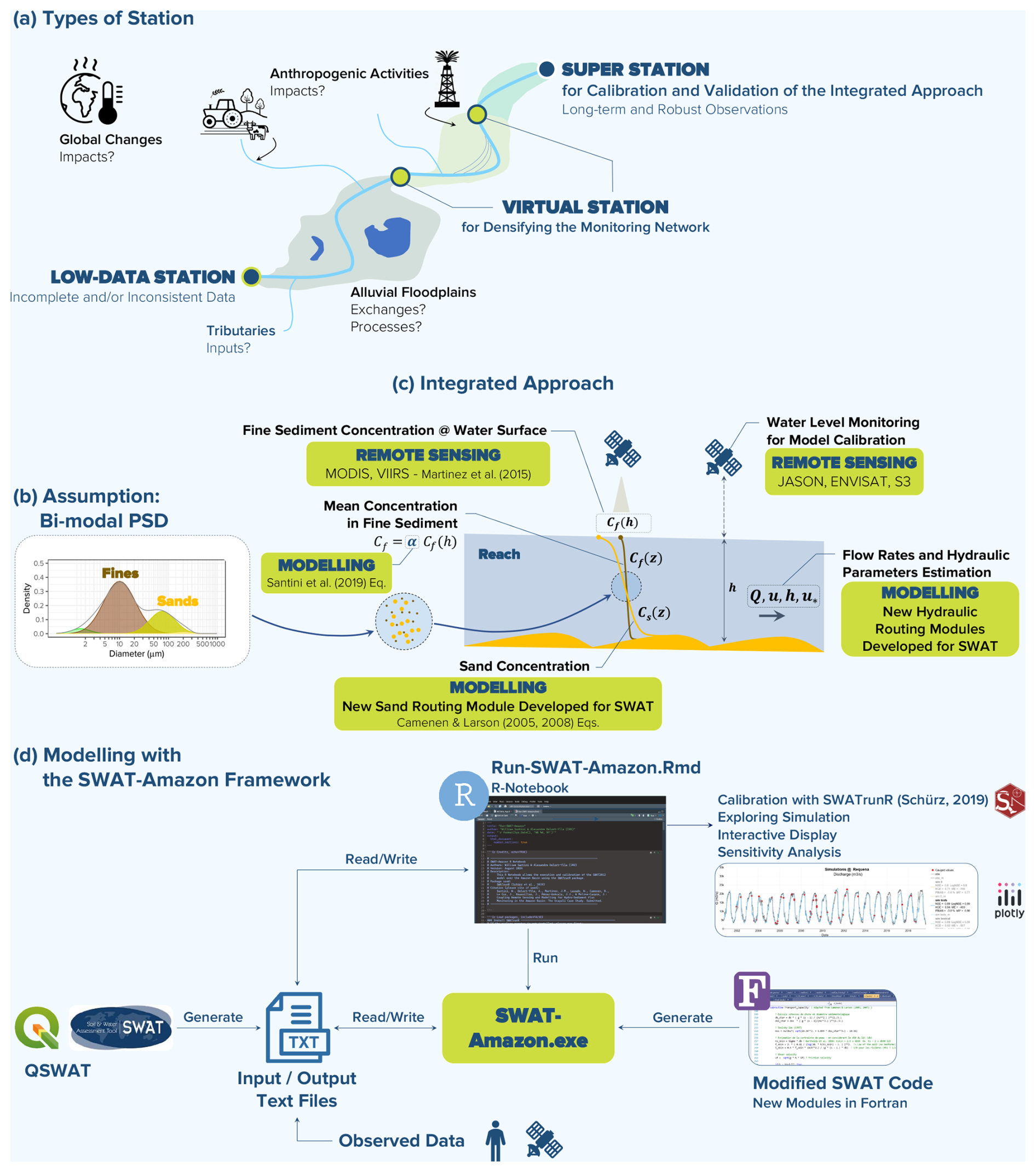
Figure 1General schematic overview of the proposed methodology. Panels (a–c) illustrate the integrative approach. (a) Types of stations. (b) Typical bimodal particle size distribution (PSD) in the large Amazonian rivers, identifying two main size groups: 1 – fine sediments that can be monitored by satellite but not modelled; 2 – fine sands in graded suspension, invisible to satellites but whose transport capacity can be modelled. (c) Integrated approach combining remote sensing, modelling, and calibration campaigns. (d) SWAT-Amazon, a tailored version of the SWAT model for simulating water and sand fluxes. This modelling framework consists of a Fortran-based executable (SWAT-Amazon.exe) and an R notebook (Run-SWAT-Amazon.Rmd) used for model runs, simulation analysis, interactive visualization, sensitivity analysis and calibration with the SWATrunR package (Schürz, 2019).
Moreover, according to Santini et al. (2019) and Martinelli (2022), observed Rouse numbers (Rouse, 1937) are between 0.2 and 0.8 for this sand fraction, inducing concentrations near the surface. Therefore, sand loads are modelled using sediment transport equations in a new routing module developed in the SWAT model, referred to as SWAT-Amazon (Fig. 1d).
3.1 Conventional data
This study relies on long-term hydro-sedimentary flux data from the CZO HyBAm (Guyot et al., 2007; Santini, 2020). In the Ucayali basin, IRD (Institut de Recherche pour le Développement) and SENAMHI (Servicio Nacional de Meteorología e Hidrología) have been operating two HyBAm gauging stations, Lagarto (HyBAm code: 10073500) and Requena (10074800) since 2001 (Fig. 2), carrying out 82 field campaigns to establish rating curves. Additional sediment monitoring was carried out at Puerto Inca between 2012 and 2016, at a conventional SENAMHI station. Water level–discharge relationships were also established at Puerto Inca (10073750) and Pucallpa (10074000), where water levels are monitored by port authorities. Field measurement protocols are described in Sect. S2 in the Supplement. Observed sand fluxes, empirically derived from gauging and surface concentration (S3 in the Supplement), carry ±30 % uncertainties, affecting simulations statistics.
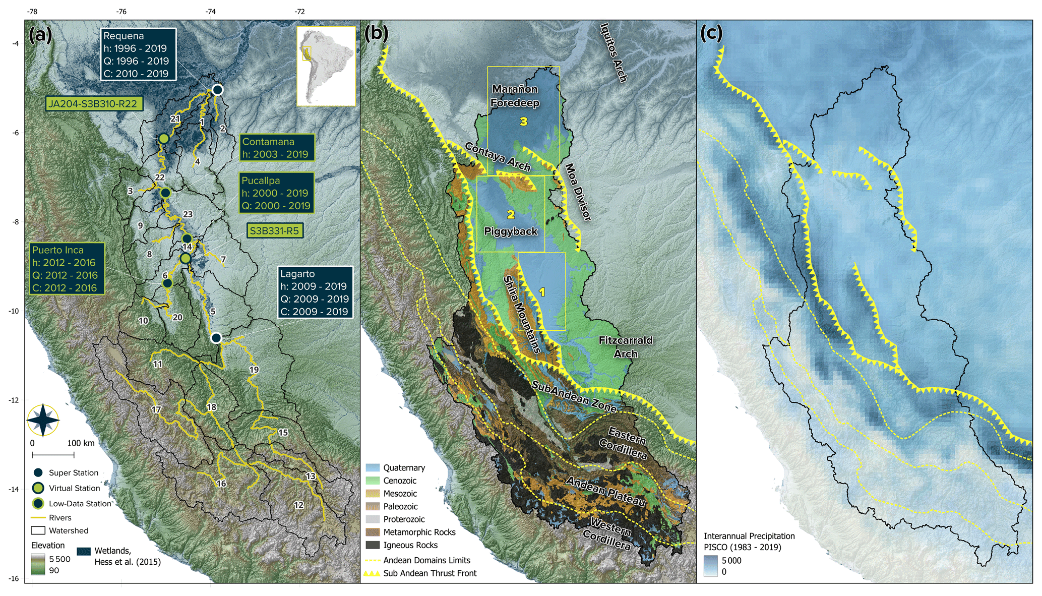
Figure 2Ucayali's stack (a) Ucayali Basin sub-basins and station locations. Super stations (CZO HyBAm) (blue-filled circles, white outline), virtual stations (green-filled circles, blue outline), and low-data Stations with sparse/inconsistent data (blue-filled circles, green outline). The text box details observation periods for water level (h) discharge (Q), and suspended sediment concentration (C). Main Andean tributaries on the left bank: Cushabatay (3); Pisqui (9); Aguaytia (8); Pachitea (10, 20, 6). (b) Geomorphological domains and outcrop distribution. Box 1: Narrow sedimentary basin controlled by Shira Mountains and Fitzcarrald Arch uplift; Box 2: Piggyback Basin backward the Moa Divisor Thrust Fault; Box 3: Marañon Foredeep. Wetlands extent based on Hess et al. (2015). (c) Mean annual precipitation map (PISCO dataset, 1983–2019).
3.2 Altimetric data and definition of virtual stations
Two virtual stations, JA204-S3B310-R22 (reach 22 on Fig. 2) and S3B331-R5 (reach 5), were defined based on the intersection of satellite altimetry ground tracks (Jason, Envisat, Sentinel) with the mainstem of the Ucayali River. These stations provided satellite-derived water level time series used to calibrate the hydrological model. In addition, satellite altimetry was employed to correct water level records at Requena, Pucallpa and Contamana (10074500), the latter being a rarely visited SENAMHI station without any flow measurements. Altimetry data processing was carried out using the open-access VALS (Virtual ALtimetric Stations) software. By summing the virtual stations, the low-data stations (Contamana and Pucallpa), and the long-term CZO HyBAm stations (Lagarto and Requena), the Ucayali sedimentary basin was subdivided into five distinct compartments to establish hydro-sedimentary budgets with the integrated approach.
3.3 Fine sediments monitoring with remote sensing data
3.3.1 Retrieving time series of remote-sensed reflectance data
Given the required revisit frequency and the Ucayali River's width in the plains (500–1000 m), moderate-resolution satellite imagery from MODIS (MODerate Resolution Imaging Spectroradiometer, 250 × 250 m, 1999–present, 1–2 d) and VIIRS (Visible Infrared Imaging Radiometer Suite, 375 × 375 m, 2012–present, 0.5 d) was used to generate time series of surface water reflectance (Fig. 1c). Reflectance values in the red and near-infrared (NIR) bands were extracted pixel by pixel from satellite images using the free software GetMODIS and MOD3R, developed by the CZO HyBAm, that was tested and validated in various previous studies (e.g. Espinoza-Villar et al., 2017; Vauchel et al., 2017). Water masks were applied to the Ucayali River's main course near virtual stations. To ensure 50–100 pixels per mask, large river stems were covered, with masks redrawn every 2–3 years due to river mobility. Collected scenes comprise images spanning 8 d periods, selecting pixels with the lowest cloud cover and smallest satellite-viewing nadir angle.
3.3.2 Conversion of remotely sensed reflectance to fine sediment concentration
Two radiometric campaigns were conducted in the Ucayali Basin: the first in November 2011 at Requena (Espinoza-Villar et al., 2012) and the second in February 2017 at Lagarto, Puerto Inca, and Pucallpa, spanning three weeks (Santini, 2020). A total of 42 surface water samples were collected to determine total, fine, and sand concentrations. Simultaneously, hyperspectral field radiometers (TriOS) were deployed following the experimental setup of Mobley (1999), as adapted by Martinez et al. (2015) for the Amazon Basin. High-frequency (1 Hz) hyperspectral measurements of surface water reflectance were obtained at sampling locations. Relying on this dataset, a unique model for all the Ucayali Basin was fitted between fine sediment concentration at the water surface and the ratio of radiometer reflectance in the NIR (841–876 nm, according to the satellite sensor bands) and red bands (620–670 nm) (see Sect. 5.4). This single relationship is considered applicable along the mainstem of the Ucayali River in the lowland plain because surface reflectance is largely controlled by fine silts of Andean origin, whose grain-size characteristics and optical properties are relatively homogeneous along the river continuum (Martinez et al., 2015; Santini, 2020). In addition, the use of spectral band ratios (NIR RED), commonly applied to reduce the influence of these potential variations in optical conditions (Doxaran et al., 2002; Martinez et al., 2015; Pinet, 2017), supports the applicability of this relationship at the basin scale considered in this study.
3.3.3 From surface to mean concentration of fine sediments
Due to the considerable depth of Amazonian rivers and the vertical sediment concentration gradient near the surface, the ratio αf, relating the channel mean concentration to the surface index concentration retrieved by satellite, ranges from 1 to 1.8 according to the CZO HyBAm database (1.1 to 1.2 in the Ucayali). These values are derived from field measurements of vertical suspended sediment concentration profiles collected at several stations of the HyBAm observatory across the Amazon Basin, including the Ucayali River (e.g. Santini et al., 2019; Santini, 2020). To estimate αf along the river network, the models proposed by Santini et al. (2019) were applied. These models use Rouse-type formulations constrained by observed concentration profiles to describe the vertical distribution of suspended sediments as a function of hydraulic conditions. They were parameterized using hydraulic variables simulated by SWAT-Amazon.
3.4 Input data for modelling
The study utilizes the Peruvian Interpolated Data of SENAMHI's Climatological Observations (PISCO) (Aybar et al., 2020; Llauca et al., 2021) to support the development of an operational model in collaboration with the SENAMHI. Potential Evapotranspiration (PET) was estimated using the Hargreaves and Samani (1985) method, to take advantage of PISCO's temperature data. Land use data was obtained from the Peruvian Ministry of Environment (https://geoservidor.minam.gob.pe, last access: 6 June 2025), while soil information was sourced from the Harmonized World Soil Database (https://fao.org/soils-portal, last access: 6 June 2025). The topography layer was derived from the Multi-Error-Removed Improved-Terrain Digital Elevation Model (MERIT DEM) (Yamazaki et al., 2017), resampled from 90 to 300 m for computational efficiency.
In SWAT-Amazon, water and sand fluxes can be forced at any sub-basin via input files. However, no external forcing was applied in this study. For sand fluxes, we assumed that Andean inflows (basins 3, 8, 9 in Fig. 2) were governed solely by transport capacity within the sand routing module. This assumption is supported by the observed relationship between sand flux and water discharge at Lagarto and Puerto Inca, which indicates, to a first approximation, sediment availability throughout the hydrological cycle in the Andean sub-basins. Lateral contributions from plain tributaries (basins 1, 2, 4, 7) were considered negligible and were likewise represented as transport-capacity limited in the simulations.
SWAT, a semi-distributed model with physical and conceptual equations, was chosen for its proven robustness in simulating hydrological processes in large basins at daily time step. Its open-source Fortran code and extensive user community provide numerous complementary modules and tools. However, SWAT has limitations in modelling water and sediment routing in large rivers with diffusive flood waves and extensive floodplains. It lacks realistic hydraulic connectivity between floodplains and the main channel, preventing accurate simulation of the relationships between water levels, velocities, and discharges, which are keys for sediment transport. To address this, a major code modification is introduced below.
4.1 New water routing modules
The main channel's trapezoidal cross-section in SWAT was replaced with a rectangular one for consistency with the hydraulic equations used. Floodplains were represented using simplified rectangular or triangular cross-sections. Alternative geometries were tested during model development (Santini, 2020), and the selected configuration was retained as the most robust and parsimonious for large low-slope rivers. In this framework, channel geometry parameters represent effective hydraulic conditions averaged at the reach scale rather than the instantaneous geometry of a single cross-section. Although large Amazonian rivers are morphodynamically active and may exhibit lateral migration rates of several tens of meters per year, long-term observations from the HyBAm network indicate that stage-discharge relationships remain remarkably stable over time at the mainstem stations. This suggests that flow conditions are primarily controlled by reach-scale channel geometry over the decadal time scales considered here.
4.1.1 Water level calculation and state variables
The mean water level h (m) is derived from the water volume V (m3) stored in the reach i at time step t (beginning of the simulation day). As long as h≤hf, where hf (m) is the floodplain activation threshold, h is computed as:
where B (m) is the main channel width and Δx (m) is the reach length. When h≥hf, the floodplain is activated, distributing V between the main channel and floodplain. If the floodplain cross-section is rectangular:
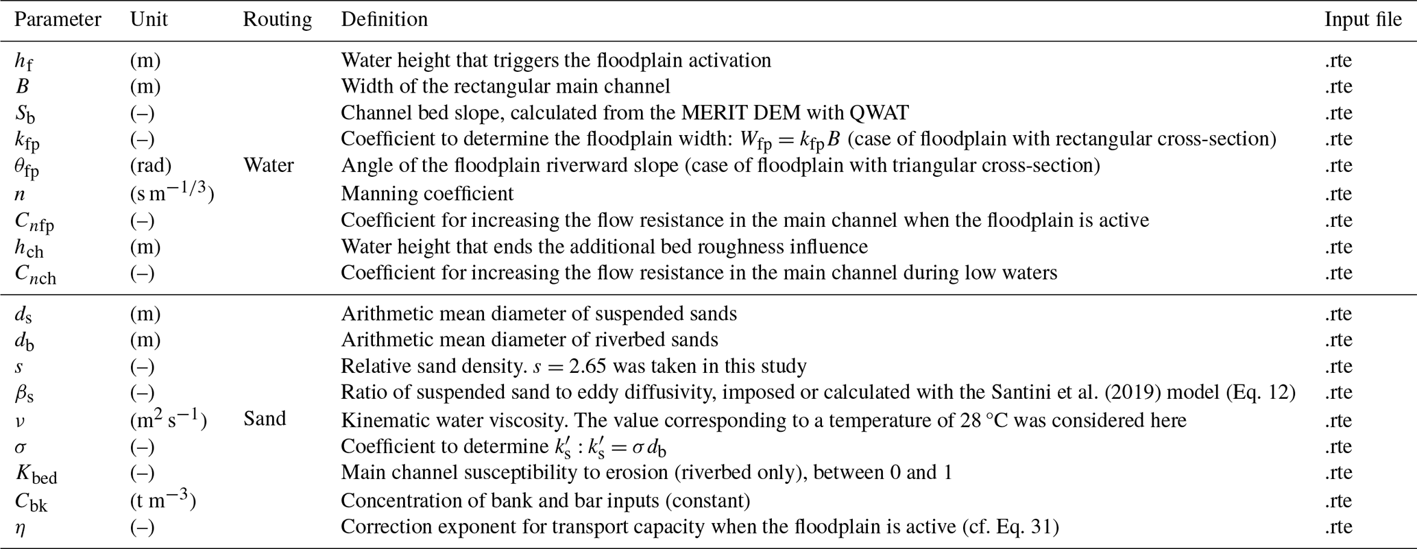
where Wfp=kfpB (m) is the floodplain width and kfp (–) a coefficient to be calibrated (the SWAT-Amazon parameters are given in Table 1). For a triangular floodplain cross-section, h depends on θfp (rad), the riverward slope angle (see S4 in the Supplement). Finally, state variables such as wetted area Ah (m2), wetted perimeter Ph (m), and hydraulic radius Rh (m) are all derived from h.
Table 1Main parameters in the new routing modules of SWAT-Amazon.
4.1.2 Dynamic and process equations
In large Amazonian rivers, flow variations over time and space are minimal, leading to a subcritical hydraulic regime, that can be modelled using the 1D Barré de Saint-Venant equations (Moussa and Bocquillon, 2009). Given the (very) gradual flow variations (Trigg et al., 2009), the convective and local acceleration terms are negligible, making the diffusive flood wave approximation suitable. When water-surface slope effects are also negligible, the pressure gradient is eliminated, allowing the use of the kinematic wave equation. SWAT-Amazon enables reach-specific selection between kinematic wave (Sf=Sb), suitable for steep Andean reaches, and diffusive wave approximation (), preferred for low-slope floodplain reaches where backwater effects may occur (e.g. Yamazaki et al., 2011), with Sf (m m−1) the energy gradient (or friction slope), Sb (m m−1) the bed slope and Sw (m m−1) the water-surface slope. When the diffusive wave model is used, Sw is assessed as follows:
The reach-averaged velocity u (m s−1) and discharge Q (m3 s−1) are then calculated using the Gauckler-Manning-Strickler (GMS) friction equation (Hager, 2005).
In the present study, the diffusive wave formulation was applied throughout the river network in order to account for backwater effects in the low-slope reaches of the Ucayali River.
4.1.3 Continuity equation and water storage in the reach
At the end of the calculation time step (t+Δt), V in reach i is updated as:
where VE (m3) is the volume lost to evaporation, VT (m3) is the volume infiltrated into the unsaturated water table and VR (m3) is the runoff (surface, subsurface, and baseflow) reaching the river. The computation of VE, VT and VR follows the standard SWAT model. The updated volume is then used to determine for the next simulation step.
Although SWAT simulations are reported at a daily time step, river routing is internally solved at a sub-daily time step dynamically determined by the Courant–Friedrichs–Lewy (CFL) stability condition. The routing module automatically adjusts the internal time step to satisfy the CFL criterion and ensure numerical stability (Bates et al., 2010). Daily outputs therefore correspond to the model state at the end of each simulation day.
4.2 New module for sand sediment routing.
4.2.1 Sand load and concentration in the reach
At the beginning of the simulation day, the suspended sand concentration Cs (t m−3) in the reach i is:
where Vs (t) is the sand volume stored in the reach, in the main channel only. The daily suspended sand load Qs (t d−1), taking Δt= 86 400 s, is then:
4.2.2 Transport capacity evaluation
Selecting appropriate transport capacity equations for deep, low-gradient rivers is crucial, as most were derived from laboratory studies under opposite conditions (steep slopes, shallow water, uniform flow). The physically based Camenen and Larson (2005, 2008) models for non-cohesive sands were chosen for their calibration with extensive global datasets and proven applicability in large tropical rivers (Camenen et al., 2014). In these models, the transport capacity (t d−1) for suspended sands is evaluated as a function of the Rouse number Ps (–), which defines the concentration profile exponential shape, and a near-bed reference concentration (m3 m−3), which determines its magnitude:
where s is the relative sand density. The Rouse number summarizes the equilibrium between grain settling velocity ws (m s−1) and turbulence-induced lift, related to the shear velocity u∗ (m s−1), weighted by the sediment-to-eddy diffusivity ratio βs (–):
where κ is the Von Kármán constant. The Soulsby (1997) law is used for estimating the sand grain settling velocity, involving the grain size ds (m) of the suspended sands. The shear velocity is calculated using the depth-slope product:
where g (m s−1) is the gravitational acceleration. The diffusivity ratio is either assigned a fixed value for each reach or computed dynamically using the Santini et al. (2019) model:
The bottom reference concentration is given by Camenen and Larson (2005):
where is the dimensionless grain-related bed shear stress and θcr (–) the critical Shields parameter for the inception of transport (Camenen et al., 2014), which can be estimated from the Yalin-Shields curve as a function of the riverbed dimensionless mean diameter db∗:
The parameter is calculated as following:
where f′ (–) is the Darcy-Weisbach skin roughness factor, derived from the logarithmic velocity law:
with κ is the Von Kármán constant and the height (m) is the hydraulic skin roughness of Nikuradse, which can be expressed as a function of db and a coefficient σ=2.5 (Engelund and Hansen, 1967; Bartholdy et al., 2010):
4.2.3 Sand load adjustment based on transport capacity
The difference (t d−1) between the transport capacity (t d−1) and the sand load Qs (t d−1) is then calculated at time t:
If , there is excess transport capacity, allowing for riverbed erosion. The eroded mass Ebed (t d−1) is defined as:
where Kbed (–) is a coefficient () representing the susceptibility of the channel bed to erosion when the simulated sand transport capacity exceeds the available sand load. This parameter governs the potential entrainment of bed material into suspension and thus the possible contribution of riverbed erosion to the simulated suspended sand flux.
The sand flux is then updated:
Conversely, if , the sand load exceeds transport capacity, and the sand load is set to the transport capacity:
4.2.4 Sand budget at reach scale
Drawing on the mass balance proposed by Dunne et al. (1998), an erosion term, Ebk (t d−1), is introduced to account for both floodplain channel inputs and bank erosion. These processes primarily occur at point bars on the inner bends of meanders, where floodplain inflows, with lower sediment concentrations than the river's transport capacity, enhance erosion and resuspension. Riverbed erosion, Ebed (Eq. 18) and two deposition terms (Dovbk, Dlat), all expressed in (t d−1), are also considered. Riverbed erosion is therefore explicitly represented in the model formulation so that its potential contribution to the suspended sand flux can be evaluated during calibration. Sand deposition on bars in low-velocity zones of the main channel is already accounted for in the sand load adjustment (Eq. 20). Deposition in floodplain channels and levee depressions when active (i.e. when h>hf) is neglected for sand particles, as the high flow resistance caused by vegetation in these areas is expected to result in complete sedimentation at their inlets. This process is therefore implicitly included in the overbank deposition term, Dovbk.
The term Ebk is activated only when the daily water volume ΔVfp (m3 d−1) exchanged between the main channel and the floodplain is negative, meaning floodplain waters contribute to the main channel. Thus, Ebk was defined as function of ΔVfp and Cbk (t m−3), the concentration of these banks and bars inputs, considered as a constant to be calibrated:
Thus, Ebk is neglected when ΔVfp≥0 because the volume of water that could flow back from the floodplain during the rising stages is low compared to the water discharge in the main channel, contrary to the flood recession phase. In addition, the term Ebed can compensate for this if necessary, when the transport capacity is in excess.
The daily sand mass Dovbk is defined as a function of ΔVfp:
where Cs(zsurf) (t m−3) is the sand concentration in the upper flow layer, estimated at (m). Cs(zsurf) is derived from the mean concentration Cs in the reach:
The ratio is estimated with the Santini et al. (2019) model:
4.2.5 Continuity equation
At the end of the calculation time step, the sand volume Vs stored in the main channel of the reach i is updated as:
As for water routing, sand routing is internally solved at a sub-daily time step to satisfy the CFL stability condition. The routed sediment inflow provided by the SWAT-Amazon reach network represents the sediment supply entering each reach and is incorporated into the reach-scale sand mass balance described in Eq. (25).
4.3 Additional flow resistances
4.3.1 Impact of floodplain activation on flow velocity and transport capacity
When the floodplain becomes active, differences in depth and roughness between the main channel and floodplain develop a shear interface between the two flow zones, associated with Kelvin-Helmholtz instabilities, transferring horizontal momentum from the main channel to the floodplain (e.g. Sellin, 1964; Nicollet and Uan, 1979; Ervine and Baird, 1982; Knight, 1989; Knight and Shiono, 1996; Smart, 1992; Loveless et al., 2000; Yen, 2002; Uijttewaal, 2014; Atabay and Knight, 2018; Proust and Nikora, 2020). Sediment-laden water flowing through floodplain channels (Lewin et al., 2017) also transfer large amounts of momentum to the plain and reduces the kinetic energy of the main flow, as does the attenuation of the water surface slope during flooding, which tends toward the valley slope. Moreover, the waters that travel for a short time through the floodplain before returning to the main channel also contribute to reduce the flow velocity. These combined effects significantly reduce flow velocity and, more drastically, transport capacity in the main channel. They change the spatial distribution of velocities and shear stress in the main channel cross-section, especially near the banks and bars, where sediment stocks can be available. To account for this, a flow resistance correction factor ζn was defined as:
where the subscripts “c” and “cf” denote in-bank flow configuration (without floodplain) and flow with an active floodplain, respectively, at the same water level h>hf. To evaluate ζn, the Nicollet and Uan (1979) or Smart (1992) equations can be used. However, both formulations only consider the shear layer interface between the main channel and floodplain. Furthermore, the Smart equation is not suitable for large rivers, and the Nicollet et Uan equation requires an estimate of the floodplain's Manning coefficient. Although the latter was implemented in the new water routing module, a simpler approach was preferred. Therefore, a relationship between ζn and the relative height (–), from which the water exchanges between the main channel and the floodplain begin to affect the flow velocity, was defined:
with Cnfp (–) a coefficient to be calibrated, superior to zero if the flood impacts the flow resistance. Thus, to account for the floodplain drag when h>hf, the Manning coefficient is reevaluated as follows:
In the calibrated model, Cnfp values along the mainstem range between 0.3 and 1. Under typical flood conditions, Y varies between 0 and about 0.3, resulting in an increase of the effective Manning coefficient of approximately 0 %–6 % (see S5 in the Supplement). Larger corrections, up to about 20 %, may occur only during extreme simulated floods when Y approaches 0.5. Such variations are consistent with resistance changes reported in studies of compound channel hydraulics and floodplain–channel momentum exchange (e.g., Nicollet and Uan, 1979; Smart, 1992; Knight and Shiono, 1996; Bousmar and Zech, 1999). The coefficient Cnfp was calibrated during the model calibration phase to reproduce observed stage–discharge relationships at the mainstem gauging stations.
Following the same reasoning as for velocities the ratio of the dimensionless grain-related bed shear stresses and should also be a function of ζn. Indeed, according to Eq. (14):
Here, is assumed, as f′ is a grain-related friction factor, not a flow resistance factor (Yen, 2002): the floodplain drag is already accounted for in ucf, through ncf. The shear velocity term used for calculating the Rouse number (Eq. 10) should be also affected by the floodplain drag:
However, when shifting from a 1D to a 2D framework, the transverse profiles of , and consequently of and , are likely to be more strongly affected than the lateral profile of the depth-averaged velocity (see S6 in the Supplement), in particular near the banks. To account for the complex 2D effects on sediment transport capacity, effects not considered in the initial computation of the transport capacity which was initially calculated using the corrections for and u∗ corrections in Eqs. (29) and (30), the following formulation is applied when the floodplain is active (i.e. when h>hf):
with η an exponent to calibrate which accounts for these complex 2D effects.
4.3.2 Bed roughness influence for low waters
In the large Amazonian rivers, a decrease in bed roughness influence with increasing water levels has been observed (see example in S7 in the Supplement). To model this in the SWAT-Amazon version, the Manning coefficient is modified using the factor ζnch, defined as:
where Cnch (–) is a coefficient and hch (m) the water height below which the additional bed roughness correction activates. Calibrated values of hch range between 35 % and 75 % of the maximum simulated water level across the mainstem reaches, and Cnch between 0.12 and 0.4, resulting in an increase of the effective Manning coefficient of approximately 10 %–30 % at low stage, decreasing progressively as stage rises above hch (Fig. S4). Both parameters were calibrated to reproduce the observed stage–discharge and stage–velocity relationships at the mainstem gauging stations.
4.4 Calibration and sensitivity analysis
The model calibration was performed using the SWATrunR package (Schürz, 2019), which enables parallel processing. To run the SWAT-Amazon executable and calibrate parameters, including the newly introduced ones (Table 1), an R-Notebook was written (Fig. 1d). It allows users to export interactive figures and perform sensitivity analyses. Both SWAT-Amazon and its R-Notebook for calibration are available for download at: https://github.com/william-santini/SWAT-Amazon (last access: 6 June 2025).
5.1 Water discharge simulations
For water discharge, model calibration was performed over the 2010–2015 period based on multiple hydraulic diagnostics (water levels, velocities, and stage–discharge relationships). Model performance was further evaluated using independent hold-out periods and direct comparisons with gauging measurements that bypass rating curves, as detailed in S9 in the Supplement. These complementary evaluations show consistent performance across periods and support the temporal robustness of the model.
At a daily time step, SWAT-Amazon simulations at the watershed outlet show excellent performance (Fig. 3d): NSE (Nash-Sutcliffe Efficiency) = 0.92, KGE (Kling–Gupta efficiency) = 0.95, PBIAS (Percent Bias) = −1.8 %, LogNSE (NSE on the logarithms of the series) = 0.92 over the 2000–2016 observation period used here for inter-station evaluation (see Moriasi et al. (2007) for details on these metrics). SWAT-Amazon significantly improves over the standard SWAT model (NSE = 0.86), using Muskingum routing with maximum flood attenuation. Moreover, the standard SWAT simulation predicts flood peaks 1–2 months earlier than observed, whereas SWAT-Amazon correctly synchronizes them. The model accurately captures hydrological dynamics and interannual variability. As highlighted by Yamazaki et al. (2011), the difference between kinematic and diffusive wave simulations was minimal (not shown), confirming that Ucayali flood attenuation mainly results from floodplain buffering.
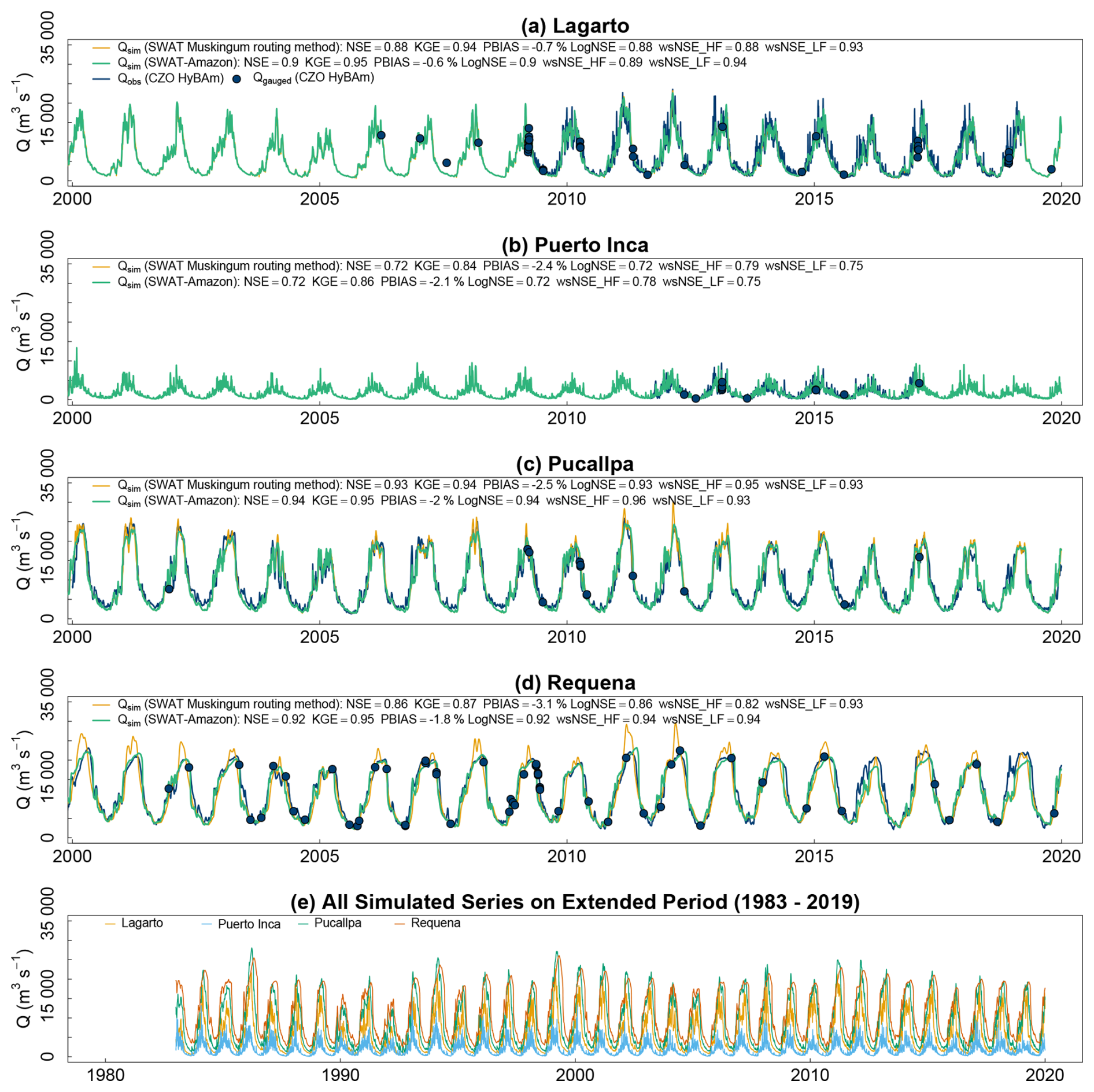
Figure 3Water discharge simulations for the stations with gauging data. (a–d) Observed discharge (marine blue) vs. simulated discharge using the default SWAT model (orange) and SWAT-Amazon (green) at a daily time step, with punctual ADCP gauging values (blue circles). (e) Full 37-year simulation (1983–2019) with SWAT-Amazon for the same station group.
At Pucallpa (Fig. 3c), SWAT-Amazon shows only slight improvements over standard SWAT due to the less developed floodplain. At the Andean outlet (Lagarto and Puerto Inca), where floodplain influence is minimal, both models perform similarly, though SWAT-Amazon slightly outperforms the default version. Despite a good daily NSE (0.72) at Puerto Inca, the model struggles to reproduce rapid flood oscillations typical of piedmont hydrographs. This issue, independent of the routing model, stems from uncertainties in rainfall estimation. Before final calibration, systematic biases (−20 % to +20 %) were observed, with underestimation in piedmont stations and overestimation in plains, primarily due to the precipitation dataset. These biases were corrected using interannual adjustment factors in SWAT .sub files. Additional errors in the PISCO dataset were identified and corrected by standardizing precipitation time series across station subgroups. However, PISCO still underestimated precipitation between Contamana and Requena for 2016, 2017, and 2019, leading to their exclusion from efficiency calculations.
Despite these limitations, the bias-corrected PISCO dataset demonstrated a high degree of homogeneity and robustness, allowing extension of observations across all stations (virtual and conventional) for simulations covering 1983–2019 (Fig. 4e), adding 13 years at Requena and 26 years at Lagarto. This extension is particularly valuable for future studies in this poorly monitored region, especially given the high accuracy of the weighted seasonal Nash-Sutcliffe Efficiency for low (wsNSE_LF) and high (wsNSE_HF) flows (see Zambrano-Bigiarini and Bellin, 2012, for details).
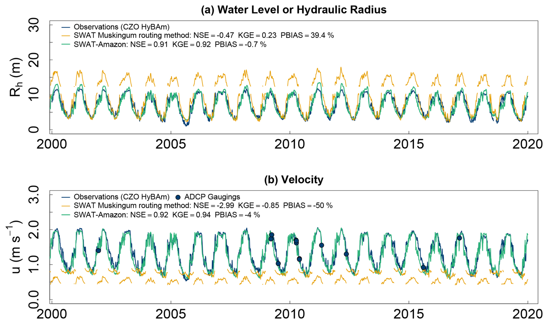
Figure 4Example of (a) water levels and (b) velocities simulation at Pucallpa. Marine blue line: observations, orange line: best default SWAT simulation with Muskingum, green line: SWAT-Amazon simulation, blue filled circle: ADCP gauging values. Error bars, which were less than 3 % for ADCP measurements, are not shown for clarity.
5.2 Water levels, velocities, and rating curves simulations
The hydraulic radius Rh was used to compare simulations with observations (Figs. 4 and 5). Indeed, for large cross-sections, the mean depth hm (m) approximates Rh, and for the modelled rectangular cross-sections, . Moreover, observed water levels were not directly comparable due to offset differences in staff gauge zero-values relative to assumed river bottom elevation. In standard SWAT, once the bankfull height is exceeded, flow instantly spreads into the floodplain, forming a single cross-section instead of the usual approach in hydraulics of separating channel and floodplain flows (e.g. Einstein, 1950; Einstein and Barbarossa, 1952; Yen, 2002). This sudden change in cross-section geometry thus causes a discontinuity in flow velocity and hydraulic radius (Fig. 4), since Ph increases sharply while Ah grows more moderately (). Below bankfull height, standard Muskingum simulations overestimate hydraulic radius and underestimate velocities (Fig. 4), and it is not possible to calibrate u(h) rating curves. Therefore, the standard SWAT model is not able to simulate realistic hydraulic radius (water levels) and velocities and even less sand loads with transport capacity laws, for which these variables are required. Conversely, SWAT-Amazon generates robust daily water level and velocity time series, closely matching observations (Fig. 4), with NSE values between 0.77 and 0.93 for water levels and 0.79 to 0.92 for velocities, the lowest at Puerto Inca, while all others exceed 0.89. It produces consistent Q(Rh) and u(Rh) rating curves (Fig. 5), accurately capturing slope-controlled hysteresis and “duckbill” damping when hf is exceeded, as Manning's coefficient increases with relative water height due to floodplain effects.
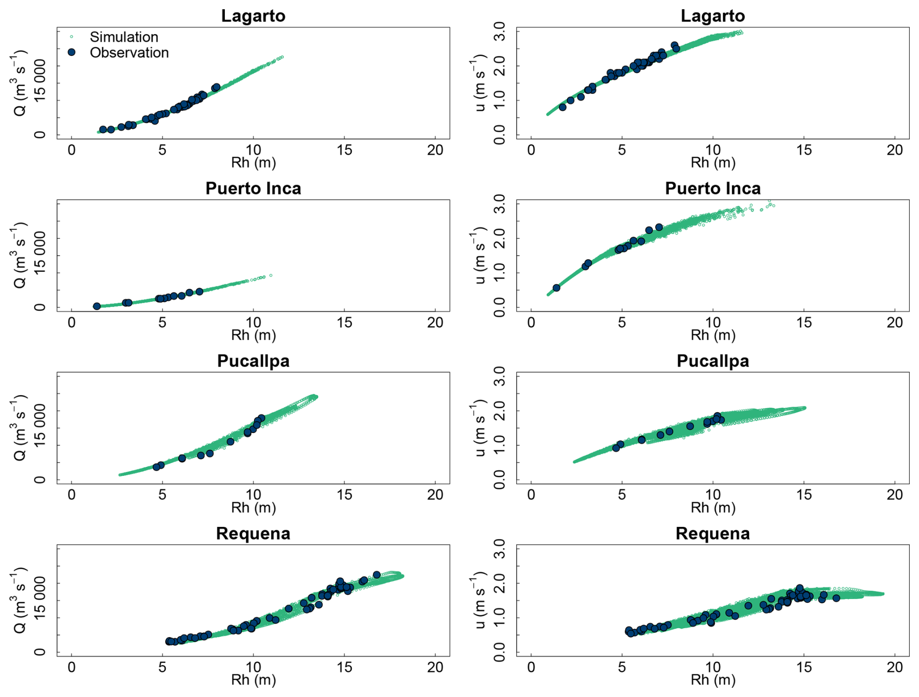
Figure 5Rating curves between hydraulic radius (Rh) and discharge (left) or velocity (right). Green circles: SWAT-Amazon simulation, blue filled circles: ADCP measurements.
5.3 Sand routing
Calibration focused on the September 2009–Augsut 2015 period, when sediment monitoring protocols were enhanced, including higher sampling frequency at Requena between November 2012 and June 2013, where one sample was collected each 2 d plus three sampling repetitions each 10 d. Beyond, sampling was conducted at 5 d intervals during the wet period between July 2013 and September 2015. Additionally, the concentration gaugings were performed in all sites with a higher number of samples collected throughout the cross-section, particularly in the first half of the water column, to ensure more accurate sand concentration calculations. Outside this interval, uncertainties in sand flux observations increase, which complicates the definition of a robust and fully independent validation period (see S9 in the Supplement for a summary of model performance across periods). The lower performance outside the calibration period primarily reflects uncertainties in rainfall forcing and observations, particularly during rapid Andean flood events, rather than a degradation of model performance. To further evaluate model performance, direct comparisons between simulations and gauging measurements were performed (Fig. S6). These complementary evaluations support the temporal robustness of the model despite observational limitations and data heterogeneity.
At Lagarto, the sand routing model accurately reproduces sand fluxes (Fig. 6a, daily NSE = 0.8), validating the capacity-limited flux assumption at the Andean outlet (cf. Sect. 3.4). At Puerto Inca (Fig. 6b, NSE = 0.44), the model struggles due to rainfall data and sharp flux peaks. Nevertheless, at the mainstem level of the Ucayali, the influence of this discrepancy is limited. At Requena, the model closely matches observed sand fluxes (Fig. 6c, NSE = 0.86) with peaks coinciding with maximum rainfall in January-February. From March, sand flux decreases while flow increases, indicating no correlation between sand flux and discharge. This decline is concomitant with the crossing of the threshold hf from which the floodplain watering impacts the transport capacity. In the 2010 drought year, the river briefly reached this threshold, with minimal impact on sand flux: Q and Qss are well correlated. In the remaining years, a second sand peak occurred in May–June. This is concurrent with the recovery of river transport capacity, which is enabled by a reduction in flow resistance due to the dewatering of the floodplain and an increase in energy availability in the main channel, resulting from the influx of floodplain and black water supplies, which have low sediment concentrations. The 2012 extreme flood event, intensively monitored, highlights this key process for sediment routing dynamics.
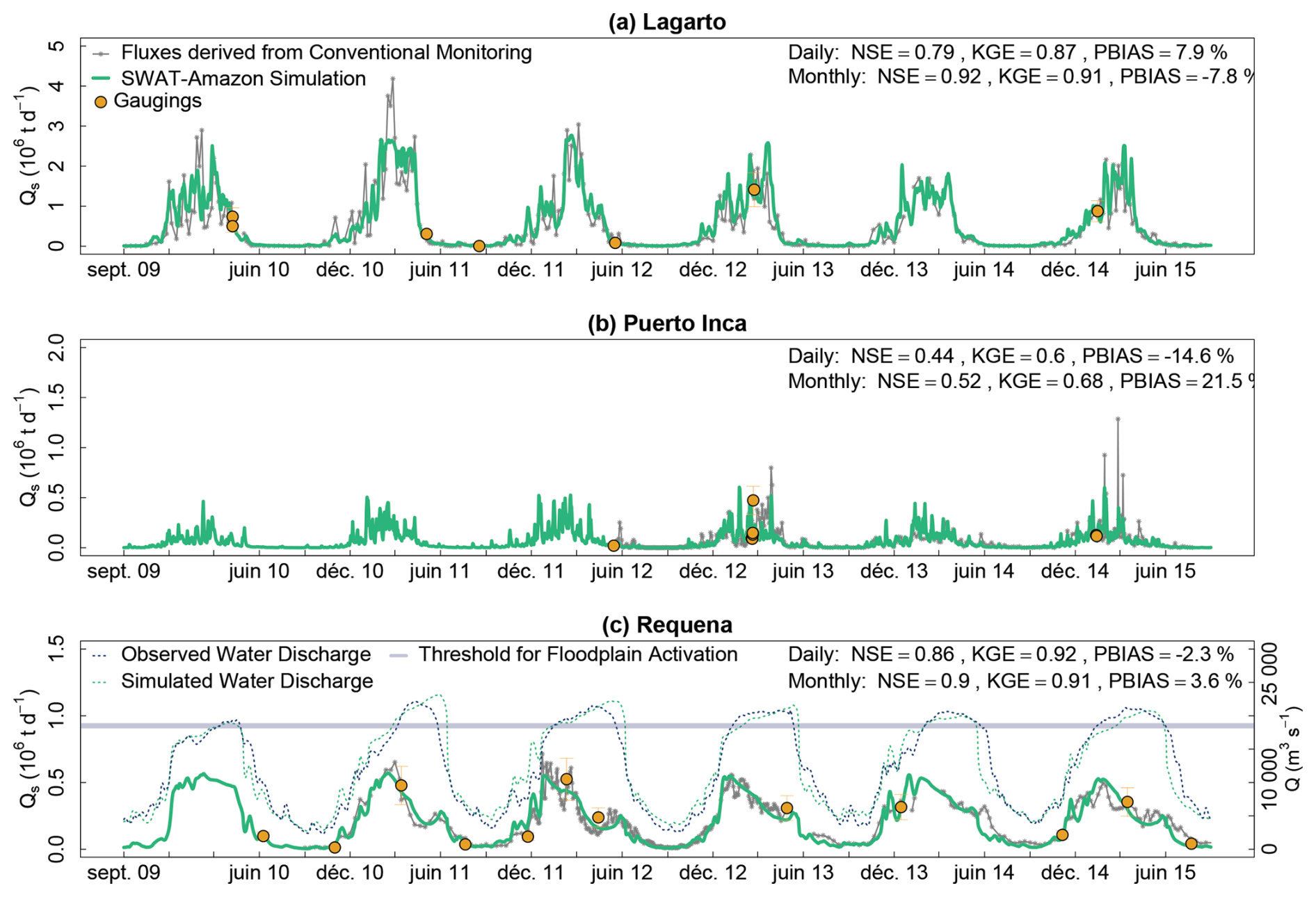
Figure 6Observed and simulated sand fluxes for the gauging stations with sediment monitoring: (a) Lagarto, (b) Puerto Inca, (c) Requena. Gray line with stars: observations, green line: SWAT-Amazon simulations, orange filled circles with error bars: gauged sand flux values. Observed (blue dashed line) and simulated (green dashed line) water discharge at Requena are plotted in (c). The blue horizontal line represents the discharge triggering floodplain activation (corresponding to hf), approximated due to the non-bijective stage-discharge relationship.
5.4 Remote-sensed fine sediments fluxes
Calibration campaigns established a relationship between fine sediment concentration Cf (mg L−1) (at z=h) and the NIR-to-red reflectance ratio R, supporting a single model for the entire basin (Fig. 7) with a high coefficient of determination (R2 = 0.94) and a low Mean Absolute Error (MAE = 59 mg L−1):
This model accounts for reflectance saturation in the red band at high concentrations, providing a better fit across the full concentration range than a simple power-law equation. It was validated across all hydrological conditions from 2000 to 2019 using matchups between time series of in situ fine sediment concentrations monitored at Requena and Lagarto and co-located satellite reflectance ratios at a monthly time step (R2 = 0.78, MAE = 132 mg L−1) (Fig. 7). Note that Eq. (33) is already corrected for adjacency effects, through a simple offset of +0.2 applied to the reflectance ratio to account for water pixel contamination by riverbanks. Finally, the calibration campaigns confirmed that the contribution of suspended sand to the reflectance ratio R is negligible (see S8 in the Supplement).
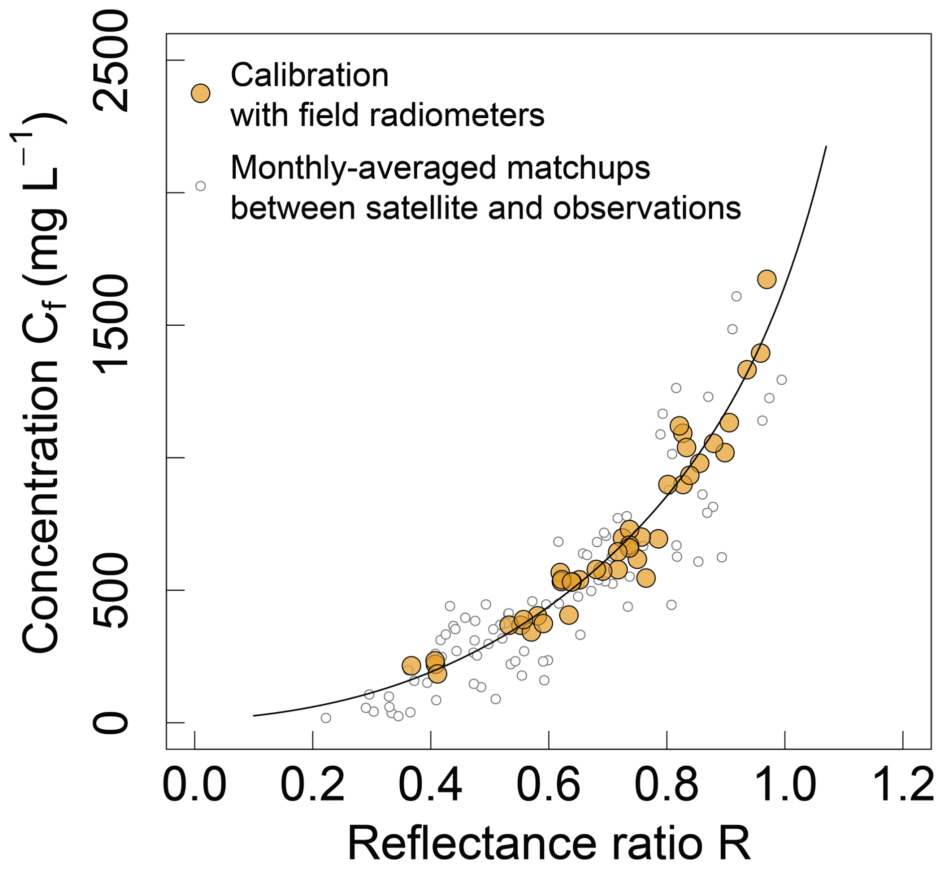
Figure 7Relationship between fine sediment concentration (Cf) at the water surface and the ratio R of NIR to red reflectance. Orange dots represent calibration points, based on 42 field measurements in the Ucayali Basin, where reflectance was measured using a hyperspectral radiometer and fine sediment concentrations were measured at the water surface. Gray dots correspond to matchups between satellite-derived reflectance ratio and fine sediment concentrations monitored at gauging stations, averaged at a monthly time step.
5.5 Validation of the integrated approach at super stations
The integration of remote sensing and hydrological modelling was validated at two super stations in the basin: Requena (Fig. 8) and Lagarto (not shown). Total sediment fluxes (Fig. 8c) were calculated by summing: (i) sand flux (Fig. 8a) from SWAT-Amazon simulations and (ii) fine sediment flux (Fig. 8b) from satellite data combined with SWAT-Amazon flows. The results align well with in situ flux measurements (daily NSE: 0.87 at Requena, 0.79 at Lagarto, monthly NSE: 0.87 at Requena, 0.86 at Lagarto), and suggests that both stations could be monitored in this way with a few calibration campaigns. This supports the definition of minimal observational requirements for transferring the method to other Amazonian basins (see Sect. 6.2.3). The evaluation focuses on variables that directly constrain main-channel hydrology and sediment transport, and thereby indirectly constrain floodplain processes. In the present framework, floodplains are represented using a simplified storage approach, in which water levels are spatially aggregated at the reach scale. However, natural floodplains exhibit strong spatial heterogeneity, including topographic gradients, secondary channels, lakes, and varying degrees of hydraulic connectivity. As a result, local water levels may not directly reflect the large-scale storage dynamics represented in the model. In addition, existing satellite products lack the spatial and temporal resolution required to robustly constrain floodplain water levels and associated storage volumes, particularly given the diversity of water surface types (e.g. secondary channels, connected lakes and isolated water bodies) and their distinct behaviours. Accordingly, local floodplain water levels are not explicitly reproduced; instead, the analysis focuses on constraining water and sediment fluxes and associated storage volumes at the subbasin scale using multi-source observations of main-channel dynamics. The increasing availability of satellite observations over time (Fig. 8b) further strengthens the observational constraints on these fluxes, with missing data mainly occurring at the beginning of the time series due to the progressive deployment of satellite sensors (Terra since 1999, Aqua since 2002, VIIRS since 2012).
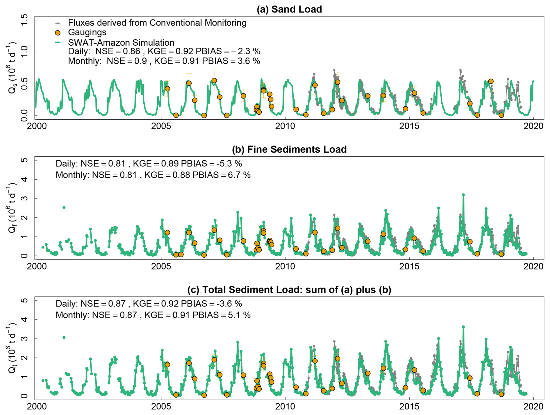
Figure 8Integrated monitoring of sediment fluxes at the basin outlet. The gray line with stars shows observed sediment fluxes, the green line represents SWAT-Amazon simulations, and orange filled circles indicate gauged flux values.
This study presents the first integrated approach for monitoring hydro-sedimentary fluxes in the Amazon basin, providing the most extensive and robust daily time series of hydro-sedimentary fluxes for the Upper Amazon (20 years for fine sediments to 37 years for water discharge and sand flux) with exceptionally high NSE values. It introduces a physically based methodology for modelling transport capacity, using realistic hydraulic parameters derived from the calibration of u(h) and Q(h) rating curves.
Previous large-scale efforts with the MGB (Modelo de Grandes Bacias) model (Fagundes et al., 2021, 2023), contributed significantly to understanding sediment transport across South America. However, challenges remain in representing sand transport, particularly its suspension dynamics. The MGB model assumes that sand transport is predominantly bedload, whereas field observations indicate that sand can account for a substantial fraction of the suspended sediment load in large Amazonian rivers, reaching up to ∼ 70 %. Rouse numbers in the range 0.2–0.8 further indicate transport in graded suspension rather than intermittent transport (Santini et al., 2019; Martinelli, 2022). This conceptual difference likely leads to underestimates of sediment load in the Ucayali Basin in previous MGB applications, with reported estimates being up to nearly three times lower than observations, although its contribution would need to be confirmed through a controlled inter-model comparison. These findings underscore the necessity of detailed, regionally focused studies based on long-term measurements and rigorous data consistency analyses, rather than broad continental-scale assessments, which often involve considerable uncertainties and may lead to misinformed sustainable development strategies and mitigation policies.
For the first time, satellite-based sediment monitoring is applied exclusively to the fine fraction. A relationship (Eq. 33) is proposed that is independent of hydrodynamic fluctuations affecting the surface concentration, since sand contributes from ∼ 5 % to 50 % to the surface concentration in the Ucayali. This contrasts with previous studies (Espinoza-Villar et al., 2012, 2013, 2017; Park and Latrubesse, 2014; Martinez et al., 2015) where satellite reflectance was solely compared with total sediment concentration or where remote-sensing was only used to calibrate the model (Fagundes et al., 2020).
However, Pinet (2017) noted hysteresis in Madeira River relationships due to variations in grain diameter at the water surface, and Santini (2020) suggested that a fraction of fine sediments might also be sensitive to turbulence-induced lift variations. This may introduce limited variability in the relationship during specific hydrological phases, particularly resuspension events and low-water conditions. However, previous studies have shown that such effects are strongly reduced when using the spectral band ratio (NIR RED) (Martinez et al., 2015; Pinet, 2017), with remaining variability comparable to satellite reflectance uncertainty. In addition, evaluation against satellite–in situ matchups across a wide range of hydrological conditions does not reveal any systematic hysteresis at the monthly time scale. As a result, the impact on long-term sediment flux estimates is expected to remain limited relative to other sources of uncertainty and to the overall magnitude of sediment transport.
Before drawing conclusions and interpreting the mass balances (Sect. 6.4), it is crucial to assess the robustness and limitations of the method to ensure that the necessary nuances are applied, particularly at the virtual stations. To this end, a sensitivity analysis of the SWAT-Amazon model was conducted.
6.1 Model sensitivity and equifinality
The Sobol variance-based sensitivity analysis serves a diagnostic purpose: it identifies which parameters require precise measurements for SWAT-Amazon application and which can be assigned wider priors without degrading budget estimates. This hierarchy directly informs the implementation of the Generalized Likelihood Uncertainty Estimation (GLUE) framework (Beven and Binley, 1992), used here for uncertainty propagation (Sect. 6.3.2 and S12 in the Supplement).
The Sobol method was applied to sub-basin 21 over the 2009–2015 period to assess the relative importance of SWAT-Amazon input parameters and their interactions, identifying uncertainties from the model's formalisms. First-order indices (Si) and total-order indices (Ti) were computed to quantify each parameter's individual contribution (with Si) and its total effect (with Ti), including interactions with other parameters, on the overall variance of the model output. The NSE criterion was applied for global outputs (Fig. 9a, d), and the interannual daily average for time-series outputs (Fig. 9c, f). The analysis focused on a selected set of SWAT-Amazon parameters, based on calibration experience and physical understanding, rather than exhaustively testing all parameters. Wide prior ranges were deliberately used to ensure a comprehensive exploration of the parameter space (S10 in the Supplement).
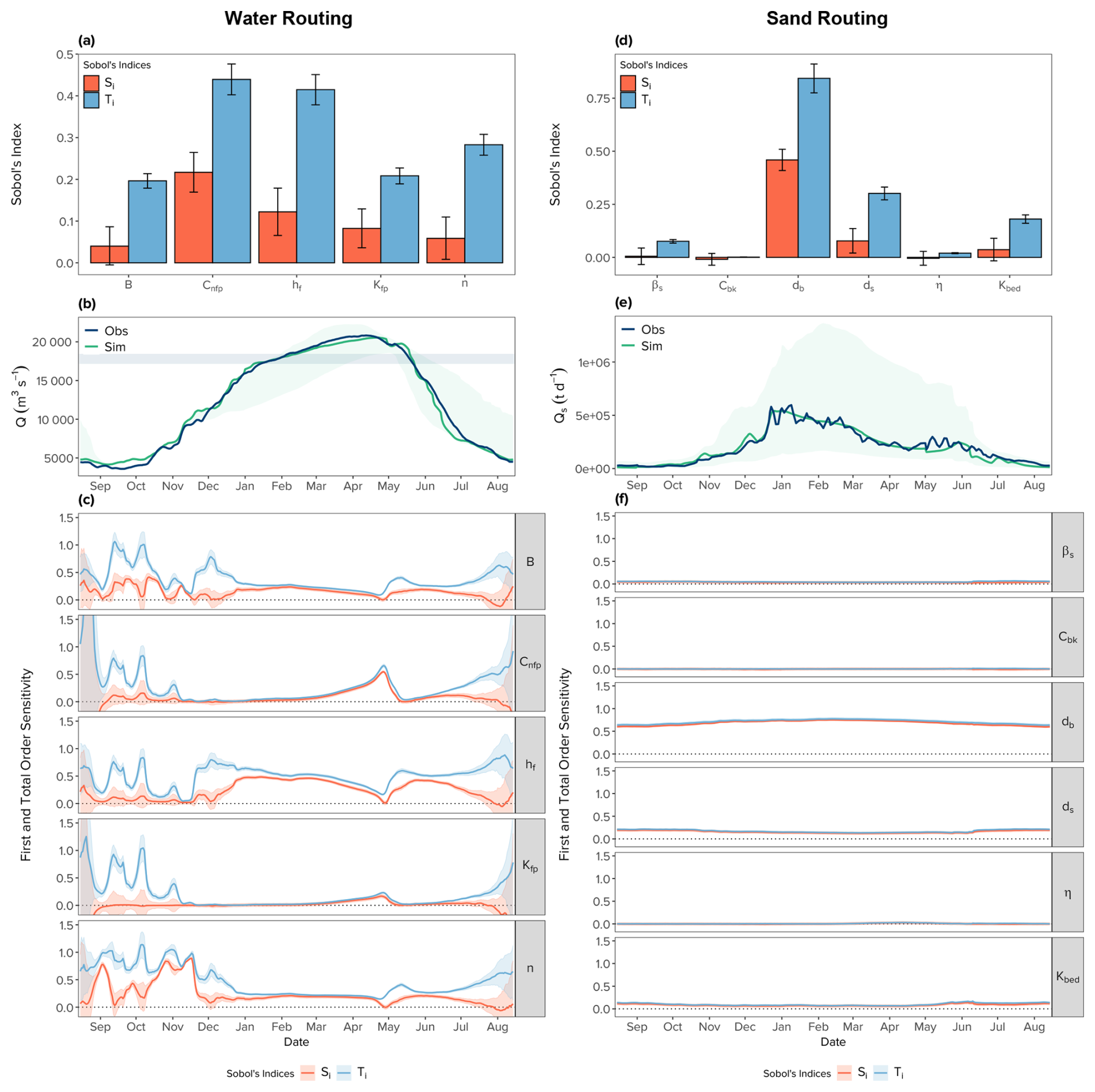
Figure 9Sobol sensitivity analysis results for water (left) and sand routing (right), applied to sub-basin 21 over the 2009–2015 period. (a, d) The analysis based on the NSE criterion, (c, f) summary of the temporal analysis as interannual daily averages. (b, e) The interannual daily average of the observed flux (blue line), the SWAT-Amazon simulation (green line), and the envelope encompassing all simulations performed for the Sobol analysis (light-green ribbon). The blue horizontal line on (b) represents the approximative discharge triggering floodplain activation.
6.1.1 Water routing
The analysis focused on the parameters set (n, B, hf, Cnfp, kfp), with n accounting for all the resistance term . Results show a greater sensitivity of the model to (hf, Cnfp, kfp), which control flood wave attenuation by the floodplain (Fig. 9a). The interannual time-series analysis (Fig. 9c) reveals greater sensitivity during flood recession than rising waters. The recession is particularly challenging to calibrate due to rapid water discharge drops, where even slight shifts in the timing of floodplain recession cause large discrepancies between simulated and observed flows throughout the entire recession limb. Therefore, the parameter hf, controlling recession onset, must be carefully assessed. The strong oscillation of Sobol indices for n during low waters (Fig. 9c) reflects the impact of h (through B) on bed roughness and flow resistance when h<hch (cf. Eq. 32). Small variations of h induce large changes in n during low waters, but with minimal impact on discharge, as shown by the interannual discharge plot in Fig. 9b. This effect diminishes quickly as water levels rise.
6.1.2 Sand routing
The sensitivity analysis, using the parameter set (βs, Cbk, db, ds, η, kbed), shows that db is the most critical calibration parameter (Fig. 9d, f), as previously highlighted by Fagundes et al. (2023). In the present framework, db and ds are assumed to remain constant over the seasonal cycle. Calibrated db values for sub-basins 19, 5, 14, 23, 22, and 21 are 252, 240, 240, 242, 235, and 220 µm, respectively, matching observed mean diameters at Lagarto (260 µm), Pucallpa (243 µm), and Requena (228 µm). Calibrated ds values are approximately 80 µm for all sub-basins, except Lagarto (98 µm), are consistent with PSD observations. Since the calibration of the flood recession limb directly influences sand resuspension (Eq. 22), hf emerges also as a key parameter in sand routing. The influence of kbed is minimal, as the sand load input in sub-basin 21 is sufficient, eliminating the need for riverbed erosion to compensate for sediment supply deficits.
6.1.3 Equifinality analysis
GLUE-based dotty plots were produced by sampling the Sobol-influential parameters over wide ranges (S11 in the Supplement). The water routing parameters (hf, B, kfp, Cnfp, n) all show identifiable optima to varying degrees depending on the reach, consistent with the Sobol analysis. Critically, db exhibits a physical optimum near 220–250 µm matching observed grain sizes, and spurious coarser modes, precluding sand suspension. This bimodality highlights a well-known limitation of purely statistical calibration: without physical constraints, optimization can converge toward parameter values that are mathematically acceptable but physically meaningless. Overall, since db is well constrained and water routing parameters are collectively identifiable, the hydro-sedimentary budgets remain robustly constrained despite residual equifinality across all behavioural simulations (S12 in the Supplement). These findings justify the use of expert measurement-informed priors for uncertainty propagation.
6.2 Calibration insights from the SWAT-Amazon method
In the hydraulic routing method (Sect. 4.1), compensating hydraulic effects limit the influence of B and n on routed discharge. Reducing n increases flow velocity u and discharge Q (Eq. 5), which decreases the water volume stored in the reach and therefore h (Eq. 1). The resulting decrease in cross-sectional area leads to a proportional reduction in u and Q.
Therefore, when h<hf, discharge calibration relies exclusively on the default SWAT rainfall-runoff model. However, u and h are directly related to the parametrization of n and B and are the primary variables in the transport capacity model utilized here (Sect. 4.2). Q is also a key variable (Eq. 9). As B is poorly-known, it was excluded from Eqs. (6) and (8) of the transport capacity model by replacing B h with and u B with . With regard to n, another significant source of uncertainty, it should be noted that this variable is not included in the transport capacity equations. This is because u is used and calibrated prior to the Qs computation.
6.2.1 Calibration strategy for a super station
According to the previous analyses, the calibration strategy for stations with robust, long-term hydro-sedimentary monitoring is:
- a.
Start by calibrating Q in each reach, for hf only, using the SWAT's default hydrologic parameters.
- b.
Calibrate Q, considering floodplain effects, using hf, Cnfp and kfp (or θfp).
- c.
Calibrate u and h by adjusting n and B only; Q is unaffected by this calibration.
- d.
Check the relationships Q(h) and u(h), revisiting step c if needed.
- e.
Compute the , independently of n and B. If necessary, adjust Qs using parameters in Table 1, particularly db, the most sensitive parameter.
It is important to emphasize that the optimal calibration for water discharge may not align with the best calibration for water level, velocity, and sand load time series. A compromise must be made.
6.2.2 Calibrating virtual and low-data stations with satellite altimetry
The sensitivity of the model to n and B emphasizes the importance of h (Eqs. 1, 2, 4) in the routing module, particularly for floodplain inundation and dewatering triggers (Sect. 4.1), as already discussed above. For ungauged reaches (5, 23, 22, see Fig. 2a) in the plain, n and B can be calibrated using relative water levels (hydraulic radius) derived from spatial altimetry and shifted by a constant offset to match simulations (Fig. 10). The Manning coefficient is supposed already known to a reasonable degree, as coherent values of ± 0.0005 s m have been found across all the other plain's sub-basins. Given the large sub-basins and significant channel lengths, bed slope errors are assumed to be smoothed, and therefore Sb also well assessed. Thus, velocities can be reliably determined if B is calibrated through h calibration. The calibration for reaches (5, 23, 22) was also guided by looking for the best simulation at Pucallpa and Requena.
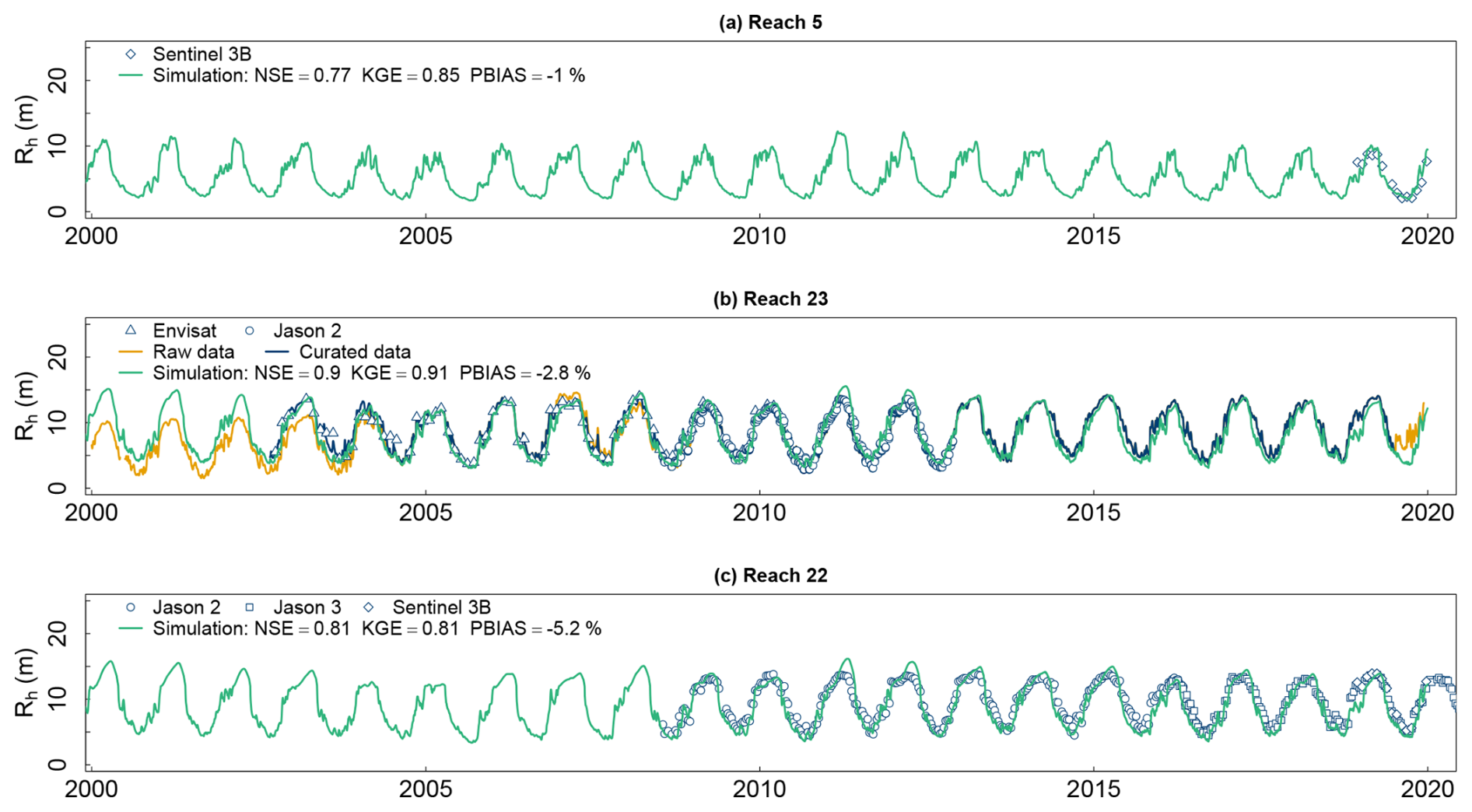
Figure 10Calibration of ungauged reaches using satellite altimetry: Satellite-derived water levels (blue points) shifted by a constant offset to match simulations: triangles (Envisat), circles (Jason-2), squares (Jason-3), diamonds (Sentinel-3B). Conventional in situ observations appear as an orange line, while the curated series incorporating satellite altimetry is in blue. SWAT-Amazon simulations are shown in green. (a) Reach 5 (virtual station S3B331-R5), (b) Reach 23 (Contamana), (c) Reach 22 (virtual station JA204-S3B310-R22).
Finally, implementing an integrated approach combining modelling and remote sensing for monitoring hydro-sedimentary fluxes would require revisiting hydrological network operations. Specifically, a few gauging campaigns (around four, strategically timed along the annual hydrograph) could be sufficient for model calibration. Additionally, synchronizing gauging with satellite altimetry would enable the construction and simulation of robust rating curves.
6.2.3 Minimum observational requirements
Based on the long-term monitoring experience of the CZO HyBAm network and the results obtained in this study, the framework can be applied to other Amazonian basins provided that a minimal observational dataset is available at a limited number of super stations and complementary virtual stations. For the last ones, this includes: (i) approximately four to eight discharge gauging campaigns covering the main stages of the annual hydrograph (rising limb, high water, falling limb, and low water), (ii) a comparable number of suspended sediment gaugings distributed along the hydrograph and carried out using standardized and hydraulic-based protocols (Santini et al., 2019), (iii) one to two detailed PSD surveys in relatively homogeneous upstream reaches, increasing to four to five in more heterogeneous downstream settings (e.g. below major confluences), and (iv) two to three radiometric calibration campaigns spanning contrasted hydrological conditions.
6.3 Framework limitations and uncertainty
6.3.1 Model structural limitations
This study adopts a hydraulic representation of the river, modelling the floodplain as a reservoir. Rapid exchanges through secondary channels are neglected, and their influence is approximated on discharge propagation through a minor adjustment of the Manning's coefficient. Guilhen et al. (2022) used a previous version of SWAT-Amazon with a slightly modified floodplain configuration, allowing 1d floodplain flow through its whole cross-section with a Manning-Strickler equation. However, in addition to being almost impossible to calibrate, the floodplain flow being extremely sensitive to the floodplain Manning coefficient because of its huge cross-section, the changes in terms of results were extremely negligible: less than 1 % of the water discharge in the main channel, well below expected model precision.
Another key assumption in SWAT-Amazon is the absence of backflow from the floodplain to the main channel during the rising limb. Observations in the Amazon basin support this, as low-gradient floodplain channels often experience tributary flow blockage, with the Tapajós River in Brazil being an extreme example. However, during deflooding, floodplain drainage dynamics differ from flooding processes. In SWAT-Amazon, these dynamics are governed by floodplain cross-section geometry. Introducing a Maillet-type law could improve recession representation, but discrepancies in timing appear mainly driven by rainfall variability, masking this effect. Thus, no modifications were made.
Floodplain sediment concentration during deflooding was assumed constant. Nevertheless, the unique monitoring of sediment concentration in a floodplain channel, performed at Lago Grande de Curuai (Brazilian Amazon) shows a decrease from ∼ 800 mg L−1 during low-waters when the floodplain water flows back into the main channel to ∼ 40 mg L−1 when the channel is under the influence of the Amazon River, with a mean concentration of 135 mg L−1 (Moreira-Turcq et al., 2013). This value appears to be relatively close to that calibrated for Cbk (for the sand fraction only) at sub-basins 23, 22, and 21 (∼ 180 mg L−1).
A dynamic law linking Cbk to water level could refine peak resuspension modelling but requires concentration data for calibration. Alternatively, Fagundes et al. (2023) treated the floodplain as a homogeneous sediment reservoir, balancing suspended fluxes with settling. However, this method applies only to clay and silt, excluding sand, and the settling law can be challenging to calibrate in the absence of observational data. Given floodplain water storage timescales (months), most fine sediments likely settle before being remobilized. Furthermore, as underscored in the introduction, sediments resuspended during recession can be centuries to millennia old, indicating long-term floodplain recycling rather than short-term remobilization.
Lastly, the distinction between Ebk and Ebed is partly supported by the calibration experiments. When bed erosion is activated (kbed>0), the model tends to generate rapid and abrupt peaks in simulated sand flux once the transport capacity exceeds the available sand load, whereas adjusting Cbk produces a smoother and more progressive increase in sand concentration that better reproduces the secondary peaks observed during the recession phase. The calibrated values of Kbed remain very small (Kbed≪1), suggesting that riverbed erosion contributes only weakly to the simulated suspended sand flux in the main stem, although a minor contribution cannot be fully excluded.
6.3.2 Framework uncertainty
A GLUE-based uncertainty analysis was conducted over a Latin Hypercube ensemble of 2500 simulations (S12 in the Supplement), scoped to routing and sand transport parameters, conditional on the hydrological forcing, with physically informed priors (Sect. 6.1).
For discharge and sand flux, GLUE-weighted envelopes (5th–95th percentiles) remain narrow relative to the interannual amplitude, indicating that parameter uncertainty propagates weakly compared to the magnitude of hydrological variability and that the dominant dynamics are robustly constrained. Envelope width depends jointly on data availability and measurement quality, which act as coupled controls on parameter identifiability rather than independent sources of uncertainty. Floodplain water storage uncertainty in particular is strongly controlled by hf, emphasizing the need for accurate stage–discharge rating curves to constrain this parameter reliably (Sect. 6.2.3). Importantly, because the budget indicators (trapping and recycling fractions) depend primarily on hf, B, and db, which are well-constrained parameters (Sect. 6.1.3), they remain robust across the behavioural ensemble despite the wider prior ranges assigned to less identifiable floodplain parameters. This structural stability is confirmed by the GLUE-propagated budget envelopes (S11 and S12 in the Supplement).
Fine sediment fluxes achieve low bias and good performance metrics (Fig. 8b), yet exhibit wider uncertainty envelopes. This apparent performance is largely driven by the dominant seasonal signal rather than true predictive skill. Satellite retrieval errors cancel over long-term integration, masking short-term variability: the method reliably captures the mean seasonal cycle, but not its anomalies. Satellite radiometry is therefore robust at the climatological scale but not at the event scale.
Both conclusions rest on a common foundation: physically meaningful uncertainty quantification requires prior knowledge, which itself requires long-term, multi-variable observations, as provided by networks such as the CZO HyBAm. Uncertainty is therefore not only a modelling issue, but fundamentally a data-structure constraint. Model calibration and interpretation depend on sustained fieldwork and on a detailed understanding of measurement protocols and data limitations. As a result, rigorous data governance, FAIR practices, and strong research–operational links are essential for reproducibility and long-term continuity.
6.4 Hydro-sedimentary dynamics in Amazonian foreland systems: long-term insights
The robustness of the results enables precise water and sediment balances, distinguishing fine particles from sand, at each virtual and conventional station (Fig. 11). This is achieved at an unprecedented spatiotemporal resolution over the periods 1983–2019 (37 years) for water and sand fluxes and 2000–2019 (20 years) for fine sediments.
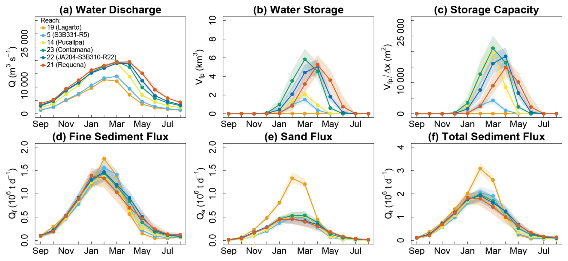
Figure 11Interannual water (1983–2019) and sediment (2000–2019) balances along the Ucayali River. Lines show interannual monthly means and shaded bands represent the 5th–95th percentile envelope of the behavioural GLUE ensemble (2500 runs). (a) Water Discharge. (b) Floodplain water storage (Vfp) in km3. (c) Normalization of Vfp by the reach's length (Δx) for cross-sub-basin comparison. (d) Fines suspended sediments. (e) Suspended sand fraction. (f) Total suspended sediment load. See S12 in the Supplement for full uncertainty propagation details.
6.4.1 Dynamics of flood waves, flooding, and sediment transport
Water and sediment peak fluxes at the Andean outlet occur in February (Fig. 11), declining sharply from March to May as Andean precipitation decreases. The sediment flux at the basin outlet is strongly correlated with Andean discharge (Fig. 12c), confirming the Andes as the primary sediment source. This results from intense erosion along the Eastern Cordillera and Sub-Andean thrust belt, where high precipitation erodes Paleozoic and Mesozoic sedimentary sequences incorporated into Cenozoic deposits eastward as the orogenic prism advances through crustal shortening and thickening (McQuarrie, 2002a, b; Espurt et al., 2008; Gautheron et al., 2013; Pfiffner and Gonzalez, 2013). Additionally, the Central Andes' convex hypsometric profile (Montgomery et al., 2001) promotes deep fluvial incision.
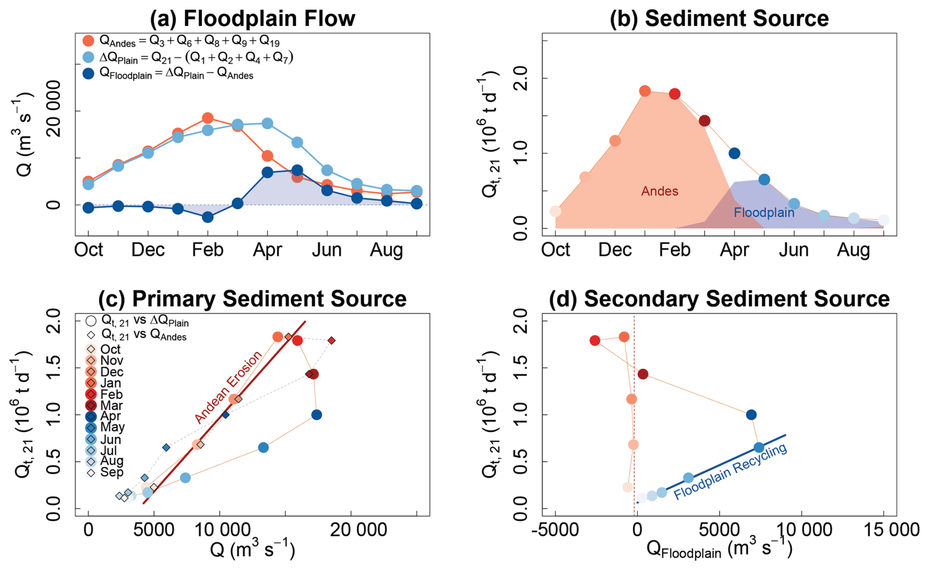
Figure 12Identification of sediment sources at the interannual scale. (a) Water discharge components: Andean Basin outflow (QAndes), basin outlet discharge excluding lateral contributions (ΔQplain) and floodplain flows (QFloodplain), all in m3 s−1. (b) Decomposition of total sediment flux at the basin outlet Qt,21 (106 t d−1) by sediment sources: red for Andean erosion, blue for floodplain recycling. (c) Relationship between Qt,21 and ΔQplain (circles) and QAndes (diamonds). The red regression line represents the relationship between QAndes and Qt,21 during rising limb months (d) Relationship between Qt,21 and QFloodplain. The blue regression line illustrates the relationship between QAndes and Qt,21 during recession months.
At the lowland outlet, discharge peaks two months after the Andes (April–May) delayed primarily by alluvial plain storage, diffusive flood wave propagation, and runoff from the northern part of the basin, where seasonality, driven by the South American monsoon system (Garreaud et al., 2009), is less pronounced than in the south. This upstream-to-downstream flooding dynamic leads to progressive floodplain inundation (February–April, Fig. 11b, c) and gradual drainage (March–July). Floodplain backflow (Fig. 12a) drives sediment remobilization from April to August (Fig. 12b, d). This secondary sediment source accounts for ∼ 22 % of the total suspended sediment load at the basin outlet and can have significant impacts on river dynamics, with pronounced effects during major floods (e.g., 2012, Fig. 6c). Floodplain flows, comprising precipitation, river inflows and backflows, are more significant than the water entering the floodplain from the main river (Fig. 12a), reinforcing the assumption that floodplain waters are blocked by the main channel during the rising limb.
In the following analysis, the fine sediment load of the Pachitea Basin was estimated using a rating curve derived from the relationship between water discharge and measured fine sediment load, based on simulated flows. For the other Andean sub-basins (8, 9, 3), fine sediment load was regionalized according to the drainage area of their respective Andean catchments. The Ucayali floodplain consists of three geomorphological compartments (Fig. 2b), each characterized by distinct processes:
Lagarto – Pucallpa (Box 1, Fig. 2b): A major thrust fault system involving the crystalline basement exerts significant tectonic control over the narrow sedimentary basin wedged between the young Shira Mountains and the Fitzcarrald Arch (Espurt et al., 2008; Pfiffner and Gonzalez, 2013; Gautheron et al., 2013). Here, 36 % of the 420 [386, 454] × 106 t yr−1 of Andean sediment accumulates, with sand deposition (−100 [−83, −117] × 106 t yr−1 ) accounting for 66 %. This results in alluvial plain aggradation at 3.7 mm yr−1 (9750 t km−2 yr−1), highlighting strong neotectonic control. In this compartment, water storage reaches 1.5 [1.1, 1.9] km3 in March on average, with flood durations (days with h ≥ hf) varying from 0 to 56 d in sub-basins 19 and 5, respectively. Consequently, daily-scale Andean flash floods superimposed on the annual monomodal flood wave are rapidly attenuated, while downstream, water storage increases as the floodplain expands. This process also dampens high-amplitude fine sediment peaks (−51 [−66, −35] × 106 t yr−1) through the activation of flood channels. These channels, remnants of the river's past mobility, further enhance the buffering effect. The sudden floodplain expansion at sub-basin 14 as the river course is released from the tectonic constraint imposed by the Shira Mountains reduces fine sediment loads (Fig. 11d), while high meander migration rates (Li et al., 2023) indicate active lateral erosion and deposition.
Pucallpa – Contaya Arch (Box 2, Fig. 2b). This section is a large piggyback basin located between the Andean wedge top and the Moa Divisor thrust fault system, with increased floodplain storage and longer flood durations (78–125 d). In March, it retains 10.4 [8.3, 12.5] km3 of water (∼ 20 % of discharge). Fine sediment load increases by +10 [+2, +17] × 106 t yr−1 due to Andean inputs, mainly from the Pachitea sub-basin, where one of the major Andean precipitation hotspots drives intense erosion rates (∼ 4,020 t km−2 yr−1, ∼ 1.5 mm yr−1 ). Similarly, sands show a slight increase of +4 [+1, +7] × 106 t yr−1 after accounting for Andean lateral inputs, resulting in a total flux increase of +14 [+3, +24] × 106 t yr−1. Floodplain drainage and sediment resuspension gain importance in this segment.
Contaya Arch – Requena (Box 3, Fig. 2b). The river shifts northeastward into the extensive Marañón Foredeep, a tectonic funnel terminating at the Iquitos Arch. In April, water storage reaches 9.4 [7.7, 11.1] km3 . The maximum flood duration reaches 125 d. The flood impacts both fine sediments and sands (Fig. 11), however with different processes. Fine sediment deposition (−16 [−23, −10] × 106 t yr−1, 7 % of the load) is driven by prolonged floodplain residence time, while sand sedimentation (−11 [−13, −9] × 106 t yr−1) results from energy dissipation when the floodplain is active. This process, never documented before in Amazonian rivers, captures approximately 14 % [10 %, 20 %] of the sand flux.
Overall basin budget. Integrating these three compartments, the Ucayali floodplain traps 165 [138, 192] × 106 t yr−1 of the 455 [410, 500] × 106 t yr−1 supplied by the Andes (∼ 36 %), with sand accounting for 65 % of total deposition. The downstream export to the Amazon River reaches 290 [235, 345] × 106 t yr−1 (26 % sand), identifying the Ucayali as the dominant sediment source among Andean foreland tributaries of the Amazon, exceeding the Marañón (∼ 144–173 × 106 t yr−1; Armijos et al., 2013) and the Beni (∼ 133 × 106 t yr−1; Vauchel et al., 2017). It also exhibits some of the highest specific erosion and deposition rates in the foreland. Net fine sediment loss across the basin amounts to 21 % of the Andean input, driven primarily by the dampening of Andean flash floods in Compartment 1. Floodplain recycling during the recession limb contributes approximately 22 % of the total suspended load at the basin outlet, acting as a secondary sediment source that partially offsets net deposition and sustains sediment export during the low-water season. Peak floodplain water storage reaches 19.1 [15.3, 22.9] km3 in March, equivalent to ∼ 38 % of total basin discharge for that month.
6.4.2 Long-term trends
No significant trends were observed in flood duration, floodplain water volume, discharge extremes, or sediment fluxes in sub-basins 21, 22, and 23 for the simulation period. This suggests that the effects of global and regional changes at the Ucayali Basin scale are still negligible, contrasting with studies of the broader Amazon Basin (e.g. Marengo, 2004; Gloor et al., 2013; Li et al., 2020; Fleischmann et al., 2023). However, most of these studies focus on a very limited number of sites with long-term data. This highlights the relevance of the integrated approach proposed in this study for generating new long-term analyses of regional trends and providing a more detailed perspective on the Amazon's response to global changes. Espinoza et al. (2009) is the only study on Ucayali discharge evolution, based on inconsistent 1996–2005 data, now curated here. Figueiredo et al. (2024) and Polasky et al. (2025) identified mixed precipitation trends in the Ucayali Basin, respectively for the 1982–2023 and 1980–2022 period, which may explain the lack of clear trends here. Nevertheless, Guimberteau et al. (2013, 2017) project increased precipitation in the western Amazon by the century's end, potentially leading to greater inundations, sediment deposition, and floodplain recycling, which may alter river mobility, particularly during extreme events. This could impact bedload transport, leading to bed aggradation, which would facilitate overflow and then intensify exchanges.
6.4.3 Implications for sediment routing in large floodplain river systems
The floodplain-controlled sand sedimentation process identified here, whereby inundation reduces main-channel transport capacity and captures ∼ 14 % of the sand flux at peak discharge, generating a secondary sediment peak during recession, has implications beyond the Ucayali Basin. Large tropical river systems draining tectonically active forelands onto extensive alluvial plains are likely to exhibit similar morphological conditions, suggesting that floodplain-driven decoupling of sand flux from water discharge may occur more broadly. The integrated approach developed here provides a framework to identify and quantify this process in other poorly monitored basins.
Three core findings emerge from this study.
First, floodplain inundation exerts a dual control on sediment dynamics: it captures ∼ 14 % [10 %, 20 %] of the sand flux at peak discharge by reducing main-channel transport capacity, while recycling processes during recession contribute 22 % of the total suspended load at the basin outlet. This floodplain-driven decoupling of sand flux from water discharge, previously undocumented in large Amazonian rivers, suggests that conventional approaches assuming a stationary relationship between water discharge and sand flux may overlook a first-order process in large floodplain river systems.
Second, the integrated framework developed here enables the first long-term hydro-sedimentary budgets for the Upper Amazon at sub-basin scale. The Andean Ucayali exports 455 [410, 500] × 106 t yr−1 of suspended sediment (40 % sand), of which 36 % is trapped within the floodplain, predominantly as sand (65 % of total deposition). Floodplain recycling contributes 22 % of the outlet load, and the Ucayali ultimately delivers 290 [235, 345] × 106 t yr−1 to the Amazon River (26 % sand), identifying the Ucayali as the dominant sediment source among Andean foreland tributaries of the Amazon. These estimates are stable over the 20–37-year record, with no significant long-term trends detected.
Third, in large floodplain rivers, the accuracy of sediment budgets is controlled by the sustained availability of multi-variable field observations at super stations, not primarily by model structure or parameter calibration. Despite substantial equifinality among secondary floodplain parameters, flux, trapping and recycling fractions remain stable across all behavioural GLUE simulations, demonstrating that long-term critical zone observatories such as HyBAm provide the irreducible constraint that no model refinement can substitute.
These findings highlight the need to rethink hydrological network operations through the concepts of super and virtual stations, combining long-term, high-quality in situ data with satellite measurements to constrain this integrated approach. Synchronizing targeted hydro-sedimentary gauging campaigns with satellite missions would significantly enhance model performance.
Moreover, the study underscores the importance of regionally focused and long-term analyses over broad, continental-scale assessments, which often introduce high uncertainties and may misguide sustainable development and mitigation strategies.
Looking ahead, this framework can be extended to other Amazonian basins facing similar hydro-sedimentary monitoring challenges, through targeted calibration campaigns and model refinements. The progressive deployment of satellite missions, particularly SWOT and Sentinel-3 for water levels and Sentinel-2 for high-resolution surface reflectance, will further enhance its spatial applicability by providing key constraints to calibrate floodplain activation thresholds and fine sediment concentrations in ungauged reaches.
The assimilation of satellite-derived fine sediment concentrations would significantly improve floodplain modelling by defining Floodplain Hydrological Response Units based on morphology (lakes, channels, etc.). By reconciling fine sediment mass balances (i.e., adjusting discrepancies between modelled and observed satellite data), this method would provide a proxy for water residence time in floodplains. This key variable is critical for constraining biogeochemical processes and could support the development of coupled bio-hydro-geochemical models, improving our understanding of the Amazon's role in global biogeochemical cycles and its response to environmental changes.
In conclusion, this study demonstrates that floodplains are not passive components of large river systems but active regulators of sediment transport, storage, and recycling. By integrating remote sensing, modelling, and long-term field observations, it provides a robust and scalable framework to quantify these processes, with implications for understanding biogeochemical cycles and managing large river basins under environmental change.
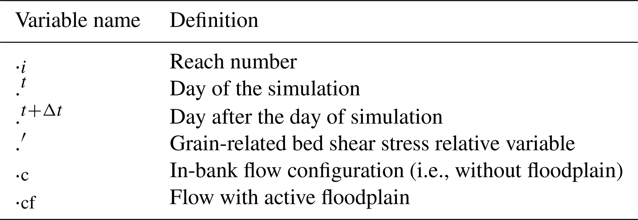
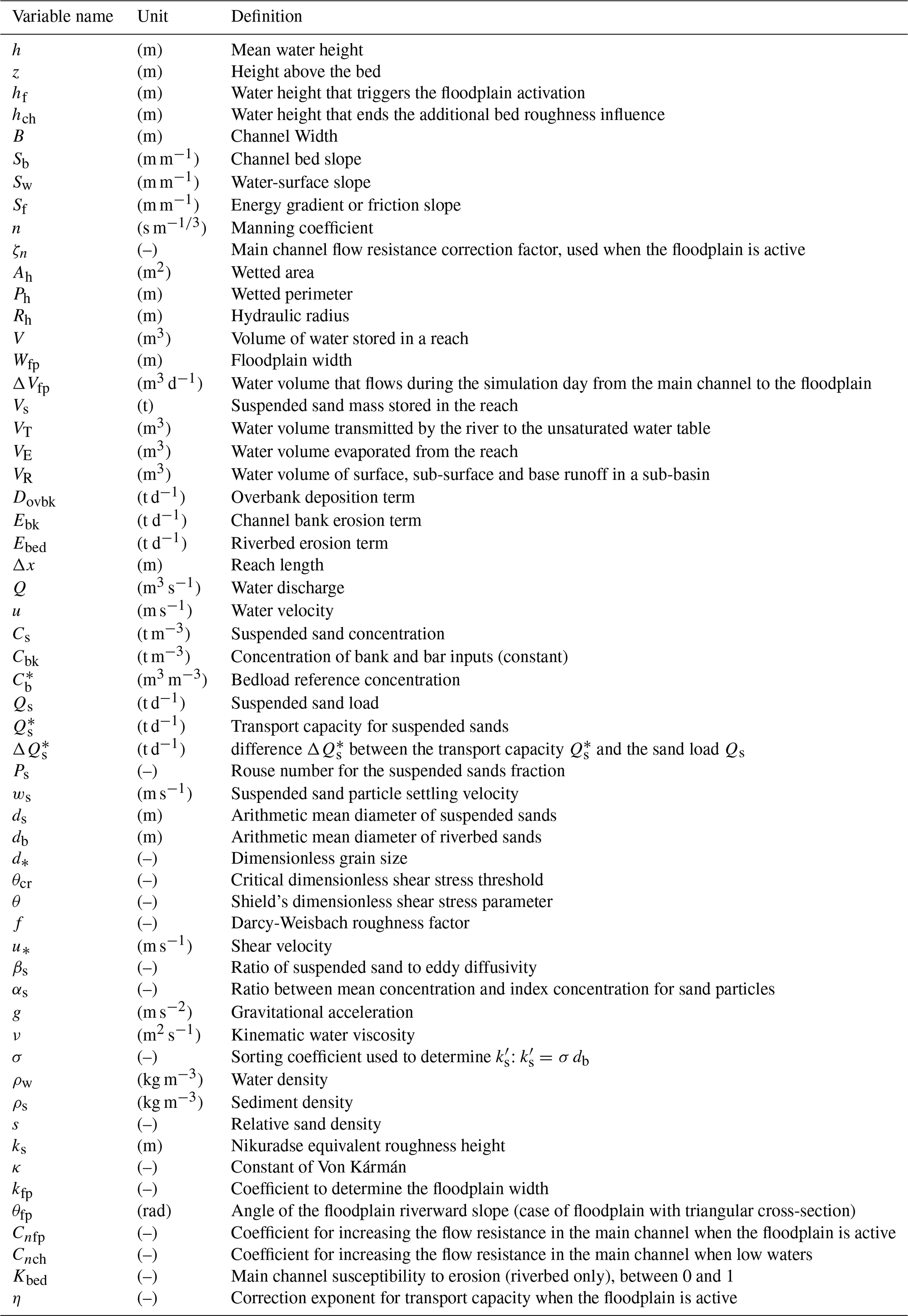
The R notebook used to run, calibrate, and analyze the SWAT-Amazon simulations, along with the SWAT-Amazon executable file, are openly available at: https://github.com/william-santini/SWAT-Amazon (last access: 6 June 2025) and are archived at https://doi.org/10.5281/zenodo.20414628 (Santini, 2025). Access to the SWAT-Amazon Fortran source code can be provided by the corresponding author upon reasonable request to ensure appropriate use and reproducibility. The data supporting the findings of this study are available from the corresponding author upon reasonable request and are partly accessible through the CZO HYBAM observatory website: https://hybam.obs-mip.fr (last access: 6 June 2025).
The supplement related to this article is available online at https://doi.org/10.5194/hess-30-3367-2026-supplement.
Conceptualization: WS. Methodology: WS. Software: WS, ADY. Investigation: WS. Formal analysis: WS. Data curation (conventional dataset): WS. Data curation (remote sensing dataset): WS, JR. Resources: WS, JJPA, WLC. Supervision: WS. Project administration: WS, JMM, WLC. Funding acquisition: JMM, WS, WLC. Writing – original draft: WS. Writing – review and editing: WS, BC, JR, WLC, JMC, JMM. Visualization: WS, ADY.
The contact author has declared that none of the authors has any competing interests.
Publisher's note: Copernicus Publications remains neutral with regard to jurisdictional claims made in the text, published maps, institutional affiliations, or any other geographical representation in this paper. The authors bear the ultimate responsibility for providing appropriate place names. Views expressed in the text are those of the authors and do not necessarily reflect the views of the publisher.
The authors would like to express their special thanks to their colleagues at the Peruvian National Service of Hydrology and Meteorology (SENAMHI) for preparing the PISCO precipitation and temperature datasets used in this study and to Marco Antonio Paredes, director of the zonal directorate of Loreto. Special thanks are also extended to Bruno Lartiges and Raul Espinoza-Villar for their support during the calibration campaigns.
This research was supported by the French National Research Institute for Sustainable Development (IRD), the National Center for Scientific Research (CNRS), and the Peruvian National Service of Hydrology and Meteorology (SENAMHI).
This paper was edited by Fabrizio Fenicia and reviewed by two anonymous referees.
Alfieri, L., Bisselink, B., Dottori, F., Naumann, G., de Roo, A., Salamon, P., Wyser, K., and Feyen, L.: Global projections of river flood risk in a warmer world, Earth's Future, 5, 171–182, https://doi.org/10.1002/2016EF000485, 2017.
Allen, P. A.: From landscapes into geological history, Nature, 451, 274–276, https://doi.org/10.1038/nature06586, 2008.
Armijos, E., Crave, A., Vauchel, P., Fraizy, P., Santini, W., Moquet, J. S., Arevalo, N., Carranza, J., and Guyot, J.: Suspended sediment dynamics in the Amazon River of Peru, J. South Am. Earth Sci., 44, 75–84, https://doi.org/10.1016/j.jsames.2012.09.002, 2013.
Arnold, J. G., Srinivasan, R., Muttiah, R. S., and Williams, J. R.: Large area hydrologic modeling and assessment: Part I – Model development of a basin-scale model called SWAT (Soil and Water Assessment Tool), Water Resour. Res., 34, 73–89, https://doi.org/10.1111/j.1752-1688.1998.tb05961.x, 1998.
Atabay, S. and Knight, D. W.: Effects of overbank flow on fluvial sediment transport rates, Inst. Civ. Eng. Proc. Water Marit. Eng., 158, 25–36, https://doi.org/10.1680/wama.158.1.25.62456, 2018.
Aufdenkampe, A. K., Mayorga, E., Raymond, P. A., Melack, J. M., Doney, S. C., Alin, S. R., Aalto, R. E., and Yoo, K.: Riverine coupling of biogeochemical cycles between land, oceans, and atmosphere, Front. Ecol. Environ., 9, 53–60, https://doi.org/10.1890/100014, 2011.
Aybar, C., Fernández, C., Huerta, A., Lavado, W., Vega, F., and Felipe-Obando, O.: Construction of a high-resolution gridded rainfall dataset for Peru from 1981 to the present day, Hydro. Sci. J., 65, 770–785, https://doi.org/10.1080/02626667.2019.1649411, 2020.
Baby, P. and Guyot, J.: Tectonic control of erosion and sedimentation in the Amazon Basin of Bolivia, Hydrol. Process., 23, 3225–3229, https://doi.org/10.1002/hyp.7391, 2009.
Bartholdy, J., Flemming, B. W., Ernstsen, V. B., Winter, C., and Bartholomä, A.: Hydraulic roughness over simple subaqueous dunes, Geo-Mar. Lett., 30, 63–76, https://doi.org/10.1007/s00367-009-0153-7, 2010.
Bates, P. D., Horritt, M. S., and Fewtrell, T. J.: A simple inertial formulation of the shallow water equations for efficient two-dimensional flood inundation modelling, J. Hydrol., 387, 33–45, https://doi.org/10.1016/j.jhydrol.2010.03.027, 2010.
Beven, K. J. and Binley, A.: The future of distributed models: model calibration and uncertainty prediction, Hydrol. Process., 6, 279–298, https://doi.org/10.1002/hyp.3360060305, 1992.
Bouchez, J., Gaillardet, J., Lupker, M., Louvat, P., France-Lanord, C., Maurice, L., Armijos, E., and Moquet, J. S.: Floodplains of large rivers: Weathering reactors or simple silos?, Chem. Geol., 332–333, 166–184, https://doi.org/10.1016/j.chemgeo.2012.09.032, 2012.
Bousmar, D. and Zech, Y.: Momentum transfer for practical flow computation in compound channels, J. Hydraul. Eng., 125, 696–706, https://doi.org/10.1061/(ASCE)0733-9429(1999)125:7(696), 1999.
Callède, J., Cochonneau, G., Alves, F. V., Guyot, J.-L., Guimarães, V. S., and De Oliveira, E.: The River Amazon water contribution to the Atlantic Ocean, Rev. Sci. Eau., 23, 247–273, https://doi.org/10.7202/044688ar, 2010.
Calmant, S., Seyler, F., and Cretaux, J. F.: Monitoring Continental Surface Waters by Satellite Altimetry, Surv. Geophys., 29, 247–269, https://doi.org/10.1007/s10712-008-9051-1, 2009.
Camenen, B. and Larson, M.: A general formula for non-cohesive bed load sediment transport, Estuar. Coast. Shelf Sci., 63, 249–260, https://doi.org/10.1016/j.ecss.2004.10.019, 2005.
Camenen, B. and Larson, M.: A general formula for noncohesive suspended sediment transport, J. Coast. Res., 243, 615–627, https://doi.org/10.2112/06-0694.1, 2008.
Camenen, B., Coz, J. Le, Dramais, G., Peteuil, C., Fretaud, T., Falgon, A., Dussouillez, P., and Moore, S. A.: A simple physically-based model for predicting sand transport dynamics in the Lower Mekong River, River Flow, 2189–2197, https://doi.org/10.1201/b17133-293, 2014.
Chaudhari, S. and Pokhrel, Y.: Alteration of River Flow and Flood Dynamics by Existing and Planned Hydropower Dams in the Amazon River Basin, Water Resour. Res., 58, https://doi.org/10.1029/2021WR030555, 2022.
Davidson, E. A., De Araújo, A. C., Artaxo, P., Balch, J. K., Brown, I. F., Mercedes, M. M., Coe, M. T., Defries, R. S., Keller, M., Longo, M., Munger, J. W., Schroeder, W., Soares-Filho, B. S., Souza, C. M., and Wofsy, S. C.: The Amazon basin in transition, Nature, 481, 321–328, https://doi.org/10.1038/nature10717, 2012.
Doxaran, D., Froidefond, J. M., Lavender, S., and Castaing, P.: Spectral signature of highly turbid waters: Application with SPOT data to quantify suspended particulate matter concentrations, Remote Sens. Environ., 81, 149–161, https://doi.org/10.1016/S0034-4257(01)00341-8, 2002.
Dramais, G.: Observation et modélisation des flux de sable dans les grands cours d'eau, PhD thesis, University of Lyon, https://theses.hal.science/tel-03188258 (last access: 6 June 2025), 2020.
Dunne, T., Mertes, L. A. K., Meade, R. H., Richey, J. E., and Forsberg, B. R.: Exchanges of sediment between the flood plain and channel of the Amazon River in Brazil, Geol. Soc. Am. Bull., 110, 450–467, https://doi.org/10.1130/0016-7606(1998)110<0450:EOSBTF>2.3.CO;2, 1998
Einstein, H. A.: The Bed-Load Function for Sediment Transportation in Open Channel Flows, Technical Bulletins 156389, United States Department of Agriculture, Economic Research Service, https://doi.org/10.22004/ag.econ.156389, 1950.
Einstein, H. A. and Barbarossa, N. L.: River Channel Roughness, Trans. Am. Soc. Civ. Eng., 117, 1121–1146, https://doi.org/10.1061/TACEAT.0006666, 1952.
Engelund, F. and Hansen, E.: A Monograph on Sediment Transport in Alluvial Streams, Teknishforlag Technical Press, Copenhagen, https://resolver.tudelft.nl/uuid:81101b08-04b5-4082-9121-861949c336c9 (last access: 6 June 2025), 1967.
Ervine, D. A. and Baird, J. I.: Rating curves for rivers with overbank flow, Proc. Inst. Civ. Eng. Part 2 Res. Theory, 73, 465–472, https://doi.org/10.1680/iicep.1982.1712, 1982.
Espinoza, J. C., Guyot, J. L., Ronchail, J., Cochonneau, G., Filizola, N., Fraizy, P., Labat, D., De Oliveira, E., Ordoñez, J. J., and Vauchel, P.: Contrasting regional discharge evolutions in the Amazon basin (1974–2004), J. Hydrol., 375, 297–311, https://doi.org/10.1016/j.jhydrol.2009.03.004, 2009.
Espinoza, J. C., Ronchail, J., Guyot, J. L., Junquas, C., Drapeau, G., Martinez, J. M., Santini, W., Vauchel, P., Lavado, W., Ordoñez, J., and Espinoza-Villar, R.: From drought to flooding: understanding the abrupt 2010–11 hydrological annual cycle in the Amazonas River and tributaries, Environ. Res. Lett., 7, 024008, https://doi.org/10.1088/1748-9326/7/2/024008, 2012.
Espinoza, J. C., Ronchail, J., Guyot, J. L., Junquas, C., Vauchel, P., Lavado, W., Drapeau, G., and Pombosa, R.: Climate variability and extreme drought in the Upper Amazon basin, Hydrol. Process., 27, 1132–1143, 2013.
Espinoza-Villar, R., Martinez, J. M., Guyot, J. L., Fraizy, P., Armijos, E., Crave, A., Bazan, H., Vauchel, P., and Lavado, W.: The integration of field measurements and satellite observations to determine river solid loads in poorly monitored basins, J. Hydrol., 444–445, 221–228, https://doi.org/10.1016/j.jhydrol.2012.04.024, 2012.
Espinoza-Villar, R., Martinez, J. M., Le Texier, M., Guyot, J. L., Fraizy, P., Meneses, P. R., and De Oliveira, E.: A study of sediment transport in the Madeira River, Brazil, using MODIS remote-sensing images, J. S. Am. Earth Sci., 44, 45–54, https://doi.org/10.1016/j.jsames.2012.11.006, 2013.
Espinoza-Villar, R., Martinez, J. M., Armijos, E., Espinoza, J. C., Filizola, N., Dos Santos, A., Willems, B., Fraizy, P., Santini, W., and Vauchel, P.: Spatio-temporal monitoring of suspended sediments in the Solimões River (2000–2014), C. R. Geosci., 349, 4–12, https://doi.org/10.1016/j.crte.2017.05.001, 2017.
Espurt, N., Brusset, S., Baby, P., Hermoza, W., Bolaños, R., Uyen, D., and Déramond, J.: Paleozoic structural controls on shortening transfer in the Subandean foreland thrust system, Ene and southern Ucayali basins, Peru, Tectonics, 27, TC3009, https://doi.org/10.1029/2007TC002238, 2008.
Fagundes, H. D. O., Cauduro Dias de Paiva, R., Mainardi Fan, F., Costa Buarque, D., and César Fassoni-Andrade, A.: Sediment modeling of a large-scale basin supported by remote sensing and in-situ observations, Catena, 190, 104535, https://doi.org/10.1016/j.catena.2020.104535, 2020.
Fagundes, H. D. O., Fan, F. M., Paiva, R. C. D., Buarque, D. C., Kornowski, L. W., Laipelt, L., and Collischonn, W.: Sediment flows in South America supported by daily hydrologic-hydrodynamic modeling, Water Resour. Res., 57, e2020WR027884, https://doi.org/10.1029/2020WR027884, 2021.
Fagundes, H. D. O., Fleischmann, A. S., Fan, F. M., Paiva, R. C. D., Buarque, D. C., and Siqueira, V. A.: Human-induced changes in South American river sediment fluxes from 1984 to 2019, Water Resour. Res., 59, e2023WR034519, https://doi.org/10.1029/2023WR034519, 2023.
Fan, Y. and Miguez-Macho, G.: Potential groundwater contribution to Amazon evapotranspiration, Hydrol. Earth Syst. Sci., 14, 2039–2056, https://doi.org/10.5194/hess-14-2039-2010, 2010.
Fleischmann, A. S., Papa, F., Fassoni-Andrade, A., Melack, J. M., Wongchuig, S., Paiva, R. C. D., Hamilton, S. K., Fluet-Chouinard, E., Barbedo, R., Aires, F., Al Bitar, A., Bonnet, M. P., Coe, M., Ferreira-Ferreira, J., Hess, L., Jensen, K., McDonald, K., Ovando, A., Park, E., Parrens, M., Pinel, S., Prigent, C., Resende, A. F., Revel, M., Rosenqvist, A., Rosenqvist, J., Rudorff, C., Silva, T. S. F., Yamazaki, D., and Collischonn, W.: How much inundation occurs in the Amazon River basin?, Remote Sens. Environ., 278, https://doi.org/10.1016/j.rse.2022.113099, 2022.
Fleischmann, A. S., Papa, F., Hamilton, S. K., Fassoni-Andrade, A., Wongchuig, S., Espinoza, J. C., Paiva, R. C. D., Melack, J. M., Fluet-Chouinard, E., Castello, L., Almeida, R. M., Bonnet, M. P., Alves, L. G., Moreira, D., Yamazaki, D., Revel, M., and Collischonn, W.: Increased floodplain inundation in the Amazon since 1980, Environ. Res. Lett., 18, https://doi.org/10.1088/1748-9326/acb9a7, 2023.
Figueiredo, D., Filho, F. C. F., and Pessoa, L.: Homogeneous regions of precipitation trends across the Amazon River Basin, determined from the Global Precipitation Climatology Centre, Rev. Bras. Meteorol., 39, 1283–1308, https://doi.org/10.26848/rbgf.v17.2.p1283-1308, 2024.
Finer, M. and Jenkins, C. N.: Proliferation of hydroelectric dams in the Andean Amazon and implications for Andes-Amazon connectivity, PLoS One, 7, e35126, https://doi.org/10.1371/journal.pone.0035126, 2012.
Fleming, K., Johnston, P., Zwartz, D., Yokoyama, Y., Lambeck, K., and Chappell, J.: Refining the eustatic sea-level curve since the Last Glacial Maximum using far- and intermediate-field sites, Earth Planet. Sci. Lett., 163, 327–342, https://doi.org/10.1016/S0012-821X(98)00198-8, 1998.
Flores, B. M., Montoya, E., Sakschewski, B., Nascimento, N., Staal, A., Betts, R. A., Levis, C., Lapola, D. M., Esquível-Muelbert, A., Jakovac, C., Nobre, C. A., Oliveira, R. S., Borma, L. S., Nian, D., Boers, N., Hecht, S. B., ter Steege, H., Arieira, J., Lucas, I. L., Berenguer, E., Marengo, J. A., Gatti, L. V., Mattos, C. R. C., and Hirota, M.: Critical transitions in the Amazon forest system, Nature, 626, 555–564, https://doi.org/10.1038/s41586-023-06970-0, 2024.
Gaillardet, J., Dupré, B., Louvat, P., and Allègre, C. J.: Global silicate weathering and CO2 consumption rates deduced from the chemistry of large rivers, Chem. Geol., 159, 3–30, https://doi.org/10.1016/S0009-2541(99)00031-5, 1999.
Garreaud, R. D., Vuille, M., Compagnucci, R., and Marengo, J.: Present-day South American climate, Palaeogeogr. Palaeoclimatol. Palaeoecol., 281, 180–195, https://doi.org/10.1016/j.palaeo.2007.10.032, 2009.
Gautheron, C., Espurt, N., Barbarand, J., Roddaz, M., and Baby, P.: Direct dating of thick- and thin-skin thrusts in the Peruvian Subandean zone through apatite (U–Th)/He and fission track thermochronometry, Basin Res., 419–435, https://doi.org/10.1111/bre.12012, 2013.
Gitto, A. B., Venditti, J. G., Kostaschuk, R., and Church, M.: Representative point-integrated suspended sediment sampling in rivers, Water Resour. Res., 53, 2956–2971, https://doi.org/10.1002/2016WR019742, 2017.
Gloor, M., Brienen, R. J. W., Galbraith, D., Feldpausch, T. R., Schöngart, J., Guyot, J., Espinoza, J. C., Lloyd, J., and Phillips, O. L.: Intensification of the Amazon hydrological cycle over the last two decades, Geophys. Res. Lett., 40, 1729–1733, https://doi.org/10.1002/grl.50377, 2013.
Guilhen, J., Parrens, M., Sauvage, S., Santini, W., Mercier, F., Al Bitar, A., Fabre, C., Martinez, J. M., and Sànchez-Pérez, J. M.: Estimation of the Madeira floodplain dynamics from 2008 to 2018, Front. Water., 4, https://doi.org/10.3389/frwa.2022.952810, 2022.
Guimberteau, M., Ronchail, J., Espinoza, J. C., Lengaigne, M., Sultan, B., Polcher, J., Drapeau, G., Guyot, J.-L., Ducharne, A., and Ciais, P.: Future changes in precipitation and impacts on extreme streamflow over Amazonian sub-basins, Environ. Res. Lett., 8, 014035, https://doi.org/10.1088/1748-9326/8/1/014035, 2013.
Guimberteau, M., Ciais, P., Ducharne, A., Boisier, J. P., Dutra Aguiar, A. P., Biemans, H., De Deurwaerder, H., Galbraith, D., Kruijt, B., Langerwisch, F., Poveda, G., Rammig, A., Rodriguez, D. A., Tejada, G., Thonicke, K., Von Randow, C., Von Randow, R. C. S., Zhang, K., and Verbeeck, H.: Impacts of future deforestation and climate change on the hydrology of the Amazon Basin: a multi-model analysis with a new set of land-cover change scenarios, Hydrol. Earth Syst. Sci., 21, 1455–1475, https://doi.org/10.5194/hess-21-1455-2017, 2017.
Guyot, J. Loup: Hydrogéochimie des fleuves de l'Amazonie bolivienne. PhD thesis, Paris: Editions de l'ORSTOM, https://horizon.documentation.ird.fr/exl-doc/pleins_textes/pleins_textes_2/etudes_theses/38760.pdf (last access: 6 June 2025), 1993.
Guyot, J., Jouanneau, J. M., Soares, L., Boaventura, G. R., Maillet, N., and Lagane, C.: Clay mineral composition of river sediments in the Amazon Basin, Catena, 71, 340–356, https://doi.org/10.1016/j.catena.2007.02.002, 2007.
Hager, W. H.: Gauckler et la formule d'écoulement uniforme, Houille Blanche, 3, 17–22, https://doi.org/10.1051/lhb:200503001, 2005.
Hargreaves, G. H. and Samani, Z. A.: Reference crop evapotranspiration from temperature, Appl. Eng. Agric., 1, 96–99, https://doi.org/10.13031/2013.26773, 1985.
Hess, L. L., Melack, J. M., Affonso, A. G., Barbosa, C. C. F., Gastil-Buhl, M., and Novo, E. M. L. M.: Wetlands of the Lowland Amazon Basin: Extent, Vegetative Cover, and Dual-season Inundated Area as Mapped with JERS-1 Synthetic Aperture Radar, Wetlands, 35, 745–756, https://doi.org/10.1007/s13157-015-0666-y, 2015.
Hirabayashi, Y., Mahendran, R., Koirala, S., Konoshima, L., Yamazaki, D., Watanabe, S., Kim, H., and Kanae, S.: Global flood risk under climate change, Nat. Clim. Chang., 3, 816–821, https://doi.org/10.1038/nclimate1911, 2013.
Horowitz, A. J., Clarke, R. T., and Merten, G. H.: The effects of sample scheduling and sample numbers on estimates of the annual fluxes of suspended sediment in fluvial systems, Hydrol. Process., 543, 531–543, https://doi.org/10.1002/hyp.10172, 2015.
Jouanno, J., Moquet, J. S., Berline, L., Radenac, M.-H., Santini, W., Changeux, T., Thibaut, T., Podlejski, W., Menard, F., Martinez, J. M., Aumont, O., Sheinbaum, J., Filizola, N., and Mounkandi N'kaya, G. D.: Evolution of the riverine nutrient export to the Tropical Atlantic over the last 15 years: is there a link with Sargassum proliferation?, Environ. Res. Lett., https://doi.org/10.1088/1748-9326/abe11a, 2021.
Knight, D. W.: Hydraulics of Flood Channels, in: Floods: Hydrological, Sedimentological and Geomorphological Implications, edited by: Beven, K. and Carling, P., John Wiley & Sons Ltd., Chichester, Royaume-Uni, ISBN 9780471921646, 1989.
Knight, D. W. and Shiono, K.: River channel and floodplain hydraulics, in: Floodplain Processes, edited by: Anderson, M. G., Walling, D. E., and Bates, P. D., Wiley, New York, 139–181, ISBN 9780471966791, 1996.
Langerwisch, F., Rost, S., Gerten, D., Poulter, B., Rammig, A., and Cramer, W.: Potential effects of climate change on inundation patterns in the Amazon Basin, Hydrol. Earth Syst. Sci., 17, 2247–2262, https://doi.org/10.5194/hess-17-2247-2013, 2013.
Latrubesse, E. M., Arima, E. Y., Dunne, T., Park, E., Baker, V. R., D'Horta, F. M., Wight, C., Wittmann, F., Zuanon, J., Baker, P. A., Ribas, C. C., Norgaard, R. B., Filizola, N., Ansar, A., Flyvbjerg, B., and Stevaux, J. C.: Damming the rivers of the Amazon basin, Nature, 546, 363–369, https://doi.org/10.1038/nature22333, 2017.
Lesack, L. F. W.: Water balance and hydrologic characteristics of a rain forest catchment in the central Amazon Basin, Water Resour. Res., 29, 759–773, https://doi.org/10.1029/92WR02371, 1993.
Lewin, J., Ashworth, P. J., Strick, R. J. P., and Nicholas, A. P.: Spillage sedimentation on large river floodplains, Earth Surf. Process. Landf., 42, 290–305, https://doi.org/10.1002/esp.3996, 2017.
Li, T., Wang, S., Liu, Y., Fu, B., and Gao, D.: Reversal of the sediment load increase in the Amazon basin influenced by divergent trends of sediment transport from the Solimões and Madeira Rivers, Catena, 195, 104804, https://doi.org/10.1016/j.catena.2020.104804, 2020.
Li, Z., Mendoza, A., Abad, J. D., Endreny, T. A., Han, B., Carrisoza, E., and Dominguez, R.: High-resolution modeling of meander neck cutoffs: laboratory and field scales, Front. Earth Sci., 11, 1–13, https://doi.org/10.3389/feart.2023.1208782, 2023.
Lininger, K. B. and Latrubesse, E. M.: Flooding hydrology and peak discharge attenuation along the middle Araguaia River in central Brazil, Catena, 143, 90–101, https://doi.org/10.1016/j.catena.2016.03.043, 2016.
Llauca, H., Lavado-Casimiro, W., Montesinos, C., Santini, W., and Rau, P.: PISCO_HyM_GR2M: A model of monthly water balance in Peru (1981–2020), Water, 13, 1048, https://doi.org/10.3390/w13081048, 2021.
Louchard, D., Gruber, N., and Münnich, M.: The Impact of the Amazon on the Biological Pump and the Air-Sea CO2 Balance of the Western Tropical Atlantic, Global Biogeochem. Cycles, 35, https://doi.org/10.1029/2020GB006818, 2021.
Louchard, D., Münnich, M., and Gruber, N.: On the Role of the Amazon River for N2 Fixation in the Western Tropical Atlantic, Global Biogeochem. Cycles, 37, https://doi.org/10.1029/2022GB007537, 2023.
Lovejoy, T. E. and Nobre, C.: Amazon tipping point: Last chance for action, Sci. Adv., 5, eaba2949, https://doi.org/10.1126/sciadv.aba2949, 2019.
Loveless, J. H., Sellin, R. H. J., Bryant, T. B., Wormleaton, P. R., Catmur, S., and Hey, R.: The effect of overbank flow in a meandering river on its conveyance and the transport of graded sediments, J. Char. Inst. Water Environ. Manag., 14, 447–455, https://doi.org/10.1111/j.1747-6593.2000.tb00293.x, 2000.
Malhi, Y., Roberts, J. T., Betts, R. A., Killeen, T. J., Li, W., and Nobre, C. A.: Climate change, deforestation, and the fate of the Amazon, Science, 319, 169–172, https://doi.org/10.1126/science.1146961, 2008.
Marengo, J. A.: Interdecadal variability and trends of rainfall across the Amazon basin, Theor. Appl. Climatol., 78, 79–96, https://doi.org/10.1007/s00704-004-0045-8, 2004.
Marengo, J. A. and Espinoza, J. C.: Extreme seasonal droughts and floods in Amazonia: Causes, trends and impacts, Int. J. Climatol., 35, 1033–1050, https://doi.org/10.1002/joc.4420, 2016.
Martinelli, A. L. R. dos S.: Análise temporal e espacial dos dados de sedimentos em estações hidrométricas na Amazônia: casos de Manacapuru e Itacoatiara, Ph.D. thesis, Programa de Pós-Graduação em Clima e Ambiente – Cliamb, Instituto Nacional de Pesquisas da Amazônia (INPA), Manaus, Brésil, https://rigeo.cprm.gov.br/jspui/handle/doc/22918 (last access: 6 June 2025), 2022.
Martinez, J. M., Guyot, J., Filizola, N., and Sondag, F.: Increase in suspended sediment discharge of the Amazon River assessed by monitoring network and satellite data, Catena, 79, 257–264, https://doi.org/10.1016/j.catena.2009.05.011, 2009.
Martinez, J. M., Espinoza-Villar, R., Armijos, E., and Moreira, L. S.: The optical properties of river and floodplain waters in the Amazon River Basin: Implications for satellite-based measurements of suspended particulate matter, J. Geophys. Res. Earth Surf., 120, 1–14, https://doi.org/10.1002/2014JF003404, 2015.
McKay, D. I. A., Staal, A., Abrams, J. F., Winkelmann, R., Sakschewski, B., Loriani, S., Fetzer, I., Cornell, S. E., Rockström, J., and Lenton, T. M.: Exceeding 1.5 °C global warming could trigger multiple climate tipping points, Science, 377, https://doi.org/10.1126/science.abn7950, 2022.
McQuarrie, N.: Initial plate geometry, shortening variations, and evolution of the Bolivian orocline, Geology, 30, 867, https://doi.org/10.1130/0091-7613(2002)030<0867:IPGSVA>2.0.CO;2, 2002a.
McQuarrie, N.: The kinematic history of the central Andean fold-thrust belt, Bolivia: Implications for building a high plateau, Geol. Soc. Am. Bull., 114, 950–963, https://doi.org/10.1130/0016-7606(2002)114<0950:TKHOTC>2.0.CO;2, 2002b.
Meade, R. H., Dunne, T., Richey, J. E., Santos de M., U., and Salati, E.: Storage and Remobilization of Suspended Sediment in the Lower Amazon River of Brazil, Science, 228, 488–490, https://doi.org/10.1126/science.228.4698.488, 1985.
Melack, J. M., Hess, L. L., Gastil, M., Forsberg, B. R., Hamilton, S. K., Lima, I. B. T., and Novo, E. M. L. M.: Regionalization of methane emissions in the Amazon Basin with microwave remote sensing, Glob. Chang. Biol., 10, 530–544, https://doi.org/10.1111/j.1365-2486.2004.00763.x, 2004.
Mertes, L. A. K., Dunne, T., and Martinelli, L. A.: Channel-floodplain geomorphology along the Solimões-Amazon River, Brazil, Geol. Soc. Am. Bull., 108, 1089–1107, https://doi.org/10.1130/0016-7606(1996)108{%}3C1089:cfgats{%}3E2.3.co;2, 1996.
Mobley, C. D.: Estimation of the remote-sensing reflectance from above-surface measurements, Appl. Opt., 38, 7442–7455, https://doi.org/10.1364/AO.38.007442, 1999.
Montgomery, D. R., Balco, G., and Willett, S. D.: Climate, tectonics, and the morphology of the Andes, Geology, 29, 579–582, 2001.
Moquet, J. S., Guyot, J. L., Crave, A., Viers, J., Filizola, N., Martinez, J. M., Oliveira, T. C., Sánchez, L. S. H., Lagane, C., Casimiro, W. S. L., Noriega, L., and Pombosa, R.: Amazon River dissolved load: temporal dynamics and annual budget from the Andes to the ocean, Environ. Sci. Pollut. Res., 23, 11405–11429, https://doi.org/10.1007/s11356-015-5503-6, 2016.
Moreira-Turcq, P., Bonnet, M., Amorim, M., Bernardes, M., Lagane, C., Maurice, L., Perez, M., and Seyler, P.: Seasonal variability in concentration, composition, age, and fluxes of particulate organic carbon exchanged between the floodplain and Amazon River, Geophys. Res. Lett.: Biogeosciences, 27, 119–130, https://doi.org/10.1002/gbc.20022, 2013.
Moriasi, D. N., Arnold, J. G., Van Liew, M. W., Binger, R. L., Harmel, R. D., and Veith, T. L.: Model evaluation guidelines for systematic quantification of accuracy in watershed simulations, Trans. Am. Soc. Agric. Eng., 50, 885–900, https://doi.org/10.13031/2013.23153, 2007.
Moussa, R. and Bocquillon, C.: On the use of the diffusive wave for modelling extreme flood events with overbank flow in the floodplain, J. Hydrol., 374, 116–135, https://doi.org/10.1016/j.jhydrol.2009.06.006, 2009.
Nobre, C. A., Sampaio, G., Borma, L. S., Castilla-Rubio, J. C., Silva, J. S., and Cardoso, M.: Land-use and climate change risks in the Amazon and the need of a novel sustainable development paradigm, Proc. Natl. Acad. Sci. USA, 113, 10759–10768, https://doi.org/10.1073/pnas.1605516113, 2016.
Paiva, R. C. D., Buarque, D. C., Collischonn, W., Bonnet, M.-P., Frappart, F., Calmant, S., and Bulhões Mendes, C. A.: Large-scale hydrologic and hydrodynamic modeling in South America, Water Resour. Res., 49, 1226–1243, https://doi.org/10.1002/wrcr.20067, 2013.
Pangala, S. R., Enrich-Prast, A., Basso, L. S., Peixoto, R. B., Bastviken, D., Hornibrook, E. R. C., Gatti, L. V., Marotta, H., Calazans, L. S. B., and Richey, J. E.: Large emissions from floodplain trees close the Amazon methane budget, Nature, 552, 230–234, https://doi.org/10.1038/nature24639, 2017.
Park, E. and Latrubesse, E. M.: Modeling suspended sediment distribution patterns of the Amazon River using MODIS data, Remote Sens. Environ., 147, 232–242, https://doi.org/10.1016/j.rse.2014.03.013, 2014.
Park, E. and Latrubesse, E. M.: The hydro-geomorphologic complexity of the lower Amazon River floodplain and hydrological connectivity assessed by remote sensing and field control, Remote Sens. Environ., 198, 321–332, https://doi.org/10.1016/j.rse.2017.06.021, 2017.
Pfiffner, O. and Gonzalez, L.: Mesozoic–Cenozoic evolution of the Western Margin of South America: Case study of the Peruvian Andes, Geosciences, 3, 262–310, https://doi.org/10.3390/geosciences3020262, 2013.
Pinet, S.: Analyse et caractérisation par télédétection des eaux de surfaces continentales pour l'étude des flux de matières: apport de l'analyse hyperspectrale et de la modélisation bio-optique, PhD thesis, Université Toulouse III – Paul Sabatier, Toulouse, France,https://theses.fr/2017TOU30124 (last access: 6 June 2025), 2017.
Polasky, A., Sapkota, V., Forest, C. E., and Fuentes, J. D.: Discrepancies in precipitation trends between observational and reanalysis datasets in the Amazon Basin, Sci. Rep., 15, 1–12, https://doi.org/10.1038/s41598-025-87418-5, 2025.
Pontes, P., Fan, F. M., Fleischmann, A. S., de Paiva, R. C. D., Buarque, D. C., Siqueira, V. A., Jardim, P. F., Sorribas, M. V., and Collischonn, W.: MGB-IPH model for hydrological and hydraulic simulation of large floodplain river systems coupled with open source GIS, Environ. Model. Softw., 94, 1–20, https://doi.org/10.1016/j.envsoft.2017.03.029, 2017.
Proust, S. and Nikora, V. I.: Compound open-channel flows: effects of transverse currents on the flow structure, J. Fluid Mech., 885, A24, https://doi.org/10.1017/jfm.2019.973, 2020.
Richey, J. E., Mertes, L. A. K., Dunne, T., Victoria, R. L. F., Forsberg, B. R., Tancredi, A. C. N. S., and Oliveira, E.: Sources and routing of the Amazon River Flood Wave, Global Biogeochem. Cycles, 3, 191–204, https://doi.org/10.1029/GB003i003p00191, 1989.
Richey, J. E., Melack, J. M., Aufdenkampe, A. K., Ballester, V. M., and Hess, L. L.: Amazon River flood dynamics: hydrological controls and biological consequences, Global Biogeochem. Cycles, 16, 6413–6416, https://doi.org/10.1038/416617a, 2002.
Rouse, H.: Modern conceptions of the mechanics of fluid turbulence, Trans. Am. Soc. Civ. Eng., 102, 463–505, https://doi.org/10.1061/TACEAT.0004872, 1937.
Rudorff, C. M., Melack, J. M., and Bates, P. D.: Flooding dynamics on the lower Amazon floodplain: 1. Hydraulic controls on water elevation, inundation extent, and river-floodplain discharge, Water Resour. Res., 50, 619–634, https://doi.org/10.1002/2013WR014091, 2014a.
Rudorff, C. M., Melack, J. M., and Bates, P. D.: Flooding dynamics on the lower Amazon floodplain: 2. Seasonal and interannual hydrological variability, Water Resour. Res., 50, 635–649, https://doi.org/10.1002/2013WR014714, 2014b.
Salati, E.: The role of water in the Amazon Basin: An isotopic study, Water Resour. Res., 15, 1250–1258, https://doi.org/10.1029/wr015i005p01250, 1979.
Santini, W.: Caractérisation de la dynamique hydro-sédimentaire du bassin de l'Ucayali (Pérou), par une approche intégrant réseau de mesures, télédétection et modélisation hydrologique, PhD thesis, Université Toulouse III – Paul Sabatier, Toulouse, France, https://theses.fr/2020TOU30276 (last access: 6 June 2025), 2020.
Santini, W.: SWAT-Amazon: R notebook and executable for running, calibrating, and analyzing SWAT-Amazon simulations, Zenodo [code], https://doi.org/10.5281/zenodo.20414628, 2025.
Santini, W., Martinez, J. M., Espinoza-Villar, R., Cochonneau, G., Vauchel, P., Moquet, J. S., Baby, P., Espinoza, J. C., Lavado, W., Carranza, J., and Guyot, J.: Sediment budget in the Ucayali River basin, an Andean tributary of the Amazon River, IAHS-AISH Proc. Reports, 367, 320–325, https://doi.org/10.5194/piahs-367-320-2015, 2014.
Santini, W., Camenen, B., Le Coz, J., Vauchel, P., Guyot, J.-L., Lavado, W., Carranza, J., Paredes, M. A., Pérez Arévalo, J. J., Arévalo, N., Espinoza Villar, R., Julien, F., and Martinez, J.-M.: An index concentration method for suspended load monitoring in large rivers of the Amazonian foreland, Earth Surf. Dyn., 7, 515–536, https://doi.org/10.5194/esurf-7-515-2019, 2019.
Satyamurty, P., Costa, C. P. W., Manzi, A. O., and Tavares Corrêa, F.: Moisture source for the Amazon Basin: A study of contrasting years, Theor. Appl. Climatol., 111, 195–209, https://doi.org/10.1007/s00704-012-0637-7, 2013.
Schürz, C.: SWATplusR: Running SWAT2012 and SWAT+ Projects in R, R package version 0.2.7, Zenodo [code], https://doi.org/10.5281/zenodo.3373859, 2019.
Sellin, R. H. J.: Interaction between the flow in the channel of a river and that over its flood plain, Houille Blanche, 7, 793–802, https://doi.org/10.1051/lhb/1964044, 1964.
Siqueira, V. A., Paiva, R. C. D., Fleischmann, A. S., Fan, F. M., Ruhoff, A. L., Pontes, P. R. M., Paris, A., Calmant, S., and Collischonn, W.: Toward continental hydrologic–hydrodynamic modeling in South America, Hydrol. Earth Syst. Sci., 22, 4815–4842, https://doi.org/10.5194/hess-22-4815-2018, 2018.
Smart, G. M.: Stage-discharge discontinuity in composite flood channels, J. Hydraul. Res., 30, 817–833, https://doi.org/10.1080/00221689209498912, 1992.
Soares-Filho, B., Moutinho, P., Nepstad, D., Anderson, A., Rodrigues, H., Garcia, R., Dietzsch, L., Merry, F., Bowman, M., Hissa, L., Silvestrini, R., and Maretti, C.: Role of Brazilian Amazon protected areas in climate change mitigation, Proc. Natl. Acad. Sci. USA, 107, 10821–10826, https://doi.org/10.1073/pnas.0913048107, 2010.
Sorribas, M. V., Paiva, R. C. D., Melack, J. M., Bravo, J. M., Jones, C., Carvalho, L., Beighley, E., and Forsberg, B.: Projections of climate change effects on discharge and inundation in the Amazon basin, Clim. Change, 136, 555–570, https://doi.org/10.1007/s10584-016-1640-2, 2016.
Soulsby, R. L.: Dynamics of Marine Sands: A Manual for Practical Applications, Thomas Telford, London, UK, ISBN 0-7277-2584-X, 1997.
Subramaniam, A., Yager, P. L., Carpenter, E. J., Mahaffey, C., Björkman, K., Cooley, S., Kustka, A. B., McManus, J. P., Sañudo-Wilhelmy, S. A., Schroeder, W., and Schroeder, W.: Amazon River enhances diazotrophy and carbon sequestration in the tropical North Atlantic Ocean, Proc. Natl. Acad. Sci. USA, 105, 10460–10465, https://doi.org/10.1073/pnas.0710279105, 2008.
Syvitski, J. P., Vörösmarty, C. J., Kettner, A. J., and Green, P.: Impact of Humans on the Flux of Terrestrial Sediment to the Global Coastal Ocean, Science, 308, 376–380, https://doi.org/10.1126/science.1109454, 2005.
Timpe, K. and Kaplan, D.: The changing hydrology of a dammed Amazon, Sci. Adv., 3, 1–13, https://doi.org/10.1126/sciadv.1700611, 2017.
Towner, J., Cloke, H. L., Lavado, W., Santini, W., Bazo, J., Coughlan de Perez, E., and Stephens, E. M.: Attribution of Amazon floods to modes of climate variability: A review, Meteorol. Appl., 27, https://doi.org/10.1002/met.1949, 2020.
Tricart, J.: Types de lits fluviaux en Amazonie brésilienne, Ann. géogr,, 86, 1–54, 1977.
Trigg, M. A., Wilson, M. D., Bates, P. D., Horritt, M. S., Alsdorf, D. E., Forsberg, B. R., and Vega, M. C.: Amazon flood wave hydraulics, J. Hydrol., 374, 92–105, https://doi.org/10.1016/j.jhydrol.2009.06.004, 2009.
Uijttewaal, W. S. J. J.: Hydrodynamics of shallow flows: application to rivers, J. Hydraul. Res., 52, 157–172, https://doi.org/10.1080/00221686.2014.905505, 2014.
Vauchel, P., Santini, W., Guyot, J. L., Moquet, J. S., Martinez, J. M., Espinoza, J. C., Baby, P., Fuertes, O., Noriega, L., Puita, O., and Sondag, F.: A reassessment of the suspended sediment load in the Madeira River basin from the Andes of Peru and Bolivia to the Amazon River in Brazil, based on 10 years of data from the HYBAM monitoring programme, J. Hydrol., 553, 35–48, https://doi.org/10.1016/j.jhydrol.2017.07.018, 2017.
Walling, D. E.: Human impact on land–ocean sediment transfer by the world's rivers, Geomorphology, 79, 192–216, 2006.
Ward, N. D., Bianchi, T. S., Metheney, P. S., Seidel, M., Richey, J. E., Keil, R. G., and Sawakuchi, H. O.: The reactivity of plant-derived organic matter and the potential importance of priming effects along the lower Amazon River, J. Geophys. Res.: Biogeosciences, 121, 1522–1539, https://doi.org/10.1002/2016jg003342, 2016.
Xiaoqing, B. Y.: Manual on sediment management and measurement, World Meteorological Organization, Operational Hydrology Report No. 47, Geneva, ISBN 978-92-63-10948-4, 2003.
Yamazaki, D., Kanae, S., Kim, H., and Oki, T.: A physically based description of floodplain inundation dynamics in a global river routing model, Water Resour. Res., 47, 2010WR009726, https://doi.org/10.1029/2010WR009726, 2011.
Yamazaki, D., Ikeshima, D., Tawatari, R., Yamaguchi, T., O'Loughlin, F., Neal, J. C., Sampson, C. C., Kanae, S., and Bates, P. D.: A high-accuracy map of global terrain elevations, Geophys. Res. Lett., 44, 5844–5853, https://doi.org/10.1002/2017GL072874, 2017.
Yen, B. C.: Open channel flow resistance, J. Hydraul. Eng., 128, 20–39, https://doi.org/10.1061/(ASCE)0733-9429(2002)128:1(20), 2002.
Zambrano-Bigiarini, M. and Bellin, A.: Comparing goodness-of-fit measures for calibration of models focused on extreme events, EGU General Assembly 2012, Vienna, Austria, 22–27 April 2012, EGU2012-11549-1, 2012.
- Abstract
- Introduction
- Integrative strategy
- Dataset
- Tailoring SWAT for water and sediment flux simulation
- Results
- Discussion
- Conclusion and perspectives
- Appendix A: List of notations
- Code and data availability
- Author contributions
- Competing interests
- Disclaimer
- Acknowledgements
- Financial support
- Review statement
- References
- Supplement