On the gap between crop and land surface models: comparing irrigation and other land surface estimates from AquaCrop and Noah-MP over the Po Valley

Land surface and crop models both simulate irrigation, but they differ in their approaches, primarily because they were originally developed for distinct purposes and scales. Through an example case study in a highly irrigated region, this research helps to better understand the gap between these models and the complexity of irrigation modeling. More specifically, irrigation was estimated over the Po Valley (Italy) at a 1 km² spatial resolution using (i) a crop model, AquaCrop, and (ii) a land surface model, Noah-MP. Both models were run with sprinkler irrigation using a similar setup within NASA's Land Information System, i.e. forced with the same meteorology and constrained by the same soil texture and generic crop parameterization. Irrigation estimates were evaluated at the pixel and basin scale, using in situ reference data. In addition, surface soil moisture (SSM), vegetation, and evapotranspiration (ET) estimates were compared with satellite retrievals.

Noah-MP has on average higher annual irrigation rates (434 mm yr⁻¹) than AquaCrop (268 mm yr⁻¹), mainly because Noah-MP simulates more irrigation water losses (not consumed by transpiration) via runoff, interception, and soil evaporative losses, whereas AquaCrop only accounts for soil evaporative losses. When adding representative application water losses to irrigation estimates from AquaCrop, and conveyance water losses to the estimates from both models, the irrigation estimates from both models fall within reported ranges of 500-600 mm yr⁻¹. For the field-based evaluation, Noah-MP presents large irrigation events (>100 mm per event) and less interannual variability than AquaCrop. Two-week averaged SSM estimates from both models agree well with downscaled estimates from the Soil Moisture Active Passive (SMAP) mission, with spatially averaged unbiased root mean square differences of 0.05 and 0.04 m³ m⁻³ for AquaCrop and Noah-MP, respectively. Both models show limitations in terms of vegetation and ET modeling, mainly due to simplistic vegetation modules and suboptimal parameterization in both models. The results highlight the complexity of irrigation modeling due to its anthropogenic nature, and also show the need for better observations to validate and guide model estimates: reference irrigation data are sparse and satellite retrievals under irrigated conditions are quite uncertain.

1 Introduction

Irrigation is a critical component of the hydrological cycle, representing more than 70 % of water withdrawals worldwide (Campbell et al., 2017). This affects the Earth system by changing surface water, carbon, and energy partitioning, translated into changes in surface temperature, precipitation, vegetation production, and hydrological and biogeochemical cycling in general (McDermid et al., 2023). During the last decades, irrigated areas have expanded and water demand has increased on a global scale (Wada et al., 2011), and also in Europe (Liu et al., 2016b). The growing population and climate change might further increase the demand for irrigation water (Döll and Siebert, 2002; Fisher and Koven, 2020; Wada et al., 2013). Therefore, water use tends to become more regulated, making irrigation increasingly interesting to monitor (Knox et al., 2012; Molle and Sanchis-Ibor, 2019).

The current knowledge on regional to global irrigation is acquired through a combination of surveys and statistics (FAO/AQUASTAT; https://www.fao.org/aquastat/en/, last access: 29 April 2026), remote-sensing-based observations (Massari et al., 2021), and process-based models (McDermid et al., 2023). Estimating irrigation from models and remote sensing has become a shared objective across hydrology (for water demand assessments; Döll and Siebert, 2002), agricultural water management (for improved decision making and planning; Foster et al., 2020), and land–atmosphere research (because of the strong feedbacks that irrigation induces in the climate system; Yao et al., 2025). Numerous modeling studies have provided estimates of irrigation on the regional (e.g. Wriedt et al., 2009) and global scale (model intercomparisons provided by e.g. Elliott et al., 2014; Puy et al., 2021), but they come with large uncertainties (McDermid et al., 2023; Puy et al., 2021; Wada et al., 2013). The quality of the input data (soil and vegetation parameters, meteorological forcings) is the first source of uncertainty. The second one is related to structural model assumptions. For instance, many models rely on a root-zone moisture deficit approach, keeping the root-zone water content between a user-defined threshold and field capacity (Pokhrel et al., 2016). Despite their uncertainty, models are able to provide continuous spatial and temporal estimates and therefore remain essential to understand the Earth processes and to make the link to other land surface components. Specifically, irrigation can be estimated with either land surface models (LSMs) or crop models.

LSMs simulate the processes at the Earth surface with the main goal to support atmospheric and climate modeling, by providing the lower atmospheric boundary conditions (Fisher and Koven, 2020; Pokhrel et al., 2016). A key objective is to provide accurate estimates of the turbulent fluxes from the land towards the atmosphere (e.g. the evapotranspiration; ET). Next to their use in coupled land-atmosphere systems, LSMs have been widely used for offline simulations. Originally, LSMs were mainly concerned with the calculation of surface energy and water fluxes, but these models have grown in complexity, with modeling advances for e.g. vegetation, snow, soil moisture, and more recently, the implementation of crop and irrigation modeling (Fisher and Koven, 2020). The LSMs were developed for coarse spatial resolutions (0.5–2°) and have been gradually used at finer resolutions (Fisher and Koven, 2020), but they most often do not resolve individual fields. Consequently, irrigation modeling in LSMs does not aim to reproduce detailed agricultural management practices. Instead, it is included to represent the dominant effects of irrigation on the land surface water balance, which is essential for improving simulations of water, energy, and carbon fluxes. Despite its importance and strong influence on these coupled processes, irrigation remains frequently unmodeled or treated in an oversimplified manner (McDermid et al., 2023). Several studies attempted to estimate irrigation, sometimes including remote sensing observations, using e.g. the Noah model (Lawston et al., 2015), the Noah model with multiparameterization (Noah-MP; Niu et al., 2011) (De Lannoy et al., 2024; Modanesi et al., 2022; Nie et al., 2022; Zhang et al., 2020), the community land model (CLM; Lawrence et al., 2019) (Leng et al., 2013; Yao et al., 2022), the ORganizing Carbon and Hydrology In Dynamic EcosystEms (ORCHIDEE) model (Krinner et al., 2005) (de Rosnay et al., 2003; Arboleda-Obando et al., 2024), and the Variable Infiltration Capacity (VIC) model (Liang et al., 1994) (Droppers et al., 2020). These studies predominantly used a soil moisture deficit method to apply sprinkler irrigation, aiming to restore the root zone to field capacity (occasionally incorporating a maximum irrigation rate; Zhang et al., 2020), or use a different application amount based on parameters. The irrigation is then typically added to the precipitation.

Crop models have a different objective than LSMs: they are designed to be used at the field scale and to support management decisions and policies (Jones et al., 2017). Unlike LSMs, their primary goal is not providing accurate hydrological fluxes and storages, but predicting yield and other relevant variables to support management decisions (e.g. irrigation, nutrients). Given the fact that a detailed representation of the soil water dynamics is not a priority and merely serves to compute stresses to crop development, crop models often rely on a more simplified description, typically bucket models (Romano et al., 2011; Raes, 2002). In addition, irrigation is an intrinsic element of cropland modeling that represents management decisions, rather than a post hoc addition to improve the simulated water balance. Therefore, several crop models offer a variety of irrigation practices (e.g. sprinkler, drip, flood), parameters (e.g. soil moisture threshold, fixed time interval between applications), and also enable to estimate the net irrigation requirements. Beyond estimating crop water needs, crop models have also been applied to simulate actual irrigation water use under diverse management regimes, ranging from deficit to excess irrigation, which makes them particularly relevant for large-scale irrigation assessments (Olivera-Guerra et al., 2023; Laluet et al., 2024). While LSMs have been pushed to higher resolutions or downscaled applications, there has been a recent trend to upscale crop models to provide regional estimates of biomass, yield, and even irrigation (Busschaert et al., 2022; de Roos et al., 2021; Eini et al., 2023; Mialyk et al., 2024; Pasquel et al., 2022). In the context of regional irrigation modeling, studies have typically attempted to estimate the net irrigation requirements (and not the true applications), at regional (e.g. Guerra et al., 2007), continental (Wriedt et al., 2009), and global scales. The net requirements can be scaled with efficiency factors to give estimates of water withdrawals (Döll and Siebert, 2002).

Both LSMs and crop models have different original purposes and scales, but they can serve the same application, namely, to estimate irrigation regionally. The objective of this study is to perform a process-oriented intercomparison of two models to assess how differences in model structure, process representation, and model-intrinsic parameterizations between a crop model and an LSM translate into differences in irrigation estimates and related variables at regional (basin) and pixel scales (field-based evaluation). The Po Valley (Italy) is used as an illustrative study domain to examine the model behavior and process differences. Two well-established models in their respective domains, both including irrigation modeling, are compared and evaluated: AquaCrop, known as a relatively simple and robust crop model, and Noah-MP, a widely used LSM. More specifically, AquaCrop v7.0 (Raes et al., 2009; Steduto et al., 2009), and Noah-MP v4.0.1 (Niu et al., 2011) are run within NASA's Land Information System (LIS; Kumar et al., 2006, 2008). Irrigation, soil moisture, vegetation, and evapotranspiration (ET) estimates from both models are compared with in situ data and satellite retrievals. For the first time, regional irrigation is estimated with AquaCrop embedded into LIS. Both AquaCrop and Noah-MP have been used to estimate irrigation in previous studies in their respective scientific communities. By confronting both model outputs and evaluating them against reference data for the same study area, we aim to highlight the gap between the models and their strengths, weaknesses, and implications for irrigation modeling at large scale. The paper is organized as follows: Sect. 2 describes the study domain, the model setup, and the validation data; Sect. 3 presents and discusses the results first at the basin scale, and then in more detail with a field-based evaluation, followed by a broader discussion on the limitations and possible improvement pathways for irrigation modeling and its validation (Sect. 4). Finally, the main findings of the study are summarized in the conclusions (Sect. 5).

2 Data and methods

2.1 Study domain

The Po Valley, located in the Po river basin, is the most important economic region in Italy, as it is one of the most intensive agricultural areas in the country. Figure 1a shows a map of the region with the Italian part of the Po basin delineated in black. The area presents mainly a humid subtropical climate according to the Köppen classification, with long and warm summers, making it a highly productive agricultural area. Annual precipitation rates vary between 750 mm yr⁻¹ in the valley, to 1200 mm yr⁻¹ at higher altitudes. During the last decade, the region has suffered from an increase in droughts, which are likely to become common in the future (Avanzi et al., 2024; Bonaldo et al., 2022; Montanari et al., 2023). The area extensively relies on irrigation, predominantly employing surface irrigation techniques such as channels, complemented by the use of sprinklers. Collectively, these methods irrigate more than 75 % of the region, according to Zucaro (2014). An important area in the northwestern part of the valley is mainly relying on flood irrigation (paddy rice) (Zucaro, 2014). Drip irrigation only represents a small fraction of the irrigation systems available in the Po Valley and is used mainly for orchards. Common summer and winter crops are cultivated, as well as fruit trees (https://sites.google.com/arpae.it/servizio-climatico-icolt/home?authuser=0, last access: 30 September 2024).

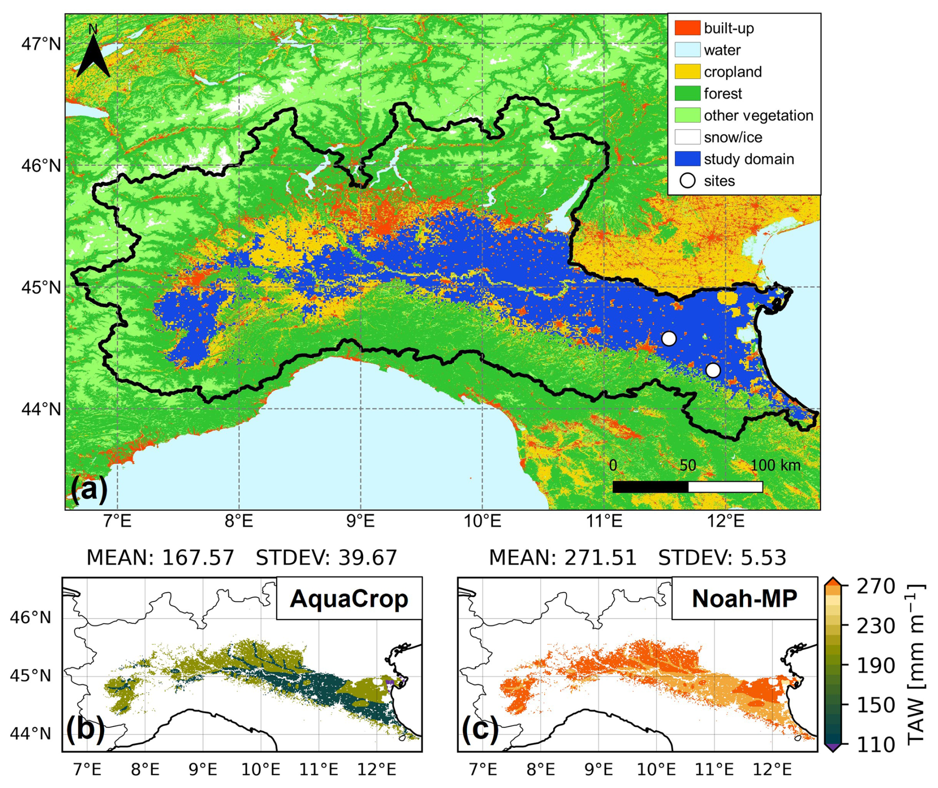
Figure 1 (a) Map of study domain showing a combination of the different CGLS land cover classes and the GRIPC irrigation classification. The rainfed cropland class and paddy rice are shown in yellow, different forest types are aggregated into one forest class in dark green, and the remaining vegetation classes are in light green. The dark blue areas correspond to irrigated cropland (excluding paddies) of interest to this study. The Budrio and Faenza sites are marked with white dots. (b, c) maps of the total available water (TAW) [mm m⁻¹] (for a root-zone depth of 1 m) derived from the soil hydraulic parameters of each model with Eq. (1), and for irrigated cropland only.

The specific area considered in this study consists of irrigated croplands at a 0.01° × 0.01° lat-lon spatial resolution. Cropland grid cells are derived from the 2019 Copernicus Global Land Service (CGLS) land cover map (Buchhorn et al., 2020), which is based on optical observations from the PROBA-V satellite. This land cover map was originally provided at a 100 m resolution. A 0.01° grid cell is defined as cropland if it is the dominant land cover class. Irrigated areas are derived from the Global Rain-fed, Irrigated and Paddy Croplands circa 2005 (GRIPC; Salmon et al., 2015) map. The original resolution of the GRIPC map is 500 m, in which the land is classified into (1) rainfed, (2) irrigated, and (3) paddies. A 0.01° grid cell is considered as fully irrigated if at least 50 % of the 500 m GRIPC grid cells within it are classified as “irrigated”. Grid cells that meet both conditions (cropland and irrigation) are represented by the dark blue color in Fig. 1a. Note that paddy areas (from the GRIPC map) are not included in this study; they are mainly present in the northwest part of the cropland patch, west and south of the large built-up area (Milan). Furthermore, clay soils were masked because AquaCrop only takes into account this specific texture class to simulate basin irrigation, specifically for paddy rice. For this purpose, AquaCrop clay soil parameters present a very low saturated hydraulic conductivity, and sprinkler irrigation would then lead to significant runoff losses that are unrealistic. These regions were found to be dominated by rice (https://sites.google.com/arpae.it/servizio-climatico-icolt/home?authuser=0, last access: 30 September 2024) with infiltration (or furrow) irrigation (Zucaro, 2014) and are mainly located in the eastern part of the Po Valley. A soil texture map of the region can be found in De Lannoy et al. (2024).

2.2 Models setups

2.2.1 General

The Noah-MP and AquaCrop model were run for 8 years covering the years 2015 through 2022 after spinup (10 years for Noah-MP, 5 years for AquaCrop given that the soil moisture for the latter model reaches field capacity every winter in the study region). Model output is produced for each day. AquaCrop runs at a daily resolution, whereas Noah-MP runs at a 15 min resolution but the output is averaged per day. Both models are run within NASA's LIS (Kumar et al., 2006, 2008) version 7.4, with the same texture and meteorological input. This subsection discusses the general settings common to both models. Table 1 shows the main differences. The model-specific settings and the definition of the growing season, defined as the period when irrigation is allowed, are presented in the next subsections.

(Raes et al., 2026)(Cosby et al., 1984; Chen and Dudhia, 2001)(Yang and Dickinson, 1996)

Table 1 Important model differences affecting irrigation. Note that the growing season is defined as the period when irrigation is allowed.

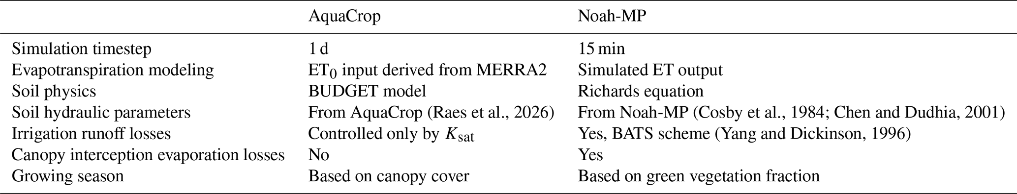
The models were forced with the Modern-Era Retrospective Analysis for Research and Applications, version 2 (MERRA2; Gelaro et al., 2017), originally provided at a spatial resolution of 0.5° latitude by 0.625° longitude. The forcing data were horizontally interpolated to the model grid using bilinear interpolation. Approximately 15 % of the study domain shows elevation differences larger than 200 m relative to the forcing grid, for which vertical downscaling (lapse-rate correction) may be beneficial. However, this correction was not compatible with AquaCrop v7.0 in NASA's LIS and was therefore applied only for Noah-MP. The temporal resolution of the data is hourly. AquaCrop requires the daily ET₀ as input, which is derived from the MERRA2 forcings using the Penman-Monteith equation (Allen et al., 1998) as in de Roos et al. (2021).

The soil texture classes were assumed to be homogeneous for the whole profile, identical for both models, and derived from the Harmonized Soil World Database (HWSD) v1.21. However, each model uses its own lookup tables to map the mineral soil texture to different estimates of associated soil hydraulic parameters (SHP), i.e. the water content at saturation θ_sat, at field capacity θ_FC, at wilting point θ_WP, and the saturated hydraulic conductivity, K_sat. Unlike other studies that improved the soil hydraulic parametrization for bucket-type models (e.g. Romano et al., 2011, 2025), in this study, the prescribed SHPs are used for each soil texture class without considering spatial variation, as is commonly done for large-scale simulations (De Lannoy et al., 2014; Kishné et al., 2017). Furthermore, soil organic carbon is not explicitly accounted for. For AquaCrop, indicative values of the SHPs are provided for each soil texture class (Raes et al., 2026), which are inherited from field-based applications (higher θ_WP and lower θ_FC), whereas Noah-MP has been developed and calibrated with different θ_FC and θ_WP values, defined by Chen and Dudhia (2001). More specifically, the Noah-MP SHPs are based on Cosby et al. (1984) and further adapted to intentionally increase total available water (TAW; also referred to as plant-available water) in the context of large-scale simulations by Chen and Dudhia (2001). Because of the inherent characteristics of the models, each model requires its own parameter set, which is further discussed in Sect. 4.2. No groundwater table, i.e. free drainage, was considered for both models, because the surface soil layers are generally disconnected from the deeper groundwater in the Po Valley, especially in the summer and over non-clay soils (excluded from this study).

Because each texture class has associated fixed θ_WP and θ_FC parameters, each soil texture class also has an associated TAW value, which varies dynamically with the active root zone and is calculated as follows:

$$\begin{array}{}\text{(1)}& \text{TAW}=\mathrm{1000}\cdot ({\mathit{\theta }}_{\mathrm{FC}}-{\mathit{\theta }}_{\mathrm{WP}})\cdot \text{RZ}\end{array}$$

where RZ is the root-zone depth [m], which is dynamic in both AquaCrop and Noah-MP (see next sections for more details). Figure 1b and c show the TAW over the domain for each model (i.e. set of SHPs) and is expressed for 1 m of rooting depth (RZ=1 m), to show the differences between the models. Across the different soil classes present in the domain, the TAW ranges are 80–200 and 255–276 mm m⁻¹ for AquaCrop and Noah-MP, respectively. In both models, the TAW is a key parameter for the irrigation modeling, as it is used to determine: (1) when irrigation should be applied, and (2) the amount of water required, as it is assumed that an irrigation application fills the root zone to field capacity. More specifically, irrigation is triggered based on the moisture availability MA [–], defined as the root-zone soil moisture content relative to the TAW:

$$\begin{array}{}\text{(2)}& \text{MA}={\displaystyle \frac{\mathrm{1000}\cdot (\mathit{\theta }-{\mathit{\theta }}_{\mathrm{WP}})\cdot \text{RZ}}{\text{TAW}}}\end{array}$$

where θ [m³ m⁻³] is the actual root-zone water content. The irrigation application is computed when the MA falls below a threshold (MA_irr) of 0.45, following Modanesi et al. (2022) who found that this threshold was optimal to follow the irrigation dynamics over the Budrio and Faenza fields (see Sect. 2.3.4) using Noah-MP. When the MA_irr threshold is reached, the irrigation amount applied corresponds to the water required to fill the root zone to field capacity. In the region, rooting depth varies with both soil conditions and crop type and typically ranges from 50 to 150 cm, with deeper root zones occurring near the edges of the Po River (Rivieccio et al., 2020). Therefore, the maximal root-zone depth was set to 1 m in both models but the actual rooting depth varies with the dynamic vegetation and therefore depends on the model. The period during which irrigation can be triggered (growing season) is explained in Sect. 2.2.4.

2.2.2 AquaCrop

AquaCrop v7.0 (Raes et al., 2009; Steduto et al., 2009) within LIS was used for the simulations of this study. The official FAO source code is open source for version 7 and higher (https://github.com/KUL-RSDA/AquaCrop/, last access: 29 April 2026).

In the context of a coarse-scale resolution study, it is common to use a spatially homogeneous generic crop type aiming at representing a biomass evolution that follows realistic dynamics within one grid cell (Mirschel et al., 2004; de Roos et al., 2021; Ingwersen et al., 2018), instead of specific crop types, which are more appropriate for high-resolution (field-level) studies. Therefore, the vegetation is parameterized as in de Roos et al. (2021), with a C₃ generic crop transplanted each year on 1 January and grown until the start of senescence in late August. Crop growth is limited by temperature and only occurs when temperatures exceed the base temperature of the generic C₃ crop, set to 8 °C. Spatial simulations with the generic crop were found to perform reasonably well when comparing soil moisture and biomass estimates with remote sensing products and in situ data (Busschaert et al., 2022; de Roos et al., 2021). Because the focus of this study is on irrigated areas, the choice was made to define a near-optimal soil fertility (similarly to Busschaert et al., 2022) since it is assumed that irrigated fields are well managed. Fertility stress is established to allow 80 % of the achievable biomass. The yearly CO₂ concentrations from the Mauna Loa station (Hawaii, US) are used.

For soil moisture, AquaCrop relies on the computation of an empirical water balance model (BUDGET; Raes, 2002), written as follows:

$$\begin{array}{}\text{(3)}& \mathrm{\Delta }S=P+\text{Irr}-E_{\mathrm{soil}}-\text{Tr}-\text{RO}-\text{Dr}\end{array}$$

where all flux components are water volumes per area, expressed in mm per time step of 1 d [mm d⁻¹]. ΔS is the change in soil water storage over the time step. Precipitation (P) and irrigation (Irr) are the incoming fluxes. The soil evaporation (E_soil), the transpiration (Tr), the surface runoff (RO), and the drainage (Dr) are the outgoing fluxes. The soil layer is divided into 12 compartments of equal size (0.1 m) to reach the total profile depth of 1.2 m (de Roos et al., 2021, 2024). The water balance is computed over the entire soil profile (12 compartments) and the change in storage ΔS for a certain time period is expressed as follows:

$$\begin{array}{}\text{(4)}& \mathrm{\Delta }S=\sum _{i=\mathrm{1}}^n\mathrm{\Delta }{\mathit{\theta }}_i\cdot D_i\cdot \mathrm{1000}\end{array}$$

with n, the number of compartments (12), θ_i [m³ m⁻³], the water content in compartment i, and D_i [m], the corresponding depth of the compartment. The sum of E_soil and Tr in Eq. (3) forms the actual ET. The computation of ET relies on the FAO approach and is described in Appendix A1. AquaCrop does not consider canopy evaporation (or leaf interception loss) explicitly, but it is indirectly included because the intercepted water is assumed to infiltrate into the surface soil, from where it can be lost by evaporation. RO consists of the water that does not infiltrate the soil and depends on a curve number and the K_sat. However, the infiltration of irrigation water is only limited by K_sat and not by the CN, since it is assumed that irrigation is well managed in AquaCrop. Since K_sat generally only limits the infiltration over clay soils, and pixels with clay soils are not included in this study (see Sect. 2.1), there will be no RO loss following irrigation. Finally, Dr (or deep percolation losses) occurs when the soil water content exceeds θ_FC.

In line with the Noah-MP configuration, the irrigation threshold is set to 45 % of the TAW. In AquaCrop, the irrigation threshold is defined in terms of depletion of the root-zone readily available water (RAW), which is itself a fraction of TAW determined by the crop-specific p-factor. For the generic C₃ crop used in this study, the p-factor is set to the default value 0.5, resulting in a depletion threshold of 110 % of RAW and allowing for limited water stress prior to irrigation. This configuration ensures conceptual consistency between the two modeling frameworks rather than optimization for a specific crop. The irrigation application depth (irrigation amount per event; Irr_appl in [mm d⁻¹]) can be written as follows:

$$\begin{array}{}\text{(5)}& {\mathrm{Irr}}_{\mathrm{appl}}=\mathrm{1000}\cdot ({\mathit{\theta }}_{\mathrm{FC}}-\mathit{\theta })\cdot \text{RZ}\left[{\mathrm{d}}^{-\mathrm{1}}\right]\end{array}$$

with θ [m³ m⁻³] being the root-zone water content before irrigation, already including the precipitation and potential ET of that day. The root-zone depth RZ [m] is defined by the crop parameters and starts at 0.1 m on 1 January to reach its maximum value (RZ_max) of 1 m after 80 calendar days.

2.2.3 Noah-MP

Noah-MP v4.0.1 (Niu et al., 2011) coupled to NASA LIS was run with the default LIS recommended parameters, as described in the LIS user manual except for the radiation transfer scheme and the dynamic vegetation option to allow for a dynamic green vegetation fraction (GVF [–]). The latter enables a dynamic definition of the growing season in line with AquaCrop (see Sect. 2.2.4). In contrast to AquaCrop, Noah-MP does not prescribe a sowing/planting date; vegetation growth and LAI evolve dynamically from carbon assimilation, with the growing season starting when environmental conditions allow net carbon gain (Niu et al., 2011). The radiation transfer had to be changed accordingly to make it compatible with the dynamic vegetation option. Note that these options were used in irrigation modeling studies using Noah-MP v3.6 in LIS (Modanesi et al., 2022). The vegetation parameterization is spatially homogeneous over the study domain, since only one land cover class (croplands) is considered. The main Noah-MP options used in this study are shown in Appendix B.

Noah-MP solves the energy and water balances. Similarly to AquaCrop (Eq. 3), the water balance for Noah-MP can be written as follows:

$$\begin{array}{}\text{(6)}& \mathrm{\Delta }S=P+\text{Irr}-E_{\mathrm{soil}}-E_{\mathrm{canop}}-\text{Tr}-\text{RO}-\text{Dr}\end{array}$$

In contrast to AquaCrop, Noah-MP estimates the ET fluxes based on the energy and water balances (Appendix A2), also considering the canopy evaporation (E_canop). Noah-MP solves the Richards' equations to compute vertical soil moisture distribution at a user-defined time interval (typically less than 1 h, here chosen at 15 min) and in 4 soil layers. The depths of the layers are 0.1, 0.4, 0.6, and 1 m, from top to bottom. Only the top 1 m is considered for the computation of the Tr. Note that water can also be stored in snow, but this is not considered in the ΔS of this study, since irrigation periods can be assumed to be snow-free.

To simulate irrigation, Noah-MP is coupled to an irrigation module developed by Ozdogan et al. (2010). When the MA_irr threshold is reached, the Irr_appl (Eq. 5) is calculated at 06:00 a.m. (local time), but the rainfall and potential ET of the rest of that day are not yet considered in the estimation of the root-zone water content θ before irrigation. RZ in Noah-MP is defined by the GVF:

$$\begin{array}{}\text{(7)}& \text{RZ}={\text{RZ}}_{\max }\cdot \text{GVF}\end{array}$$

with RZ_max, the maximum rooting depth [m] set to 1 m. The GVF is dynamically modeled from the leaf area index (LAI, m² m⁻²) with the following equation:

$$\begin{array}{}\text{(8)}& \text{GVF}=\mathrm{1}-e^{-\mathrm{0.52}\cdot \mathrm{LAI}}\end{array}$$

The Irr_appl is computed as in Eq. (5) and is equally distributed at each model time step (15 min) and applied from 06:00 to 10:00 a.m. (local time) and added to the precipitation.

2.2.4 Growing season

For both model setups, a dynamic start of the growing season (time window when irrigation is allowed) was defined. In Noah-MP, the growing season was initially described by Ozdogan et al. (2010) as the period where the GVF is larger than 40 % of the range between the minimum and maximum GVF (GVF_min and GVF_max). This definition has been used in several studies (Lawston et al., 2017; Lawston-Parker et al., 2023; Modanesi et al., 2021b; Sharma et al., 2022). GVF_min and GVF_max were defined based on a deterministic run with irrigation by taking the average minimum and maximum GVF over the 8 years. In AquaCrop, the fraction of land covered by vegetation, the canopy cover (CC), is used to simulate the crop development, with the minimum CC (or initial CC) equal to 0.1 [–] and a maximum CC of 0.85, both being crop parameters (developed by de Roos et al., 2021). By definition, the CC should correspond to the GVF in Noah-MP. The threshold for the growing season for both models can then be summarized as follows:

$$\begin{array}{}\text{(9)}& {\mathrm{veg}}_{\mathrm{irr}}={\mathrm{veg}}_{\min }+\mathrm{0.4}\cdot ({\mathrm{veg}}_{\max }-{\mathrm{veg}}_{\min })\end{array}$$

where veg [–] corresponds to the GVF and CC for Noah-MP and AquaCrop, respectively. In Noah-MP, GVF is diagnostically derived from the prognostic LAI through an exponential relationship (Eq. 8), whereas in AquaCrop, the CC is the primary state variable driving surface fluxes and is explicitly controlled by crop growth parameters and stress responses.

2.3 Evaluation

To evaluate the simulations, satellite products of soil moisture, vegetation, and ET are used, along with field-level (in situ) irrigation data. Note that all these reference products have their uncertainties, in particular over irrigated areas (see Sect. 4). The usage of coarse-scale satellite retrievals is considered to complement the in situ (field-level) evaluation, as the latter might lead to representativeness errors when used to evaluate coarser-scale simulations. Due to constraints in the temporal frequency of validation products and inevitable mismatches between the modeled timing of irrigation and the human decision to irrigate, the evaluation is performed on temporally aggregated values.

2.3.1 Soil moisture

The surface soil moisture (SSM) model estimates were evaluated against downscaled SSM from the Soil Moisture Active Passive (SMAP) mission, referred to as the NASA SMAP 1 km product (Fang et al., 2022). These SMAP SSM retrievals were downscaled using thermal and optical data and should therefore be able to detect the presence of irrigation, as proven for similar downscaled products (Merlin et al., 2013). The data perform better in low and mid-latitudes and during warm months (Fang et al., 2022). The product sometimes fails to capture localized events, although this limitation a shared concern for all downscaled products (Brocca et al., 2024). The SMAP 1 km product is provided on an EASEv2 grid and was reprojected to the model grid with a nearest neighbor function. Both descending (06:00 a.m.) and ascending (06:00 p.m.) observations were considered, and when both were available on the same day, the arithmetic mean was taken. The first soil layer moisture from both models was used for the evaluation, representing the top 10 cm of the soil. To reduce the impact of short-term errors in the irrigation timing, the SSM estimates were averaged over 15 d for the evaluation without first cross-masking the data. The SSM is evaluated for the months from March through September, as AquaCrop simulates an annual crop with senescence in September, and presents no vegetation thereafter. The SSM evaluation time ranges from 1 April 2015 (start of available SMAP observations) through 29 September 2022.

2.3.2 Vegetation

To evaluate the vegetation estimates of both models, the Copernicus Global Land Service (CGLS) Dry Matter Productivity (DMP) was used (Buchhorn et al., 2020). The product offers DMP 10-daily average DMP observations retrieved with PROBA-V (before August 2020) and Sentinel-3 (from August 2020) using the fraction of absorbed photosynthetically active radiation (fAPAR; Monteith, 1972; Penman, 2003). These retrievals are known to not capture the short-term water stresses accurately. However, since this study only concerns irrigated areas, water stress should remain limited compared to rainfed areas. The units of the DMP are kg ha⁻¹ d⁻¹, averaged over 10 d. The data were resampled from a 300 m resolution to the model grid via averaging. The DMP was used to evaluate the 10 d averaged daily biomass production from AquaCrop, derived from the cumulative biomass, and the net primary production (NPP) from Noah-MP. The daily biomass production from AquaCrop is directly comparable to the DMP, whereas the NPP (expressed in g C m⁻² d⁻¹) was converted to DMP by multiplying the value by 2 since in the derivation of the DMP product, it is assumed that the dry matter is composed of 50 % of carbon (Swinnen et al., 2019). Similarly to the SSM, the vegetation was evaluated for the months March through September, and also separately for the first half of the year (January–June) corresponding to the period when the AquaCrop CC increases (before reaching a plateau in the summer) as in de Roos et al. (2024).

2.3.3 Evapotranspiration

The ET was evaluated using the SenET product that provides daily estimates at a 100 m spatial resolution from 2017 through 2021 (Bartkowiak et al., 2023). The ET is derived using the two-sourced Energy Balance model that downscales the original 1 km Sentinel-3 land surface temperature using Sentinel-2 surface reflectances. For consistency with the model grid, the data were reprojected by spatial averaging. As a result, the ET estimates remain primarily constrained by the original 1 km Sentinel-3 land surface temperature; however, the re-aggregation may introduce some uncertainty. Differences in spatial and temporal resolution among ET products can influence evaluation results. Nevertheless, substantial inconsistencies among existing ET products have been documented in previous studies (De Lannoy et al., 2024; Modanesi et al., 2025), and no definitive reference dataset for ET currently exists. SenET was therefore selected for its potential suitability for irrigation management applications (Bartkowiak et al., 2024; Chintala et al., 2022; Spiliotopoulos et al., 2023). Similarly to the SSM evaluation, the ET evaluation is performed for the months March through September, on 15 d averages (expressed in mm d⁻¹) to reduce the impact of short-term errors in irrigation timing.

2.3.4 Irrigation

Over the entire Po Valley, the average irrigation water use reported by water management agencies is around 500–600 mm yr⁻¹ computed for varying irrigated areas (https://suwanu-europe.eu/wp-content/uploads/2021/05/State-of-play_Po-River-Basin-Italy.pdf, last access: 3 February 2026). Field-based irrigation data is available for three sites and was collected for the ESA IRRIGATION+ project by the Canale Emiliano Romagnolo (CER) consortium, and has been used as benchmark in several studies (Dari et al., 2023; Modanesi et al., 2021a, 2022; Le Page et al., 2023). The Budrio fields consist of five experimental plots within one LIS pixel, covering three irrigation seasons from 2015 through 2017 (top white dot in Fig. 1), with the most common crops being tomatoes and maize using drip and sprinkler irrigation. The daily irrigation rates (in mm d⁻¹) were spatially averaged to compare with the irrigation estimates from the models. The Faenza fields (bottom white dot in Fig. 1) are separated into two districts: Faenza San Silvestro (2.9 km², covering 3 LIS pixels), and Faenza Formellino (7.6 km², 8 pixels). These in situ irrigation rates cover 2016 through 2021 with pear and kiwi as dominant crops using mainly drip irrigation. In this case, the LIS output of multiple pixels was averaged for the fields in each district. Irrigation is evaluated for the months of March through September and is temporally averaged from weekly to seasonal time intervals.

2.3.5 Metrics

The SSM, vegetation, and ET are evaluated in terms of Pearson correlation (R), bias, root mean square difference (RMSD), and unbiased RMSD (ubRMSD), with independent satellite data. Irrigation is evaluated in terms of R, bias, and RMSD with in situ reference data. The metrics are calculated as follows:

$$\begin{array}{}\text{(10)}& {\displaystyle }R={\displaystyle \frac{{\sum }_{n=\mathrm{1}}^N(x_n-\overline{x})(y_n-\overline{y})}{\sqrt{{\sum }_{n=\mathrm{1}}^N(x_n-\overline{x}{)}^{\mathrm{2}}{\sum }_{n=\mathrm{1}}^N(y_n-\overline{y}{)}^{\mathrm{2}}}}}\text{(11)}& {\displaystyle }\mathrm{bias}={\displaystyle \frac{{\sum }_{n=\mathrm{1}}^N(x_n-y_n)}{n}}\text{(12)}& {\displaystyle }\mathrm{RMSD}=\sqrt{{\displaystyle \frac{\mathrm{1}}{N}}\sum _{n=\mathrm{1}}^N(x_n-y_n{)}^{\mathrm{2}}}\text{(13)}& {\displaystyle }\mathrm{ubRMSD}=\sqrt{{\text{RMSD}}^{\mathrm{2}}-{\text{bias}}^{\mathrm{2}}}\end{array}$$

where x is the value of the simulated land surface variable from AquaCrop or Noah-MP, y is the reference value (observation), and N is the number of reference data in time ($n=\mathrm{1},\mathrm{\dots },N$). $\overline{x}$ and $\overline{y}$ represent the temporal mean values. By definition, the bias scales linearly with temporal aggregation (for irrigation, SSM, ET) and can therefore be consistently related across aggregation levels. In addition to these metrics, the Pearson R of the anomalies (anomR) is calculated since the evaluated variables present strong seasonal patterns. The anomalies are calculated by subtracting the long-term climatology from the observations. A window size of 30 d was taken to calculate the climatology.

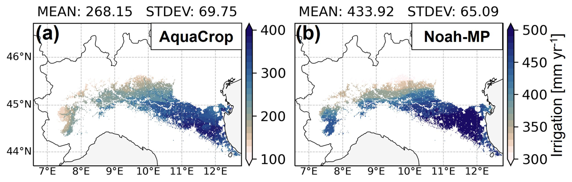
Figure 2 Average irrigation [mm yr⁻¹] over the 8 years for (a) AquaCrop and (b) Noah-MP. Note the different ranges in colorbars.

3 Results and discussion

3.1 Basin-scale evaluation

3.1.1 Irrigation estimates

The multi-year average annual irrigation rates estimated by both models are presented in Fig. 2. Irrigation amounts are larger for Noah-MP (434 mm yr⁻¹) than for AquaCrop (268 mm yr⁻¹). This contrast can be explained by differences in irrigation losses (not consumed by transpiration), growing season lengths (shown in Appendix C), and calculation procedures between the models, and is later discussed in Sect. 3.1.3.

The spatial patterns in irrigation rates are similar in both models, presenting a strong north-south gradient. The main drivers for both models are radiation and precipitation, presenting similar spatial patterns (not shown here but detailed in De Lannoy et al., 2024). The irrigation pattern can also be linked to the average growing season length (Fig. C1). The upper southwestern region shows strong differences in average irrigation rates between AquaCrop and Noah-MP. In the latter, there is more vegetation and the growing season covers almost the entire year, whereas it is much shorter for AquaCrop (Appendix C) and the increase in CC occurs later in the season.

Management information of the Po Valley indicates that average irrigation rates are around 500 to 600 mm yr⁻¹ which is more than what is estimated by either AquaCrop or Noah-MP. This might be because in reality irrigation water is lost (not taken up by vegetation) in various ways that the models do not, or only in a limited way, account for. AquaCrop aims to estimate a net irrigation amount and only accounts for soil evaporation losses. Noah-MP additionally simulates canopy interception and surface runoff losses, which can occur for sprinkler irrigation. However, neither of the models explicitly represents percolation losses due to irrigation, which can be substantial for surface irrigation systems (dominant irrigation method over the area). Surface irrigation (channel-type) is relatively the most inefficient irrigation system (Irmak et al., 2011) in terms of application losses, but also in terms of conveyance losses, as water is distributed through open canals. Adding a typical conveyance efficiency factor for the area (0.825; Rohwer et al., 2007) to the Noah-MP estimates would yield an average value of 526 mm yr⁻¹ which is consistent with management data.

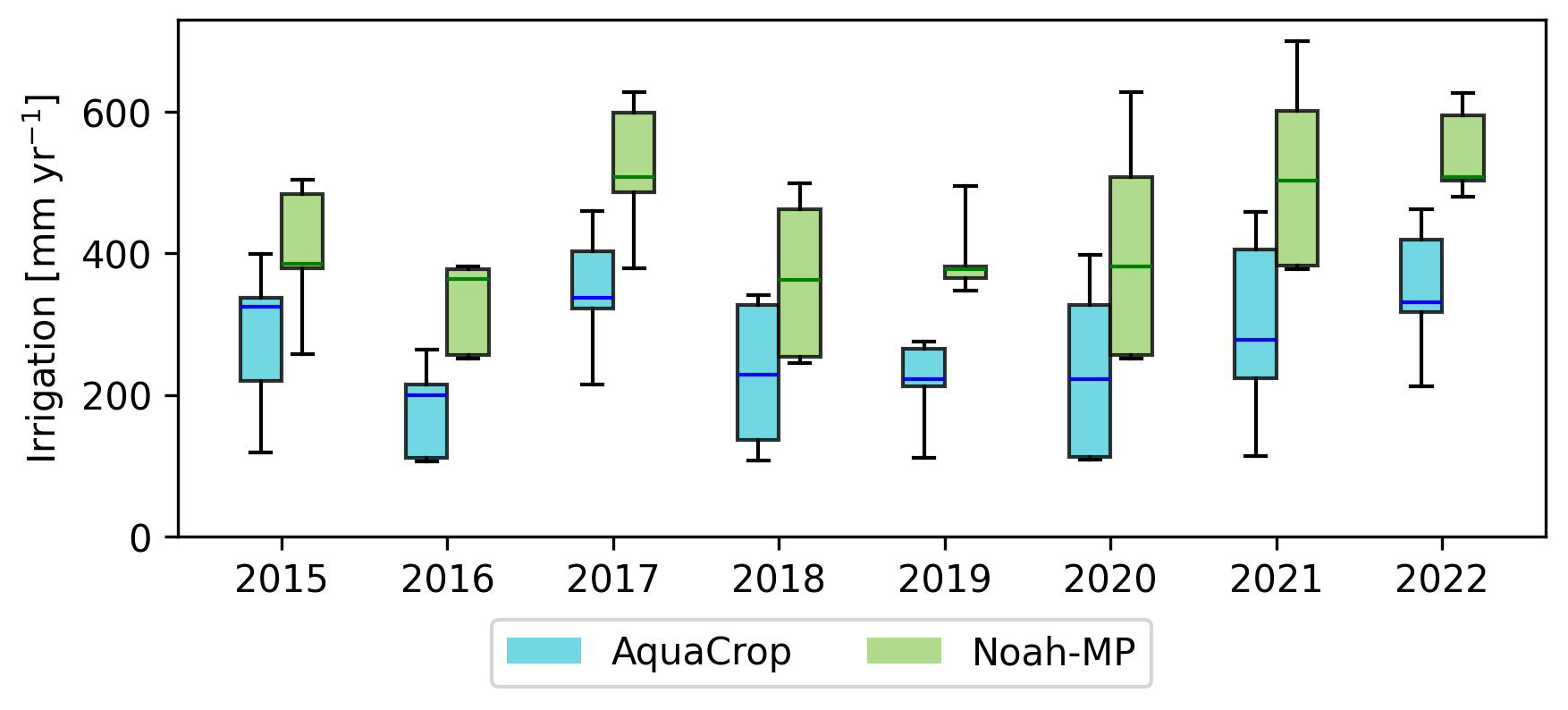
Figure 3 Yearly irrigation amounts [mm yr⁻¹] for 2015 through 2022 for AquaCrop (blue) and Noah-MP (green). The boxes represent the irrigation values within the interquartile range (IQR), the lines in the boxes correspond to the median, and the whiskers extend to Q1 − 1.5 ⋅ IQR and Q3 + 1.5 ⋅ IQR or are cut off if all data points are within the interval (outliers are not shown).

Figure 3 presents spatial boxplots of the annual irrigation rates for both models. More specifically, the interannual variability of the irrigation estimates is shown following the x-axis, and the spatial variability over the domain is represented by the extent of the boxes. First, as expected given the shared meteorological forcing, the temporal evolution of median irrigation is similar in both models, with Noah-MP consistently producing higher irrigation amounts, in line with the average annual irrigation rates shown in Fig. 2. Second, the spatial variability also follows the same trends for both models, with a reduced variability in 2019 due to less variation in summer precipitation and temperatures over the domain. On average, 2017 and 2022 appear to be the years with the most intensive irrigation, followed by 2021, all years being very dry (Baronetti et al., 2020; Montanari et al., 2023). The results presented in our study are mainly driven by the meteorological forcings and have no limitation in irrigation water usage, while in reality, farmers likely irrigate according to a schedule and not depending on moisture deficit thresholds (Pokhrel et al., 2016), and may also face water-use restrictions during drought years.

3.1.2 Soil moisture, vegetation and ET

Figure 4 presents the evaluation of the SSM, vegetation, and ET estimates from the models with downscaled SMAP 1 km SSM, CGLS DMP, and SenET, respectively. Both observed and simulated SSM and ET are aggregated over 15 d to limit the negative impact of erroneous timing of irrigation events. The daily biomass production of AquaCrop, and the NPP of Noah-MP are averaged over 10 d to be compared to the 10-daily DMP product. For all variables, the months March through September are considered, and for DMP, an additional evaluation is provided for the months January through June, corresponding to the period when the AquaCrop canopy cover increases (before reaching a plateau in summer).

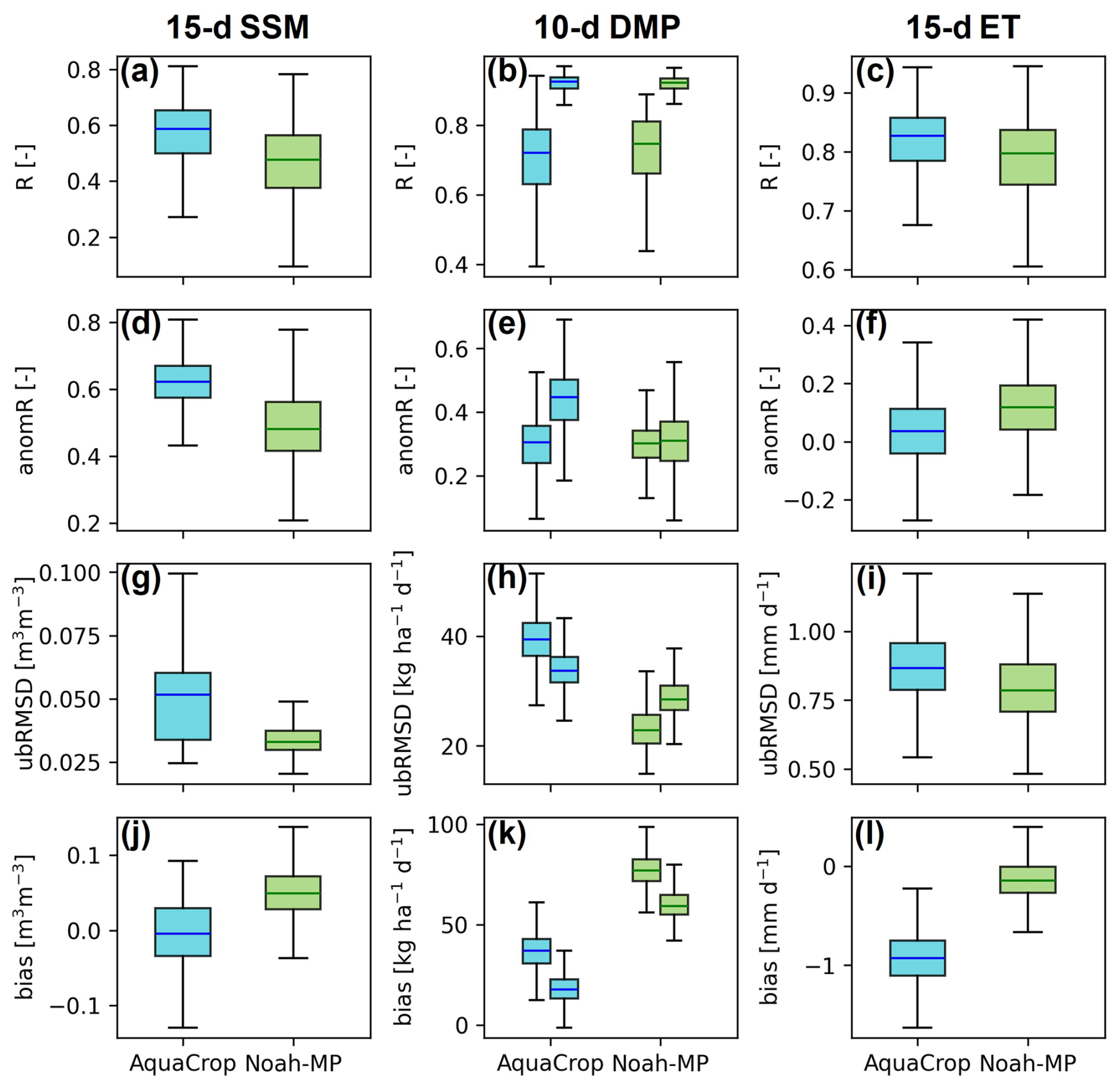
Figure 4 Boxplots of R, ubRMSD, anomR, and bias of AquaCrop (blue) and Noah-MP (green) simulations, comparing (i) modeled SSM with SMAP SSM, (ii) modeled vegetation with CGLS DMP, (iii) modeled ET with SenET. Metrics were computed for the months March through September 2015–2022 for SSM and vegetation, and the same months but 2017–2021 for SenET. For the evaluation with CGLS DMP, the second boxplot presents the metrics computed for the months from January through June 2015–2022.

For the evaluation with SMAP SSM, AquaCrop on average shows a higher (anom)R than Noah-MP. However, the error (ubRMSD) is significantly higher for AquaCrop, because AquaCrop SSM tends to hit the lower and upper boundaries (θ_WP and θ_FC) more frequently. Several areas perform poorly in terms of ubRMSD and R for both models (metric maps shown in Appendix D). These areas correspond to the surroundings of the large cropland area that is classified as paddy in the GRIPC map of Salmon et al. (2015) and which was masked in this study. According to the CORINE land cover map (Büttner, 2014) of 2018, these low-performance regions (the triangle at the confluence of the Ticino and Po rivers, and southern Milan) are classified as rice fields also under flood irrigation (Zucaro, 2014). The irrigation practices applied in rice fields differ strongly from the sprinkler-type irrigation assumed in AquaCrop and Noah-MP, as basin irrigation with prolonged ponding deviates even more strongly from these assumptions than other surface irrigation methods. In addition, the downscaled SMAP retrievals may be uncertain over these complex areas.

For the vegetation evaluation, Noah-MP shows better skill than AquaCrop in terms of R and ubRMSD during the main growing season (March through September). Compared to this time period, AquaCrop performs significantly better during the first part of the year (January through June), where variations in DMP are mainly driven by low temperatures (below the baseline temperature defined at 8 °C for the generic crop, causing cold stress). Later in the season, when temperatures are higher, the biomass production is only limited by water stress, which only slightly affects the transpiration when the root-zone soil moisture becomes less than 50 % of TAW (close to the irrigation threshold set at 45 % of TAW). Both Noah-MP and AquaCrop vegetation estimates are highly positively biased compared to the CGLS DMP. For AquaCrop, a biomass overestimation could be due to uncalibrated crop parameters, e.g. the maximum canopy cover (CC_max) which is a determining factor for biomass production. A second influential factor could be the fertility stress, here chosen to be near optimal (80 % of the potential biomass is produced), which may be an overestimation for the Po Valley. Previous studies have also shown strong vegetation overestimations by Noah-MP in terms of GPP, particularly over croplands (De Lannoy et al., 2024; Ma et al., 2017). Especially for irrigated land, the growing season is extended, and again, harvest is not modeled. The choice of vegetation module options in this study may have resulted in even stronger overestimations as those may not be the most optimal ones for the area (Li et al., 2022). Time series of SSM and DMP are presented and discussed in Sect. 3.2.

The ET evaluation against the SenET product generally shows a better agreement with the Noah-MP estimates, as shown by the higher anomR and lower ubRMSD. This result can be expected, as Noah-MP solves an energy balance to compute the ET, whereas a reference ET estimate (ET₀) is required as input for AquaCrop. The latter model then converts the ET₀ to the actual ET by using a crop coefficient (K_c), proportional to the CC, and a stress factor (K_s) considering heat and water stresses. More details on the ET computation for both models can be found in Appendix A. Note that AquaCrop ET estimates present an important negative bias (underestimation) compared to SenET. This bias is typically larger in spring because vegetation tends to develop later for AquaCrop. Therefore, the bias is even more severe in the colder regions, where the crop develops even later (as shown by the growing season maps in Fig. C1). The spatial patterns of the metrics are similar for both models (Appendix F), with lower anomR values in the eastern part of the domain which is likely dominated by infiltration irrigation (Zucaro, 2014). Appendix G shows time series of ET estimates from both models and SenET for the three test sites.

For all three satellite retrievals, it is important to note that, in addition to potential retrieval biases, the 0.01° spatial resolution implies that each pixel represents a mixture of land covers and crop types. This sub-pixel heterogeneity can contribute to apparent inconsistencies in the evaluation. In particular, the resampled DMP and ET may include signals from non-cropland vegetation, whereas both models simulate only croplands, potentially leading to a bias. In addition, mismatches in crop phenology may play a role. The generic summer crop used in AquaCrop differs from cropping systems that include winter crops such as wheat, for which ET typically increases earlier in the season. These differences in land cover composition and phenological timing can therefore partly explain the contrasting biases observed in vegetation and ET.

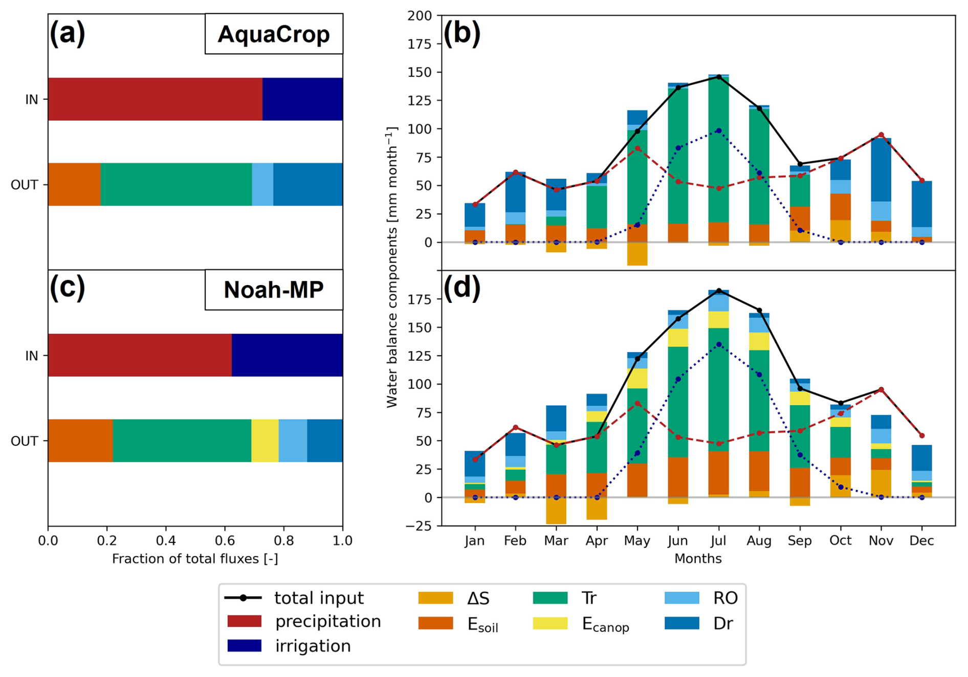
Figure 5 (a, c) Year-round water balance components averaged across all years and normalized by the sum of input and output fluxes for (top) AquaCrop and (bottom) Noah-MP. (b, d) Corresponding monthly water balance components. The precipitation and irrigation are represented by the dashed red lines and the dotted blue lines. ΔS is on average ∼0 mm in (a) and (c), whereas it can be either positive (increase in storage) or negative (decrease) in the monthly estimates of (b) and (d).

3.1.3 Water balance

To better understand the similarities and differences between the irrigation estimates simulated by both models, an overview of the different water balance components is presented in Fig. 5. The distribution of the fluxes (normalized by the total input or output flux) over the 8 years is shown in Fig. 5a and c, while Fig. 5b and d present the monthly climatology (average flux in mm per month over the 8 years). For the change in storage (ΔS) in Fig. 5b and d, only the top 1 m layer is considered to cover the modeled maximal rooting depth and because it is mainly the first meter of soil that shows large fluctuations over time. As shown in the water balance equation of AquaCrop (Eq. 3), canopy interception is not considered. Also, note that the output fluxes shown in Fig. 5b and d do not always add up to the total incoming fluxes (sum of precipitation and irrigation, black line) because the climatology may not be robust enough over 8 years and snow is not accounted for in ΔS (considered in Noah-MP but not in AquaCrop).

The results confirm the higher irrigation rates for Noah-MP presented in Fig. 2. The main factor explaining those differences is that the models differ considerably in the losses of the water inputs (precipitation and irrigation), namely via surface runoff and evaporation. Surface runoff, similar for both models during winter, is significantly higher for Noah-MP during summer, mainly due to irrigation applications. This is not the case for AquaCrop, because runoff generation due to infiltration excess (from irrigation) can only happen if the infiltration is limited by the soil K_sat, but this was not a limiting factor for the dominant soil textural classes of the study domain (sandy loam and silt loam). In Noah-MP, surface runoff during irrigation is generated through a runoff scheme (Yang and Dickinson, 1996), which is appropriate for representing infiltration-excess runoff from rainfall at the grid scale. However, when applied to large irrigation applications, as shown in Sect. 3.2, the resulting runoff losses are not compensated by additional irrigation input, preventing soil moisture from reaching field capacity and leading to an unrealistic representation of field-scale irrigation. In addition to surface runoff, the evaporative losses (E_soil and E_canop) in Noah-MP are larger compared to AquaCrop.

The length of the growing season also contributes to the difference in the average irrigation rates. Noah-MP vegetation develops earlier, leading to increased transpiration in spring compared to AquaCrop. The root zone depletes more rapidly (negative ΔS) and causes more irrigation (blue dotted line in Fig. 5b and d) for Noah-MP in the early season. The irrigation applications end in September for AquaCrop (due to the fixed onset of senescence) or October for Noah-MP. This induces some additional irrigation in the late season, which is not simulated by AquaCrop.

The models present differences in the ET estimates. In general, the proportion of ET, the i.e. sum of E_soil, Tr, (and E_canop for Noah-MP only), relative to the other fluxes is larger for Noah-MP than for AquaCrop (Fig. 5a and c). However, the absolute values of Tr are considerably higher for AquaCrop during the summer, even if less irrigation water is applied in AquaCrop, which is explained by lower E_soil, the absence of E_canop, and runoff losses after irrigation. No Tr is simulated by AquaCrop during the winter months because of the absence of vegetation. Tr increases earlier for Noah-MP at the beginning of the season, which can be explained by earlier and more vegetation for Noah-MP (also resulting in a better agreement with SenET, Fig. 4). This early increase in Tr leads to faster and earlier drying of the soil for Noah-MP, represented by the negative ΔS in Fig. 5b and d. Tr is also higher for Noah-MP than AquaCrop in the fall, because of vegetation senescence in late August and early September for AquaCrop. The soil water refill begins earlier compared to Noah-MP (shown by the positive ΔS in September). Lastly, the absolute values for ΔS also present smaller fluctuations for AquaCrop. The bottom layers of the soil profile in AquaCrop (deeper than 0.6 m) mostly remain close to θ_FC due to the soil water modeling scheme.

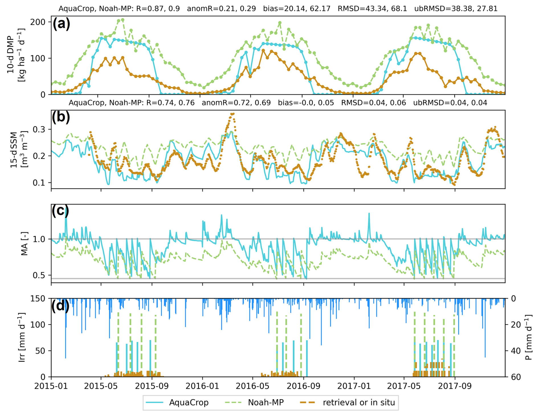
Figure 6 Times series of different variables for AquaCrop (full blue lines), Noah-MP (dashed green lines), and reference data (dashed ochre lines and points) at the Budrio site. (a) 10 d DMP [kg ha⁻¹ d⁻¹] of both models and CGLS DMP. (b) 15 d SSM [m³ m⁻³] from both models and SMAP. (c) moisture availability (MA [–]). (d) irrigation from both models and field data [mm d⁻¹] (left y axis) and precipitation [mm d⁻¹] from MERRA2 (right reverted y axis). For a and b, the metrics of both model estimates against the reference are shown in the title.

3.2 Field-based evaluation

A detailed analysis was performed over the Budrio (sandy loam) site and is presented in Fig. 6 for the years 2015–2017 (with 2017 being a very dry year), corresponding to the availability of the irrigation data on that site. The figure presents the (a) DMP, (b) SSM, (c) moisture availability (MA; Eq. 2), and (d) irrigation and rainfall (incoming fluxes). The summary metrics on top of Fig. 6a and b are computed on the entire three years presented in the time series (unlike Fig. 4, which focused on select months).

In line with the basin results, the biomass of both models follows the expected seasonal cycle. AquaCrop performs reasonably during the first months of the growing season, and then keeps a slight declining plateau as soon as the maximum CC is reached. In AquaCrop, crop growth can only be affected by (1) temperature stress (heat), and (2) water stress. The variations in DMP in the early season are due to temperature (cold stress), and some decreases in DMP are captured by AquaCrop (e.g. spring 2015). But as soon as the CC reaches its maximum value, temperatures are warm enough to avoid cold stress and since the crop is fully irrigated, the water stress is limited, explaining this plateau. As discussed above, Noah-MP estimates more vegetation over a longer growing season.

In terms of SSM estimates, AquaCrop generally shows a lower SSM compared to Noah-MP, especially in summer (during the irrigation period), due to the absence of the modeling of capillary upward water flow. Noah-MP SSM remains high in summer due to regular large irrigation applications, as also shown by Modanesi et al. (2021b). It is important to note that the soil parameters and soil water modeling assumptions are different (Table 1). AquaCrop SSM rapidly reaches its boundaries (θ_WP=0.10 and θ_FC=0.22 m³ m⁻³ for this site) while the 15 d SSM from Noah-MP keeps a smoother intermediate value, far from θ_WP (0.05 m³ m⁻³) and θ_FC (0.31 m³ m⁻³).

The differences in SHPs (θ_WP and θ_FC) represent one of the main factors causing the difference in irrigation application (irrigation amount per event, or per day). The TAW of a 1 m soil layer for Noah-MP is significantly larger than for AquaCrop (260 versus 120 mm) meaning that more water is required to bring the root zone back to θ_FC. For AquaCrop, once the maximum root-zone depth is reached (1 m) the irrigation application corresponds to 66 mm (with slight variations, as AquaCrop considers the losses through potential ET, and the gains in rainfall of that day). For Noah-MP, the MA is computed at 06:00 a.m. and if the threshold is reached, the exact amount of water required to bring the soil back to field capacity is computed, not considering any losses (potential ET or runoff) or gains (rainfall). Figure 6c shows the MA, but note that the daily averaged MA is presented for Noah-MP (and not at 06:00 a.m., time when the MA is evaluated in the model).

The benchmark irrigation data are shown along with the irrigation estimates in Fig. 6d. First, the in situ irrigation (ochre lines) starts earlier than predicted by the models. In reality, the start is dependent on the meteorological forcings (included in the modeling) but also on the crop type, and irrigation practice. For instance, water may be required during early development stages for certain crops, or farmers may apply pre-sowing irrigation, which are both factors not considered by the models in this study. Second, the in situ amounts are lower and more distributed since an average of five fields was considered (except for the last year 2017 when in situ irrigation data are only available for one field). Therefore, large model peaks are difficult to compare with these distributed amounts and temporally aggregated amounts may be more relevant.

Lastly, the total modeled annual irrigation stands out in 2017 (dry year), whereas the in situ data does not show an increase in irrigation for that year (both 2015 and 2017 show an annual irrigation of ∼350 mm). The satellite retrievals show a lower SSM and a lower DMP in the summer 2017 for the pixel, effectively suggesting a dry year that was perhaps not compensated in the field by irrigation due to water limitations.

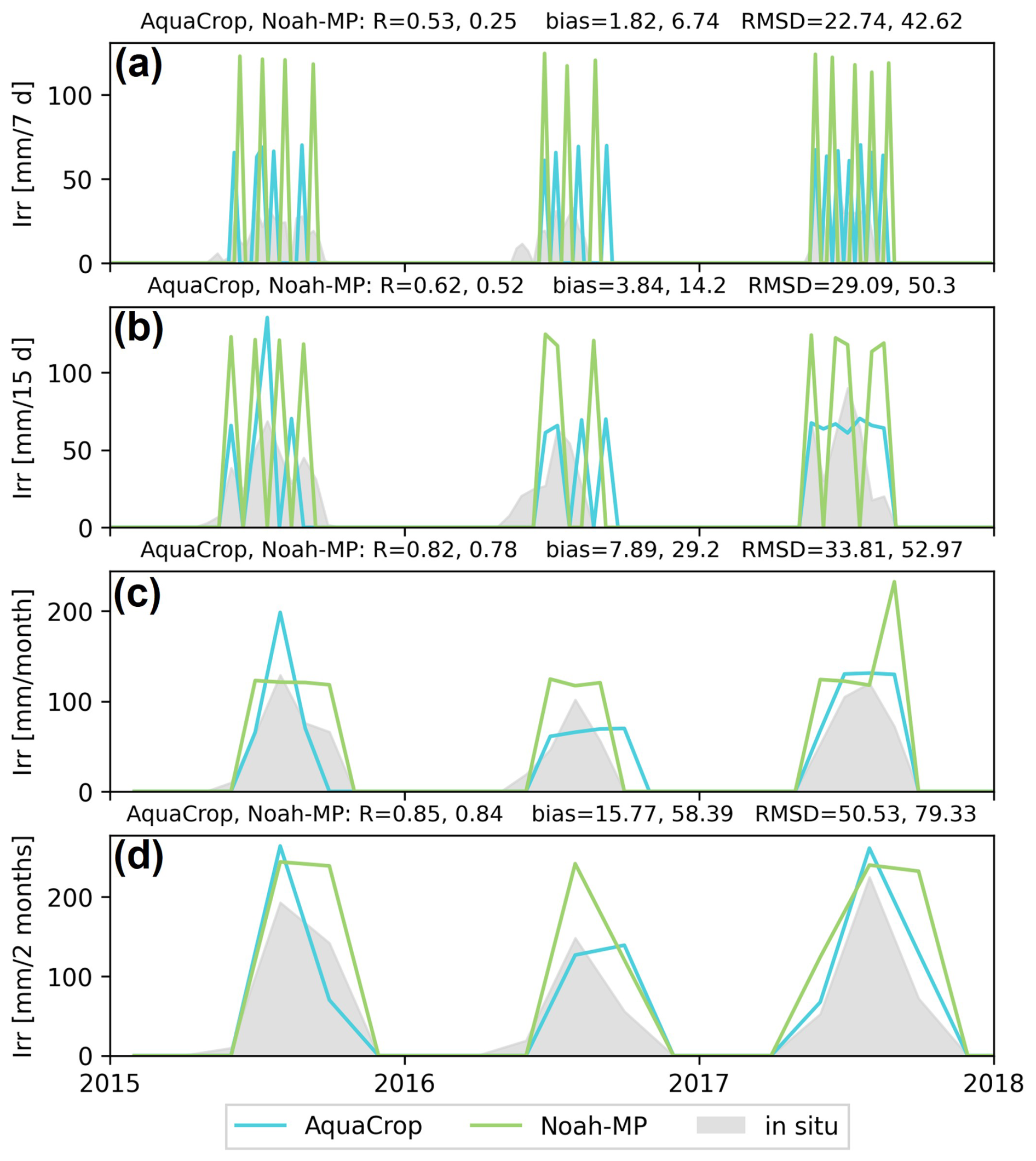
Figure 7 Irrigation time series for the Budrio site aggregated over different time intervals. The metrics are computed for the months March through September.

Figure 7 shows the in situ and estimated irrigation for different temporal aggregation levels (weekly, two-weekly, monthly, and two-monthly). The correlation metrics relative to in situ data increase steadily with longer aggregation windows. Both models tend to overestimate the irrigation against in situ data at this field, with the most positive bias for Noah-MP. On shorter aggregation intervals (7 and 15 d), AquaCrop agrees better with the in situ irrigation amounts since the irrigation application depths are much smaller and therefore more distributed. For longer aggregation intervals (one and two months), Noah-MP also shows a good performance by capturing the irrigation amounts but presents less interannual variability than AquaCrop. Less irrigation was applied in 2016, which is also simulated by AquaCrop but not clearly by Noah-MP.

The results over the Faenza sites in Appendix H confirm that simulated irrigation from both models correlate best with in situ data for longer aggregation intervals. The correlation is higher for AquaCrop for seasonal irrigation estimates, and the limited interannual variation is better captured by AquaCrop. However, both models show a strong irrigation overestimation, with sometimes more than double the amount observed. Overestimations were also found in other studies (Dari et al., 2023; Modanesi et al., 2022) and are likely due to the dominance of fruit trees (mainly kiwi) for these sites, typically supplied through localized methods (drip irrigation), which are more efficient than sprinkler irrigation.

4 Overview, limitations, and future perspectives

4.1 Overview of the modeling results

The results have shown that both a crop model, AquaCrop, and an LSM, Noah-MP can approximate the average large-scale irrigation rates, after identifying and accounting for the losses. By design, AquaCrop simulates net irrigation amounts and Noah-MP estimates irrigation amounts with minimal application losses, and both do not account for larger transportation and application losses that are included in the reported water records (on average 500–600 mm yr⁻¹). It is important to note that AquaCrop is computationally less expensive, especially because it runs at a daily time step (and not 15 min as chosen for Noah-MP, required to avoid instabilities in flux computations). Unsurprisingly, both models estimate very different amounts and timing of irrigation, and the temporal dynamics converge with temporal aggregation. With temporal aggregation, the modeled dynamics better match the in situ data at sparse sites. The evaluation of other land surface estimates (SSM, DMP, ET) showed a mixed performance for both models. While Noah-MP showed lower errors (ubRMSDs) for all three evaluated variables, AquaCrop sometimes showed a better performance in terms of (anom)R. However, the inconsistency between the limited available irrigation reference data (water managers, satellite proxies, field data) makes it difficult to perform a conclusive model evaluation. The current limitations in reference in situ and satellite-based datasets is discussed below in Sect. 4.3 and 4.4.

4.2 Model limitations, potential improvements, and future perspectives

Noah-MP was originally not designed to accurately model irrigation or even crop growth at the field scale. The key soil parameters θ_WP and θ_FC were defined to obtain accurate fluxes (ET), in a mosaic of different land covers (Chen and Dudhia, 2001). For the field-based application, the Noah-MP TAW of the different soil textural classes (Fig. 1b and c) is not in line with agricultural applications, leading to unrealistic irrigation events (>100 mm per application, Fig. 6). Additional simulations were performed (not shown) using the more realistic soil parameters for field-based applications as used in AquaCrop, but the results of the Noah-MP and AquaCrop models then diverged even further, with a drastic increase in ET for Noah-MP. This further underscores that each model is developed with its own set of parameters, highlighting that soil moisture is a model-dependent quantity (Koster et al., 2009), and that each model has its own coupling mechanisms between soil moisture and fluxes of ET, runoff (Crow et al., 2024) and irrigation. Therefore, rather than harmonizing these parameters, we retained the native model parameterization and interpreted the results within a process-oriented intercomparison framework, rather than a direct comparison with harmonized parameter settings. However, for longer aggregation intervals (monthly to annual), the exact values of each SHP are of secondary importance, as the difference in process representation between the models is the primary explanation for the difference in irrigation estimation. The Noah-MP vegetation estimates were largely biased compared to the CGLS DMP data, in line with Li et al. (2022) who showed that the most optimal combination of options for vegetation modeling varied greatly depending on the location. Also note that the quality of the DMP reference data over irrigated land is uncertain (see below). To better represent irrigation (and crop processes), the LSM community is transitioning toward the use of dedicated submodels, such as Noah-MP-Crop (Liu et al., 2016a), in which crop-specific processes and parameters are explicitly represented. This shift inherently moves LSMs toward finer spatial scales (or tiling), helping to bridge more detailed crop model processes with the broader LSM framework.

AquaCrop was designed as a management tool that offers various irrigation options, and it was only recently applied in large-scale applications. The model shows potential for regional irrigation modeling, but also strong weaknesses, especially related to the vegetation simulation (DMP evaluation; Figs. 4 and 6) and ET modeling (Fig. 4). These shortcomings show again that the original purpose of the model was not to provide accurate year-round estimates, but to focus on the agricultural application. More specific crop information will be required in future research but temporally dynamic crop maps are still hard to produce with a high resolution and accuracy (Van Tricht et al., 2023). A valuable development would be to use a crop calibrated in growing degree days, and not in calendar days. The generic crop, designed in calendar days, reaches the same stages on the same day throughout the study domain, while in reality, these stages depend on the meteorological conditions (mainly temperature). A switch to the use of a crop calibrated with growing degree days would make the stages location-dependent. Nevertheless, the length of the growing season shown in Fig. C1a already showed the potential of AquaCrop to delay the start of the growing season in the colder regions. While the generic C₃ crop is used to approximate the average behavior of C₃ crops within a grid cell, it does not represent the full diversity of cropping systems in the Po Valley. In particular, major irrigated crops such as maize (C₄) are not represented. Furthermore, the prescribed January–August crop cycle remains a conceptual simplification adopted for intercomparison rather than a realistic agronomic calendar for the region. Compared to LSMs, the role of crop models is distinct: they do not aim to simulate the full suite of land surface processes. Yet advances in this research field are increasingly being incorporated into coarser scale LSMs, provided they are generalizable enough, which is something crop models can further refine by learning from the LSM community.

Shared assumptions of both models for large-scale applications (e.g. growing season, irrigation practice, threshold) introduce constrains that might affect model realism. In both models and, more in general within one-dimensional modeling frameworks, the water lost through runoff, as detailed in the regional water balance analysis (Sect. 3.1.3), is removed from the pixel, resulting in a loss from the system, even though runoff plays an important role in local and regional water management. Nevertheless, since irrigation primarily occurs during the summer period, surface runoff has a milder impact on the results. Another limitation of both models is the homogenization of the SHPs (i) in space (look-up table of SHPs according to texture class) and (ii) vertically (uniform soil texture profile). Both limit the accuracy of the TAW content, a critical parameter in irrigation modeling. An optimal configuration would include an improved parametrization of the SHPs in space (Romano et al., 2011), along with both topsoil and subsoil layers for a heterogeneous soil profile, but these advancements are not yet included in NASA's LIS. Nevertheless, the LIS allows both models to be readily run over other regions, as long as users possess regional knowledge of key parameters, such as the irrigation threshold.

Irrigation simulations could be constrained by incorporating the technical improvements described above, or by considering other aspects in the modeling, such as the attribution of a water source (which could make the link with the water availability) or a better parameterization of the irrigation model (additional irrigation methods and thresholds). However, including more information would also entail additional uncertainties, and even with optimally parameterized models, the timing of irrigation events and the true amounts, are impossible to capture accurately. Irrigation remains a human decision, influenced by many factors (water availability, local irrigation practices) that cannot be modeled. Therefore, there is a real need to support models with actual observations (e.g. soil moisture, vegetation), either as input in the model (imposing irrigation events to the model) or through satellite data assimilation (Abolafia-Rosenzweig et al., 2019; Busschaert et al., 2024; Maina et al., 2024; Modanesi et al., 2022; Nie et al., 2022).

4.3 Uncertainty and scarcity of in situ irrigation data

Even if models would be perfectly capable of accurately simulating irrigation (and other land surface dynamics), the validation of these estimates remains challenging due to the lack of field data and reliable spatial remote sensing data. Field-scale irrigation records are typically collected through surveys and agreements with farmers, or alternatively from experimental fields, which are relatively rare. Consequently, field-level in situ irrigation data are limited (Foster et al., 2020) and may also be unreliable, for example when farmers misreport irrigation dates or applied volumes. In regions with more intense and larger irrigation networks (e.g. the Ebro basin in Spain), pumping data or larger monitoring systems can serve as a benchmark to validate coarse-scale (spatial) irrigation estimates, e.g. at the district scale (Dari et al., 2023).

4.4 Uncertainty in satellite-based retrievals over irrigated areas

The majority of products derived from remote sensing show stronger limitations in the context of irrigated areas than rainfed croplands. First, the native spatial resolution of the remote sensing products (relatively coarse compared to individual fields) leads to substantial heterogeneity within a pixel, both due to mixed land cover and variability within croplands, which complicates the detection of irrigation signals in soil moisture or vegetation observations (Ozdogan et al., 2010). Downscaled products, such as the SMAP 1 km and 100 m SenET products used in this study, show potential but inevitably carry downscaling errors (Fang et al., 2022) that can propagate into the evaluation of model estimates. Also, for SSM retrievals in particular, a representation mismatch exists between the retrieved SSM and the actual root-zone soil moisture that is most relevant for irrigation studies (Laluet et al., 2024). Second, the temporal dynamics of irrigation practices complicates the calibration of the retrieval algorithms over those areas. Lastly, there are only a few dedicated retrieval validation sites in irrigated areas, making the retrievals over those areas unreliable (Fang et al., 2019). More work is needed on the development of satellite retrievals over irrigated areas, and especially their validation. Currently, remote sensing-derived products, used to assess models in irrigated regions, should not be regarded as an absolute form of validation, but rather as indicative evaluation. Nevertheless, promising approaches are emerging that use models and/or remote sensing to infer actual irrigation volumes (Olivera-Guerra et al., 2023; Dari et al., 2023; Laluet et al., 2024), demonstrating the potential of these products.

5 Conclusions

Crop models and land surface models are used in different scientific communities, but they can both serve to estimate irrigation, soil moisture and vegetation. To evaluate the gap between those two types of models, a crop model, AquaCrop, and an LSM, Noah-MP, run within NASA's LIS are compared to estimate irrigation over the Po Valley in Italy. Sprinkler irrigation was applied following a similar model configuration (irrigation threshold, growing season definition) for both models. The irrigation estimates were evaluated at the basin scale and at the pixel level using reported and field data, respectively. Additionally, the SSM, DMP, and ET were evaluated against satellite retrievals.

At the basin scale, annual irrigation estimates from both models followed similar temporal patterns, driven by the meteorological forcings. However, the average annual irrigation rates diverged, with larger amounts simulated by Noah-MP (434 mm yr⁻¹) than by AquaCrop (268 mm yr⁻¹), which can be explained by differences in irrigation losses due to evaporation and runoff. Nevertheless, when considering representative losses for both models, the irrigation estimates are in agreement with the reported management data (500–600 mm yr⁻¹ of annual irrigation water use on average). For the field-based evaluation, AquaCrop showed more realistic irrigation events than Noah-MP, when compared to in situ data, due to the difference in soil parameters allowing irrigation events to be better distributed.

The two-week averaged SSM estimates from both models correlated reasonably with downscaled SSM retrievals from SMAP. The anomR was also found to be higher for AquaCrop than for Noah-MP, but the error (ubRMSD) was larger for AquaCrop due to higher dynamics of SSM in AquaCrop. Both models show strong overestimations of the vegetation likely due to generic crop parameters in AquaCrop and a possible sub-optimal parametrization in Noah-MP. The anomR of AquaCrop biomass with DMP is significantly improved for the period when vegetation growth is limited by low temperatures (during the early season). Lastly, the ET evaluation showed reasonable performance for Noah-MP but strong underestimations for AquaCrop, esp. during spring, mainly related to late vegetation development.

Both types of models (crop and land surface) were used for a similar objective, which was to estimate irrigation. The evaluation showed that Noah-MP, developed for coarser scales may not well represent field-scale processes, and thus performs poorly in an evaluation against field data. AquaCrop, only recently used for spatial applications, shows weaknesses at the basin scale due to input generalization (generic crop type). Although their original roles are distinct, both communities can learn from each other: LSMs increasingly take up processes from crop models, while the crop modeling community can in turn draw insights from the generalization strategies used in LSMs. Currently, validating models for irrigated regions is challenging due to the limited and uncertain evaluation data available (in situ and derived from remote sensing). Future improvements in both models are anticipated; however, incorporating observations (e.g., soil moisture, vegetation) is essential to accurately represent irrigation, as this process cannot be effectively captured by any LSM or crop model that does not explicitly model human decision-making processes.

Appendix A: ET calculation

A1 AquaCrop

The computation of the evapotranspiration (ET) is performed at a daily time step, and is separated into two independent calculations for the soil evaporation (E [mm d⁻¹]) and the crop transpiration (Tr [mm d⁻¹]). Soil evaporation is driven by the reference evapotranspiration ET₀ [mm d⁻¹] but limited by both soil water availability and canopy shading, and modeled using an evaporation coefficient K_e [–], which decreases as the soil surface dries and canopy cover increases.

$$\begin{array}{}\text{(A1)}& E=K_{\mathrm{e}}\cdot {\text{ET}}_{\mathrm{0}}\end{array}$$

K_e is the product of the K_e,max [–], the maximum evaporation coefficient for a fully wet, bare soil), and K_r [–], a reduction factor that accounts for drying soil and available water in the surface layer. Different practices, such as partial irrigation wetting reduces the K_e.

Transpiration is directly linked to the green canopy cover (CC) and the ET₀. For a fully covered, unstressed canopy:

$$\begin{array}{}\text{(A2)}& \text{Tr}=K_{\mathrm{c},\mathrm{Tr}}\cdot {\text{ET}}_{\mathrm{0}}\end{array}$$

where K_c,Tr [–] is the crop transpiration coefficient, which depends on the development stage of the crop, particularly the CC. The coefficient K_c,Tr reaches a maximum value $K_{\mathrm{c},\mathrm{Tr},x}$ [–] under full canopy cover and optimal conditions, and decreases when canopy cover is incomplete or as the canopy dies. Crop transpiration is reduced under stress conditions by applying a combined stress coefficient K_s [–], representing the impact of water stress, aeration stress, temperature stress, and salinity stress. The actual crop transpiration is then:

$$\begin{array}{}\text{(A3)}& \text{Tr}=K_{\mathrm{s}}\cdot K_{\mathrm{c},\mathrm{Tr}}\cdot {\text{ET}}_{\mathrm{0}}\end{array}$$

K_s ranges from 0 (full stress) to 1 (no stress). Additional details about the calculation procedures can be found in the AquaCrop reference manual (Raes et al., 2026).

A2 Noah-MP

In Noah-MP, ET is computed as part of both the water balance and the energy balance. ET is the sum of evaporation from soil, transpiration from vegetation, and evaporation/sublimation from canopy-intercepted water or snow. The energy balance is solved first at each time step to compute the available energy for evapotranspiration. The processes are summarized and simplified below to emphasize the key components of the ET computation.

The surface energy balance for vegetated and bare soil fractions can be summarized as:

$$\begin{array}{}\text{(A4)}& R_{\mathrm{n}}=H_{\mathrm{S}}+H_{\mathrm{L}}+G\end{array}$$

where R_n [W m⁻²] is net radiation, H_S [W m⁻²] is sensible heat flux, H_L [W m⁻²] is latent heat flux (associated with ET), G [W m⁻²] is ground heat flux. Solving this equation provides H_L, the latent heat flux available for evapotranspiration.

The total ET is partitioned into the canopy interception evaporation (E_canop [$\mathrm{kg}{\mathrm{m}}^{-\mathrm{2}}{\mathrm{s}}^{-\mathrm{1}}$]), transpiration (Tr [$\mathrm{kg}{\mathrm{m}}^{-\mathrm{2}}{\mathrm{s}}^{-\mathrm{1}}$]), and soil evaporation (E_soil [$\mathrm{kg}{\mathrm{m}}^{-\mathrm{2}}{\mathrm{s}}^{-\mathrm{1}}$]). This partitioning depends on the fractional vegetation cover (F_veg [–]), which is dynamically computed from leaf area index (LAI [m² m⁻²]).

Transpiration is computed from the vegetated fraction of the surface using a conductance-based approach derived from the Penman-Monteith equation. The water flux is proportional to the humidity gradient (Δq [kg kg⁻¹]) divided by the sum of aerodynamic resistance (r_a [s m⁻¹]) and canopy resistance (r_c [s m⁻¹]):

$$\begin{array}{}\text{(A5)}& \text{Tr}\propto {\displaystyle \frac{\mathrm{\Delta }q}{r_{\mathrm{a}}+r_{\mathrm{c}}}}\end{array}$$

The canopy resistance aggregates the stomatal resistances from sunlit and shaded leaves, weighted by the effective leaf area indices for sunlit and shaded leaves (LAI_sun [m² m⁻²] and LAI_shade [m² m⁻²]):

$$\begin{array}{}\text{(A6)}& {\displaystyle \frac{\mathrm{1}}{r_{\mathrm{c}}}}=(\mathrm{1}-f_{\mathrm{wet}})\cdot \left({\displaystyle \frac{{\text{LAI}}_{\mathrm{sun}}}{r_{\mathrm{sun}}}}+{\displaystyle \frac{{\text{LAI}}_{\mathrm{shade}}}{r_{\mathrm{shade}}}}\right)\end{array}$$

where f_wet [–] is the fraction of wetted canopy (leaves covered by intercepted water), and r_sun [s m⁻¹] and r_shade [s m⁻¹] are the stomatal resistances of sunlit and shaded leaves, which are calculated following Ball et al. (1987). The stomatal resistances are modified by a soil moisture stress factor (β_tr [–]), which decreases transpiration as soil moisture decreases. For the default Noah-type option, β_tr scales linearly between field capacity and wilting point across all root-penetrated layers N_root (Chen and Dudhia, 2001). The latter is set to a constant value per land cover class and is equal to 3 for croplands, corresponding to a 1 m soil depth for the extraction of transpiration water.

Soil evaporation is computed for the bare soil fraction and for below the canopy, using the ground latent heat flux and a soil surface resistance (r_s [s m⁻¹]). Similar to the transpiration, E is proportional to Δq, and inversely proportional to the resistances:

$$\begin{array}{}\text{(A7)}& E_{\mathrm{soil}}\propto {\displaystyle \frac{\mathrm{\Delta }q}{r_{\mathrm{a}}+r_{\mathrm{s}}}}\end{array}$$

r_s follows the default scheme of Sakaguchi and Zeng (2009), which links resistance to the moisture content of the top soil layer. As the soil dries, r_s increases, limiting evaporation.

The latent heat flux computed from the energy balance directly constrains the total ET. Once the energy balance provides H_L, the water balance components (canopy evaporation, transpiration, and soil evaporation) are computed, ensuring the sum of the water fluxes matches the available latent heat. Finally, a water balance check is performed, ensuring the change in total water storage equals the sum of precipitation, evapotranspiration, and runoff components. This guarantees internal consistency between the water and energy cycles. The latent heat fluxes [W m⁻²] are converted into total water flux (evaporation and transpiration in [$\mathrm{kg}{\mathrm{m}}^{-\mathrm{2}}{\mathrm{s}}^{-\mathrm{1}}$], equivalent to [mm s⁻¹]) using the latent heat of vaporization [J kg⁻¹].

Appendix B: Noah-MP options

(Ball et al., 1987)(Chen and Dudhia, 2001)(Yang and Dickinson, 1996)(Brutsaert, 1982)(Niu and Yang, 2006)(Niu and Yang, 2006)(Niu and Yang, 2004)

Table B1 Selected options for Noah-MPv4.0.1. For further information, the reader can refer to Niu et al. (2011).

Appendix C: Growing season

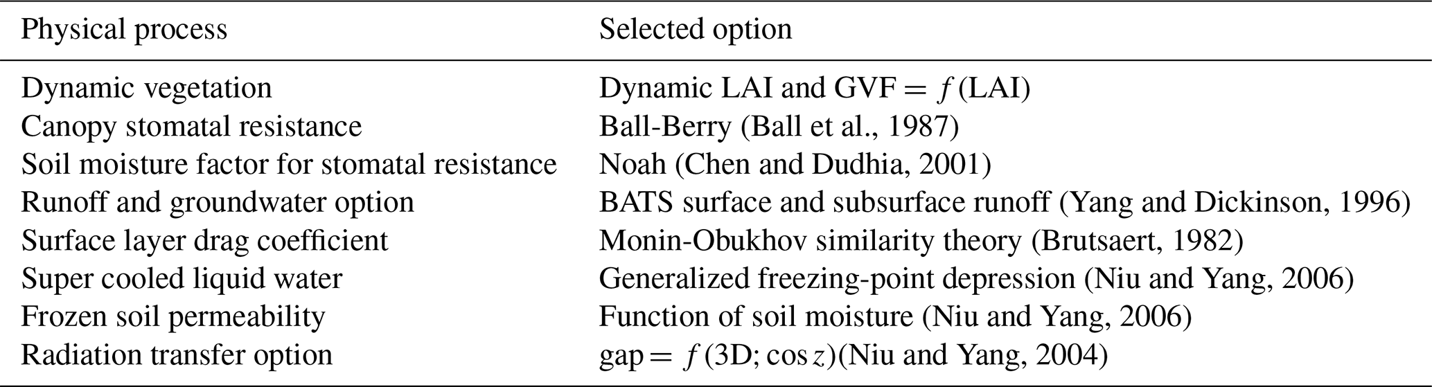
Figure C1 shows the average length (number of days) and the start of the growing season (day of year) for both models, as derived from the dynamic vegetation. The growing season corresponds to the period when irrigation is allowed (can be triggered in the model). For AquaCrop, the spatial patterns for the length and start of the growing season are identical (same spatial standard deviation). This is because the crop parameters related to the start and duration of senescence fix the end of the growing season on 24 September (23 September for leap years). The spatial patterns of the growing season lengths for the two models are different; some areas towards the western side of the domain have a short growing season for AquaCrop, but they stand out with the longest growing season for Noah-MP. This can be attributed to the fact that GVF drops only for a short period in winter and increases rapidly to high GVF_min values for Noah-MP. This also explains the typical earlier start of the growing season for Noah-MP compared to AquaCrop. In addition to an earlier start, the season ends later in the year, because irrigation causes an extended vegetation growth and harvest is not modeled (De Lannoy et al., 2024). In general, the start of the growing season shows more variability for AquaCrop, where the difference between the latest and earliest start date at one location is on average 33 d, compared to 28 d for Noah-MP.

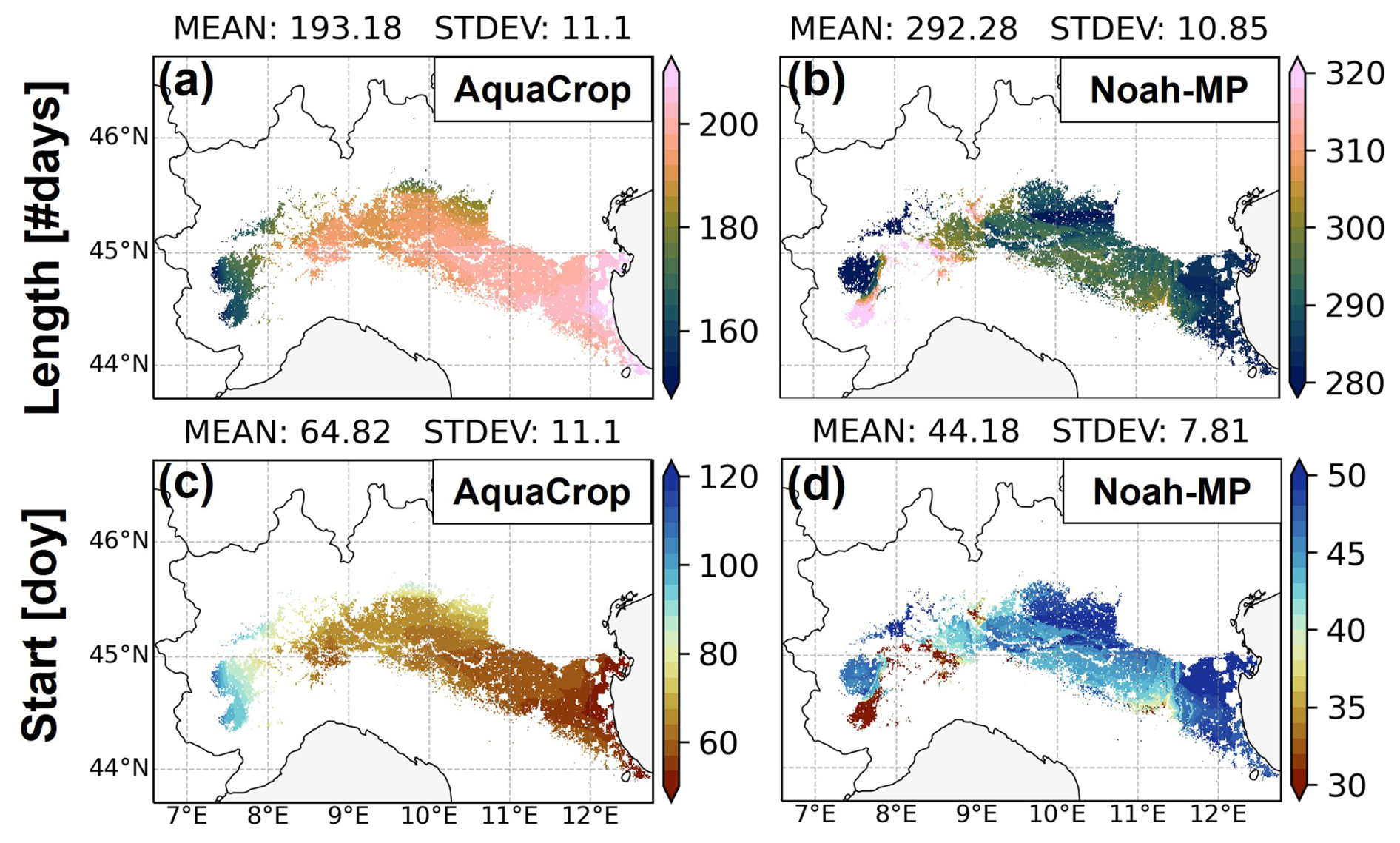
Figure C1 Average length in number of days [#days] and start as day of the year [doy] of the growing season over 8 years (2015–2022) for AquaCrop and Noah-MP. Note the different ranges in colorbars.

Appendix D: Evaluation with SMAP SSM

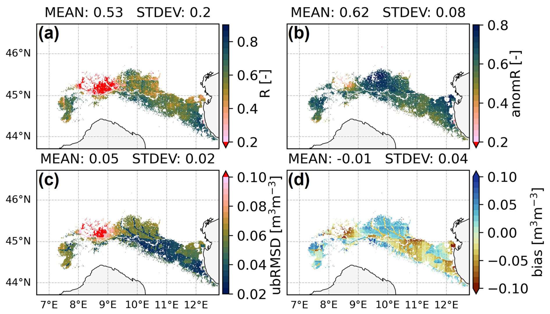
Figure D1 Maps of R [–], anomR [–], ubRMSD [m³ m⁻³], and bias [m³ m⁻³] of the evaluation of AquaCrop 15 d SSM estimates against SMAP 1 km SSM for March through September.

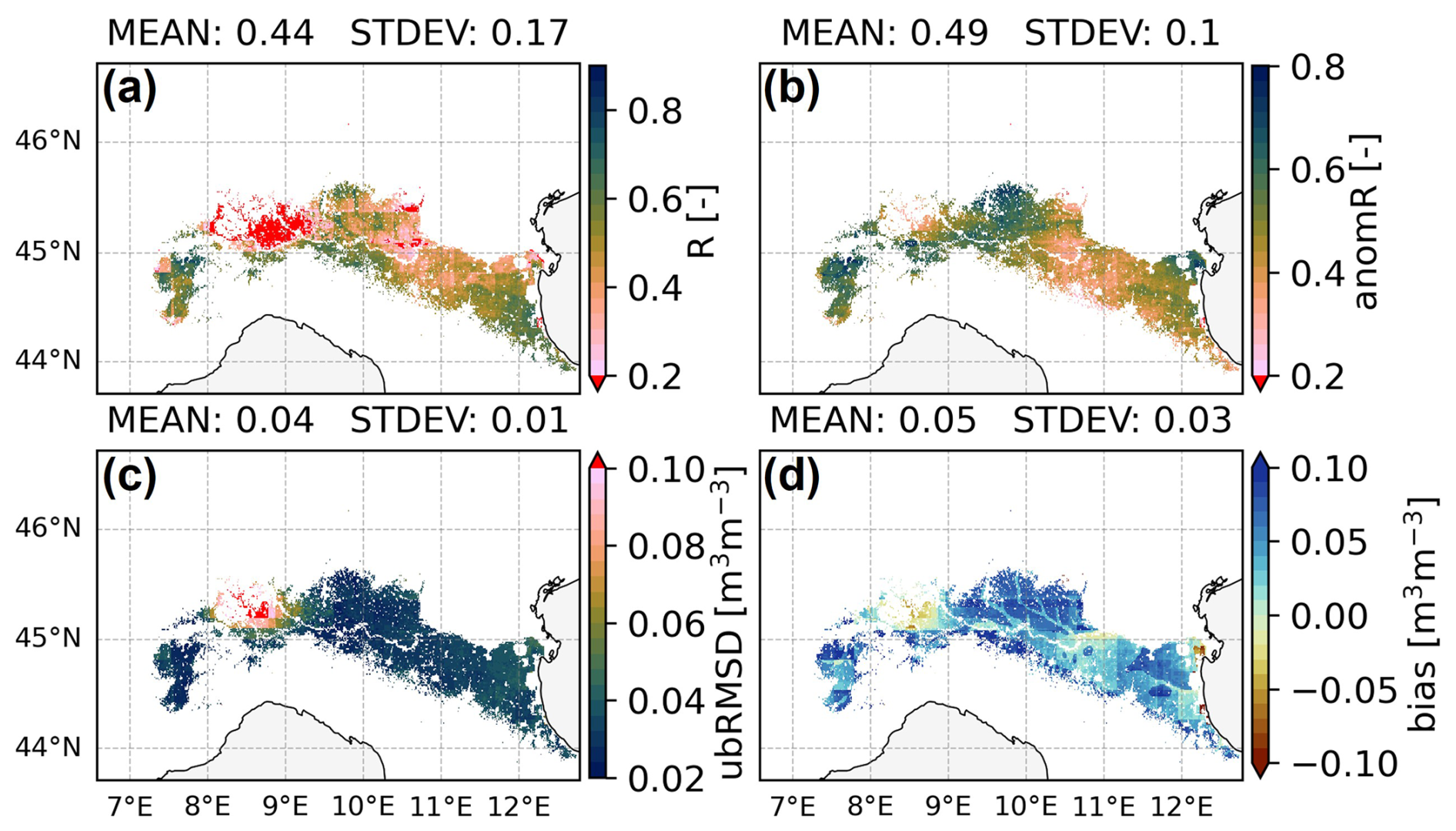
Figure D2 Maps of R [–], anomR [–], ubRMSD [m³ m⁻³], and bias [m³ m⁻³] of the evaluation of Noah-MP 15 d SSM estimates against SMAP 1 km SSM for March through September.

Appendix E: Evaluation with CGLS DMP

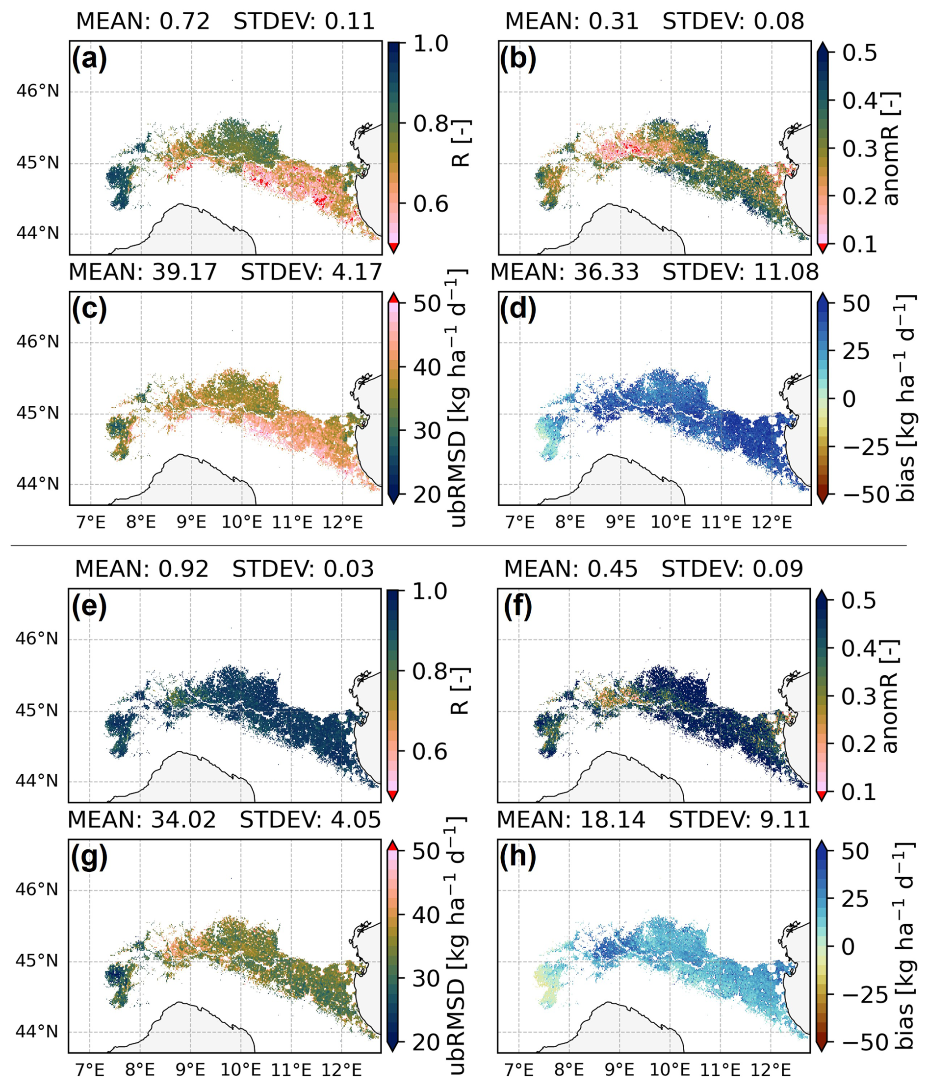
Figure E1 Maps of R [–], anomR [–], ubRMSD [$\mathrm{kg}{\mathrm{ha}}^{-\mathrm{1}}{\mathrm{d}}^{-\mathrm{1}}$], and bias [$\mathrm{kg}{\mathrm{ha}}^{-\mathrm{1}}{\mathrm{d}}^{-\mathrm{1}}$] of the evaluation of AquaCrop biomass estimates against 10 d CGLS DMP. The top 4 maps (a–d) correspond to the evaluation over the months March through September, and the bottom panels (e–h) are the evaluation of the months January through June.

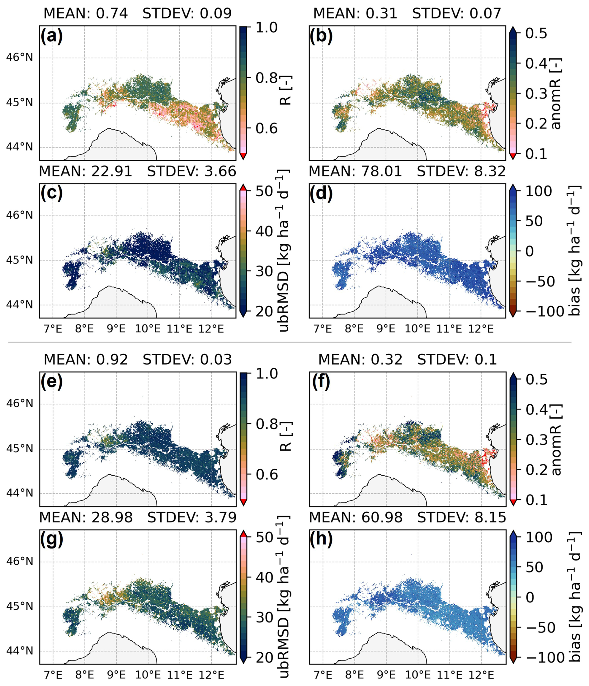
Figure E2 Maps of R [–], anomR [–], ubRMSD [$\mathrm{kg}{\mathrm{ha}}^{-\mathrm{1}}{\mathrm{d}}^{-\mathrm{1}}$], and bias [$\mathrm{kg}{\mathrm{ha}}^{-\mathrm{1}}{\mathrm{d}}^{-\mathrm{1}}$] of the evaluation of Noah-MP NPP estimates against 10 d CGLS DMP. The top 4 maps (a–d) correspond to the evaluation over the months March through September, and the bottom panels (e–h) are the evaluation of the months January through June.

Appendix F: Evaluation with SenET

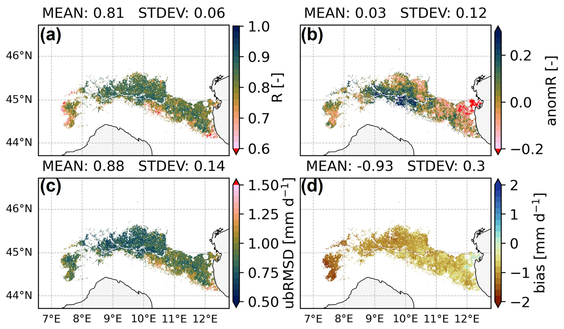
Figure F1 Maps of R [–], anomR [–], ubRMSD [mm d⁻¹], and bias [mm d⁻¹] of the evaluation of AquaCrop 15 d ET estimates against SenET for March through September.

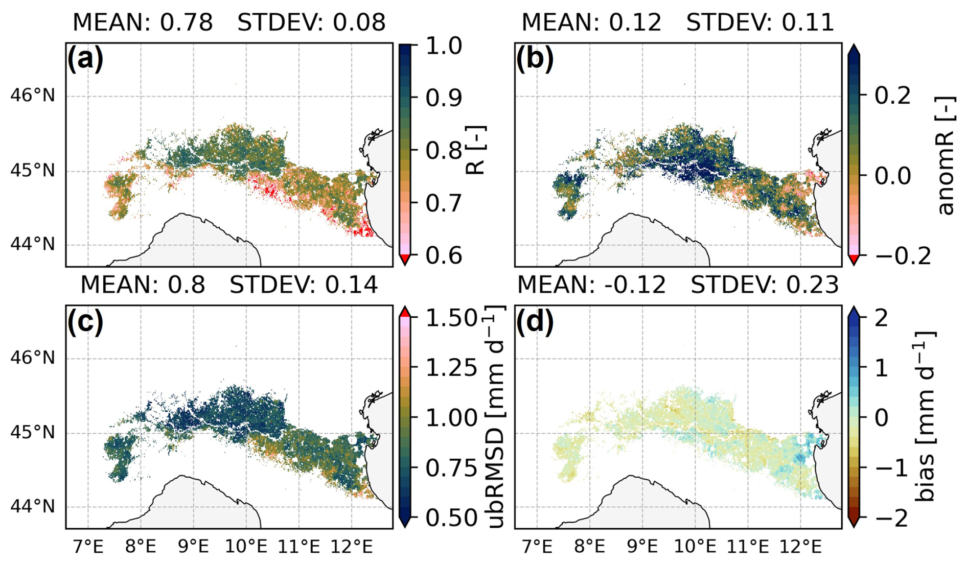
Figure F2 Maps of R [–], anomR [–], ubRMSD [mm d⁻¹], and bias [mm d⁻¹] of the evaluation of Noah-MP 15 d ET estimates against SenET for March through September.

Appendix G: ET time series

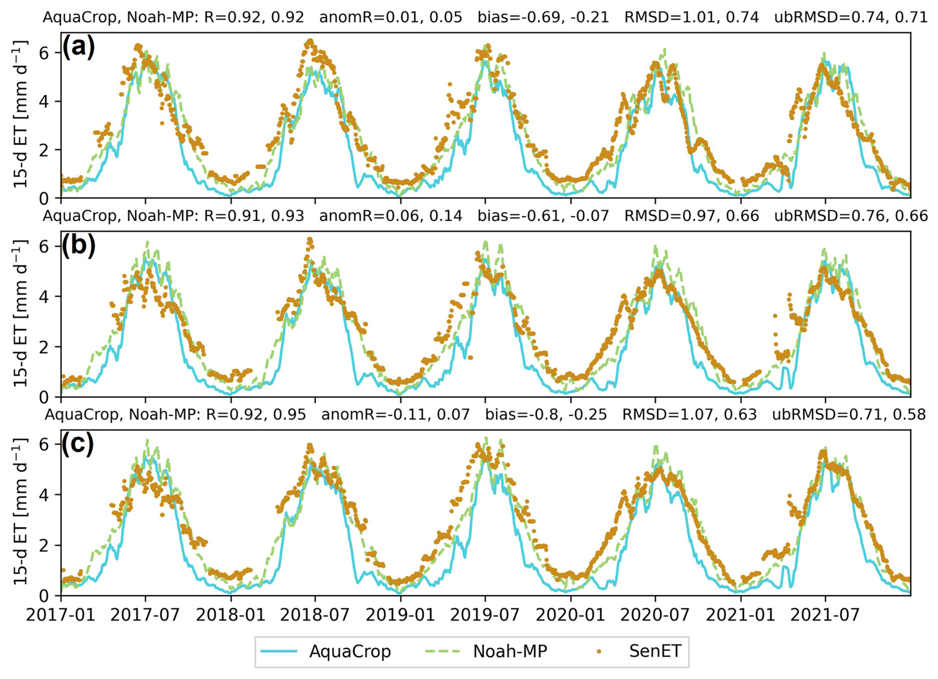
Figure G1 Time series of AquaCrop and Noah-MP 15 d ET estimates along with SenET retrievals for (a) Budrio (1 pixel), (b) Faenza San Silvestro (3 pixels), and (c) Faenza Formellino (8 pixels). The metrics are computed over the full year.

Appendix H: Irrigation evaluation over Faenza fields

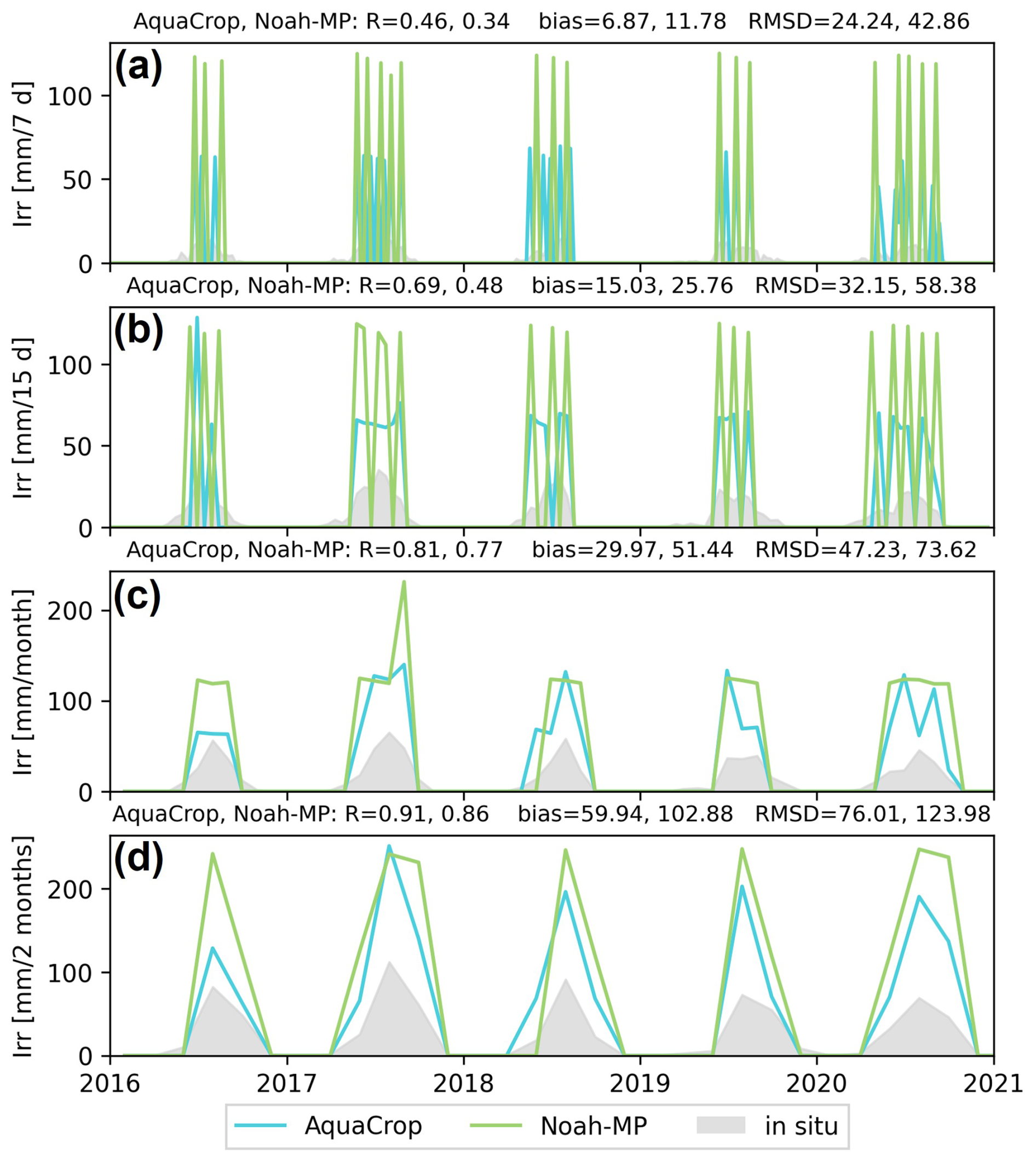
Figure H1 Irrigation time series for the Faenza San Silvestro fields aggregated over different time intervals. The metrics are computed for the months March through September. Note that the in situ irrigation amounts between mid-August and December 2018 are missing and the simulated data were masked accordingly.

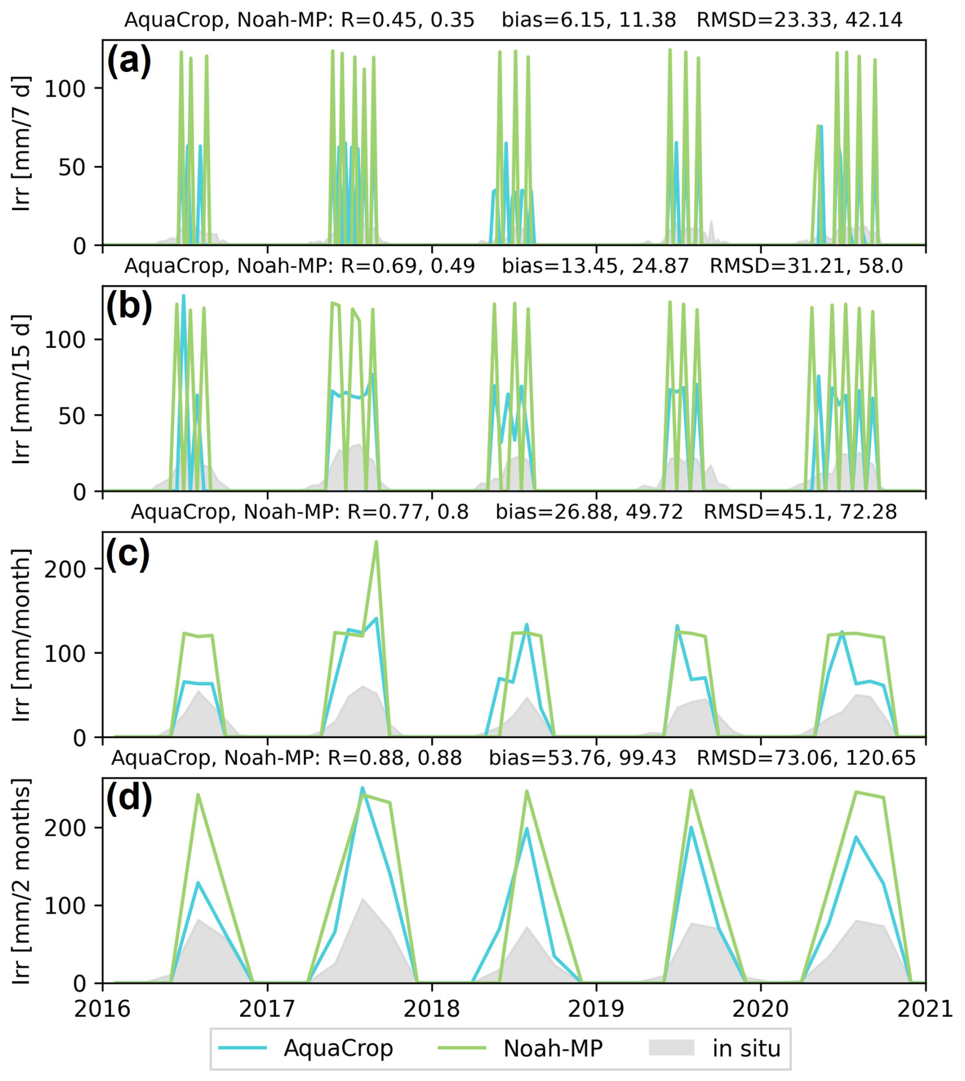
Figure H2 Irrigation time series for the Faneza Formellino fields aggregated over different time intervals. The metrics are computed for the months March through September. Note that the in situ irrigation amounts between mid-August and December 2018 are missing and the simulated data were masked accordingly.