Hyper-resolution large-scale hydrological modelling benefits from improved process representation in mountain regions

Many of the world's major rivers originate in mountain regions, and a large fraction of the global population relies on these regions for their water supply. The hydrological cycle of mountain regions and their dependent downstream regions are often studied using large-scale to global hydrological models (LHMs). The increasing spatial resolution of these models allows for improved representation of complex mountain topography, but existing model deficiencies in cold and high-elevation regions limit potential model performance gains. Such model performance gains might be realized by investing in a better representation of hydrological processes that are relevant in mountain regions such as snow accumulation and snowmelt. However, how much improved process representation would increase LHM performance remains largely unquantified. Here, we set up the hyper-resolution 30 arcsec (approx. 1 km) global hydrological model PCR-GLOBWB 2.0 (PCRaster Global Water Balance) over the larger Alpine domain and implement several changes to make it better suited for representing hydrological processes in mountain regions. These changes include (a) the use of novel high-resolution meteorological forcing datasets, (b) an extended snow module based on a seasonally varying degree-day factor and an exponential melt function, (c) a regional calibration of the snow module against a snow reanalysis product, (d) a new integrated glacier module, and (e) an adjusted runoff partitioning scheme that increases the contributions to the fast-runoff components in the soil. Our evaluation of the effect of these different adjustments on model performance for discharge shows that, while the meteorological forcing has a major effect on discharge simulations, it results in a mixed pattern of performance gains and losses over the domain. In addition, the structural and parametric changes, i.e. the snow module modification, glacier representation, and runoff partitioning, improve discharge simulations in mountain regions: the snow module modification leads to an improved representation of the snowmelt peak for high-elevation catchments, the glacier module supplies additional water to glacierized catchments, and runoff partitioning in the soil improves the representation of streamflow in flashy catchments at lower elevations. We use these insights to present a new setup of the large-scale and hyper-resolution PCR-GLOBWB 2.0 model that is better suited to studying hydrological processes in and beyond mountain regions around the world.

1 Introduction

Mountain regions play a critical role in supplying water to almost 2 billion people living in downstream regions and are therefore often referred to as the “water towers” of the world (Viviroli et al., 2007; Immerzeel et al., 2010, 2020). Water storage in snow and glaciers – or a lack thereof – is particularly important for drought development and recovery: the snow drought in the Italian Alps in 2022 developed into a streamflow drought downstream and affected many communities in the Po Plain (Colombo et al., 2023), whereas Alpine glaciers provided surrounding rivers with surplus meltwater during the 2003 Central European Drought due to very negative mass balances (Van Tiel et al., 2023). Hydrological processes in mountain regions thus have an over-proportional footprint well beyond mountain ranges. Therefore, considering the driving hydrological processes in mountain regions such as snow accumulation or glacier melt is critical when studying hydro-systems in mountains and their dependent downstream regions.

Large-scale or global hydrological models (LHMs) are often used to study mountain hydro-systems and their dependent downstream areas (e.g. Viviroli et al., 2007, 2020; Khanal et al., 2021) but also to examine many other hydrological systems that exceed the scale of individual catchments. Example applications of such models include water resources (e.g. Dolan et al., 2021; Leijnse et al., 2024) and climate change impact assessments, such as those performed within the Inter-Sectoral Impact Model Intercomparison Project (ISIMIP; Warszawski et al., 2014). However, the coarse spatial resolution of many large-scale models – often tens of kilometres – limits the usefulness of their output for policymakers, who are often interested in more detailed information. This scale gap triggered a call for hyper-resolution, kilometre-scale models that are applicable at continental to global scales (Wood et al., 2011; Bierkens et al., 2015). This call has been addressed by an increasing number of studies: proposed model solutions include the 1 km setup of the ParFlow model for the Contiguous United States (Yang et al., 2023) or the PCR-GLOBWB 2.0 model over Europe at a similar resolution (30 arcsec; Hoch et al., 2023), which Van Jaarsveld et al. (2025) recently used to perform a first global run at a hyper-resolution.

At coarse spatial resolutions, there is ample evidence suggesting that LHMs do not accurately capture mountain processes. Recent evaluations found that global hydrological and land surface models show particularly poor performance at high elevations (Heinicke et al., 2024) and in cold climates (Gädeke et al., 2020; Hou et al., 2023) compared to in other regions. One of the underlying issues is the extreme heterogeneity in mountain regions in terms of, for example, topography, meteorology, and soil types. Hyper-resolution models are expected to better represent this heterogeneity and could thus improve model performance in mountain catchments, e.g. for snow simulations (Malle et al., 2024). However, to realize such increased model performance, the processes at play also need to be represented and parameterized with sufficient detail and accuracy. Part of the reduced performance in mountain regions can indeed be attributed to issues with process representation, as indicated by misrepresentations of both the volume and timing of snowmelt peaks, as well as poor performance in basins where glaciers are not represented by the models (Gädeke et al., 2020). Furthermore, neglecting glaciers or snow transport also leads to the formation of unrealistic “snow towers” at high elevations (Freudiger et al., 2017; Hoch et al., 2023). Several studies thus suggest that improving cryospheric process representation should be a focus of further LHM development (Gädeke et al., 2020; Heinicke et al., 2024; Van Jaarsveld et al., 2025).

Many LHMs represent snowmelt using a temperature index model which relates melt to air temperature via a degree-day factor (DDF; Telteu et al., 2021). Even though full energy balance models are becoming more popular, especially at the catchment scale, temperature index models remain widely used because they come with reduced computational demand, require minimal meteorological forcing, and are accurate when calibrated (e.g. Hock, 2003; Magnusson et al., 2015). However, LHMs often use very simplistic temperature index schemes, e.g. by using only a time-constant DDF or by omitting calibration (e.g. Gosling and Arnell, 2011; Sutanudjaja et al., 2018; Müller Schmied et al., 2021; Stacke and Hagemann, 2021). Snow module comparisons at the catchment scale suggest that performance gains might be achieved by changes in the structure of the snow module (Girons Lopez et al., 2020).

Proper evaluation of such improvements hinges on the availability of high-quality reference data to compare how snow is represented by different snow module structures. Evaluations of snow processes in LHMs are often performed against global products representing snow water equivalent (SWE) or snow cover fraction derived from satellite measurements or reanalyses (e.g. Schellekens et al., 2017; Gädeke et al., 2020; Van Jaarsveld et al., 2025). Of the two, SWE is hydrologically the most relevant in regions with seasonal snow cover, but SWE reanalysis products often have too coarse a spatial resolution (often 25 km or more) to be representative of mountain regions (Mortimer et al., 2020). In addition, the coarse model resolutions of LHMs themselves prevented direct comparisons of SWE simulations with SWE estimates at individual snow measurement stations before the era of high-resolution modelling. Now, the higher spatial resolutions of LHMs and new detailed regional SWE reanalysis products (e.g. Mott et al., 2023; Olefs et al., 2020) enable such direct SWE comparisons with the outputs of LHMs at a regional scale for mountain regions.

Whereas snow modules are present in most LHMs, many models have largely neglected glaciers (Gädeke et al., 2020; Telteu et al., 2021; Hanus et al., 2024). Glaciers can be an important additional water source during their melt season; on average, the glacier storage change contribution to total runoff ranges from 4 % in the river Danube at Ceatal Izmail in September to 25 % for the river Rhône at Beaucaire in August (Huss, 2011), and such contributions can become especially important during drought (Van Tiel et al., 2021, 2023). Including glaciers in hydrological models can thus potentially improve discharge simulations (Wiersma et al., 2022; Hanus et al., 2024), although such improvements will be limited to the summer months and to regions with substantial glacier cover. Glaciers are represented in hydrological modelling in two ways, namely by (a) including an internal glacier module in the hydrological model (“integrated models”) or (b) using the output from an external glacier model as the input into the hydrological model (i.e. coupling the models; “coupled models”). An example of a coupled model is the setup created by Hanus et al. (2024), who used output from the Open Global Glacier Model (OGGM; Maussion et al., 2019) as the input into the Community Water Model V1.08 (CWatM; Burek et al., 2020). Similarly, Wiersma et al. (2022) coupled the Global Glacier Evolution Model (GloGEM; Huss and Hock, 2015) to PCR-GLOBWB 2.0. An example of an integrated model at the catchment scale is HBV-light (Hydrologiska Byråns Vattenavdelning) (Seibert and Vis, 2012; Seibert et al., 2018a), which calculates glacier mass balance, area evolution, and runoff internally. The external glacier models used in coupled model setups generally have more detailed process representation or more detailed calibration than would be feasible for integrated glacier modelling in LHMs. Still, we argue that integrated models can also have certain advantages over coupled models. First, integrated glacier modules are physically consistent with the surrounding model framework, which is not necessarily the case for externally coupled glacier models. For example, large-scale glacier models may use different precipitation correction factors for each individual glacier, which is inconsistent with the precipitation in non-glacierized grid cells. Furthermore, glacier geometries evolve over time, and assumptions have to be made regarding how increases in the non-glacierized area are dealt with by the hydrological model (e.g. Hanus et al., 2024, assume the same relative glacier area change over all cells covered by a glacier, whereas, in reality, area changes mainly affect the glacier terminus). Second, integrated models can be more flexible: an integrated module can – in contrast to coupled models – be run simultaneously with the hydrological model and avoids the coupling steps related to transferring data between the models. This could make integrated models easy to use when forcing them with an ensemble of meteorological forcing datasets.

Aside from snow and glaciers, rivers in mountainous or hilly regions often respond rapidly to local rainfall events, leading to “flashy” discharge behaviour. These flashy responses are caused by the heavy precipitation, thin soils, and steep slopes that characterize these regions and that make these regions susceptible to floods (Weingartner et al., 2003). Simplifications in the representation of soil processes and runoff production seem to limit LHM performance in flashier basins (Gharari et al., 2019). Generally, LHMs split the soil into a few layers that store and exchange water, but the exact details can vary significantly: each model has a different number of soil layers (e.g. CWatM: three layers, Burek et al., 2020; WaterGAP: one soil layer, Müller Schmied et al., 2021), and these layers can have different thicknesses (e.g. CWatM: upper layer is 5 cm thick, as in Burek et al., 2020; WaterGAP: soil is 0.1 up to 4 m, as in Telteu et al., 2021). Interaction between these soil layers determines how water is partitioned over different runoff processes. Most LHMs are not locally calibrated (Telteu et al., 2021), relying instead on a standard parameterization which should avoid obscuring structural deficiencies (Refsgaard and Storm, 1996; Andréassian et al., 2012). Without representing additional soil processes, we hypothesize that hyper-resolution LHMs can already realize further performance gains by reconsidering standard parameterizations (Hoch et al., 2023). For example, on steeper slopes, the contribution of near-surface runoff components is larger (Weingartner et al., 2003). Changing how water fluxes from the soil are partitioned across different processes that contribute to discharge (e.g. reduced groundwater recharge and increased saturation excess and interflow) could thus potentially capture more flashy behaviour. This could also improve the local relevance of these models, although their main focus will remain the larger catchments.

Nevertheless, any potential gains in model performance due to improved process representation or parameterization are constrained by the quality of the model input. It is thus important that such conditions be met first. Hydrological modelling is indeed sensitive to the meteorological forcing dataset used as input (e.g. Raimonet et al., 2017; Tang et al., 2023; Gebrechorkos et al., 2024). For hyper-resolution LHMs, the horizontal resolution of the meteorological forcing dataset is of particular importance as using too coarse a meteorological forcing can severely reduce potential performance gains when it comes to moving towards hyper-resolution hydrological modelling (Hoch et al., 2023). High-resolution meteorological reanalysis products can be derived by downscaling coarser products by exploiting statistical, physical, or heuristic relationships or by using dynamically generated regional reanalysis products. Both types of downscaled products often outperform coarser global reanalysis products, e.g. in representing precipitation (e.g. Karger et al., 2021b; Keller and Wahl, 2021). These products should also represent temperature gradients with elevation in more detail, which can be important for snow modelling (Malle et al., 2024). However, a main difference between the two types of downscaling is that regional reanalysis products also explicitly represent higher-resolution atmospheric dynamics. While Hoch et al. (2023) studied the effect of the spatial resolution of the meteorological forcing dataset (using statistical downscaling) on hyper-resolution LHM performance, it remains to be assessed how the exact procedure of deriving data at higher spatial resolutions influences model performance. Furthermore, despite improved resolutions, precipitation products in particular are known for their large uncertainties over mountain regions (e.g. Isotta et al., 2015; Gampe and Ludwig, 2017; Bandhauer et al., 2022). It is thus important to assess how sensitive hydrological model performance in mountain regions is to the specific biases and large uncertainties of meteorological forcing datasets.

While large-scale hydrological simulations at higher spatial resolutions have become feasible thanks to increasingly available computational resources, it remains unclear by how much hydrological simulations can improve when combining such high-resolution models with the latest generation of meteorological forcing datasets and improved process representation. Therefore, here, we aim to explore the effect of (1) using different meteorological datasets, (2) improving snow and glacier representations, and (3) changing runoff partitioning in the soil on discharge simulations in PCR-GLOBWB 2.0. We focus on the larger Alpine region as an example of a mountain region that is normally implicitly simulated by LHMs. A similar setup can, in principle, be applied at larger scales. While more detailed hydrological modelling approaches are available for the Alps at the national or catchment scale, the Alps are very rarely studied as a whole at a similarly high spatial resolution, which inhibits comparisons between different regions within the Alps. We hypothesize that hyper-resolution LHM performance for discharge in mountain regions will increase by (H1) using forcing products that include a representation of smaller-scale atmospheric dynamics compared to other forcing products; (H2) improving the representation of mountain hydrological processes, such as snowmelt and ice melt; and (H3) reviewing and adjusting standard parameterizations. To test these hypotheses, we first assess how strongly discharge simulations are affected by the meteorological forcing chosen to drive the model. Second, we quantify the effect of structural changes in the model setup on model performance, namely by expanding the existing snow module and adding a new glacier module. Third, we study the effect of parameter changes on model performance by calibrating snow module parameters against a detailed regional SWE reanalysis product with assimilated observations and changing parameters controlling the volumes of soil compartments.

2 Methods

2.1 Model setup and study outline

We use the PCR-GLOBWB 2.0 model (Sutanudjaja et al., 2018) in the 30 arcsec setup developed by Hoch et al. (2023) (approx. 1 km at the Equator and 650 m in the longitudinal direction in the Alps). The model runs at a daily time step. PCR-GLOBWB 2.0 is a global hydrological model and contains different modules, which represent both natural processes related to vegetation, snow, soil, groundwater, and river routing and anthropogenic processes such as human water use and irrigation.

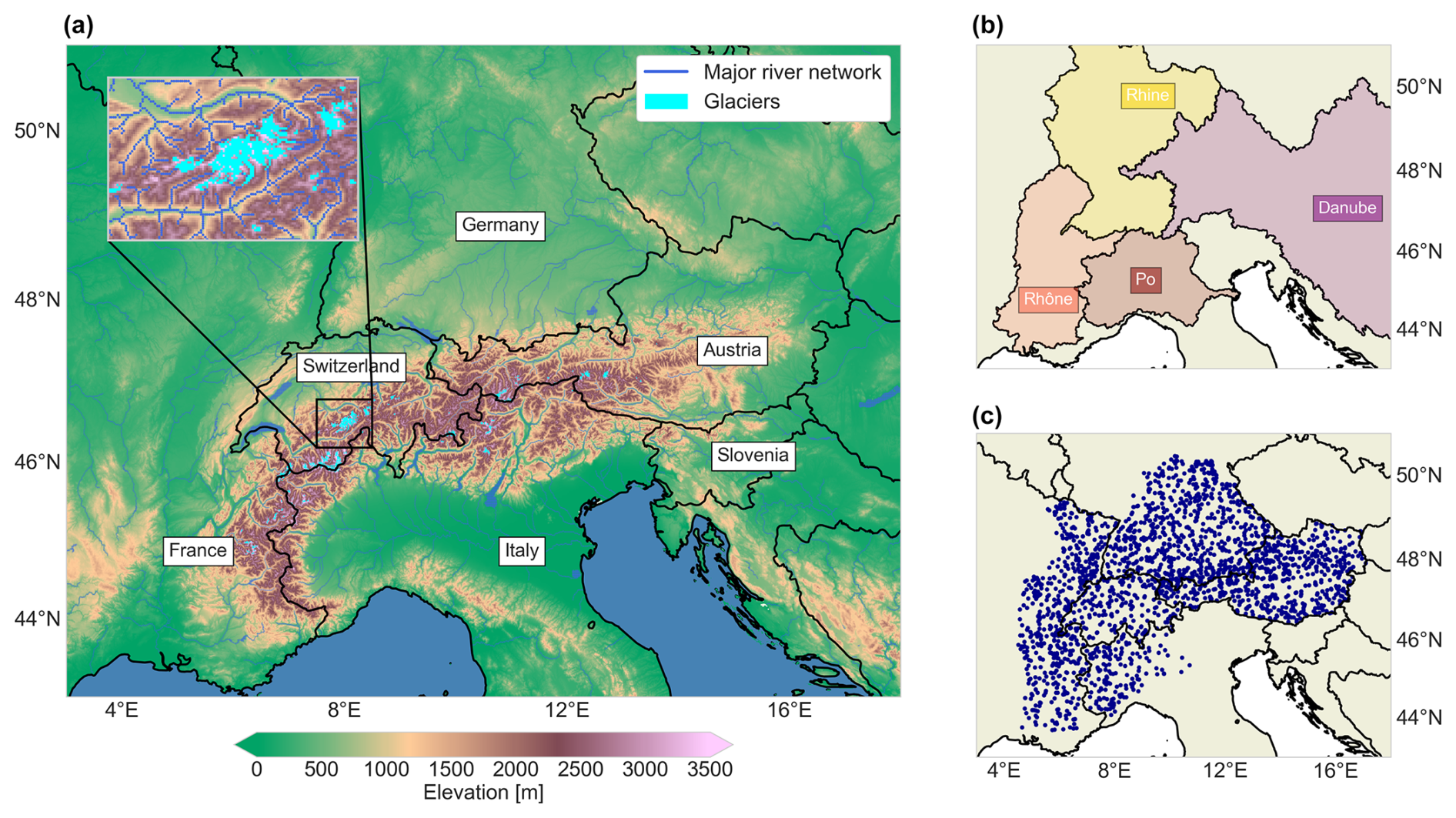
Figure 1 (a) Overview of the model domain, highlighting the larger Alpine countries, major rivers, topography, and glaciers. The inset map shows the area around the Aletsch Glacier (the largest glacier in the Alps) in more detail. Elevations are derived from the upscaled MERIT Hydro DEM (Yamazaki et al., 2019). (b) The larger river basins of the Alpine rivers, indicated with a slight shading. (c) The discharge stations used to evaluate the model (see Sect. 2.2).

Here, we use a regional model setup (latitude: 43–51°, longitude: 3–18°) covering the Alps and the upstream parts of the catchments of four major central European rivers (i.e. the Rhone, Rhine, Danube, and Po; Fig. 1). We focus on the period 1990–2019 as all forcing datasets are available for this time period, and initial glacier volumes are often only available for around the year 2000.

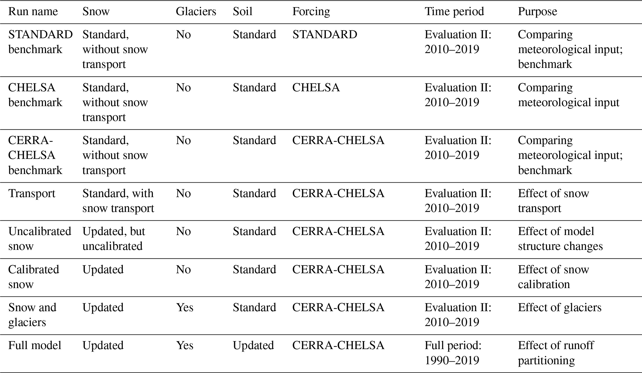
We implement the different forcing datasets and model changes in a step-by-step manner and thus perform several model runs. A schematic overview and further details on the sequential model runs performed in this study are provided in Fig. 2 and Table 1, respectively.

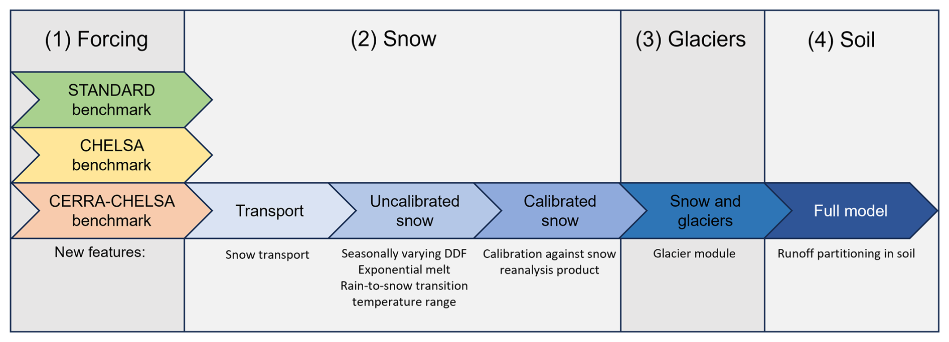
Figure 2 Overview of the different model runs performed in this study. (1) The standard model setup with standard parameterization is our benchmark model, and we run it with different forcing datasets. (2) Several changes are implemented in the snow module in different runs. (3) A new glacier module is added. (4) Runoff partitioning is adjusted, which is the final model change.

Table 1 List of the sequential model runs performed within this study.

2.2 Datasets

2.2.1 Model input

To quantify the sensitivity of hydrological models to the choice of the forcing dataset, we assess how discharge simulations vary under different meteorological forcing datasets. We focus on the input variables of precipitation rate and near-surface air temperature as these are available for a wide range of potential meteorological datasets. Evaporation is then calculated within PCR-GLOBWB 2.0 using the method from Hamon (1963). For our comparison, we use the following meteorological datasets: (1) the “STANDARD” input for hyper-resolution PCR-GLOBWB 2.0; (2) Climatologies at High resolution for the Earth’s Land Surface Areas v2.1 (CHELSA); and (3) CERRA-CHELSA, a mixed dataset with temperature from the Copernicus European Regional ReAnalysis (CERRA) further downscaled using the CHELSA algorithm and precipitation data directly from CERRA-Land.

The STANDARD forcing was created by Van Jaarsveld et al. (2025). They created an internal meteorological downscaling scheme in PCR-GLOBWB 2.0. This scheme uses coarser-scale meteorological input, in this case the W5E5 v2.0 (WFDE5 over land merged with ERA5 over the ocean) dataset (Lange et al., 2021), which has a spatial resolution of 0.5°. This coarser dataset is then downscaled to 30 arcsec spatial resolution using monthly climatologies from CHELSA-BIOCLIM+ (Climatologies at High resolution for the Earth's Land Surface Areas – bioclimatic variables plus) (Karger et al., 2017; Brun et al., 2022b). CHELSA (Karger et al., 2017, 2021a) is a downscaled reanalysis product based on the ERA5 product (Hersbach et al., 2020). CHELSA uses heuristic and physical relationships to downscale these forcing data to 30 arcsec spatial resolution. Downscaling is performed using topography, atmospheric lapse rates (for temperature; Karger et al., 2023), spatial wind fields, and the height of the boundary layer (for precipitation; Karger et al., 2021b). Finally, CERRA (Schimanke et al., 2021; Ridal et al., 2024) is a regional reanalysis product over Europe provided at 5.5 km spatial resolution (approx. 180 arcsec). CERRA-Land is the associated surface analysis (Verrelle et al., 2022), which also includes additional data assimilation of precipitation observations. We decided to use precipitation directly from CERRA-Land since this dataset is already near the effective resolution of precipitation and because the terrain effect could be over-represented by downscaling the data further (Daly et al., 1997; Karger et al., 2021b, use 3 km). In contrast, near-surface air temperature can be further downscaled to generate more accurate spatial melt patterns at 30 arcsec resolution. Therefore, we created a new CHELSA-CERRA temperature dataset, for which temperature was taken from the CERRA dataset and was downscaled using the topographical CHELSA v2.1 algorithm (Karger et al., 2023). For simplicity, we refer to the combined meteorological product as CERRA-CHELSA in the remainder of this paper.

To implement a new glacier module, we used the locations of the existing glaciers and their initial ice thickness using the consensus estimate from Farinotti et al. (2019), representative of the year 2003 for most glaciers. To our knowledge, there are no estimates of glacier volumes available that go further back in time and that cover all glaciers at the global, continental, or Alpine scale. This glacier volume dataset has a varying spatial resolution (max. 200 m) and has previously also been used to initialize glaciers for the same study period by Hanus et al. (2024).

2.2.2 Evaluation and calibration data

Within this study, we use several reference datasets against which we compare model inputs (forcing) and outputs such as streamflow, SWE, and glacier changes (Table ). As a reference meteorological dataset, we use the Alpine Gridded Precipitation Dataset (APGD; Isotta et al., 2014). This is a gridded product at 5 km spatial resolution covering the period 1971–2008 and is based on interpolated rain gauge data over the Alps. We choose this dataset as a reference because, unlike the other datasets, it is specifically created for the Alps, does not use reanalyses, and has been used as a reference meteorological dataset before (Isotta et al., 2015). However, the dataset was not corrected for undercatch (which can be tens of percentage points in the Alps; Sevruk, 1985). Please note that we do not use this dataset as the forcing input since LHMs are generally run at larger scales, and, therefore, we used forcing products that are at least available at the continental scale.

Van Jaarsveld et al. (2025)Karger et al. (2021a, b, 2023)Schimanke et al. (2021); Verrelle et al. (2022); Ridal et al. (2024)Isotta et al. (2014); Isotta and Frei (2013)Schlemper et al. (2024)Mott et al. (2023); Mott (2023)Olefs et al. (2020)Copernicus Climate Change Service (2019)Verrelle et al. (2022)Fontrodona-Bach et al. (2023b)Hugonnet et al. (2021a)World Glacier Monitoring Service (WGMS) (2023)Glacier Monitoring Switzerland (GLAMOS) (2022)Farinotti et al. (2019)Zekollari et al. (2020)Raup et al. (2007); GLIMS Consortium (2018)Pfeffer et al. (2014); RGI Consortium (2017)Gruber et al. (2019); Dorigo et al. (2017); Preimesberger et al. (2021); Dorigo et al. (2023)Yamazaki et al. (2019)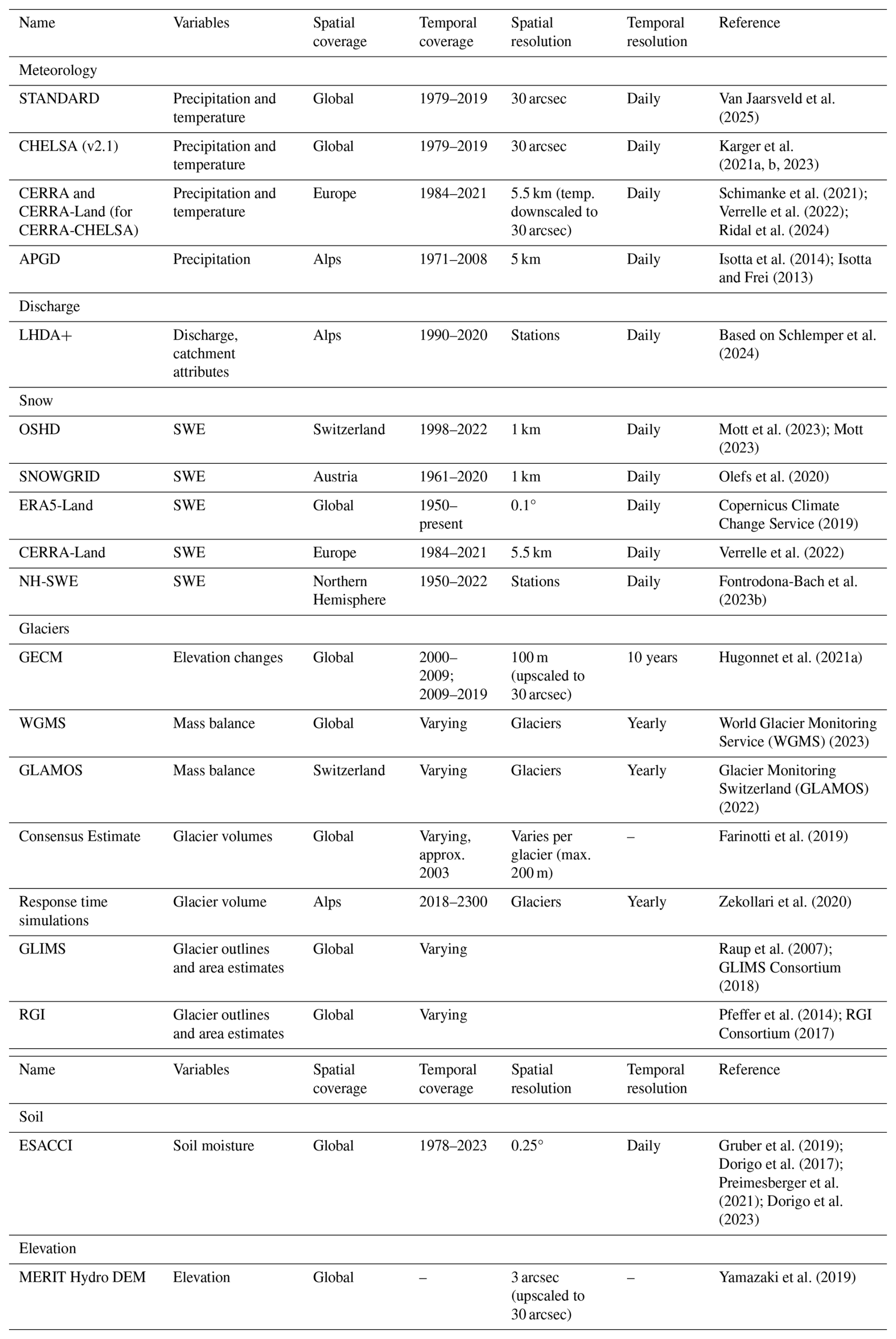

Table 2 List of used datasets and their description.

Reference measurements of discharge in rivers around the Alps are taken from both national and regional agencies (sources listed in Table A1 in Appendix A). We only select stations in the basins of the Po, Rhine, Rhone, and Danube rivers, leaving us with 2167 stations in total for the period 1990–2019. Please note that, for evaluations, we only use stations that have at least 3 years of data over the considered evaluation period (see Sect. 2.4). Since this dataset is an extended and updated version of the Large-sample hydro-meteorological dataset for the Alps (LHDA) from Schlemper et al. (2024), we refer to this dataset as LHDA+.

For SWE comparisons, we use a set of different SWE products. We use two 1 km gridded SWE regional reanalysis products at daily resolution, namely (1) a product by the Operational Snow Hydrological Service (OSHD) over (hydrological) Switzerland (Mott et al., 2023), which is available for the period 1998–2022, and (2) a product over Austria created with the SNOWGRID model (Olefs et al., 2013, 2020) for the period 1961–2020. Furthermore, we use the spatially much coarser SWE output from two atmospheric reanalysis products, namely CERRA-Land (5.5 km; 1984–2021) (Verrelle et al., 2022) and ERA5-Land (0.1° resolution (approx. 9 km); 1950–present) (Copernicus Climate Change Service, 2019). Finally, we use data from 1047 Alpine measurement stations where SWE was inferred from snow depth (Fontrodona-Bach et al., 2023b). For the locations, we refer the reader to Fig. S2 in the Supplement.

For glaciers, we use spatially explicit maps on glacier elevation changes derived from satellite observations at 100 m spatial resolution (Hugonnet et al., 2021a), that are then upscaled to match the 30 arcsec model resolution. Here, we refer to this dataset as the “Glacier elevation change maps” (GECM). We use maps from two 10-year periods, namely 2000–2009 and 2010–2019. We further use individual glacier mass balance measurements from World Glacier Monitoring Service (WGMS) (2023) and Glacier Monitoring Switzerland (GLAMOS) (2022). We only considered glaciers that have a minimum size of 3 km² (roughly four to five grid cells). Finally, we use glacier response time simulations from Zekollari et al. (2020) and glacier outlines and surface area estimates from Raup et al. (2007) and the GLIMS Consortium (2018) for further evaluation (see Sect. 2.4).

For soil moisture evaluation, we use the European Space Agency Climate Change Initiative (ESACCI) COMBINED soil moisture data v8.1 (Gruber et al., 2019; Dorigo et al., 2017; Preimesberger et al., 2021). The ESACCI dataset includes satellite observations of soil moisture in the top 5 cm of the soil at a resolution of 0.25°.

2.2.3 Ancillary data

To analyse what explains spatial patterns in model performance, we needed additional information on catchments, climate, or topography. For each of the catchments in LHDA+, the dataset includes a range of catchment characteristics. Catchment area and reservoirs (location and capacity) were both derived from government agencies or from existing databases (see Table A1). Although our reservoir database is more detailed than other large-scale databases such as the one by Lehner et al. (2005), it does not provide a complete overview of all reservoirs in the region. The fraction of the catchment covered by glaciers was computed from the Randolph Glacier Inventory (RGI) 6.0 (Pfeffer et al., 2014; RGI Consortium, 2017). Snowfall fraction and potential evapotranspiration per catchment were calculated based on our own simulated model output. Finally, for analyses that use elevation, we use the Multi-Error-Removed Improved-Terrain Hydro Digital Elevation Model (MERIT Hydro DEM) (Yamazaki et al., 2019). The MERIT Hydro DEM was upscaled from its original 3 arcsec resolution to 30 arcsec resolution by Hoch et al. (2023), who used it as the default DEM of the 30 arcsec version of PCR-GLOBWB 2.0.

2.3 Model development

Based on the initial regional model setup introduced in Sect. 2.1, we further develop the representation of cryospheric and soil processes to improve discharge simulations in mountain regions. We aim to find a regionally valid setup that works well for a larger domain and that is thus not directly fine-tuned for individual catchments, in line with the philosophy of many global hydrological models. The next few sections describe the structural changes made to the PCR-GLOBWB 2.0 model. The parameters used in the equations and any fixed values are listed in Table S1 in the Supplement. The calibration strategy for specific parameters is then further outlined in Sect. 2.3.4.

2.3.1 Snow module

The existing version of PCR-GLOBWB 2.0 includes a snow module consisting of a temperature index approach with a constant DDF. A temperature index model generally has the following form:

$$\begin{array}{}\text{(1)}& M=\text{DDF}\times (T-T_{\text{thresh}}),\end{array}$$

where M represents the melt rate (m d⁻¹), DDF represents the degree-day factor (m °C⁻¹ d⁻¹), T represents the daily average temperature (°C), and T_thresh represents the temperature threshold above which melt occurs. We build on this existing setup and expand it with elements of the snow model outlined in Magnusson et al. (2014), namely (1) a seasonally varying DDF, (2) exponential dependence on temperature, and (3) a rain-to-snowfall transition temperature range.

First, we replace the constant DDF with a seasonally varying one to capture the effects of changes in the solar declination throughout the year, following the approach outlined in Slater and Clark (2006):

$$\begin{array}{}\text{(2)}& \begin{array}{rl}\text{DDF}& ={\displaystyle \frac{{\text{DDF}}_{\text{max}}+{\text{DDF}}_{\text{min}}}{\mathrm{2}}}\\ & +\sin \left({\displaystyle \frac{k\mathrm{2}\mathit{\pi }}{\mathrm{366}}}\right)\left({\displaystyle \frac{{\text{DDF}}_{\text{max}}-{\text{DDF}}_{\text{min}}}{\mathrm{2}}}\right).\end{array}\end{array}$$

For the Northern Hemisphere, DDF_max is the degree-day factor on 21 June (summer solstice; m °C⁻¹ d⁻¹), and DDF_min is the degree-day factor on 22 December (winter solstice; m °C⁻¹ d⁻¹). k represents the day of the year since 21 March (equinox; –). Second, we implement an exponential relationship between temperature and melt following Magnusson et al. (2014). This formulation makes the melt more sensitive to increasing temperatures than under the assumption of a linear relationship and allows for limited melt below the threshold temperature to account for days when the average temperature is below the threshold temperature but the maximum temperature surpasses it.

$$\begin{array}{}\text{(3)}& \begin{array}{rl}M& =\text{DDF}{m}_{\text{m}}({\displaystyle \frac{T-T_{\text{thresh}}}{m_{\text{m}}}}\\ & +\ln \left(\mathrm{1}+\exp \left(-{\displaystyle \frac{T-T_{\text{thresh}}}{m_{\text{m}}}}\right)\right))\end{array}\end{array}$$

In the above, m_m is a parameter controlling the transition between melt and no melt (°C) and was kept constant by Magnusson et al. (2014).

Third, we adapt the snowfall and rainfall partitioning to account for snow and rainfall coincidence by creating a temperature transition zone where rainfall smoothly changes into snowfall (Magnusson et al., 2014):

$$\begin{array}{}\text{(4)}& P_{\text{snowfall}}={\displaystyle \frac{P}{\mathrm{1}+\exp \left(\frac{T-T_{\text{snowfall}}}{m_{\text{p}}}\right)}},\end{array}$$

where P_snowfall represents precipitation falling as snow (m d⁻¹), P represents total precipitation (m d⁻¹), T represents daily average temperature (°C), T_snowfall represents temperature below which most precipitation falls as snow (°C), and the parameter m_p determines the range where snow and rainfall co-occur (°C) and was derived from snowfall observations by Magnusson et al. (2014). Aside from additions to the snow module, we also ignore refreezing in the snowpack since previous analyses have shown that it did not improve simulations (Magnusson et al., 2014; Girons Lopez et al., 2020).

Furthermore, we also include the lateral snow transport scheme introduced by Van Jaarsveld et al. (2025) as a separate development step to better quantify its effect against the other development steps in the snow and glacier modules. Van Jaarsveld et al. (2025) implemented a lateral snow transport scheme based on Frey and Holzmann (2015) to avoid unrealistic snow accumulation at high elevations. This scheme transports part of the snow downhill based on the surface slope whenever the snow cover exceeds an SWE content of 0.625 m. This threshold is based on values for the forest snow-holding capacity and snow density in Frey and Holzmann (2015) using a similar approach as in CWatM (Burek et al., 2020). However, the snow that is transported should sometimes be part of glacier accumulation, which is why, here, we apply the lateral-transport scheme only outside of glaciers. When we introduce the glacier module, we thus restrict the lateral snow transport and apply it only to non-glacierized areas. This means that snow can only be transported from (a) a non-glacierized cell to a non-glacierized cell and (b) from a non-glacierized cell to a glacierized cell. There is no snow transport from a glacierized cell to either a glacierized cell or a non-glacierized cell. When snow is transported onto a glacierized cell, it becomes part of the snow cover on the glacier: it can thus reduce ice melt and become part of the glacier accumulation (Kuhn, 2003; Freudiger et al., 2017).

2.3.2 Glacier module

We introduce a new glacier module into PCR-GLOBWB 2.0. To create glacierized cells, we derive glacier geometries and volumes from ice thickness estimates by Farinotti et al. (2019). We then resample and regrid these volumes to the model raster of 30 arcsec, applying a correction factor to preserve the total ice volume of the glaciers. A cell is considered to be fully glacierized as soon as any ice is present in the grid cell and there are no partially glacierized cells.

Figure 3 Schematic overview of the glacier module and its interaction with the snow module.

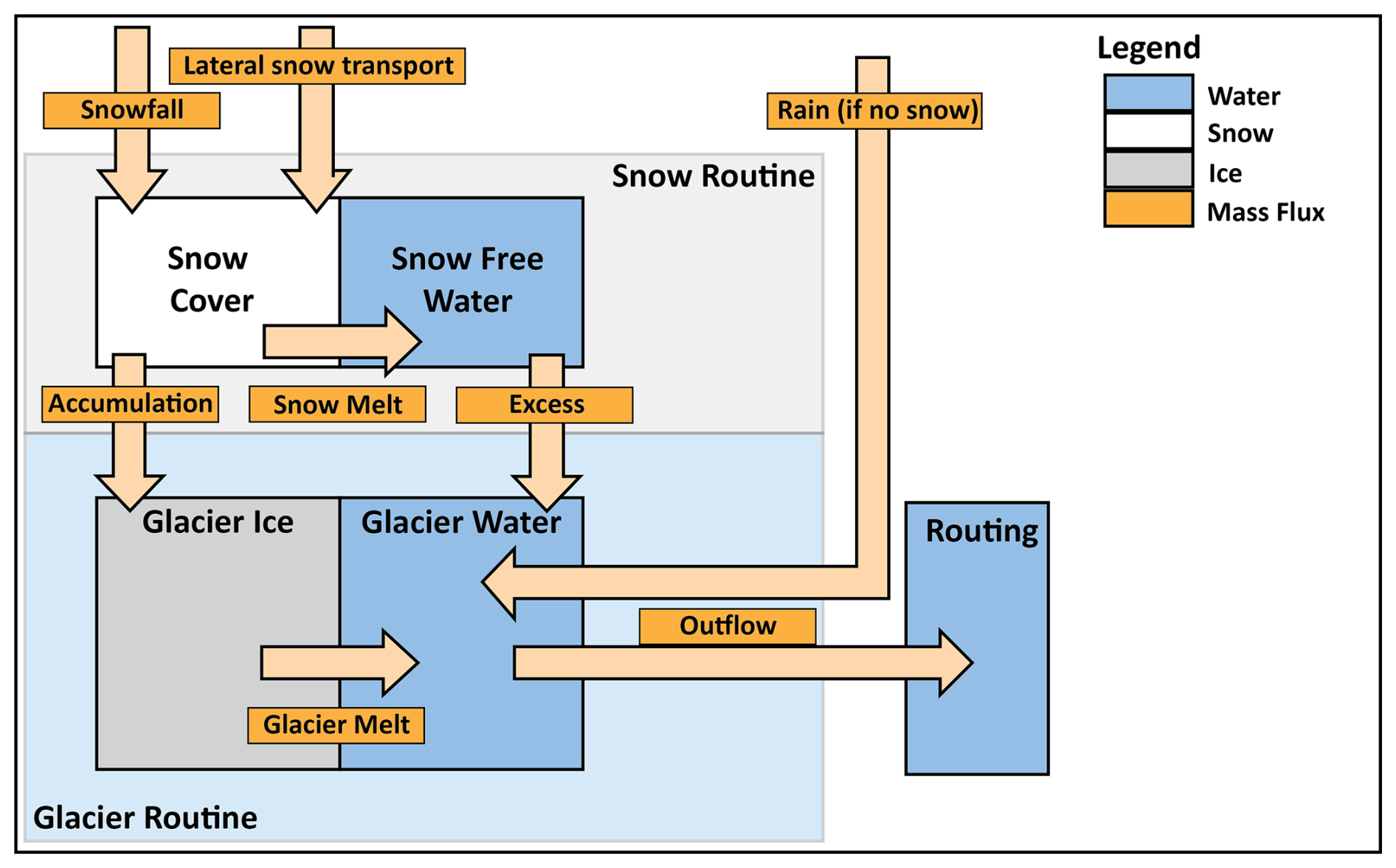
The static part of the glacier scheme is based on Seibert et al. (2018a) and is schematically shown in Fig. 3. The glacier consists of two parts, namely an ice reservoir and a water reservoir, representing water contained within the glacier. The glacier ice reservoir only decreases by melting when it is not covered by snow, following a simple temperature index scheme (see Eq. 1) using the DDF for snow multiplied with a correction factor (C_ice) to account for the lower albedo of the glacier ice surface (Seibert et al., 2018a). The glacier water reservoir increases in volume through the addition of glacier melt, snowmelt occurring on the glacier, and rain falling on the glacier during times when no snow is present. If snow cover is present, rainfall is added to the snow free water reservoir. The glacier water is then released from each individual glacier cell in the following way (Stahl et al., 2008):

$$\begin{array}{}\text{(5)}& Q=S(K_{\text{min}}+K_{\text{range}}\cdot e^{-A_{\text{g}}\text{SWE}}),\end{array}$$

where Q is the glacial water release (m d⁻¹), S is the glacial water storage (m), and SWE is the snow water equivalent in the glacier cell (m). K_min, K_range (d⁻¹), and A_g (m⁻¹) are additional parameters determining the rate of meltwater release.

For glacier accumulation, everyday, a fraction (f_acc; d⁻¹) of the snow on the glaciers is converted into glacial ice and is added to the glacier ice reservoir (Seibert et al., 2018a).

Glacier geometries change over time depending on their mass balance, which affects the quantity of melt over time. To account for such temporal changes, we implement the empirical Δh-parameterization scheme from Huss et al. (2010), as implemented in HBV (Seibert et al., 2018a). As the glacier volumes are representative of approximately the year 2003, we only apply this scheme after the year 2000, keeping the glacier volume and area constant between 1990–2000 while still calculating ice melt and accumulation. The Δh parameterization is based on the assumption that glacier mass loss leads to specific patterns of change in glacier ice surface elevation. Huss et al. (2010) identified specific parameterizations for glaciers of different sizes that relate changes in mass to surface elevation changes. Note that we do not apply the width scaling applied by Seibert et al. (2018a) as we are running the model in a spatially distributed way. Before running the model, we assign a glacier ID to each group of glacier cells that are part of an individual glacier based on the RGI outlines. Then, we create offline maps of distributed glacier thickness, where each individual glacier loses a specific fraction of its mass (in steps of 1 % mass loss) following Seibert et al. (2018a). During the hydrological model runs, we update the individual glacier geometries each year after 1 September (i.e. beginning of the hydrological year as used by the OSHD) by reading the distributed glacier thickness from these offline maps based on the mass balance simulated for the current year. Mass changes do not necessarily occur in steps of 1 %, leading to leftover mass or mass loss: for example, if the total mass loss of a glacier is 2.3 % of the initial volume, we are left with 0.3 % of leftover mass loss for this glacier. To address this, we distribute such leftover mass or mass loss evenly over the glacier area. Under the Δh parameterization, glaciers can only grow to their original extent. If glaciers gain mass compared to their initial extent, we add the additional mass to the grid cell downstream of the glacier. A full description of the Δh parameterization is provided in Appendix B.

2.3.3 Soil module

In the original model setup, each grid cell in PCR-GLOBWB 2.0 has two main soil layers and can contribute to river flow in three main ways: via direct runoff (infiltration or saturation excess), interflow, or groundwater contributions (Sutanudjaja et al., 2018). The first two components can be considered to be “fast” components, whereas the latter represents a “slow” component. Initial model runs performed with this standard setup suggested that the model produces too-slow runoff responses and cannot properly represent the fast components. Therefore, we introduced some measures to allow the model to produce more flashy runoff responses. Based on a sensitivity analysis, we decided to reduce the size of the top soil layer by making it half as thick everywhere while keeping the total soil thickness constant. Since the depth of the upper soil layer in PCR-GLOBWB 2.0 is constant over the domain and is by default set to 30 cm (Bierkens and Van Beek, 2009), halving the thickness still corresponds to a thickness of 15 cm, which is in line with the range of thicknesses that other LHMs are able to resolve (Telteu et al., 2021). This simple change should better represent the behaviour of thin soils often found on steep slopes (Weingartner et al., 2003) and causes saturation excess and interflow to occur more rapidly, thus enabling faster runoff responses.

2.3.4 Calibration

PCR-GLOBWB 2.0 has not been calibrated and generally uses parameters derived from external datasets (Sutanudjaja et al., 2018). Still, we do calibrate the degree-day factors of snow and ice to increase regional applicability and to ensure realistic glacier geometry evolution. We calibrate based on the specific process (e.g. SWE) instead of discharge to avoid compensating for deficiencies in other processes with parameter calibration and to increase the stability of these parameters when temperatures change (Sleziak et al., 2020). We try to find one parameter set that is regionally valid, i.e. constant over the entire domain. To save computational time, we perform the calibration of snow and glacier parameters offline; i.e. we run the snow and glacier component separately without running the rest of PCR-GLOBWB 2.0 and compare it to the reference datasets. We use Monte Carlo sampling as implemented in the SPOTPY Python package (Houska et al., 2015) and manually test the realism of identified parameter sets. In contrast, model evaluation is performed using the full model run. The considered calibration period is 2000–2009 (see Sect. 2.4). Note that any other parameters not mentioned here remain fixed, and their values can be found in Table S1 in the Supplement.

The updated snow module required the calibration of two parameters, namely DDF_max and DDF_min. As a reference dataset, we used a snow water equivalent reanalysis product over Switzerland (Mott et al., 2023). We chose this dataset because of its extensive data assimilation; its spatial continuity; and its high quality, which is unmet by products covering larger spatial domains (e.g. ERA5-Land or CERRA-Land), and because Switzerland covers diverse climatic regions. However, as with every other SWE dataset, this product also comes with some uncertainties. Note that we do not calibrate over Austria – even though we have similar data available there as well – to be able to test the transferability of the snow scheme to other regions. To explicitly account for elevation-dependent melt patterns, we averaged SWE spatially over partially overlapping elevation zones (500–1500, 1000–2000, 1500–2500, 2000–3000, 2500–3500 m, and Switzerland) and maximized the average Nash–Sutcliffe efficiency (NSE; Nash and Sutcliffe, 1970) across these elevation bands.

After the snow calibration, we calibrate the glacier module. This module requires the calibration of a melt correction factor C_ice and accumulation factor f_acc. We use satellite measurements of glacier elevation changes (Hugonnet et al., 2021a) as a reference dataset due to their coverage of all glaciers in the calibration domain (Switzerland for consistency with the snow calibration). We calculate the elevation changes between the beginning and end of the calibration period: we correct the model output for density differences between ice and water (ρ_ice=916.7 kg m⁻³; ρ_water=1000 kg m⁻³), only focus on locations with larger elevation changes (>2 m) to avoid noise), and minimize the mean absolute error for the elevation changes.

2.4 Evaluation

The aim of our evaluation is to assess the effect of the model development both on simulated discharge and the representation of individual processes such as snow accumulation and snowmelt. We thus evaluate the forcing datasets for precipitation and the model output for streamflow, SWE, glacier mass balance changes, glacier surface elevation evolution, and soil moisture. We generally evaluate the daily simulations, except for the glaciers for which we use annual mass balances. For the evaluation, we split the study period into three blocks with different annual mean air temperature characteristics: (1) the calibration period (2000–2009), (2) a colder evaluation period (evaluation I, 1990–1999), and (3) a warmer evaluation period (evaluation II, 2010–2019) (see Fig. S1a in the Supplement). The main evaluation is performed over evaluation II, which is also the period considered if a specific time interval is not specified. In the Supplement (Sect. S2), we use both evaluation periods to assess the transferability of the new model setup to time periods with different mean temperatures within the framework of a differential split sample test (DSST; Klemeš, 1986; Seibert, 2003).

The evaluation of the meteorological forcing focuses on precipitation, which is more spatially heterogeneous than temperature. We try to analyse the differences between the datasets and their realism, acknowledging the large uncertainties around high-altitude precipitation. We resample all three forcing datasets (STANDARD, CHELSA, and CERRA; see Sect. 2.2) to the grid points of the coarser reference APGD and calculate both the Pearson correlation and the absolute bias against the APGD.

We evaluate the performance of the daily discharge simulations by comparing simulated discharge against observed streamflow, i.e. the station data from the LHDA+. We match model grid cells to discharge stations by matching the catchment contours following Godet et al. (2024). We then evaluate discharge simulation performance by comparing the simulated time series to the observed time series using the Kling–Gupta efficiency (KGE; Gupta et al., 2009), using only stations that have at least 3 years of data over the considered evaluation period (number of valid stations: evaluation I – 1676, calibration period – 1869, evaluation II – 2105). The KGE is defined as follows:

$$\begin{array}{}\text{(6)}& \text{KGE}=\mathrm{1}-\sqrt{(r-\mathrm{1}{)}^{\mathrm{2}}+{\left({\displaystyle \frac{{\mathit{\mu }}_{\mathrm{sim}}}{{\mathit{\mu }}_{\mathrm{obs}}}}-\mathrm{1}\right)}^{\mathrm{2}}+{\left({\displaystyle \frac{{\mathit{\sigma }}_{\mathrm{sim}}}{{\mathit{\sigma }}_{\mathrm{obs}}}}-\mathrm{1}\right)}^{\mathrm{2}}},\end{array}$$

where r is the Pearson correlation coefficient between observations and simulations, μ_obs is the mean over the observations, μ_sim is the mean over the simulations, σ_obs is the standard deviation over the observations, and σ_sim is the standard deviation over the simulations. KGE scores above −0.41 indicate that model simulations improve performance compared to assuming a constant flow corresponding to the average of the observed discharge time series (Knoben et al., 2019). To assess whether and by how much a specific change in model structure improves model performance for discharge, we use the KGE skill score (KGESS) as used by Knoben et al. (2020) and Van Jaarsveld et al. (2025). The KGESS compares the KGE score of a model run with a new setup against a model benchmark:

$$\begin{array}{}\text{(7)}& \text{KGESS}={\displaystyle \frac{{\text{KGE}}_{\text{model}}-{\text{KGE}}_{\text{bench}}}{\mathrm{1}-{\text{KGE}}_{\text{bench}}}},\end{array}$$

where KGE_model is the KGE score of the new model run, and KGE_bench is the KGE score of a benchmark model run, which represents an intermediate step within the model improvement chain.

The Alpine region contains many reservoirs for water regulation, especially for hydropower production (Lehner et al., 2005; Brunner and Naveau, 2023). Their presence and how they are represented can influence model performance (e.g. Hanasaki et al., 2006; Abeshu et al., 2023). Therefore, we investigate how model performance for discharge varies between natural and regulated catchments. As not each catchment with a reservoir might be strongly regulated, we define a catchment's degree of regulation by dividing its total reservoir capacity by its mean discharge (in units of time). We only consider a catchment to be regulated when this degree of regulation exceeds 0.1 years (see Fig. S3 in the Supplement). Another way to separate regulated from natural catchments is the water balance signature (WB), which describes the normalized deviation from a closed water balance assuming no long-term storage effects (Salwey et al., 2023). WB is defined as follows:

$$\begin{array}{}\text{(8)}& \text{WB}={\displaystyle \frac{Q}{P}}-\left(\mathrm{1}-{\displaystyle \frac{E_{\text{P}}}{P}}\right),\end{array}$$

where Q is the (observed) averaged discharge (mm d⁻¹), P is the precipitation (mm d⁻¹), and E_P is the potential evapotranspiration (mm d⁻¹) averaged over the catchment and study period. Positive values of WB indicate that a catchment's discharge is higher than expected. Assuming that the meteorological components could be well-estimated, such positive values could suggest that a catchment gains more water than what comes in through precipitation. Negative values of WB indicate that a catchment loses more water than just the potential evapotranspiration. Salwey et al. (2023) have shown that this metric can be used to identify catchments affected by hydropower production and water transfers. In addition, we performed a small evaluation which indicated that, indeed, there exists a relationship between WB and the degree of regulation (see Fig. S3 in the Supplement). However, other factors such as errors in the meteorological forcing or additional water input from glaciers due to imbalance can also lead to strong water balance deviations, which can also affect model performance with respect to discharge. We thus use WB as a general metric to study the effect of such deviations in the water balance on model performance. Furthermore, we also use WB as an indication of water transfers, hydropower production, and other water balance deviations in combination with catchment-based information on reservoirs.

In addition to discharge, we evaluate model performance for SWE by calculating spatial averages over different elevation bands (0–1000, 1000–2000, 2000–3000 m, or the entire country) over Switzerland. Additionally, we evaluate it over Austria, which has not been used for model calibration and can therefore provide insights into how well the model generalizes to other regions. Then, we compute the average seasonal SWE cycle over these zones and compare it to the seasonal SWE cycles derived from different snow reanalysis products (OSHD, SNOWGRID; see Table ). Furthermore, we calculate the KGE for SWE by comparing modelled SWE and SWE inferred from observations at specific measurement stations (NH–SWE; see Table ).

We evaluate glacier simulations in terms of both their mass balance and their geometry evolution. Simulated mass balances were summed over the hydrological year (starting in October to facilitate comparisons with the observations of WGMS and GLAMOS; see Table ) and compared to observed time series, as well as to observed average geodetic mass loss estimates derived from GECM. To evaluate glacier geometry evolution, we both visually compare spatial patterns of glacier surface elevation changes against observations (GECM; see Table ) and quantitatively evaluate long-term glacier changes. It is difficult to evaluate the long-term response of simulated glaciers to climate forcing given the relatively short study period. To address this problem, we repeat an experiment by Zekollari et al. (2020), in which glaciers are continuously forced (for 300 years) with the modelled mean mass balance for the period before 2018. The glaciers respond to this forcing by changing their shapes, and they stabilize when they are in balance with the applied forcing. We then compare this to the estimates of Zekollari et al. (2020).

We evaluate soil moisture against the ESACCI soil moisture dataset. This evaluation is more difficult than the evaluation of other variables since the satellite data are not directly comparable to our model output: they measure soil moisture in the top 5 cm of the soil, whereas we model moisture in the top 15 or 30 cm (see Table ). Furthermore, the resolution of the observations is much coarser than the one of the simulations. Therefore, we resample our simulations to the resolution of the satellite data using spatial averages and only select locations with at least 50 % of valid daily data over evaluation II. We calculate the Spearman rank correlation coefficient between the daily model simulations and the satellite observations to assess model performance because this metric should be applicable despite the different soil moisture depths.

3 Results

3.1 Effect of meteorological forcing

Precipitation in all three meteorological forcing datasets used in this comparison correlates well with gridded precipitation station data from the APGD (see Fig. 4). Precipitation from CERRA-CHELSA shows generally higher correlations with observed precipitation than the precipitation of the STANDARD and CHELSA input datasets (compare Fig. 4a and b with c). The correlation between the three datasets and the reference dataset varies across the Alps and is especially low in the Po Plain. All meteorological datasets show a positive bias in precipitation over the Alps and a negative bias over the Apennines (see Fig. 4d, e, and f). Around the Alps, the STANDARD and CHELSA forcings show slightly positive biases, whereas CERRA-CHELSA shows a slightly negative bias. Overall, CERRA-CHELSA and STANDARD have a smaller precipitation bias than the CHELSA dataset (mean absolute bias: CERRA-CHELSA – 0.4 mm d⁻¹, CHELSA – 0.5 mm d⁻¹, STANDARD – 4 mm d⁻¹).

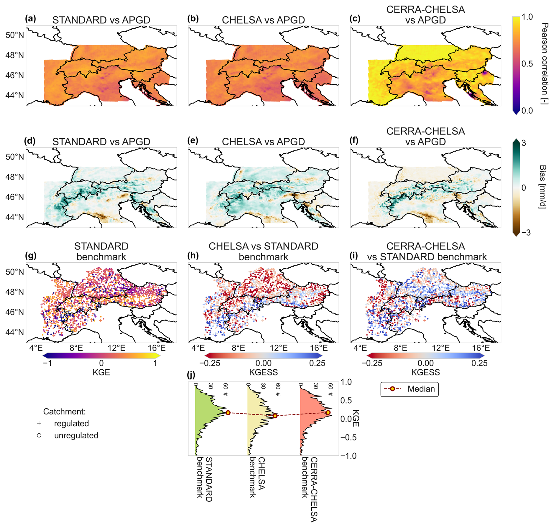
Figure 4 Differences in meteorological forcing datasets and the effect of their choice on model performance for discharge over the larger Alpine domain. Panels (a)–(c) compare the correlation of precipitation in the (a) STANDARD, (b) CHELSA, and (c) CERRA-CHELSA datasets with observed precipitation (APGD, 2000–2008). Panels (d)–(f) show the bias of mean daily precipitation against observed precipitation for the (d) STANDARD, (e) CHELSA, and (f) CERRA-CHELSA datasets. Panels (g)–(i) compare discharge simulations generated with the different forcing datasets – (g) KGEs for the STANDARD benchmark run, (h) KGESS for the CHELSA benchmark run, and (i) the CERRA-CHELSA benchmark run – against the STANDARD benchmark run. (j) Ridge line plots showing the distribution of KGEs (in number of catchments) for the three benchmark runs. Note that roughly 6 % of the stations have a KGE smaller than −1 and fall outside of the bounds in (j).

The choice of meteorological forcing has a strong effect on simulated discharge, but the effect is not uniform across catchments. Using the STANDARD forcing, we see generally better model performance for discharge over the Alps than in the surrounding areas (see Fig. 4g). However, locally, there is poor model performance for discharge in certain catchments in the western Alps, southern Switzerland, and eastern Austria. Forcing the model with CERRA-CHELSA leads to improved performance in these regions, as well as in southern Germany (see Fig. 4i). In contrast, CERRA-CHELSA leads to reductions in model performance for discharge in eastern France, parts of Switzerland, and western Austria. Using CHELSA leads to a slight worsening of model performance for discharge compared to runs with STANDARD or CERRA-CHELSA forcing, except in parts of the Alps (see Fig. 4h).

In summary, we find that discharge simulations generated with the CERRA-CHELSA and STANDARD forcing datasets are generally better than those generated with the CHELSA dataset (see Fig. 4j). As the precipitation of the CERRA-CHELSA dataset aligns better with the reference precipitation dataset than the STANDARD dataset (see Fig. 4a, b, d, and e), we performed all further analyses with the CERRA-CHELSA dataset.

3.2 Snow representation

SWE representation benefits to some degree from the proposed adjustments in the snow module (see Fig. 5). The introduction of the snow transport scheme only improved snow representation at the highest elevations (2000–3000 m), where unrealistic snow towers were a major issue (compare the transport run with the CERRA-CHELSA benchmark run in Fig. 5c and f). Here, the snow transport scheme ensures that the snow is redistributed to lower elevations, where it subsequently melts away. ERA5-Land and CERRA-Land also show very high SWE values, suggesting that these models also suffer from unrealistic snow build-up. Without calibration, further structural changes to the snow module (i.e. the seasonally varying DDF, exponential temperature dependence, and a rain-to-snowfall transition temperature range) did not improve performance against observational SWE stations (see Fig. 5g and h). Averaged over elevation zones, however, these changes lead to an improvement in the SWE representation at higher elevations (e.g. for elevation zone 2000–3000 m, the KGE compared to the reference products increases from 0.85 to 0.89 over Switzerland and from 0.53 to 0.57 over Austria). At lower elevations, these changes lead to too-low melt rates over Austria (for elevation zone 1000–2000 m, KGE increased from 0.87 to 0.88 over Switzerland but dropped sharply from 0.64 to 0.46 over Austria; compare uncalibrated snow and transport runs in Fig. 5a, b, d, and e). These differences between elevation zones suggest that the model structure leads to varying melt rates with elevation: this is to be expected as the temperatures at which snow starts to melt are reached later in the year at higher elevations, such that the same temperatures are combined with different values of the time-varying DDF which produces differing melt rates. Calibrating the DDF in the snow module against SWE shows the best performance over Switzerland (KGE averaged over Switzerland against OSHD: 0.91), though still with slightly too-high melt rates over Switzerland (see full model run in Fig. 5a, b, and c). In Austria, the calibrated snow run is, while slightly less accurate than in Switzerland, the most accurate of the presented model runs (KGE averaged over Austria against SNOWGRID: 0.80), even though no Austrian SWE data were used for calibration (see Fig. 5d, e, and f). This demonstrates that the snow module is generally transferable to other regions. The comparison of our model runs against SWE estimates at measurement stations (see Fig. 5g and h) confirms that SWE simulations profit from the calibration.

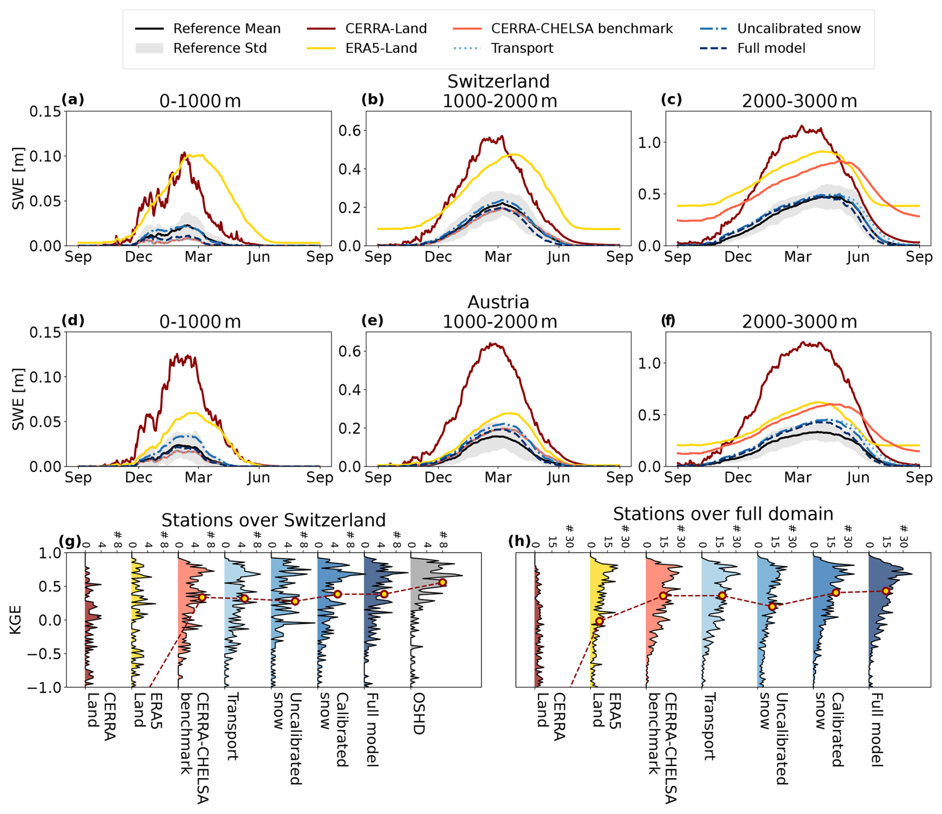
Figure 5 Snow representation for different elevation zones and regions. Average snow climatology over Switzerland (a–c) and Austria (d–f) for grid cells at elevations between 0–1000 m (a, d), 1000–2000 m (b, e), and 2000–3000 m (c, f) derived from the gridded simulations and reanalysis products. The reference products are the OSHD reanalysis for Switzerland and the SNOWGRID product for Austria. Note that, for simplicity, we only show the full model run instead of the calibrated snow run as these have the same snow module configuration. Panels (g) and (h) show KGEs of SWE time series at the different measurement stations of Fontrodona-Bach et al. (2023b) over Switzerland (g; 251 stations) and the full Alpine domain (h; 1047 stations) for different model runs and reanalysis products. For (g) and (h), note that roughly 3 % to 10 % of stations have a KGE < −1 (>30 % for CERRA-Land and ERA5-Land).

Changes in SWE performance are reflected in the performance of discharge simulations (see Fig. 6). Snow transport improves discharge simulations in the highest parts of the Alps but has hardly any effect outside of the mountains (see Fig. 6b). Structural changes to the snow module lead to an improvement in discharge simulations in catchments at the highest elevations but a worsening in catchments at lower elevations (see Fig. 6c). Finally, calibrating SWE improves discharge representation in most of the catchments that worsened from the structural changes, with a few exceptions in the Alps (see Fig. 6d). Figure 7a, b, and c illustrate that the changes in the snow module mainly improve model performance for discharge in catchments with high snowfall fractions, whereas the changes are negligible or slightly negative in catchments with low snowfall fractions. Still, some catchments with high snowfall fractions experience decreases in performance for discharge: these decreases mostly happen in the presence of reservoirs and/or with negative values of WB (median KGESS for catchments with more than 30 % snowfall compared to CERRA benchmark: regulated 0.017, unregulated 0.080).

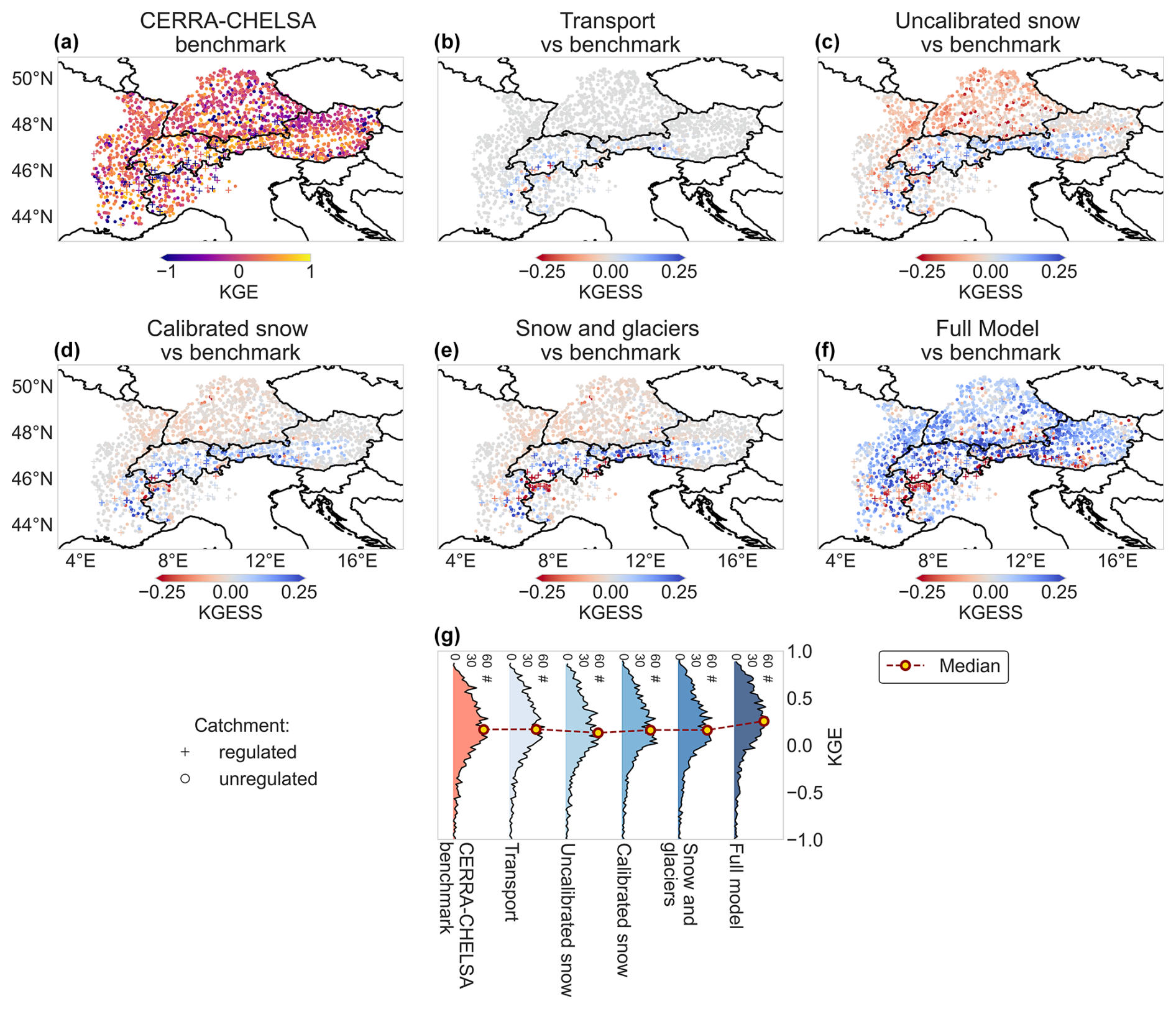
Figure 6 Model performance and its changes in terms of discharge at the measurement stations for different adjustments in the snow routine. (a) Absolute KGEs for the CERRA-CHELSA benchmark run. Changes in performance (KGESS) with respect to the CERRA-CHELSA benchmark run for different model configurations: (b) transport, (c) uncalibrated snow, (d) calibrated snow, (e) snow and glacier, and (f) full model (including soil thickness change). (g) Distribution of KGE scores for the different model runs across catchments. Note that roughly 6 % of stations have a KGE smaller than −1 and fall outside of the bounds.

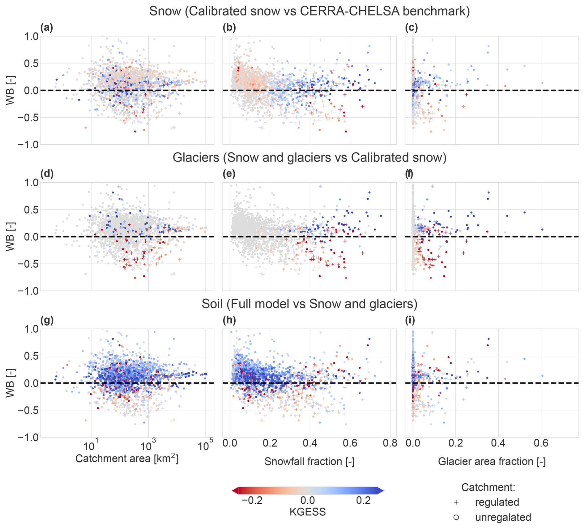
Figure 7 Model performance change for discharge (KGESS) at the measurement stations after introducing different adjustments into the model (indicated with the colours). The model performance changes are compared to catchment characteristics. (a–c) Effect of the combined snow changes on discharge simulations (difference between the calibrated snow and the CERRA-CHELSA benchmark runs), (d–f) effect of the introduction of glaciers (snow and glaciers vs. calibrated snow), and (g–i) effect of the changes made to the soil (full model vs. snow and glaciers). Panels (a), (d), and (g) show the dependence of model performance changes for discharge on WB and catchment area; (b), (e), and (h) show the dependence on WB and snowfall fraction; and (c), (f), and (i) show the dependence on WB and glacier area fraction. Note that roughly 3 % of the stations have a WB larger than 1 and fall outside of the figure bounds.

3.3 Glacier representation

The new glacier module captures the general behaviour of glaciers. Both spatial patterns of glacier elevation changes and time mean patters of mass balances are roughly reproduced (see Fig. 8a, b, c, d, e, and f), even though the model shows biases for individual glaciers in terms of mass balance (see Fig. 8a, b, and g) or retreat (see rapid retreat of Mer de Glace in Fig. 8d). Generally, mean geodetic mass balances are underestimated (see Fig. 8g). Figure 8h shows the results from the equilibrium experiment based on Zekollari et al. (2020). Most glaciers reach equilibrium over time, although there is significant committed mass loss. Overall, we end up with around 40 % committed mass loss in 2018, which was also found by Zekollari et al. (2020). Our modelling scheme thus captures the general behaviour of long-term glacier responses, with glacier retreat adjusting to a new steady-state condition. However, we see deviations for individual glaciers, with a larger glaciers generally retreating slightly less and smaller glaciers retreating slightly more than the reference dataset. In conclusion, our model evaluation shows that the new glacier module works reasonably well for the total or groups of Alpine glaciers (see Fig. 8g and h), while it can be significantly biased at the scale of individual or small glaciers (see Fig. 8g, h).

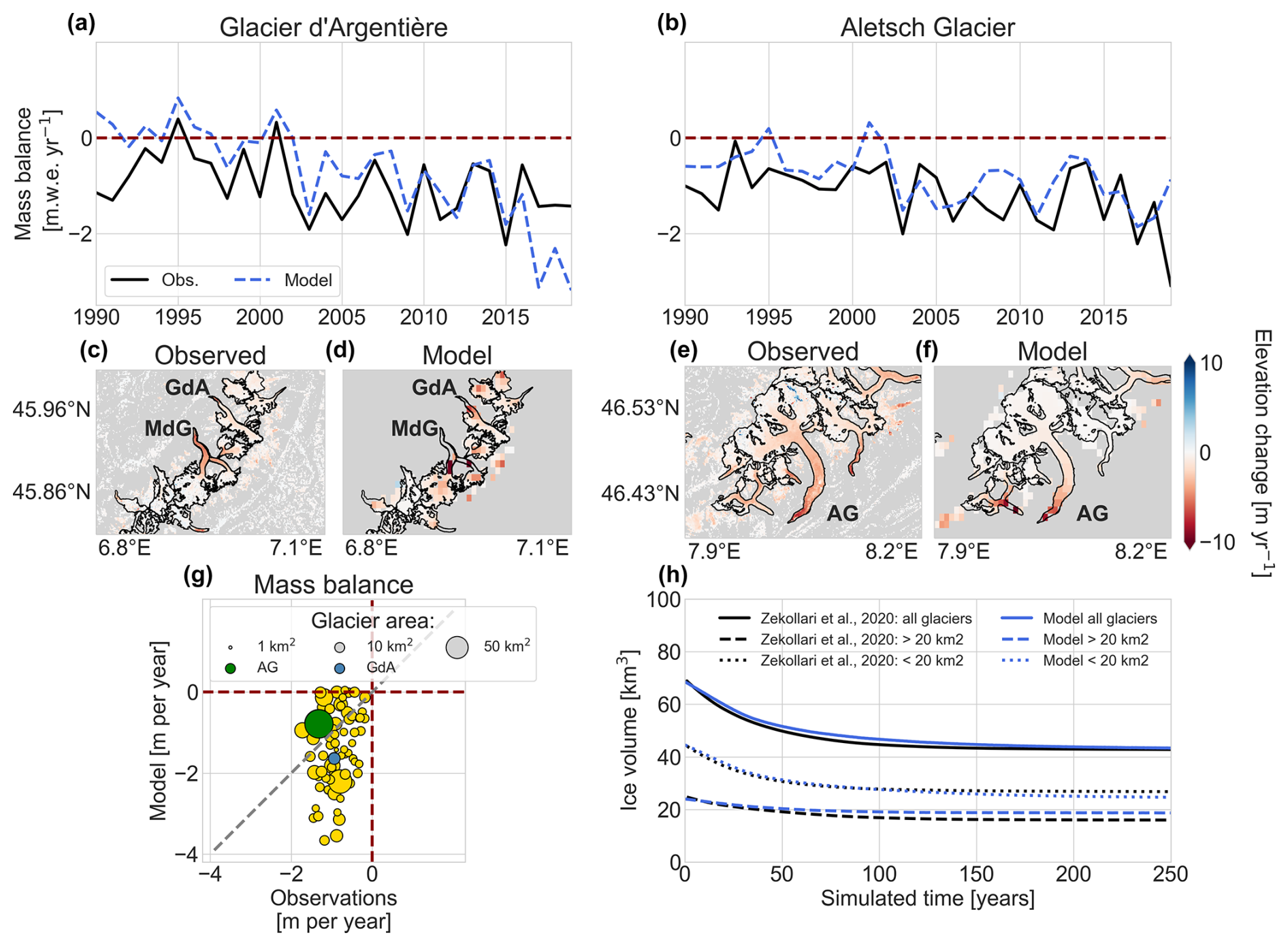
Figure 8 Evaluation of the glacier scheme newly integrated into the hydrological model. Panels (a) and (b) show annual time series of simulated against observed mass balance in metres of water equivalent per year for Glacier d'Argentière (a) and Aletsch Glacier (b) (observations for Aletsch: Glacier Monitoring Switzerland (GLAMOS), 2022; Argentière: World Glacier Monitoring Service (WGMS), 2023). Panels (c) and (d) show the elevation change over 2010–2019 for the region around Glacier d'Argentière (c – observations; d – model) and around the Aletsch Glacier (e – observations; f – model). Observations are from Hugonnet et al. (2021a), and outlines are from GLIMS Consortium (2018). (g) Average elevation change (2010–2019) of glaciers against observations from Hugonnet et al. (2021a). (h) Comparison of the evolution of glacier volume over time under this continuous forcing with their mean mass balance from 1990 to 2018 to modelled estimates from Zekollari et al. (2020). AG represents Aletsch Glacier, and GdA represents Glacier d'Argentière.

The addition of the glacier module mainly improves discharge simulations in highly glacierized catchments (see Figs. 6e and 7f). The positive effect of glaciers is much less visible in catchments with a small glacier or snowfall fraction (see Fig. 7e). Furthermore, our results indicate that, in certain regions, especially around the heavily regulated Rhône River in southwestern Switzerland, discharge performance can decrease with the addition of glaciers (see Fig. 6e). Such a performance decrease generally occurs in catchments with a negative WB or reservoir regulation (see Fig. 7f; median KGESS in catchments with >5 % glacier cover compared to calibrated snow: regulated −0.19, unregulated 0.15).

3.4 Soil partitioning

Model performance for soil moisture varies over the domain (see Fig. 9a and b), with generally higher performance in flatter low-elevation areas (such as the Rhone Valley, the Po Plain, or the Rhine Valley) and lower performance over hilly or mountain areas. Implementing the soil changes has a mixed effect on performance: generally, it improves performance in areas where the model was already performing well (i.e. the lower flatlands) and worsens performance in locations with lower model performance (see Fig. 9c).

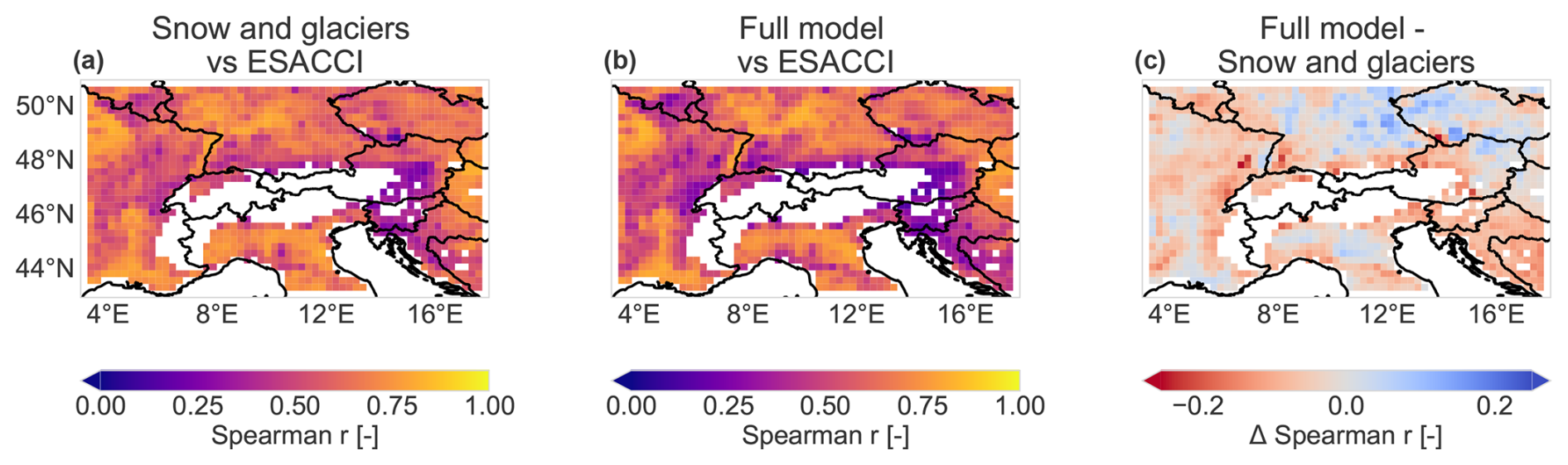
Figure 9 Comparison of soil moisture simulations against the ESACCI satellite observations. We show the Spearman correlation between the snow and glacier (a) and full model runs (b) against the ESACCI observations. (c) Difference in Spearman correlation coefficients between the full model and the snow and glacier runs. White areas indicate regions which had too many days without data (more than 50 % of the time).

Over the entire domain, the changes made to the soil module, i.e. to the runoff partitioning, generally increase model performance for discharge (see Fig. 6f). The improvements in discharge performance are strongest in catchments with lower snowfall fractions (<0.3; see Fig. 7h) and are generally independent of the catchment area (see Fig. 7g). Discharge performance increases are stronger in unregulated catchments (see Fig. 7g, h, and i; median KGESS compared to snow and glaciers: regulated 0.03, unregulated 0.09).

3.5 Evaluation of new model setup

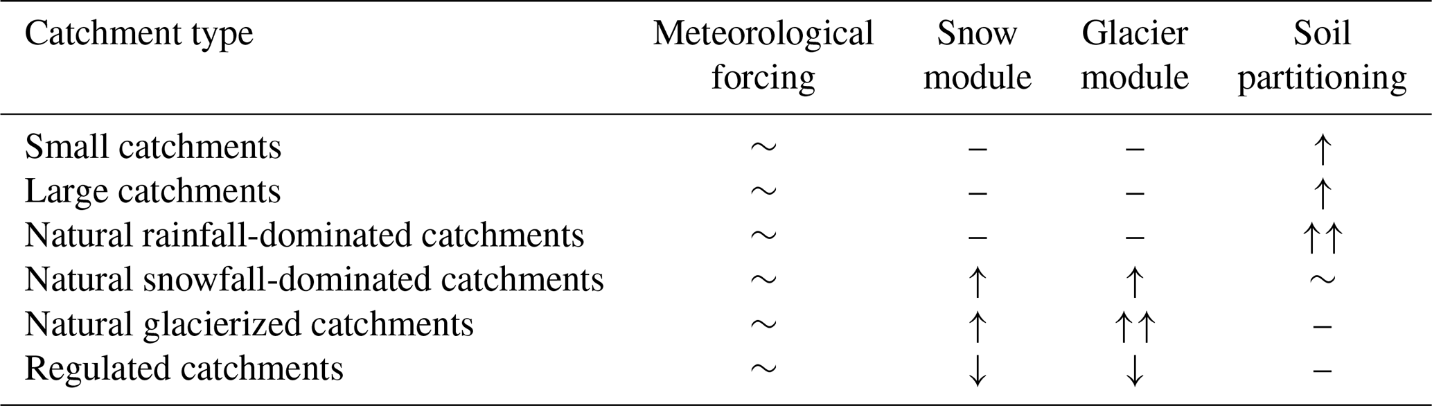
Our new model setup, which includes updated snow, glacier, and soil modules, leads to general performance increases in streamflow simulations compared to the existing PCR-GLOBWB 2.0 setup, with performance depending on catchment characteristics (see Fig. 10 and the summary provided in Table 3 and Fig. 11). Catchment area and WB are major controls of absolute model performance for discharge in terms of KGE, which is highest in large and natural catchments, in which the water balance is nearly closed (see Fig. 10a). Similarly, the model performs well in snow-covered and glacierized catchments, where the model additions lead to a substantial improvement in model performance for discharge (see Fig. 10b, c, e, and f). In contrast, the model adjustments can decrease performance in catchments with a negative WB (see Fig. 10d, e, and f; median KGESS of full model against CERRA benchmark: positive WB 0.09, negative WB 0.02).

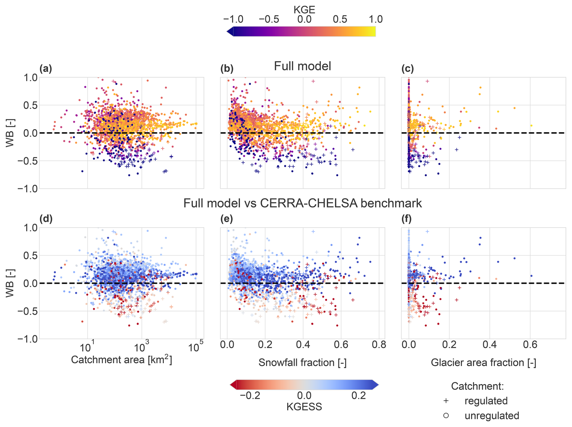
Figure 10 Model performance of the full model run for discharge (a–c, showing KGE) and the total model performance changes for discharge compared to the CERRA-CHELSA benchmark run (d–f, showing KGESS) in the evaluation catchments in relation to different catchment characteristics: WB and catchment area (a, d), WB and snowfall fraction (b, e), and WB and glacier area fraction (c, f). Note that roughly 3 % of the stations have a WB larger than 1 and fall outside of the figure bounds.

Table 3 Summary of the effect of the different model implementations on discharge simulations. The symbols have the following meaning: ↑ denotes improvement, $\uparrow \uparrow$ denotes large improvement, ↓ denotes worsening, $\downarrow \downarrow$ denotes large worsening, – denotes no effect, and ∼ denotes substantial but mixed effect.

4 Discussion

4.1 Evaluation and recommendations for further model development

Our new model setup generally led to increased model performance compared to the old setup: structural and parameter changes applied to the snow, glacier, and soil modules improved both SWE and discharge simulations (Figs. 6, 7, 5, and 10). This highlights the importance of improving process representation in hyper-resolution modelling efforts.

Updating the runoff partitioning in the soil leads to a clear improvement in the simulation of discharge in natural catchments (Figs. 6f and 7g, h, and i; column “soil partitioning” in Table 3), with rainfall-dominated catchments (≈ less than 30 % snowfall) benefiting the most (Fig. 7g and h). This major increase in model performance is caused by a modest change in the soil parameters, supporting the suggestion that the move to a hyper-resolution requires careful review of parameterizations in LHMs (Hoch et al., 2023). Still, absolute performance in smaller rainfall-dominated catchments remains relatively limited (Fig. 10a and b). In addition, soil moisture representation did not improve in regions that already had poor performance (Fig. 9c and d). Please note that the reference product used for computing model errors can have its own biases (Dorigo et al., 2015, 2017) and has a much coarser spatial resolution than our model, and so error estimates might not be entirely representative. Our results therefore suggest that there is a need for more representative ways to compare soil moisture simulations and observations. Still, the representation of soil moisture and fast discharge responses needs to be further improved if LHMs are to be applicable at smaller spatial scales. These further improvements can come from two directions: first, soil heterogeneity could be included in models in more detail. For example, Van Jaarsveld et al. (2025) suggested that sub-grid-scale land cover variability could still be important in hyper-resolution modelling, and we hypothesize that this would also improve the representation of spatial variations in discharge behaviour. However, including this information would come at the cost of increased computational demands. Second, more explicit consideration of hillslope processes such as preferential flow in the model structure (e.g. Rahman and Rosolem, 2017; Gharari et al., 2019; Fan et al., 2019) could lead to further improvements in the simulation of flashy runoff responses.

Discharge simulations mostly benefit from the structural changes made to the snow module in snow-dominated catchments (Figs. 6c and 7e; column “snow module” in Table 3). Similarly, Girons Lopez et al. (2020) found, for the catchment model HBV, that exponential melt combined with seasonally varying DDFs improved discharge simulations, whereas the rain-to-snow transitions improved SWE representation but led to slightly poorer results for discharge. However, whereas our discharge simulations in most snow-dominated mountain catchments improved due to these structural changes, we noted a slight decrease in discharge performance at lower elevations, where snow contributions are less important. One reason for why the structural changes in the snow module are better suited for catchments in mountainous terrain might be differences in terms of the dominant snow processes between high and low elevations, such as the frequency of rain-on-snow events. Since Magnusson et al. (2014) built their snow model for alpine Switzerland, they might have prioritized representing melt patterns at higher elevations with thick snow cover over patterns in flatter terrain with only limited snowfall. For example, our scheme does not explicitly include melt due to liquid precipitation. Another reason for this slight decrease in discharge performance at lower elevations could be related to our choice of regionally averaged DDFs since, in reality, these DDFs show smaller-scale variability in space (e.g. with aspect, albedo, elevation, land cover, and vegetation) (e.g. Kuusisto, 1980; Rango and Martinec, 1995; Hock, 2003; Ismail et al., 2023). Such variability is not accounted for in our model since we focused on regionally valid parameterizations instead of local solutions. However, ignoring this variability could lead to biases in SWE representation in specific locations. More elaborate snow module formulations, such as parameterizations that include aspect (e.g. Immerzeel et al., 2012) or radiation (e.g. Hock, 1999), could increase our ability to capture more detailed spatial melt patterns. Such approaches can become feasible now that higher spatial resolutions can resolve slopes and represent vegetation cover and land use in a more detailed way. However, they come at the cost of increased model complexity and a larger number of input variables. In any case, the slight decrease in discharge performance at lower elevations was reduced via the calibration of modelled SWE against a regional SWE reanalysis product, leaving us with a good overall discharge and SWE simulation performance (compare Fig. 6c and d). The improved discharge representation after calibration highlights the performance gains that can be achieved by including more regional data in LHMs. However, regional calibration is only possible due to the comparably high quality of observational and reanalysis data in Switzerland. Many other regions around the globe continue to face a lack of observations of water balance components (Wilby, 2019), which challenges accurate regional calibration. Furthermore, the slightly reduced performance in SWE representation over Austria (which was excluded from calibration) compared to Switzerland already indicates that parameters can vary between regions (compare Fig. 5d, e, and f with Fig. 5a, b, and c). Highly detailed calibration in one region might give a false sense of accuracy when applying the setup outside of the calibration region. Regionally valid datasets must thus be chosen with care.

Adding a glacier module led to general improvements in discharge simulations in glacierized catchments in the Alps in catchments with a near-zero or positive value for WB (i.e. more observed discharge than is “expected”; see Fig. 7f and column “glacier module” in Table 3). The effect of glaciers on general discharge performance further downstream remains limited (see Fig. 6e), although this effect might be larger during certain months or seasons (Wiersma et al., 2022). Aside from discharge, glacier mass balances and spatial patterns in elevation changes are also reasonably well represented (see Fig. 8). Still, we note that glaciers can show significant biases in the mass balance (see Fig. 8g) and in the responses (see Fig. 8j). Differences in long-term responses compared to previous experiments into which ice dynamics were incorporated might be partly explained by the Δh parameterization, which ignores potential delays in glacier response to mass changes (Seibert et al., 2018a). Further biases in both mass balance estimates and responses are likely to be related to the relatively coarse spatial resolution of our model compared to the size of individual glaciers, which makes it more difficult to accurately describe patterns in melt or snow accumulation for small glaciers consisting of only a few grid cells. Melt representation of individual glaciers could be improved by resolving glaciers at a higher spatial resolution than the resolution simulated here, for example, by including elevation zones (Seibert et al., 2018a). Resolving glaciers at a higher spatial resolution could also lead to even more realistic glacier retreat since the Δh parameterization was originally designed for higher spatial resolutions (Huss et al., 2010) and is likely to be less accurate at the coarser 30 arcsec model grid. Further gains in glacier representation could be realized by improving glacier accumulation estimates by continuing to develop the snow component or by improving spatial melt patterns by varying the glacier DDF in space (analogously to what we suggested for snow).

While the improvements in process representation generally lead to an increase in model performance for discharge, there are regions where the performance of discharge simulations decreases after implementing the structural and parametric changes (see Fig. 10d, e, and f). Our analysis shows that such performance decreases are common in catchments with negative values of WB, which can be related to issues with the meteorological forcing, glacier melt estimates, or the representation of water abstractions or (hydropower) reservoirs in the model. Indeed, the strongest negative performance changes after the introduction of snow and glaciers often occur in catchments with negative WB or regulation (see Fig. 7b and f; row “regulated catchments” in Table 3). In the Alps, significant glacier or snowmelt occurs above hydropower reservoirs (e.g. in Switzerland, 4 % of all hydropower is related to glacier mass loss; Schaefli et al., 2019). Hydropower severely changes flow seasonality (Arheimer et al., 2017), essentially decoupling observed streamflow from snowmelt and ice melt. Accurate representation of river regulation and hydropower reservoirs is thus important, but LHMs appear to have difficulties with modelling streamflow in these regulated catchments (e.g. Veldkamp et al., 2018; Tu et al., 2024). These issues might become even more apparent at a hyper-resolution because (a) small rivers are now represented and might be affected by reservoirs that are not represented in the model, and (b) reservoir schemes in LHMs were developed to represent regulation behaviour on a coarse grid (e.g. they mimic the combined effect of all reservoirs within a 50 km × 50 km grid cell) and likely need an update when moving to higher spatial resolutions (Shin et al., 2019). However, even if more reservoirs were introduced into the model, accurate discharge modelling in regulated systems remains challenging due to limited data on operation strategies and regulations (Turner and Voisin, 2022). Thus, both improving the representation of human water management in models and collecting new data should remain an active area of research.

Besides model structure and parameterization, the meteorological reanalysis forcing has a major influence on model performance for discharge (see Fig. 4g, h, and i; column “meteorological forcing” in Table 3). This implies that improvements in simulation performance that can potentially be achieved by structural changes are bound by the quality of the meteorological forcing dataset, especially in a non-calibrated model setup. Replacing the STANDARD meteorological forcing product with CERRA-CHELSA led to an overall increase in correlation with the reference dataset (compare Fig. 4a and c) but showed mixed performance changes for discharge over the model domain (compare Fig. 4g and i). This apparent inconsistency could be related to uncertainties affecting our precipitation evaluation and the LHM. Our precipitation evaluation is likely to be affected by uncertainties in the reference APGD. Although the APGD is based on a particularly dense network of direct observations, it still has uncertainties related to precipitation undercatch (for which it was not corrected) and in regions with less dense station coverage (Isotta et al., 2015). Our evaluation of the precipitation products should therefore be interpreted as an indication of consistency with interpolated surface measurements but not necessarily as an indication of absolute performance. Collecting new, better, and more observations of meteorological variables over mountainous regions should thus remain a priority. The limited performance for discharge in small flashy catchments, as was pointed out before, might further prevent the direct translation from more accurate precipitation input into improved discharge performance. The ever-present uncertainty in forcing datasets and their evaluation also highlights the advantage of the calibration strategy we proposed and applied here, which focuses on processes like snow or glaciers rather than on discharge. Calibrated models can compensate for meteorological uncertainty and model deficiencies (Refsgaard and Storm, 1996). Including the representation of processes such as snow or glaciers into the calibration procedure avoids some parameter equifinality and preserves internal relationships (e.g. Duethmann et al., 2014; Finger et al., 2015), which facilitates identifying where models need improvements. Finally, as presented in the Methods section, the STANDARD and CHELSA meteorological forcing datasets were derived using statistical or physical and/or heuristic downscaling, whereas the CERRA-CHELSA dataset is based on a dynamically generated regional reanalysis product. None of these methods used to create the hyper-resolution forcing datasets led to general improvements in simulation performance across the full domain. Regional differences between the datasets, observational uncertainty, and deficiencies in hydrological model structure did have a pronounced effect on model performance for discharge.

4.2 Applicability and limitations

Our new model setup generally shows a better representation of discharge than the existing hyper-resolution version of PCR-GLOBWB 2.0 (see Fig. 10d, e, and f). Absolute discharge performance is generally satisfactory, especially at larger spatial scales and in natural rivers (see Fig. 10a, b, and c), and spatial patterns can be resolved in high detail (see Fig. 11a and b). Applications of such hyper-resolution LHMs should thus make use of these strengths by studying spatial patterns at larger spatial scales. Still, the model shows poor discharge simulation performance in some catchments, especially in smaller catchments at lower elevations and in rivers with a negative WB. Users should thus be aware of such limitations when looking at individual catchments. While the hyper-resolution simulations might not be completely accurate in certain places, they can still be valuable in helping to complete the spatial picture and in enabling the study of spatial variability (Seibert et al., 2018b). This is especially true in regions where no observational data are available. There, these LHMs provide a first-order estimate of river discharge without requiring local calibration.

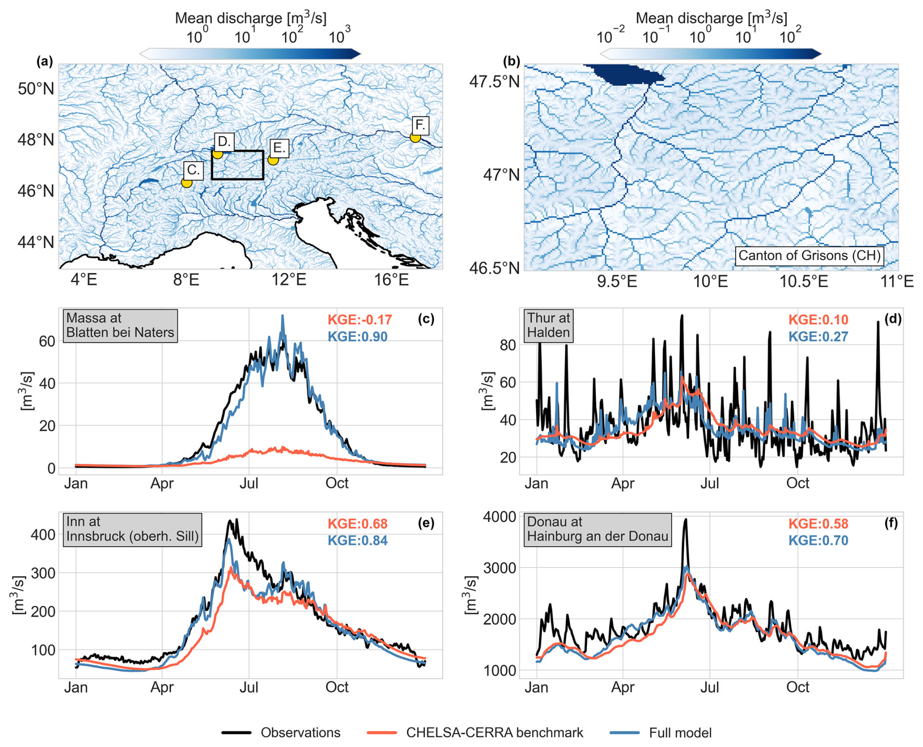
Figure 11 Illustration of the discharge simulations of the model with examples from hydrologically diverse river stations. (a) Average discharge (1990–2019) over the model domain. (b) Average discharge (1990–2019) over the Swiss canton of Grisons (inset shown in a in black). Panels (c)–(f) show climatologies (2010–2019) of observed vs. simulated discharge for the glacier-dominated Massa of Blatten (c), the rain-dominated Thur of Halden (d), the snow-dominated Inn of Innsbruck (e), and the larger river Danube of Hainburg (f).

In addition to discharge, LHMs also provide information on other variables such as SWE. Although there exist many local or national snow reanalysis products that are more accurate than our SWE simulations, semi-global products are often unrepresentative for mountain regions since their coarse resolution makes it difficult to represent complex terrain (Mortimer et al., 2020; Mudryk et al., 2025). Our analysis shows that our higher-resolution model setup outperforms coarser reanalysis products such as CERRA-Land and ERA5-Land, even without calibration (Fig. 5), but does not quite reach the performance of national-scale reanalysis products such as the OSHD product (Fig. 5g). Hyper-resolution LHMs could thus provide additional SWE products that bridge the quality gap between national and global datasets.

How suitable is the model for climate impact assessments, a typical application of hydrological models? While many larger-scale climate change impact assessments still use temperature-index-based approaches, including studies focusing on snow (e.g. Kraaijenbrink et al., 2021; Yang et al., 2022) or glaciers (e.g. Kraaijenbrink et al., 2017; Van Tiel et al., 2023; Hanus et al., 2024), there is discussion about the robustness of degree-day approaches under climatic change (Carletti et al., 2022). A short evaluation, which explicitly addressed model transferability, shows that model performance for discharge and SWE remains mostly consistent over the warmer and colder evaluation periods compared to the reference period, although the temperature changes over the study period are limited (Fig. S1 in the Supplement). Furthermore, we specifically aimed for increased robustness of parameters by focusing on SWE or glacier melt instead of streamflow during calibration. Sleziak et al. (2020) showed that the stability of hydrological model parameters such as DDFs across periods with different climate conditions can be increased by emphasizing snow representation during calibration. All of this suggests a reduced sensitivity of our model to increases in temperature. Still, the general caveats of the model remain applicable when extrapolating into the future. For example, the glacier module shows a realistic dynamic response to climate over larger regions but not necessarily for each individual glacier (Fig. 8). Users should be mindful of this uncertainty in individual glacier responses to climate change. Over time, continued glacier retreat will reduce glacier melt contributions to discharge since, globally, most glaciers have either already surpassed their peak in glacier melt contributions or will do so in the coming decades (Huss and Hock, 2018). This will lead rivers to shift towards more snow-dominated regimes (Farinotti et al., 2012). Further into the future (i.e. near the end of the century), the exact response of glaciers will thus be less important.

In summary, the presented model setup adds value to regional-scale hydrological studies, focusing on general patterns and on larger rivers which are nearly natural to moderately regulated. Caution should be used when interested in individual, small, or heavily regulated rivers, where catchment-scale models likely show better performance. Still, in regions with limited data availability, large-scale model runs with a global parameterization might remain the best option available, even for such small rivers.

5 Conclusions

Hydrological processes in mountain regions control the supply of water to dependent downstream regions and are therefore important well beyond the fringes of mountains. An accurate representation of these processes in LHMs is thus crucial, especially now that these models are moving towards higher spatial resolutions. In this paper, we proposed different model adjustments to the well-known and frequently used PCR-GLOBWB 2.0 model in its high-resolution version to make large-scale models better suited for applications in mountain regions. We studied how meteorological forcing and an improved representation of snow, glaciers, and soil affect discharge in the larger Alpine region. Based on our model evaluation, we conclude the following:

• Meteorological forcing is uncertain over alpine regions, and different forcing datasets lead to major differences in hydrological model performance for discharge. These performance differences vary spatially between different forcing datasets.

• Discharge simulations forced by a reanalysis product using high-resolution atmospheric dynamics at 5.5 km (CERRA-CHELSA) did not consistently outperform simulations with the other forcing products which use coarser atmospheric dynamics at 31 km (STANDARD and CHELSA; hypothesis 1 is not supported).

• An improved representation of snow and glaciers improves SWE and discharge simulations in high-alpine catchments where natural flow conditions dominate (hypothesis 2 is supported).

• The introduction of better runoff partitioning in the soil leads to an improvement of discharge simulations in smaller rain-dominated catchments by increasing their flashy response to rainfall peaks. However, these catchments still show overall weak model performance for discharge, suggesting that there is more to gain from improved routing in the soil (hypothesis 3 is supported).

• A major control limiting model performance for discharge in Alpine catchments is strong deviations from a closed water balance. Such deviations are sometimes related to hydropower plants or water transfers that are not accurately represented in the current model setup, which should be a priority in future model development.

• Finally, we present a new model setup with an improved representation of hydrological processes relevant in alpine regions which is well suited to studying regional and larger-scale streamflow and snow patterns in and around mountain regions. This new setup can be used to help quantify water resources and to study how these are impacted by human water use or climate in the Alpine region or around the world.

Appendix A: Sources for streamflow, catchment shapes, and reservoirs

(Klingler et al., 2021)Simmler (1961); Partl (1977)Speckhann et al. (2020, 2021)

Table A1 Agencies and databases as sources for data on streamflow, catchment shapes, and reservoirs.

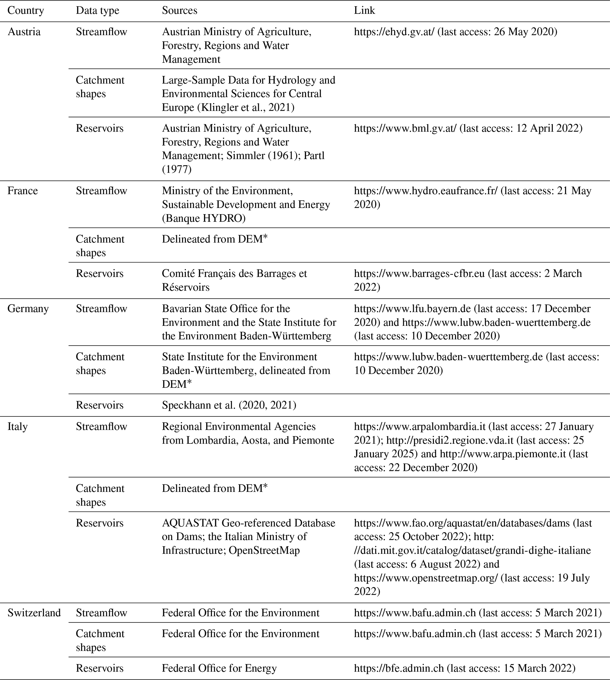
^* The DEM used is the COPERNICUS DEM (European Space Agency and Airbus, 2022).

Appendix B: Δh parameterization

The following detailed description of the Δh parameterization is based on Seibert et al. (2018a) and Huss et al. (2010).

Each glacier has a minimum surface elevation E_min and a maximum surface elevation E_max (both in metres above sea level). This topographic range of the glacier surface can be split into N elevation zones (in our case, into 20 steps, with E_min and E_max rounded to the nearest multiple of 50 m). Each elevation zone E_i with $\mathrm{1}<=i<=N$ is then normalized to

$$\begin{array}{}\text{(B1)}& E_{i,\text{norm}}={\displaystyle \frac{E_{\text{max}}-E_i}{E_{\text{max}}-E_{\text{min}}}}.\end{array}$$

The surface elevation of a glacier responds to glacier mass loss in a specific way that depends on its surface elevation. Huss et al. (2010) provided an empirical relationship between the normalized elevation zone E_i,norm and the normalized (unitless) change in the water equivalent of the glacier ice within this elevation zone Δh_i,norm:

$$\begin{array}{}\text{(B2)}& \mathrm{\Delta }{h}_{i,\text{norm}}=(E_{i,\text{norm}}+a{)}^{\mathit{\gamma }}+b(E_{i,\text{norm}}+a)+c,\end{array}$$

with a, b, c, and γ as empirical coefficients. Huss et al. (2010) provided three different sets of values for these empirical coefficients based on the initial surface area of the glacier.

Next, we need to couple this theoretical unitless ice thickness change to the actual observed mass loss. This is done by means of a scaling factor f_S. This scaling factor is the ratio between the total mass loss over the glacier ΔM (units of metres water equivalent) and the integrated normalized change in surface elevation, scaled by the surface area of the elevation zone A_i (as a fraction of the total glacier area).

$$\begin{array}{}\text{(B3)}& f_{\mathrm{S}}={\displaystyle \frac{\mathrm{\Delta }M}{{\sum }_{i=\mathrm{1}}^N{A}_i\cdot \mathrm{\Delta }{h}_{i,\text{norm}}}}\end{array}$$

Now, we can compute the new water equivalent for each elevation zone after a certain amount of mass loss:

$$\begin{array}{}\text{(B4)}& h_{i,k+\mathrm{1}}=h_{i,k}+f_{\mathrm{S}}\mathrm{\Delta }{h}_{i,\text{norm}},\end{array}$$

with k=0 as the initial glacier profile and h_i as the ice thickness (units of metres water equivalent) in each cell in that specific elevation zone. Huss et al. (2010) restricted surface elevation lowering at the edge of the glacier (where h<10 m). Here, we do not apply this because our grid cells are much coarser than those they used, and the ice thickness is thus almost never that thin. Finally, we make sure that cells cannot have less than 0 ice thickness. Any leftover mass loss is distributed over the rest of the glacier. Note that we apply this procedure to all glaciers independently of size. However, this scheme will hardly affect glaciers consisting of only a few cells, which are mostly governed by the mass balance per grid cell. For larger glaciers, this scheme becomes more important.