Exploring the ability of LSTM-based hydrological models to simulate streamflow time series for flood frequency analysis

An increasing number of studies have shown the prowess of long short-term memory (LSTM) networks for hydrological modelling and forecasting. One drawback of these methods is the requirement for large amounts of training data to properly reproduce streamflow events. For maximum annual streamflow, this can be problematic since they are by definition less common than middle or low flows, leading to under-representation in the model's training set. This study investigates six methods to improve the peak-streamflow simulation skill of LSTM models used for flood frequency analysis (FFA) in ungauged catchments. These include adding meteorological data variables, providing streamflow simulations from a distributed hydrological model, oversampling peak-streamflow events, adding multi-head attention mechanisms, adding data from a large set of “donor” catchments, and combining some of these elements in a single model. Furthermore, results are compared to those obtained by the distributed hydrological model HYDROTEL. The study is performed on 88 catchments in the province of Quebec using a leave-one-out cross-validation implementation, and an FFA is applied using observations, as well as model simulations. Results show that LSTM-based models are able to simulate peak streamflow as well as (for a simple LSTM model implementation) or better than (with hybrid LSTM–hydrological model implementations) the distributed hydrological model. Multiple pathways forward to further improve the LSTM-based model's ability to predict peak streamflow are provided and discussed.

1 Introduction

In the context of increasing global awareness regarding the impacts of climate change and urbanization, managing flood risks has become more critical than ever (Martel et al., 2021). Floodplain mapping and the design of hydraulic structures such as bridges, culverts, dams, and sewer systems play a vital role in mitigating flooding impacts (Apel et al., 2004). These tasks demand precise estimates of flood events with long return periods, such as the 20-year and the 100-year flood events.

The cornerstone of obtaining these critical design values lies in flood frequency analysis (FFA). FFA aims to estimate the likelihood of flood events of various magnitudes within a given time frame. This statistical analysis leverages long-term records of streamflow data, utilizing various models to predict the probability of extreme flood events (Laio et al., 2009). However, the reliability and accuracy of FFA are heavily contingent upon the availability of extensive streamflow time series (England et al., 2019). Long-term data are essential to reduce epistemic uncertainty and improve flood frequency estimations. Such comprehensive datasets enable a more accurate assessment of flood risks, which is critical in designing infrastructure capable of withstanding these natural disasters.

Yet, a significant challenge in conducting FFA is the scarcity of long-term hydrometric records. Many hydrometric gauges possess relatively short observational records. For example, a study by Do et al. (2017) showed that, from the Global Runoff Data Center database, only 3558 out of 9213 stations had more than 30 years of available streamflow data, with only 1907 stations having more than 38 years of data. This limitation can introduce substantial epistemic uncertainty into the FFA, potentially compromising the accuracy of flood risk assessments. For example, Hu et al. (2020) showed that the 100-year flood estimation had 50 % more uncertainty when using 35 years of data instead of the full 70-year record.

To overcome this limitation, methods have been developed to extend streamflow time series used to conduct FFAs. One such method is hydrological models to transform known meteorological data into streamflow. Traditionally, two types of hydrological models have been used for this task: lumped models and distributed models. These models can be trained over the study catchment (local or catchment models) or over a region (regional models) to extend the time series. Local models allow calibration of a model based on a single catchment and then extension of the period with meteorological data of the same catchment. Regional models, on the other hand, are designed to reproduce streamflow for a larger number of catchments within a region and are built specifically to be more robust over that sector. They can thus estimate streamflow at both gauged and ungauged locations within the region. Local models can also be used to simulate streamflow in ungauged locations, albeit with less accuracy, using regionalization methods (Arsenault et al., 2019; Arsenault and Brissette, 2014; Tarek et al., 2021).

The advent of deep learning has marked a significant shift in the approach to modelling hydrology. At the heart of this revolution are artificial neural networks (ANNs), a form of machine learning that mimics the way human brains operate (ASCE Task Committee on Application of Artificial Neural Networks in Hydrology, 2000). These networks consist of layers of interconnected nodes or “neurons”, with each layer being designed to recognize patterns of increasing complexity. Deep learning refers to the use of neural networks with many layers, enabling the modelling of highly complex patterns and relationships (LeCun et al., 2015). Among the various architectures of neural networks, recurrent neural networks (RNNs) and, more specifically, long short-term memory (LSTM; Hochreiter and Schmidhuber, 1997) networks, have shown particular promise in hydrological applications. Unlike standard feed-forward neural networks (ANNs), RNNs maintain memory across input sequences. This ability is crucial for processing time series data, where the relationship between sequential data points is vital for accurate predictions. LSTM networks further enhance this capability by incorporating mechanisms to remember and forget information over long sequences, making them ideally suited for modelling hydrological processes that depend on long-term dependencies (Kratzert et al., 2018; Shen and Lawson, 2021; Feng et al., 2020). Other machine learning algorithms have been tested in hydrology to estimate high flows. Convolutional neural networks (CNNs) combined with LSTM networks (CNN-LSTM; Li et al., 2022) improved high-flow simulations for a catchment in Germany. Hao and Bai (2023) showed that LSTM models performed better than support vector machines (SVMs) and extreme gradient boosting (XGBoost) for high flows, although XGBoost performed better for low flows. Research into deep learning methods in hydrology is ongoing, with novel methods such as temporal fusion transformers (TFTs) now showing promise for peak-flow simulation due to their integrated-attention mechanism (Rasiya Koya and Roy, 2024).

LSTM-based hydrological models have increasingly been utilized due to their ability to accurately simulate streamflow at both gauged and ungauged locations. These models can learn complex non-linear relationships between various hydrological variables and predict streamflow more accurately than conceptual or traditional hydrological models. They are thus prime candidates for extending streamflow time series. For instance, Kratzert et al. (2018) highlighted the superior performance of LSTM models over traditional models for simulating streamflow, while Shen and Lawson (2021) showed similar results at multiple river catchments, showcasing the model's ability to capture different hydrological conditions. Kratzert et al. (2019a) and Arsenault et al. (2023a) showed that LSTM models outperformed traditional hydrological models in streamflow regionalization by predicting streamflow at ungauged sites with more accuracy over a wide spatial domain. Wilbrand et al. (2023) advocated for using global datasets to improve streamflow prediction using LSTM networks after showing the strong potential over a large set of catchments worldwide. The strengths of LSTM-based modelling are now established in the literature, but some limitations still persist. A significant hurdle in the application of deep learning models to FFA is the need for extensive data to train them effectively. Given that extreme flood events are, by nature, rare occurrences, the scarcity of examples can limit the model's ability to learn and predict these events accurately. To address this challenge, researchers have explored various strategies, such as

1. incorporating additional variables such as climatic and land use data to better detect patterns (Wilbrand et al., 2023);

2. expanding the dataset to include more catchments, thus increasing the number of extreme-event examples (Fang et al., 2022);

3. artificial data augmentation by reintroducing copies of infrequent extreme events into the training datasets – this puts more weight on the optimization of model parameters by modifying the objective function's gradient (Snieder et al., 2021).

The main objective of this study is to determine whether LSTM-based hydrological models can generate accurate peak-streamflow predictions essential for effective flood risk management. By achieving this, more accurate and reliable FFA can be conducted in ungauged catchments.

2 Methods

2.1 Study area

The study area is composed of 88 catchments in southern Quebec, Canada. These catchments are important to the province for various reasons, including hydropower generation and agriculture. In the province of Quebec, floods are caused by three distinct processes. First, snowmelt is the main mechanism causing floods, especially over larger catchments (>1000 km²). This typically happens between the months of March and June, leading to one major flood event per year. Second are synoptic extreme rainfall events, which occur mostly in medium- to large-sized catchments (between 100 and 1000 km²), leading to similar or larger runoff volumes. These events can happen multiple times per year, but they can also not occur for multiple years. The third process is convective extreme rainfall events, which occur only in very small catchments or urbanized areas. The 88 selected catchments therefore mirror a representative set of Quebec rivers. Figure 1 presents the catchment locations, and Table 1 presents the main properties of these 88 catchments.

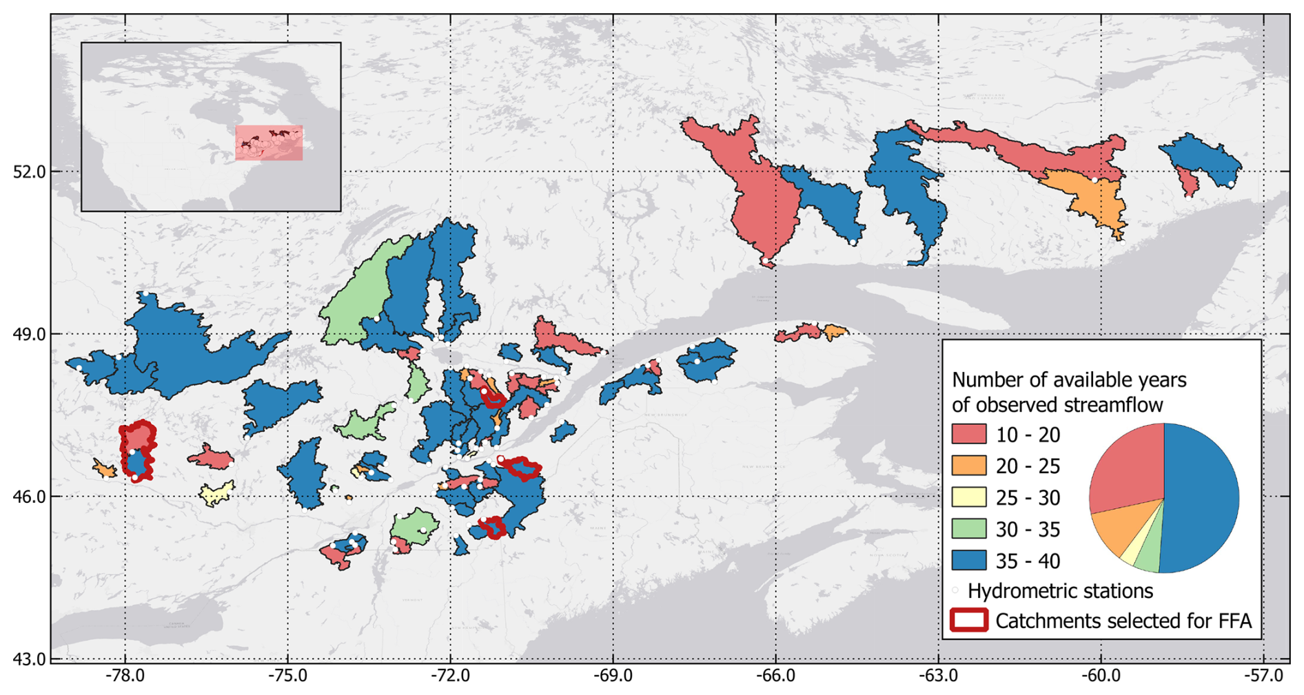
Figure 1 Study site of the 88 catchments in the province of Quebec. The colours represent the number of available years of observed streamflow for each catchment, and white circles represent the location of the catchment outlets. The four catchments with the red borders were selected for the FFA conducted in Sect. 3.2.

2.2 Data

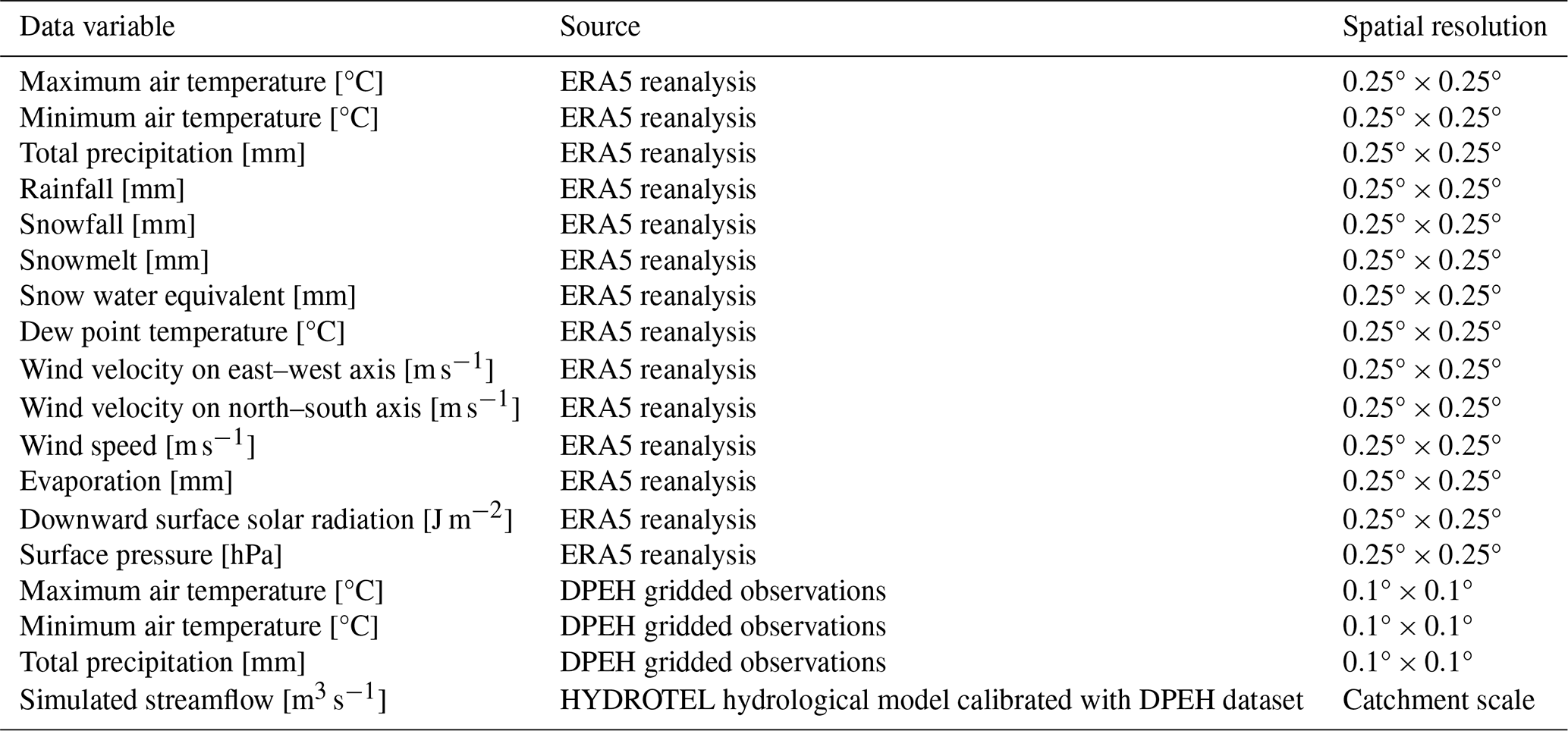
Multiple datasets were required for this project: meteorological data for model calibration and simulation, hydrometric data as the target of the modelling objectives, and catchment descriptors to provide regional information to the deep learning models to inform streamflow predictions.

2.2.1 Meteorological data

Two types of meteorological data were used in this study and are summarized in Table 1. First, we use an in-house gridded precipitation and air temperature dataset developed by the Quebec government using station observations (Bergeron, 2016). This product covers the period 1979–2017 and provides daily data at a 0.1° resolution. It was used to calibrate and perform simulations with the distributed hydrological model HYDROTEL. The HYDROTEL model was used as the benchmark against which to evaluate the LSTM networks, and its outputs were also used as an input into certain LSTM models, as described later.

The second type of meteorological data were from the ERA5 reanalysis product (Hersbach et al., 2020), which is provided by the European Centre for Medium-Range Weather Forecasts through their Climate Data Store (CDS). These data cover the entirety of the surface of the Earth at a resolution of 0.25° at an hourly timescale and were shown to be good proxies for observation stations for hydrological modelling (Tarek et al., 2020). Using ERA5 has the advantage of providing meteorological forcings without any missing data. This ensures a continuous spatial pattern for every day as opposed to the previous gridded dataset that must interpolate to fill in any missing data. ERA5 also provides more meteorological data than typical weather observation stations. Since LSTM models can ingest any number of variables as inputs, a set of hydrologically relevant variables were selected as potential predictors of streamflow. The list of variables is presented in Table 1. All variables were downloaded for the period 1979–2023 and processed to cover the same temporal domain as the observed streamflow at the 88 gauges of interest. Furthermore, the data were corrected for UTC offsets and aggregated at the daily time step to allow modelling at the same temporal resolution as HYDROTEL and the observed streamflow dataset. Finally, data were spatially averaged at the catchment scale to ensure that all catchments had the same number of input features for LSTM model training, enabling the use of regional LSTM model training, which has been repeatedly shown to be the best way forward for LSTM-based hydrological models (Arsenault et al., 2023a; Kratzert et al., 2024; Kratzert et al., 2019a, b).

Table 1 Summary of hydrometeorological variables used as inputs into the LSTM models in this study.

2.2.2 Hydrometric data

Hydrometric data were provided by the government of the province of Quebec, namely the water resources expertise directorate. These data are the official archives of the 88 stations containing daily average streamflow for each site. Depending on data availability, time ranges of station data cover the period 1979–2017. For this study, only stations with at least 10 years of available streamflow data were preserved to ensure sufficient data for training, validating, and testing the LSTM models, as well as providing a lower bound on the number of available years of extreme events for the FFA. Studies have shown that 15 years of data is the lower bound for LSTM-based modelling (Kratzert et al., 2018), but some strategies are implemented to mitigate this limitation. The catchments as depicted in Fig. 1 are colour-coded to indicate the number of available years of streamflow data for each station. The observed hydrometric data are also the target of the objective function for the LSTM and HYDROTEL model training and the basis against which the LSTM models are compared in this study.

2.2.3 Catchment descriptors

This study required a large set of catchment descriptors to help the LSTM models learn and build the relationships between meteorological time series and streamflow. To this end, 24 catchment descriptors were extracted using the PAVICS-Hydro platform (Arsenault et al., 2023b) for each catchment. A summary of these catchment descriptors is presented in Table S1 of the Supplement. Overall, there are eight descriptors related to the catchment shape and geographic properties (area, slope, elevation, aspect, Gravelius index, perimeter, centroid latitude, and centroid longitude), seven related to land use (fraction of crops, forests, grass, shrubs, water, wetlands, and urban), and nine related to hydrometeorology (mean snow water equivalent (SWE), mean potential evapotranspiration (PET), mean precipitation (pr), aridity index, fraction of precipitation falling as snow, frequency of high- and low-precipitation days, and duration of consecutive high- and low-precipitation days).

2.3 HYDROTEL

HYDROTEL is a semi-distributed physically based hydrological model with 27 parameters (Fortin et al., 2001b, a). HYDROTEL uses a modular approach to represent the main hydrological processes with various algorithms. Different sub-models can be selected to simulate snow accumulation and snowmelt, PET, channel routing, and the vertical water budget (Fortin et al., 2001b). For this study, the Hydro-Québec formulation (Fortin, 2000; Dallaire et al., 2021) was chosen to simulate PET, as well as a modified degree day estimating the daily evolution of the snowpack (Fortin et al., 2001a). The vertical water balance and channel routing are estimated with a three-layer soil model and a geomorphological hydrograph using the kinematic wave approximation.

The model requires both hydrometeorological and geomorphological information. Hydrometeorological data can be provided from observation sites or gridded datasets at daily and sub-daily time steps. The modules selected for this study require daily series of total precipitation, as well as minimum and maximum temperatures. The geomorphological information of each catchment is first processed by PHYSITEL (Rousseau et al., 2011), a GIS-based software that prepares catchment information (e.g., topography, soil type, land use). PHYSITEL divides the catchment into relatively homogenous hydrological units (RHHUs), whereas HYDROTEL estimates hydrological processes.

This hydrological model has been used in the study region for diverse applications, including extreme flood simulations (Lucas-Picher et al., 2015), climate change impact studies (Castaneda-Gonzalez et al., 2023), and regionalization methods (Martel et al., 2023), and is currently applied in an operational context by the DPEH for climate change impact studies and daily hydrological forecasting in the province of Quebec (CEHQ, 2015).

A regional HYDROTEL model, pre-calibrated by the DPEH, served as the baseline for local recalibration on each of the selected 88 catchments. These locally calibrated models were then used in this study for comparison purposes and as an input for the LSTM-based hydrological model structures.

2.3.1 Regional model

The HYDROTEL platform used in this study was set up by the DPEH. The platform consists of 15 large regions covering 771 403 km² in southern Quebec and (to a lesser extent) the province of Ontario and the United States (CEHQ, 2015). The DPEH provided a fully calibrated HYDROTEL platform that includes 259 calibrated gauges. This pre-calibrated HYDROTEL platform consists of two globally calibrated regions. In other words, one set of parameters was obtained for the gauges located on the northern shore of the St Lawrence River, and another one was obtained for the regions located on the southern shore.

2.3.2 Local recalibration

A local recalibration was performed on each of the 88 selected catchments to ensure their best local performance. From the 27 internal parameters of HYDROTEL, 11 parameters were recalibrated, and the remaining 16 were fixed following the previous recommendations of Turcotte et al. (2007) (see Table S2 of the Supplement). This recalibration was performed using the Dynamically Dimensioned Search (DDS) algorithm (Huot et al., 2019; Tolson and Shoemaker, 2007) and the Kling–Gupta efficiency criterion (KGE; Gupta et al., 2009; Kling et al., 2012) as objective functions over the entire period of 1979–2017. The idea behind using the entire period is that the models may benefit from longer periods of data, especially with the limited number of peak-streamflow events. This has been proposed in recent studies that highlighted the importance of including all available data in a final calibration to ensure a more robust set of parameters (Arsenault et al., 2018; Mai, 2023; Shen et al., 2022).

2.4 LSTM-based hydrological model structures

The different elements of the model structures are described in the following subsections.

2.4.1 General LSTM structure

In this study, a series of deep learning models that leverage LSTM networks were implemented to model hydrological processes within catchments. The model architecture is designed to process both dynamic and static inputs, reflecting the temporal dynamics and invariant characteristics of the catchments, respectively.

The dynamic component of the model ingests time series data, specifically designed to handle 365 d input sequences preceding the target day. Once constructed, this input is processed through six parallel LSTM branches, each consisting of two initial LSTM layers with 128 units, followed by concatenation and another LSTM layer to further refine the temporal features. This design choice aims to capture a broad range of temporal dependencies and patterns within the data. Each branch incorporates a dropout layer with a rate of 0.2 to prevent overfitting. The outputs of all branches are then concatenated and processed through a final LSTM layer to synthesize the temporal information into a cohesive representation.

In parallel, the static inputs are processed through a dense layer with 256 units with a rectified linear unit (ReLU) activation function to introduce non-linearity. A dropout rate of 20 % is again applied. The processed dynamic and static features are then concatenated to form a comprehensive representation of the hydrological state. This combined feature vector is then passed through a dense layer of 256 units including a “Leaky-ReLU” activation function. Finally, the outputs of this layer are passed to a single, ReLU-activated dense layer with a single unit. The final output is the prediction of the target variable, i.e., the streamflow value.

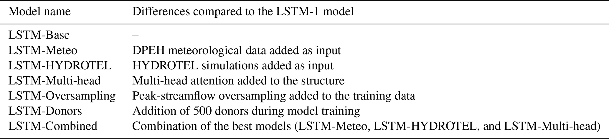
This general deep learning model was implemented in multiple variants by adjusting certain inputs, structures, and hyperparameters to evaluate their ability to improve peak-flow simulation. The first variant, considered to be the reference LSTM model (referred to as “LSTM-Base” in this study), used the structure described here and presented in Fig. S1. It was driven using all catchment descriptors but only the ERA5 meteorological data as dynamic features.

2.4.2 Addition of dynamic datasets

The first test to improve upon the LSTM-Base model was to increase the number of input variables by adding the daily precipitation and minimum and maximum air temperature from the DPEH dataset. While LSTM-Base already includes the same variables from the ERA5 dataset, it was previously shown that adding the same variables originating from different datasets (such as observations, gridded or interpolated datasets, or reanalysis data) could help improve hydrological model simulations in a multi-model, multi-input setting (Arsenault et al., 2017). For example, Kratzert et al. (2021) show that providing three different meteorological datasets to an LSTM model improved performance compared to using the LSTM models trained on each individual dataset. In this study, the model that integrates a supplementary dataset is referred to as “LSTM-Meteo”, and it uses the same structure and hyperparameters as LSTM-Base.

Another similar test was performed in which the simulations generated by the calibrated HYDROTEL hydrological model were added to the LSTM-Base model as a dynamic input. These hydrographs can be used as inputs to introduce “expert” knowledge into the model. Indeed, this can be used by the LSTM model as a starting point to converge toward a reasonable solution, using the ERA5 time series data to determine corrections or to detect other patterns to further improve upon the HYDROTEL simulations. This process has been performed before for general hydrological modelling and has shown better performance than process-based models or LSTM models individually (e.g., Liu et al., 2022; Wei et al., 2024; Nearing et al., 2020). The resulting model is referred to as “LSTM-HYDROTEL” in this study.

2.4.3 Multi-head attention

Multi-head attention mechanisms, when integrated with LSTM models, enhance the model's ability to process and interpret sequential data by allowing the model to focus on different parts of the input sequence simultaneously (Vaswani et al., 2017). LSTM networks are inherently designed to remember information for long periods, and the addition of multi-head attention enhances this capability by providing a more nuanced understanding of the sequence. This is particularly beneficial in tasks that involve complex dependencies over long sequences, which are common in hydrological modelling (Wang et al., 2023). Examples include snow accumulation and snowmelt and baseflow contributions to streamflow depending on precipitation and evapotranspiration in the previous weeks and months.

The essence of a multi-head attention mechanism is its capability to generate multiple attention “heads”. Each head learns to attend to different parts of the input sequence, capturing various aspects of the sequence's contextual relationships. This is achieved by parallelizing the attention process, enabling the model to aggregate information from different representational subspaces at different positions within the sequence. In this study, four heads of 32 nodes each were implemented in the model, referred to as the LSTM-Multi-head. This mechanism was implemented in four of the six parallel branches of the LSTM-Base model, such that two parallel branches remain without the attention mechanism, to preserve some direct link to the previous models of LSTM-Base, LSTM-Meteo, and LSTM-HYDROTEL. The structure of the multi-head attention model can be found in Fig. S2.

2.4.4 Oversampling

In addressing the challenge of accurately modelling peak-streamflow events, a data augmentation strategy, namely oversampling, was implemented. The rationale is to ensure that more extreme values are used during the optimization process, forcing the weights of the model to account for these events more heavily during training (Snieder et al., 2021). This artificial enhancement of the representation of peak-streamflow events addresses the inherent imbalance in the dataset, where such events are vastly outnumbered by more common, lower-magnitude streamflow conditions.

The initial step was the identification of peak-streamflow events within the observed streamflow data. Peak-streamflow events are defined as those observations that fall within the top 1 % of all streamflow values recorded in the dataset. This criterion ensures that only the most extreme streamflow conditions are selected for augmentation, focusing the model's learning capacity on these critical events. Then, each selected peak-streamflow event is replicated and reinjected into the training dataset. Specifically, each event is copied and randomly inserted into the training data 10 times. This approach significantly increases the presence of peak-streamflow events in the training set, thereby providing the model with more examples of these extreme conditions to learn from during mini-batch gradient descent and weight optimization.

This version of the LSTM model, referred to as “LSTM-Oversampling”, uses only the ERA5 meteorological data as dynamic features, along with the full set of static features. It also uses the same structure and hyperparameters as the models LSTM-Base, LSTM-Meteo, and LSTM-HYDROTEL.

2.4.5 Additional donors

To enhance the robustness and generalizability of our LSTM model, the training dataset was expanded beyond the initial 88 catchments by incorporating data from an additional 500 catchments. These catchments were taken from the HYSETS database, a dataset containing hydrometeorological data and catchment descriptors for over 14 000 catchments in North America (Arsenault et al., 2020a; 2020b). Catchments were selected from the HYSETS database according to the following criteria:

• located near the region of interest, bounded by a latitude of [37°; 59°] and a longitude of [−51°; −90°];

• shows a drainage area between 50 and 50 000 km²;

• has a minimum of 20 years of observed streamflow data available.

From these catchments, 500 were randomly selected, providing a wider range of data for the LSTM model. The added variability from the supplementary donors should thus provide more diverse training data, allowing the LSTM models to better learn the relationships between meteorological and hydrometric time series, as shown in Fang et al. (2022). This “LSTM-Donors” model uses the same setup as LSTM-Base but with data from 588 catchments instead of 88.

2.4.6 Combined model

The final LSTM model variant combines the structure of the LSTM-Multi-head model with the extra meteorological data from LSTM-Meteo and the HYDROTEL-simulated streamflow from LSTM-HYDROTEL. Oversampling was tested but was shown to worsen results, leading to it being discarded from this combined model. Furthermore, it was also not possible to add the 500 extra donors into this model as HYDROTEL had not been implemented at those catchments. This combined model is referred to as the “LSTM-Combined” model in this study. Table 2 presents a summary of the seven LSTM model variants for convenience.

Table 2 Variants of the LSTM-based hydrological models used in this study.

2.5 LSTM model training

The seven variants of the LSTM models were developed to minimize the standardized Nash–Sutcliffe efficiency (NSE; Nash and Sutcliffe, 1970) loss function. This objective function was chosen due to its effectiveness in quantifying the predictive accuracy of hydrological models, where a higher NSE value indicates better model performance. However, given that multiple catchments are processed at the same time, streamflow was standardized by the size of the catchment to prevent larger catchments with higher streamflow from dominating the NSE. This method was first implemented for LSTM models and was successfully applied in a previous streamflow regionalization study using LSTM models (Arsenault et al., 2023a).

Prior to training, all variables were normalized using a standard scaler. This step is crucial for ensuring that the LSTM models could efficiently learn from the data as it mitigates the issue of different scales among the input features, which can significantly affect the convergence speed and stability of the training process. The models were then trained using the “AdamW” optimizer, an extension of the Adam optimization algorithm that includes weight decay to prevent overfitting (Loshchilov and Hutter, 2017, 2018). The training process was conducted over 300 epochs, with an early stopping mechanism. Specifically, the training would halt if there was no improvement in the validation loss for a patience period of 25 epochs. This approach ensures that the model does not overfit to the training data and can generalize well to unseen data. To further enhance the training process, a “reduce learning rate on plateau” strategy was employed. This technique dynamically adjusts the learning rate when the validation loss stops improving for better convergence. In this study, the plateau duration was set to 8 epochs with a factor of 0.5, reducing the learning rate by 50 % three times before the 25-epoch patience is attained.

All LSTM models were trained regionally, using the datasets from the 88 catchments, providing a comprehensive and diverse range of hydrological behaviours for the LSTM models to learn from. The temporal data from each catchment were divided into three subsets: training, validation, and testing. The first 60 % of the available data for each catchment were used for training, the subsequent 20 % were used for validation, and the final 20 % were used for testing. This division ensures that the models are trained on a substantial portion of the data while still being validated and tested on distinct sets to evaluate their generalization performance accurately.

2.6 Evaluation of peak-streamflow representation

To assess the performance of the LSTM models in hydrological modelling of catchments and, in particular, peak streamflow, two metrics were employed. These are the Kling–Gupta efficiency (KGE) and the normalized root mean square error (NRMSE) of the Qx1day index. Both metrics were evaluated based on the 88 individual catchments after model training, comparing the LSTM-simulated streamflow to the observed streamflow. As a reference, results obtained using the HYDROTEL model (which was used in the calibration) are also evaluated using these same metrics.

The Kling–Gupta efficiency (KGE; Gupta et al., 2009; Kling et al., 2012) is a widely used metric in hydrology that evaluates the overall performance of hydrological models by comparing simulated and observed values in terms of correlation, bias, and variability. It is defined as

$$\begin{array}{}\text{(1)}& \mathrm{KGE}=\mathrm{1}-\sqrt{{\left(r-\mathrm{1}\right)}^{\mathrm{2}}+{\left(\mathit{\alpha }-\mathrm{1}\right)}^{\mathrm{2}}+{\left(\mathit{\beta }-\mathrm{1}\right)}^{\mathrm{2}}},\end{array}$$

where r is the Pearson correlation coefficient between observed and simulated streamflow, α is the ratio of the standard deviation of simulated streamflow to that of observed streamflow, and β is the ratio of the mean of simulated streamflow to that of observed streamflow. A KGE value of 1 indicates perfect agreement between simulated and observed data, while a value that is closer to 0 or negative indicates poor model performance.

For evaluating the model's accuracy in predicting extreme streamflow events, we utilize the normalized root mean square error (NRMSE), specifically applied to the Qx1day metric. The Qx1day metric represents the maximum simulated and observed 1 d streamflow event for each year, focusing on the model's ability to capture extreme hydrological phenomena. The NRMSE for Qx1day is calculated as follows:

$$\begin{array}{}\text{(2)}& \mathrm{NRMSE}\mathrm{of}\mathrm{Qx}\mathrm{1}\mathrm{day}={\displaystyle \frac{\sqrt{\frac{\mathrm{1}}{n}{\sum }_{i=\mathrm{1}}^n{\left(Q_{\mathrm{obs},i}^{\mathrm{1}\mathrm{d}}-Q_{\mathrm{sim},i}^{\mathrm{1}\mathrm{d}}\right)}^{\mathrm{2}}}}{{\mathit{\sigma }}_{Q_{\mathrm{obs}}^{\mathrm{1}\mathrm{d}}}}}.\end{array}$$

Here, $Q_{\mathrm{obs},i}^{\mathrm{1}\mathrm{d}}$ and $Q_{\mathrm{sim},i}^{\mathrm{1}\mathrm{d}}$ denote the observed and simulated maximum 1 d streamflow events, respectively; n is the total number of such events considered; and ${\mathit{\sigma }}_{Q_{\mathrm{obs}}^{\mathrm{1}\mathrm{d}}}$ is the standard deviation of the observed 1 d streamflow events. This metric specifically addresses the model's precision in forecasting the magnitude of peak-streamflow events, with lower values indicating higher accuracy.

2.7 Flood frequency analyses

To assess the suitability of the annual maximum series (AMS) for flood frequency analysis (FFA), analyses were carried out on a selection of catchments using extreme-value theory to estimate peak-flow quantiles associated with various return periods. The GEV (generalized extreme value) distribution, derived from the block maxima method, was used as it is specifically designed to model the behaviour of annual extremes (Coles et al., 2001). Within the GEV family, the Gumbel distribution – also known as the extreme-value type-I distribution (EV-I) – represents a special case where the shape parameter is fixed at zero, reducing the distribution from a three-parameter form to a two-parameter form.

Although the GEV distribution generally offers greater flexibility and a better fit to extreme-value data, the estimation of its shape parameter can be unreliable when the AMS record is short. This limitation is common in streamflow time series. To address this, both the GEV and Gumbel distribution parameters were estimated using the maximum likelihood method (MLM), and their performance was compared using the likelihood ratio test (LRT). The LRT, appropriate for nested models such as the GEV and Gumbel, assesses whether the inclusion of the shape parameter in the GEV leads to a statistically significant improvement in model fit.

To construct empirical frequency plots, the Cunnane plotting position was applied to estimate the non-exceedance probability associated with each annual maximum value (Cunnane, 1978). The Cunnane formula is given by

$$\begin{array}{}\text{(3)}& P={\displaystyle \frac{m-\mathrm{0.4}}{n+\mathrm{0.2}}},\end{array}$$

where P is the non-exceedance probability, m is the rank (with m=1 being the smallest value), and n is the total number of observations. This method provides an approximately unbiased estimate of extreme quantiles and is widely used in hydrological frequency analyses, including those conducted by Environment and Climate Change Canada (ECCC). While the Gringorten plotting position is theoretically better suited for the Gumbel distribution (In-na and Nyuyen, 1989), the Cunnane formula was adopted uniformly in this study to ensure methodological consistency across all cases, especially given that model selection was based on statistical testing rather than a priori preference.

3 Results

3.1 Training, validation, and testing period results

The first results presented are those related to the model training, validation, and testing of the LSTM models. The results of the HYDROTEL model are also presented as a reference. Figure 2 presents the KGE and NRMSE Qx1day (which will be shortened to “NRMSE” in the text for clarity) results for each of the three periods. The periods vary from catchment to catchment, and the training, validation, and testing phases represent 60 %, 20 %, and 20 % of the overall available data for each catchment, respectively.

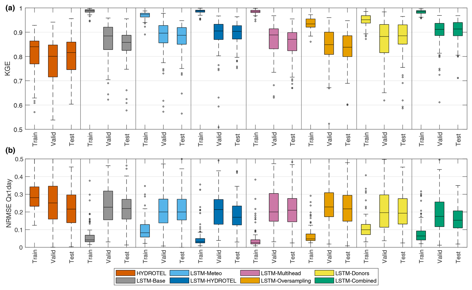
Figure 2 KGE and NRMSE of Qx1day for the 88 catchments when modelled with the HYDROTEL hydrological model and seven LSTM model variants. Results are presented according to the training, validation, and testing periods.

From Fig. 2, it can be seen that the HYDROTEL model performance is relatively stable for both metrics across all three periods. This reflects the fact that HYDROTEL was calibrated based on the entire period. On the other hand, LSTM models are completely blind to the testing period data. The LSTM models all display better KGE results than HYDROTEL, showing the strong capacity of regional LSTM models to simulate streamflow for individual catchments and also confirming that the LSTM-based models were not subject to overfitting. Results also differ significantly within the LSTM model variants. First, simply adding the three meteorological variables (maximum and minimum temperature and precipitation, which were already represented in the ERA5 data) improves results, as was the case in Arsenault et al. (2017) for multi-model averaging implementations. Then, it can be seen that simply adding the HYDROTEL model simulations as inputs dramatically increases the KGE, meaning that the LSTM is able to use the simulated streamflow as inputs but can correct them similarly to a post-processing implementation. The multi-head implementation had mixed results depending on the catchment, but the oversampling strategy led to worse results than the LSTM-Base model. The LSTM-Donors model led to very promising results similar to those of LSTM-Meteo. Finally, the LSTM-Combined model showed the best performance, indicating that adding more information and giving the model more flexibility within its structure is an advantageous strategy. Results for NRMSE show similar trends but with less dominance over HYDROTEL. This could be related to the limited number of peak-streamflow events for training the LSTM models, which is one of their shortcomings. Nonetheless, the LSTM-Meteo, LSTM-HYDROTEL, and LSTM-Combined models provide notably better NRMSE results than the calibrated HYDROTEL model.

To further evaluate the relative performance of each model, results were compared on a per-catchment basis. Figure 3 presents a summary of the testing period results for KGE and NRMSE (Fig. 3a and b, respectively), as well as a map of the best-performing models for each metric (Fig. 3c and d) and, finally, a comparison between the HYDROTEL model and the LSTM-Combined model (Fig. 3e and f), which displays the best performance.

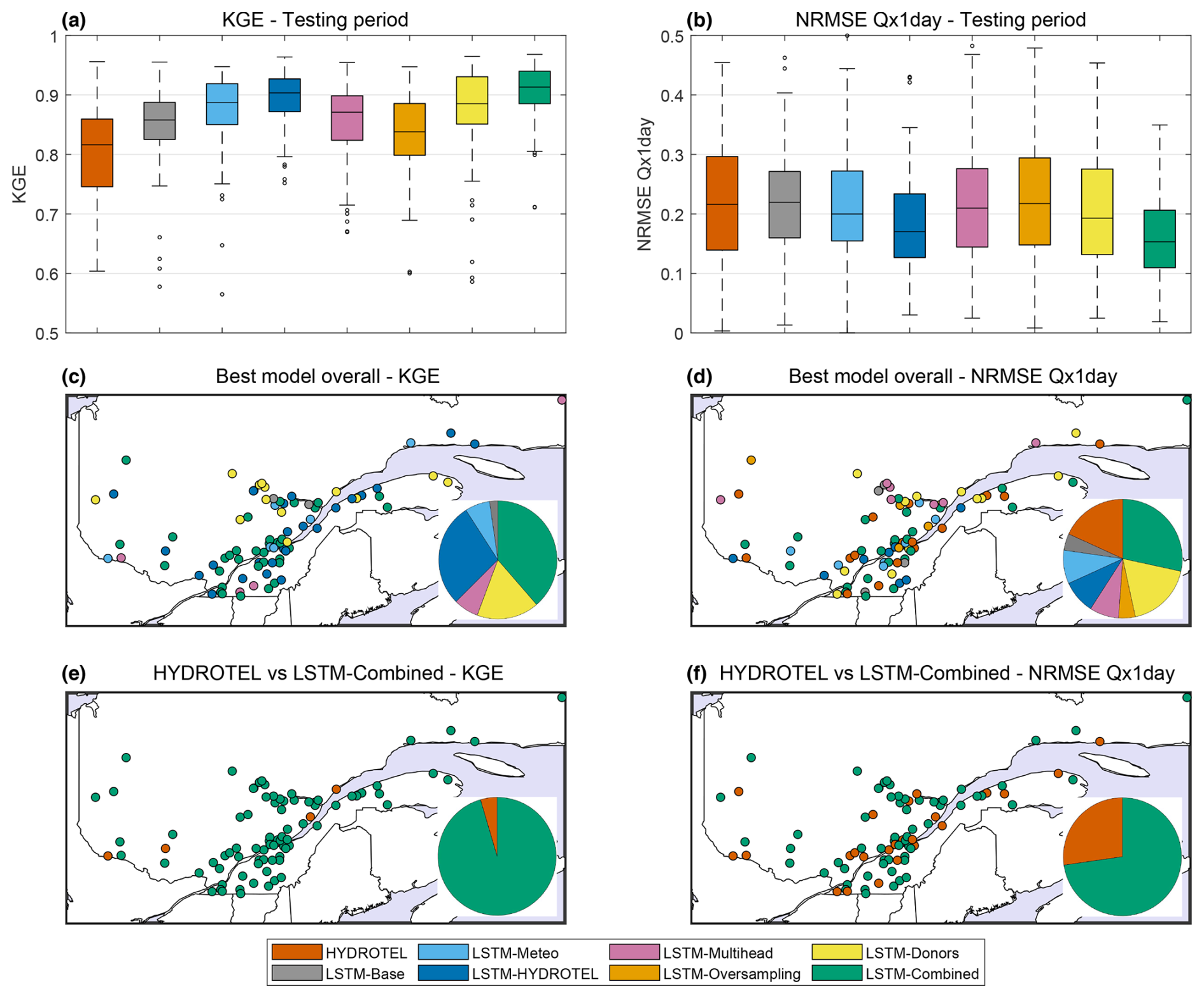
Figure 3 Results over the testing period for the 88 catchments for the KGE (a, c, e) and NRMSE of Qx1day (b, d, f). Rows present the overall performance for the eight models (HYDROTEL and seven LSTM variants; a, b), maps representing the best-performing model for each of the 88 catchments (c, d), and maps presenting the best model – between HYDROTEL and LSTM-Combined – for each catchment (e, f). The pie charts represent the distribution of the best model.

Figure 3 shows that the LSTM-Combined model is the best-performing model according to the KGE metric, owing to its strong general streamflow simulation skill. For the NRMSE, the picture is more nuanced, with the eight models sharing the top rank for the 88 catchments, with no clear spatial pattern that would allow for the prediction of a “best model” based on catchment location. The LSTM-Combined model was selected in 38.6 % (Fig. 3c) and 28.4 % (Fig. 3d) of the catchments for the KGE and NRMSE, respectively, compared to 0 % and 18.2 % for HYDROTEL. When only the HYDROTEL and LSTM-Combined model are compared, the latter shows better performance in terms of KGE evaluation (95.5 %; Fig. 3e) and outperforms HYDROTEL in a majority of catchments for the NRMSE (72.7 %; Fig. 3f), although the results are, again, more nuanced.

Figure 4 (NRMSE Qx1day) and Fig. S3 (KGE) present the results of a supplementary analysis done to evaluate the performance of the models as a function of catchment size to determine if it could help predict model skill. Similarly, Fig. S4 (NRMSE Qx1day) and Fig. S5 (KGE) present the comparison between the performance of models as a function of the number of available years. Note that only Fig. 4 is shown in the text; Figs. S3, S4, and S5 are presented in the Supplement.

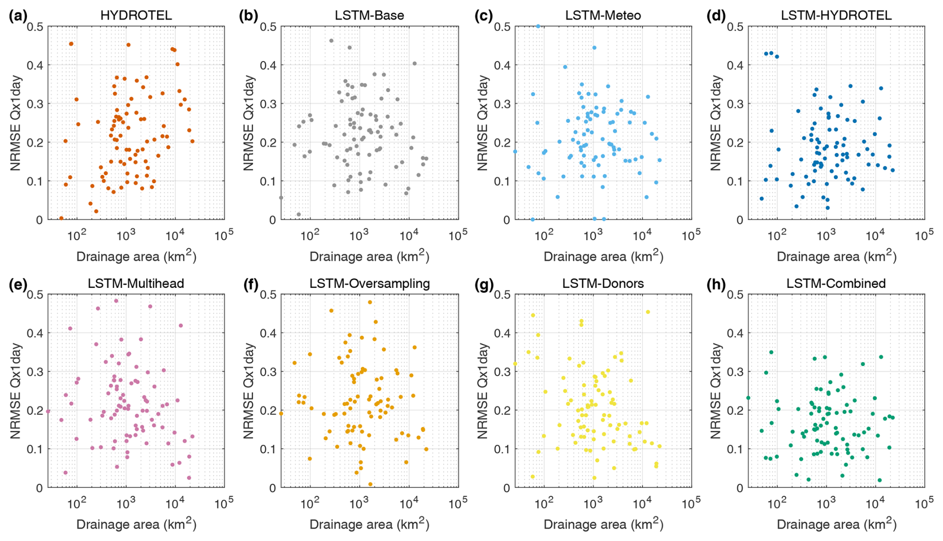
Figure 4 NRMSE of Qx1day scores for each of the eight models based on the 88 catchments as a function of the catchment drainage area.

As can be seen in Figs. 4 and S3, the drainage area of the catchments on a logarithmic scale does not seem to impact the LSTM model variants. Indeed, the scatterplots obtained suggest that no correlation would be found from fitting a linear regression. Only two models were found to be statistically significant with relatively small Pearson's linear correlation coefficients: LSTM-Multi-head (KGE = 0.31 and NRMSE = −0.28) and LSTM-Donors (KGE = 0.30 and NRMSE = −0.25).

The analysis revealed no significant correlations between the number of available years and the model performance (both KGE and NRMSE Qx1day) for either hydrological model. This suggests that model performance is not directly influenced by the length of the observational record.

3.2 Detailed evaluation on four selected catchments

The next results show the peak streamflow for each year in the datasets of four selected catchments with almost full observational records (catchment nos. 061022 and 023303 are missing 1984 and 1980, respectively), including for the training, validation, and testing periods. These catchments were selected to represent a relatively small catchment and a large catchment in both northern (3756 and 490 km²) and southern (1152 and 769 km²) regions (see Fig. 1). They are also the same as those that are analyzed in detail in Martel et al. (2023). Results of this analysis are presented in Fig. 5.

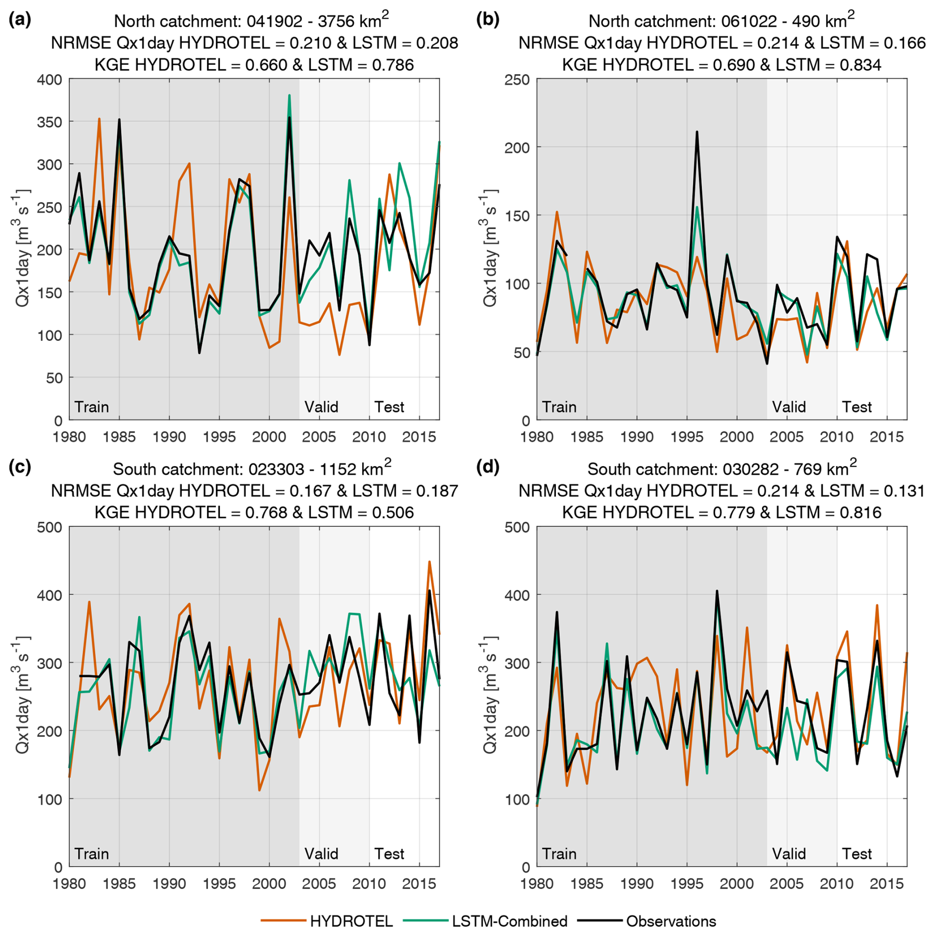
Figure 5 Qx1day of each year in the training, validation, and testing periods for four representative catchments for HYDROTEL, LSTM-Combined, and the observed streamflow. The four catchments represent a large northern (a), small northern (b), large southern (c), and small southern (d) catchment. The NRMSE values of the Qx1day for HYDROTEL and the LSTM-Combined model during the testing period are shown in each figure's title.

Results in Fig. 5 show multiple interesting elements that can help understand the strengths and limitations of the HYDROTEL and LSTM-Combined models. First, the training period clearly demonstrates that the LSTM-Combined model is able to fit the data with surprising accuracy on most occasions, except for some extreme events in the observations (either low or high, such as for the years 1980 and 1998 in catchment no. 061022, Fig. 5b). The validation period, which serves as the stopping criteria evaluation for the LSTM training process, is not directly used in training but is still used to determine the best parameter set, meaning that it is not independent. This can be seen in Fig. 6 where the LSTM-Combined validation period Qx1day values are more similar to the observations compared to the HYDROTEL simulations. However, the more interesting case is for the testing period. Overall, the LSTM-Combined model outperforms HYDROTEL again; however, HYDROTEL performs best for the large catchment in southern Quebec (Fig. 5c). It can also be seen that, overall, the performance during the testing period is worse than during the training and validation periods for the LSTM-Combined model. However, HYDROTEL shows similar errors across all periods, again due to the fact that it was calibrated based on the entire period and therefore preserved similar skill during all three periods.

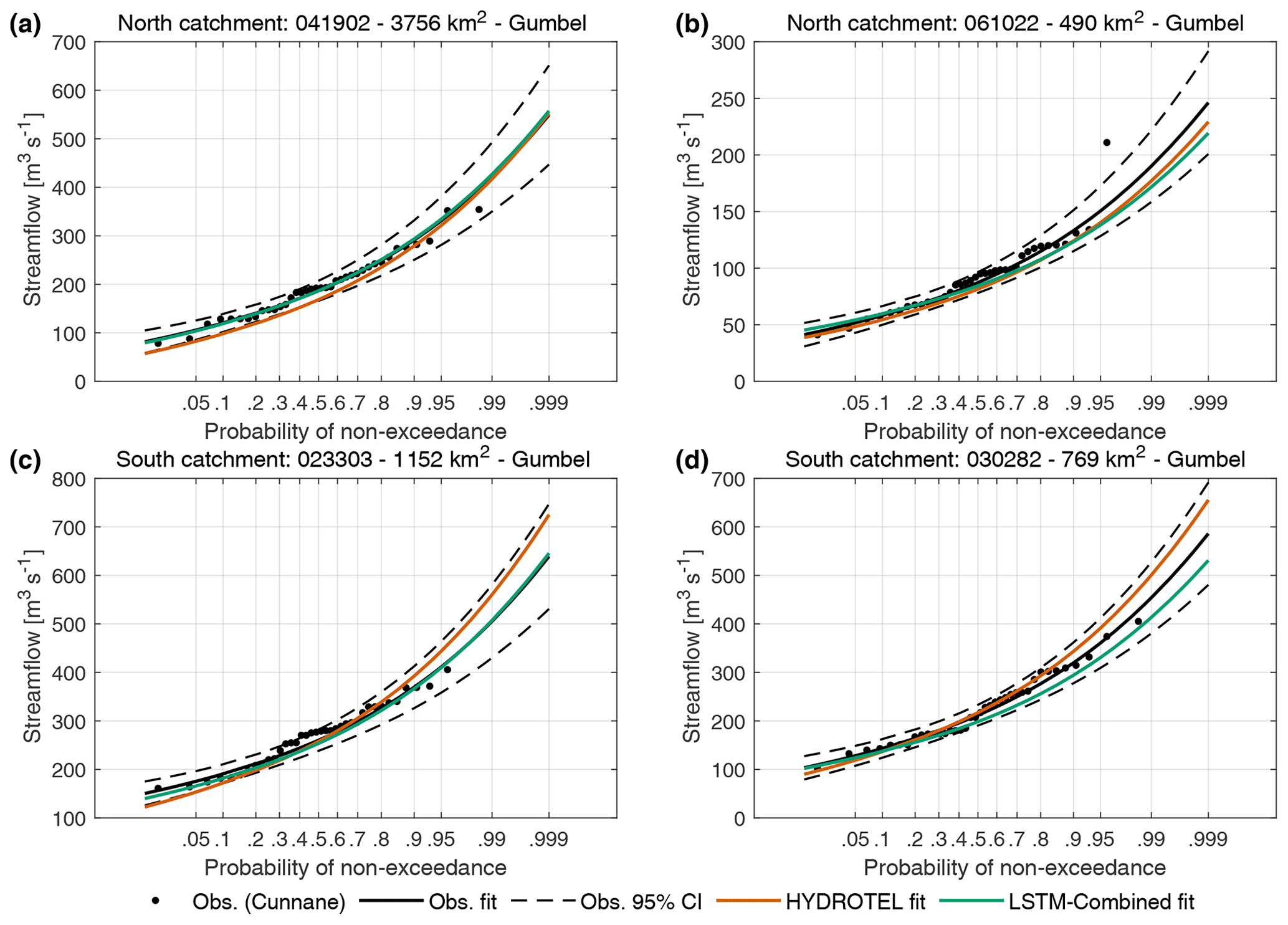
Figure 6 Flood frequency analysis for the four selected catchments: northern–large (a), northern–small (b), southern–large (c), and southern–small (d). Results are shown for the HYDROTEL model and for the LSTM-combined model.

Finally, results for the FFA are presented in Fig. 6 for the four selected catchments. Results of the LRT indicated that the Gumbel distribution provided an adequate and more parsimonious fit for all four catchments examined (see Fig. 6), with no significant gain from using the full GEV formulation. Consequently, the Gumbel distribution was selected as the preferred model for FFA and was fit to the observations, as well as to the HYDROTEL and LSTM-combined model AMS.

It can be seen in Fig. 6 that the LSTM-Combined and HYDROTEL model FFAs fall within the uncertainty bounds of the observations. However, it is interesting to note that the LSTM model seems to either match or underestimate the observed distribution, while HYDROTEL shows both overestimation and underestimation.

4 Discussion

4.1 Strengths and weaknesses of each model in streamflow simulation

In this paper, LSTM-based deep learning models are compared to a distributed hydrological model for peak-streamflow simulation. The HYDROTEL hydrological model was calibrated over the entire period, whereas the LSTM-based models were trained and evaluated based on distinct periods, leading to a less favourable outcome for the LSTM models. Nonetheless, when the results are compared for the LSTM validation period, it can be seen that the LSTM models outperform the HYDROTEL model in most cases for overall streamflow simulation (KGE metric) and are at least as good in terms of peak streamflow (NRMSE Qx1day metric) depending on the LSTM modelling strategy, as displayed in Figs. 2 and 3.

As for the peak streamflow specifically, the two best models are those that include HYDROTEL simulations. This is a clear signal that the LSTM models are able to learn from the first estimation of hydrological models and improve them further using exogenous data. The other LSTM models tested provided mixed results depending on the catchments (Fig. 3b, d, and f) even though they outperformed HYDROTEL in terms of the KGE metric. This clearly displays the limitations of LSTM models regarding peak streamflow. Indeed, while the attention mechanism, the oversampling, and the addition of other meteorological data improved the overall simulation performance, the inherent lack of rare events in the training dataset limits the LSTM model's ability to generate these important streamflows.

The addition of meteorological data to the LSTM-base improved results, indicating that there is additional information that is not present in the original dataset and that LSTM models can extract this added information. For example, it is possible that the datasets reflect slight differences in meteorological statistics based on their generation method, which could lead to biases. The LSTM could use these as a multi-input method to correct biases, as in Arsenault et al. (2017). These results mirror those of Kratzert et al. (2021).

The multi-head attention LSTM was unable to improve results in an appreciable manner compared to the LSTM-Base model. This could lead to overfitting and could be evaluated in another study with smaller model structures. For this case, results suggest that the LSTM-Base model had sufficient complexity to maximize the performance from the available data, limiting the potential of the multi-head implementation. The attention mechanism, similarly, did not provide the desired increase in weights based on the peak streamflow, again, probably due to the few cases in the training period.

The LSTM-Oversampling model was the worst-performing model in this study in terms of peak streamflow, with worse results than the HYDROTEL model. However, this failed, still providing better KGE values than HYDROTEL but worsening the NRMSE Qx1day estimation. This implementation was rather rudimentary, and recent research has shown that some oversampling or undersampling methods could perform better, including generating synthetic data from regressions between under-represented datasets (i.e., Synthetic Minority Over-sampling Technique; Maldonado et al., 2019; Wu et al., 2020).

Finally, the LSTM-Donors model provided interesting results given the fact that it used the same data types as the LSTM-Base model and performed better in terms of both the KGE and NRMSE Qx1day metrics. Using more catchments ensures that more peak-streamflow events are seen during training.

4.2 On the effect of adding hydrological model simulations to the inputs of an LSTM network

The addition of the HYDROTEL simulations to the LSTM network was done to guide the LSTM network in terms of physics that the LSTM network alone cannot implement. For example, deep learning networks lack the ability to ensure that mass balance is respected and have no mechanism to do so unless directly specified in the model objective function or by implementing custom mechanisms (such as the Mass-Conserving LSTM or MC-LSTM; Frame et al., 2023). Physics-guided LSTM models, on the other hand, ingest data from an external source that respects these constraints. Since HYDROTEL is already able to provide adequate streamflow, this leads the LSTM model to recognize that it is a useful input and then uses all the other inputs to condition the HYDROTEL simulations as a form of post-processing. This method was already implemented in other studies with success, and it was anticipated that the implementation of HYDROTEL would indeed increase the overall performance.

However, one element that was not known is how this would improve annual maximum streamflow. In theory, hydrological models are better suited to simulating peak streamflow than LSTM models due to their better extrapolation ability when applied to single catchments. Since extreme events are rare by definition, few examples appear in the training datasets, making these models less accurate. However, adding hydrological model simulations helps anchor the LSTM network to a known quantity, whereby the impacts of data extrapolation are reduced. The results presented in Fig. 2 show that adding HYDROTEL simulations is the single most impactful addition from the tested methods in terms of both the KGE (overall streamflow simulation) and the NRMSE of the Qx1day indicator (for peak streamflow exclusively). It is therefore of interest for future research to evaluate the potential gains in performance that could be reaped by including other hydrological model simulations as inputs or, alternatively, other models that are designed and calibrated to better simulate peak streamflow. This would allow more degrees of freedom for the LSTM and would allow it to learn from the strengths and weaknesses of each model.

4.3 On the data availability requirements for flood frequency analysis

It is undeniable that having longer observational records helps reduce epistemic uncertainty related to the FFA, especially for more extreme events (Hu et al., 2020). Methods to extend streamflow records all have strengths and weaknesses, and LSTM-based methods are no exception. The main argument against using LSTM-based methods to extend streamflow series for FFA is that they require large amounts of data in order to ensure proper training. This means that models such as the LSTM-Base will provide the least benefit to FFA implementations as there will already be a long data record. Nonetheless, there is still value to these methods. For example, Ayzel and Heistermann (2021) showed that simulation skills from LSTM models and gated recurrent units (GRUs; another type of RNN) were comparable to those of the GR4H conceptual hydrological model when using 14 years of data, and Kratzert et al. (2018) showed similar results, setting a lower bound at 15 years of data. Therefore, a minimum of 15 years of data should be available at the target site to maximize the usefulness of the single-catchment LSTM models. It is unclear, however, how adding a simulation from a hydrological model (which requires less data to provide useful simulations, as per Ayzel and Heistermann, 2021) to the inputs, as was done with the LSTM-HYDROTEL model, might lower this bound. This should be investigated in future research. Nonetheless, previous research has shown that there are important gains to be made in reducing epistemic uncertainty for FFA by increasing the record length. As mentioned in Hu et al. (2020), increasing the dataset length from 20 to 70 years of data reduced uncertainty by 50 %, and increasing from 35 to 70 years reduced it by 33 % for the 100-year flood event. Any lengthening of the dataset has a positive impact on the FFA results.

However, the LSTM-based models can also make use of donor catchments to estimate streamflow even at ungauged catchments (Arsenault et al., 2023a; Feng et al., 2023; Kratzert et al., 2019a), reducing or even eliminating the need for data. In this study, data from the target catchment were still preserved to improve accuracy at the target site, but it would be possible to exclude the target catchment from the training set and to evaluate the FFA results in a leave-one-out cross-validation framework. Comparing these results to those of a regionally calibrated (or regionalized) hydrological model would shed more light on the usefulness and ability of LSTM-based models to provide streamflow for FFA analysis. In all cases, the problem with peak-streamflow representation is key and would need to be investigated further. It therefore seems that data availability is not as much of an issue and might even allow for better performance than using conceptual hydrological models when few (or no) streamflow records exist. This would, however, strongly depend on the characteristics of the donor catchments and how well they encompass those of the target catchment to allow the LSTM models to interpolate correctly at the ungauged site.

4.4 Should LSTM models be used for peak-streamflow simulations?

Deep neural networks, including the LSTM-based models used in this study, have always had the drawback of requiring many training samples to allow them to reproduce patterns correctly. In the case of maximum annual streamflow, these are less common by definition. Strategies must be implemented to increase the representation of peak streamflow in the training dataset. The various methods used herein (using hydrological model simulations as inputs, peaks oversampling, attention mechanisms, extra donor sets) provided a heterogeneous response. The addition of the hydrological model provided the best results individually, while combining this approach into a multi-input and multi-head attention mechanism was even better, strongly outperforming the HYDROTEL model simulation. This seems to provide an answer to the following question: should LSTM models be used for peak-streamflow simulations? Using LSTM-based models can improve peak-streamflow representations, but results indicate that they perform best when using them in a hybrid and/or post-processing manner in tandem with classical hydrological models. Doing so maximized the skill of each approach in this study and should be strongly considered for similar studies. However, while one direct oversampling method was implemented in this study, there is an increasingly large body of literature dedicated to generating synthetic data (such as CoSMoS-2s; Papalexiou, 2022) and creating ensembles of data that could be used instead of the relatively simple method. Doing so could unlock more potential from the implemented methods and could lead to better predictions of peak flows.

The four catchments tested for the FFA were also used in another study that compared multi-model averaging methods and statistical post-processing of streamflow for extreme flood events (Martel et al., 2023). The statistical interpolation technique improved streamflow overall, including stream peak flows, but led the FFA for extreme return periods to extend beyond the confidence interval in some cases (Fig. 12 in Martel et al., 2023). Multi-model averaging of simulations of multiple variants of HYDROTEL showed similar results. This indicates that using multiple hydrological models or post-processing can provide less reliable FFA results than combining hydrological models with LSTMs or other deep learning models, increasing confidence in this approach.

A potentially more robust and skilful approach would be to train hydrological models on large sets of catchments such as those in the donor set and to build an LSTM-Donor model that also includes hydrological model simulations as inputs. This would allow for the best of both worlds as long as there are sufficient data to calibrate the hydrological model at the target site. These future research prospects should be investigated to provide a clearer picture of the ability of LSTM-based models (and other deep learning model architectures) to simulate peak streamflow for FFA and other simulation purposes. This would also aid in reducing the risk of overfitting, which was not necessary in this study (as seen in Fig. 2) but could alleviate such risks in regions with fewer available data.

Another point of note is that the Gumbel and GEV distributions were used for the FFA. These methods have been shown to generate larger amounts of uncertainty in the distribution when fewer numbers of years are used (Hu et al., 2020). However, for AMS, it was shown that the choice of a distribution did not contribute to the overall uncertainty when more than 20 years of data were provided, with all tested methods converging to similar levels of uncertainty. This is another advantage of extending time series for FFA. Furthermore, it can be seen that both the HYDROTEL and LSTM-based model FFAs fit within the uncertainty bounds as derived from the observations in Fig. 6, indicating that both methods are able to simulate extreme flood events adequately. Using catchments with longer time series and using them as test cases for shorter or longer periods of data availability could help identify cases where conceptual hydrological models or LSTM-based models perform better.

5 Conclusions

In this study, seven LSTM-based hydrological models were presented and compared in terms of their ability to simulate maximum annual streamflow in 88 catchments in the province of Quebec, Canada. The models were also compared to a distributed hydrological model. Results showed that LSTM-based models are, indeed, able to extend streamflow observation time series for FFA and do so with equivalent skill compared to the distributed hydrological model. However, combining both types of models into a physics-guided LSTM model by providing the HYDROTEL simulations as inputs showed the best results. LSTM-based models' ability to simulate peak streamflow necessarily involves increasing their representation in the training dataset, and multiple pathways forward are provided.

Oversampling approaches and multi-head attention mechanisms were shown to provided limited benefits. They could, however, become much more important if applied to different models or sets of conditions. One could argue that increasing the number of donor catchments and including more hydrological model simulations could provide synergetic gains, leading to a complex, post-processed, multi-model averaging mechanism using hundreds or thousands of catchments. The attention mechanism could then prove to be more impactful by selecting which models to prioritize, depending on the reigning hydrometeorological conditions, as a dynamic and automatic model selection algorithm. Furthermore, adding datasets, donors, and model simulations would then allow for an increase in the LSTM model complexity, which was kept intact. This would further increase the model's abilities to focus on peak streamflow and could, in the right conditions, become the new standard.

This study shows that LSTM models can already challenge hydrological models when it comes to simulating peak streamflow, yet some limitations persist and should be evaluated and overcome in future research. First, this study was performed over a set of catchments in the province of Quebec, Canada, whose streamflow signatures are strongly dominated by snowmelt. This, in turn, means that the models' abilities to simulate peak streamflow are essentially tied to their ability to simulate snow accumulation and snowmelt. Application to smaller catchments and to rainfall-dominated catchments could lead to different results, depending on the ability of the models to simulate the underlying processes. Second, the LSTM models tested herein all shared the same structure and complexity, except for the multi-head attention version, limiting the gains made by integrating new and increased datasets. Accounting for this increase by increasing the model complexity in parallel could help assess the potential gains more accurately at the expense of comparability.

Overall, this study shows that LSTM-based models are not only able to match hydrological model performance but have the ability to surpass it through pathways. However, since hydrological model simulations seem to be a key input into the LSTM models, they are likely to still play an important role in the process, and, as such, continued development of hydrological models is encouraged despite the recent trends toward replacing them with deep learning alternatives. Future research should explore the potential of LSTM-based models to extend historical streamflow records, particularly in catchments with limited observational data. This would support more robust flood frequency analyses by reducing epistemic uncertainty through longer and more complete datasets.