A novel method for correcting water budget components and reducing their uncertainties by optimally distributing the imbalance residual without full closure

Achieving water budget closure improves the consistency of water budget component datasets, including precipitation (P), evapotranspiration (ET), streamflow (Q) and terrestrial water storage change (TWSC), thereby advancing our understanding of basin-scale water cycle dynamics. Existing water budget closure correction (BCC) methods typically aim to eliminate the entire water imbalance error (ΔRes) by fully redistributing it across budget components. However, this often overlooks the trade-off between achieving perfect closure and the errors introduced into the corrected components through this redistribution. Moreover, inaccurate estimation of redistribution weights can lead to contradictory outcomes, such as negative values in P, ET, or Q. In this study, we quantify the uncertainties introduced by four existing BCC methods (CKF, MCL, MSD, and PR) at the monthly scale across 84 basins spanning diverse climate zones. We then propose a novel method, IWE-Res, which identifies an optimal redistributing strategy by minimizing the combined error from both the errors introduced to individual budget components and the remaining ΔRes error. This method also reduces the occurrence of negative values in the corrected datasets. Our results show: (1) Existing BCC methods can result in negative values in 0 %–10 % of the time series for each corrected budget component (typically <5 %); (2) The proposed IWE-Res method improves the accuracy of corrected components compared to existing methods, reducing RMSE by 29.5 % for P, 24.7 % for ET, 69.0 % for Q, and 6.8 % for TWSC; and (3) For most basins, excluding those in cold regions, the optimal redistribution is achieved when 40 %–90 % of ΔRes is redistributed. By offering a more balanced approach to water budget closure, this study improves the accuracy and reliability of corrected budget component datasets.

1 Introduction

The terrestrial water balance represents a fundamental physical framework that describes the distribution and movement of water across the Earth's land surface (Lehmann et al., 2022) and is governed by four interconnected components – precipitation (P), evapotranspiration (ET), streamflow (Q), and terrestrial water storage change (TWSC) – that together regulate the exchange of water among the atmosphere, land, and oceans (Abolafia-Rosenzweig et al., 2021; Sahoo et al., 2011; Chen et al., 2020a; Wang et al., 2015). These components are dynamically linked and respond to climatic variability, land surface heterogeneity, and human interventions across a range of spatial and temporal scales. Achieving water budget closure (that is, ensuring internal consistency among these fluxes and storages), Eq. (1) is essential for advancing our understanding of hydrological processes (Li et al., 2024; Mourad et al., 2024).

$$\begin{array}{}\text{(1)}& P-\text{ET}-Q-\text{TWSC}=\mathrm{0}\end{array}$$

where P represents precipitation, ET represents evapotranspiration, Q represents streamflow, and TWSC represents terrestrial water storage change. It is worth noting that TWSC refers to the change in total terrestrial water storage, including but not limited to surface water, soil moisture, groundwater, water infiltrating into aquifers, and ice/snow (Mehrnegar et al., 2023; Pellet et al., 2020; Wang et al., 2022). Infiltrated water into aquifers is not permanently stored, but eventually returned to major water bodies sooner or later (Levison et al., 2016). The ability of aquifers to retain or transmit infiltrated water is strongly influenced by local geological characteristics, particularly the spatial heterogeneity, presence of fractures, or high-permeability pathways (Levison et al., 2016; Schiavo, 2023).

Despite its importance, obtaining observational datasets that achieve water balance closure remains a major challenge. In practice, no single observational system can simultaneously measure all four water budget components at the required resolution and accuracy. Each budget component is typically derived from independent data sources or models with differing spatial and temporal characteristics, which complicates the direct closure of the terrestrial water budget.

P is typically derived from point-based rain gauge networks, which are generally reliable but often incomplete, requiring gap-filling (Esquivel-Arriaga et al., 2024; Nassaj et al., 2022; Bai et al., 2021; Lockhoff et al., 2014). The main source of uncertainty lies in the spatial distribution and representativeness of these gauges, particularly in relation to P type (Bai et al., 2019; Trenberth et al., 2014). Spatial uncertainty tends to be low for widespread frontal systems but can be substantial for localized convective storms (Palharini et al., 2020). Gauge placement is often dictated by accessibility and logistical convenience, which may lead to underestimation of the uncertainty in daily P inputs (Wang et al., 2017; Bai et al., 2019; Wu et al., 2018). Satellite-based P estimates have demonstrated good performance in capturing frontal rainfall, but not in other rainfall types (Masunaga et al., 2019; Petković et al., 2017; Palharini et al., 2020). ET is commonly estimated by empirical or physically based models (Jacobs and De Bruin, 1998; McMahon et al., 2016; Allen et al., 1998). Although these models are generally well calibrated, uncertainties persist due to the complex influence of advection and localized meteorological variability, especially in small catchments. At larger spatial scales, energy balance approaches tend to provide sufficiently accurate estimates (Hua et al., 2020; Hao et al., 2018; Ruhoff et al., 2022). Q measurements typically exhibit low uncertainty when rating curves are well established and regularly maintained (Jian et al., 2015; Krabbenhoft et al., 2022). However, uncertainty can still arise from the delineation of watershed boundaries, particularly in regions where groundwater flow does not align with surface catchment divides (Huang et al., 2023; Bouaziz et al., 2018). This mismatch can result in misrepresentation of actual hydrological contributions. TWSC generally has a negligible impact on water balance calculations over multi-year periods, but can significantly affect short-term (e.g., daily) balances (He et al., 2023; Zhang et al., 2016). A key challenge is to define the effective depth over which TWSC should be quantified, as changes in soil moisture near the surface are more easily observed than those occurring at greater depths.

Hydrological models, which are grounded in the principle of mass conservation and explicitly implement the water balance equation, offer an alternative to direct observation for achieving water budget closure. However, in practice, model structure simplifications, parameter uncertainties, and errors in meteorological forcing data introduce substantial biases and propagate uncertainty across simulated components. These limitations make it equally difficult to achieve water budget closure using hydrological modeling alone.

In recent years, the rapid expansion of remote sensing and reanalysis datasets has significantly improved global access to budget components, offering new opportunities for data-driven analysis of hydrological processes. However, even these advanced products often exhibit internal water budget inconsistencies. To address this issue, a growing number of studies have adopted water budget closure correction (BCC) methods to reduce water imbalance error (ΔRes), with the goal of forcing ΔRes from a non-zero value (ΔRes ≠0) to theoretical closure (ΔRes = 0), where ΔRes = $P-\text{ET}-Q-\text{TWSC}$ (Zhou et al., 2024; Munier and Aires, 2018; Zhang et al., 2016). Common methods include Proportional Redistribution (PR), the Constrained Kalman Filter (CKF), Multiple Collocation (MCL), and the Minimized Series Deviation (MSD) method (Pan et al., 2012; Luo et al., 2023a). For example, Abhishek et al. (2021) applied the PR, CKF, and MCL methods to quantify water budget closure and uncertainties in budget components in the upper Chao Phraya River basin; Abolafia-Rosenzweig et al. (2021) evaluated the effectiveness of PR, CKF, and MCL methods in closing the water budget for 24 global basins; Dastjerdi et al. (2024) developed a precipitation data merging method to improve precipitation estimates based on existing BCC methods.

Existing BCC methods redistribute the entire ΔRes error among water budget components to enforce strict water budget closure. This redistribution is typically guided by the relative uncertainties of the individual components, based on the assumption that the entire residual error originates from observational or modeling errors in these datasets. However, this assumption overlooks the fact that ΔRes is not solely the result of measurement or estimation errors in P, ET, Q, or TWSC. Rather, it is a composite residual that also reflects contributions from systematic biases and the omission of unmeasured components. These include deep groundwater exchanges that may cross basin boundaries, snow and glacier storage changes (particularly in high-altitude or high-latitude regions), and anthropogenic influences such as irrigation withdrawals, reservoir operations, and inter-basin water transfers. Because existing BCC methods do not explicitly account for these additional sources of imbalance, forcing strict closure by allocating the entire ΔRes to the measured components can introduce unrealistic uncertainties. As a result, the application of existing BCC methods – despite their goal of improving internal consistency – often leads to limited improvements, or, in some cases, even a decline in the accuracy of the corrected hydrological datasets.

A clear manifestation of this limitation is the occurrence of negative values in corrected budget component datasets when applying existing BCC methods at the monthly scale, such as negative P, ET, and Q. These unrealistic negative values arise when an excessive share of the ΔRes is redistributed to specific components. For instance, if the BCC method overestimates the error in a specific component, it may assign an excessively large portion of ΔRes to that component. When the magnitude of the correction exceeds the component's original value, the result is a negative flux, which is hydrologically incorrect. Beyond introducing negative values, such imbalanced redistribution compromises the integrity of the remaining components. Overcorrecting one variable necessarily reduces the share of ΔRes available for others, potentially degrading their accuracy. Our previous work demonstrated that enforcing water budget closure can, to some extent, reduce the accuracy of individual components and tends to introduce an ET regulation factor to mitigate accuracy loss in ET caused by existing BCC methods (Luo et al., 2023a). A more hydrologically sound approach may involve partial closure, whereby only the portion of ΔRes attributable to quantified uncertainties is redistributed, while the residual linked to unmeasured processes is retained.

The key question we aim to answer in this study is the extent of uncertainty introduced into budget components by existing BCC methods for enforcing water budget closure and, more critically, whether this uncertainty exceeds the reduction in the ΔRes error. If the introduced uncertainty outweighs the error reduction, fully closing the water budget may not be necessary. As noted earlier, ΔRes represents a composite error, whereas existing BCC methods primarily address errors in budget components. Therefore, an optimal balance for redistributing the ΔRes error should be identified – one that minimizes the combined error from budget components and the remaining water imbalance. This optimal balance allows for redistributing only the portion of ΔRes attributable to errors in budget components, rather than the entire ΔRes, thereby preventing the occurrence of negative values in budget components due to improper error redistribution. However, research on identifying this optimal balance, which is crucial for improving existing BCC methods, remains lacking.

The primary goals of this study are to quantify the uncertainties introduced by existing BCC methods in closing the water budget from multiple perspectives and to propose a new IWE-Res method for identifying the optimal balance in ΔRes redistribution. To enhance the robustness of error analysis and validate the proposed IWE-Res method, we applied four existing BCC methods with varying principles and complexities (PR, CKF, MCL, and MSD) across 84 global basins with diverse climatic characteristics. The specific objectives of this study are:

1. To quantify the uncertainties introduced into budget components by enforcing water budget closure using existing BCC methods from multiple perspectives, including uncertainties relative to observations, the occurrence of negative values in budget components, and deviations from the original budget component datasets. This analysis provides a more comprehensive understanding of the trade-offs between achieving water budget closure and the associated errors;

2. To analyze in detail the occurrence of negative corrected values in budget components caused by existing BCC methods, including the proportion of negative values within the time series of each budget component and their spatial distribution under varying climatic conditions;

3. To compare the reduction in ΔRes with the corresponding increase in budget component errors resulting from enforced water budget closure;

4. To propose a new method (IWE-Res) for identifying the optimal balance in ΔRes redistribution, minimizing the combined error from both introduced budget component errors and the remaining ΔRes error. The accuracy and reliability of the proposed IWE-Res method were validated through comparisons with existing BCC methods (PR, CKF, MCL, MSD).

2 Study area and data

To robustly quantify the uncertainties introduced by existing BCC methods in closing the water budget and to assess the accuracy of the proposed IWE-Res method across different climate zones, multiple river basins worldwide were selected as study areas. In total, 84 basins (Fig. 1) were chosen based on the availability of streamflow observations from the Global Runoff Data Centre (GRDC) for the period 2002–2020. To ensure data reliability, the proportion of missing data was kept below 10 %, with missing values interpolated using a linear method. Notably, approximately 90 % of the basins used in this study had less than 5 % missing data.

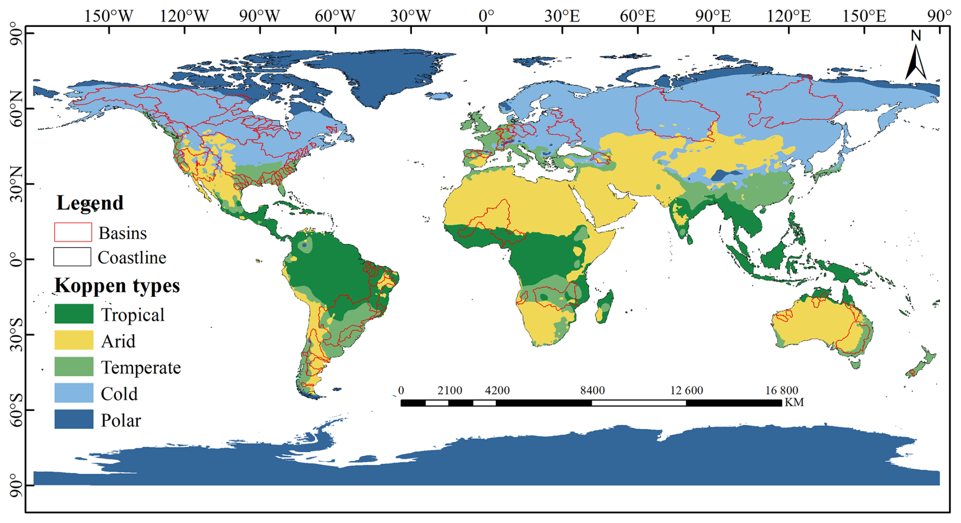
Figure 1 Overview of the Study Area. The climate classification used in this study is based on the Köppen climate classification system.

The climate classifications presented in Fig. 1 were determined using the Köppen climate classification system, a widely adopted framework that categorizes global climates based on temperature and precipitation thresholds (Crosbie et al., 2012; Hansford et al., 2020; Liu et al., 2022; Papacharalampous et al., 2023). This system divides the world into five primary climate types – Tropical, Arid, Temperate, Cold, and Polar. Its key strength lies in its integration of climate data with vegetation distribution, making it highly relevant to ecological environments.

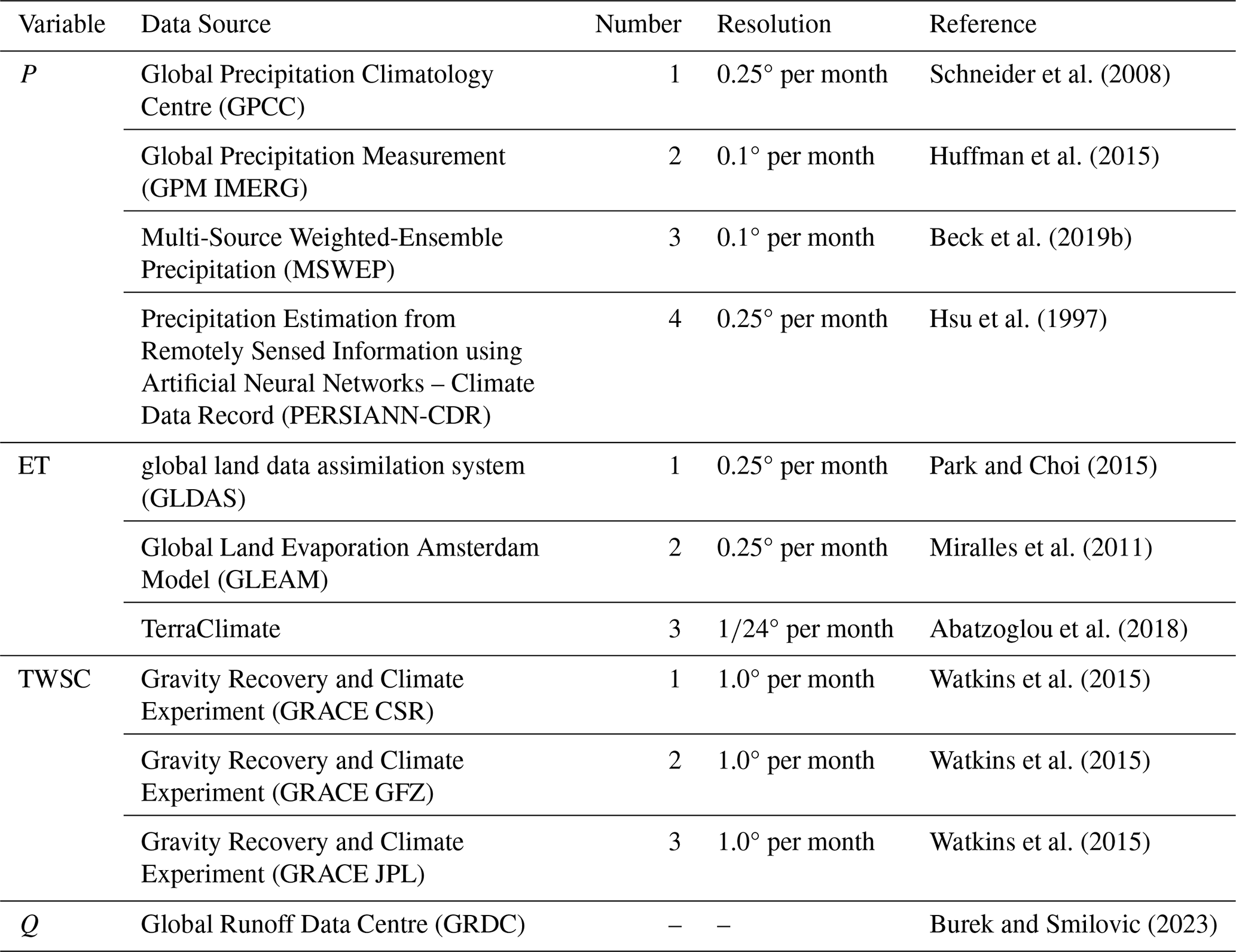
For each budget component, multiple datasets are typically available, with accuracy varying across different basins. No single dataset consistently performs best across all global basins. Therefore, multiple datasets were selected for each budget component to generate various data combinations (Eqs. 2–3). This approach ensures the inclusion of the most suitable dataset combinations while mitigating uncertainties associated with reliance on a single dataset.

Given the biases in the outputs of global P and ET models, observationally constrained datasets that have undergone bias correction or rigorous quality control are generally considered more accurate and reliable (Ehret et al., 2012). Accordingly, priority was given to datasets that incorporate extensive ground-based observations and provide bias-corrected or quality-controlled products. We selected four P datasets – GPCC, GPM IMERG, MSWEP, and PERSIANN-CDR; three ET datasets – GLDAS, GLEAM, and TerraClimate; and three TWSC datasets derived from GRACE satellite observations – GRACE CSR, GRACE GFZ, and GRACE JPL. All datasets were either bias-corrected according to the standards of their respective data providers or subjected to systematic quality control. Observed Q data were obtained from the GRDC platform. The above datasets were upscaled to the basin and monthly scales using spatial and temporal averaging. By combining these datasets, a total of 36 distinct data combinations were generated for each basin (Eq. 3).

$$\begin{array}{}\text{(2)}& C_{jkl}=\left[P_j{\text{ET}}_k{\text{TWSC}}_{l}Q\right]\end{array}$$

where j, k, and l represent the indices of the datasets corresponding to each budget component. Table 1 provides basic information on the datasets used in this study, along with their corresponding indices. Equation (3) represents a matrix composed of the elements defined in Eq. (2).

$$\begin{array}{}\text{(3)}& C=\left[\begin{array}{lllllllll}{C}_{\mathrm{111}}& C_{\mathrm{112}}& C_{\mathrm{113}}& C_{\mathrm{121}}& C_{\mathrm{122}}& C_{\mathrm{123}}& C_{\mathrm{131}}& C_{\mathrm{132}}& C_{\mathrm{133}}\\ C_{\mathrm{211}}& C_{\mathrm{212}}& C_{\mathrm{213}}& C_{\mathrm{221}}& C_{\mathrm{222}}& C_{\mathrm{223}}& C_{\mathrm{231}}& C_{\mathrm{232}}& C_{\mathrm{233}}\\ C_{\mathrm{311}}& C_{\mathrm{312}}& C_{\mathrm{313}}& C_{\mathrm{321}}& C_{\mathrm{322}}& C_{\mathrm{323}}& C_{\mathrm{331}}& C_{\mathrm{332}}& C_{\mathrm{333}}\\ C_{\mathrm{411}}& C_{\mathrm{412}}& C_{\mathrm{413}}& C_{\mathrm{421}}& C_{\mathrm{422}}& C_{\mathrm{423}}& C_{\mathrm{431}}& C_{\mathrm{432}}& C_{\mathrm{433}}\end{array}\right]\end{array}$$

The Global Precipitation Climatology Centre (GPCC) dataset, provided by the German Weather Service (DWD), is derived from a dense global network of rain gauge observations, and incorporates strict quality control procedures such as station data validation, temporal consistency checks, and outlier removal (Becker et al., 2013; Schneider et al., 2008). The dataset is available at 0.25° spatial resolution and daily to monthly temporal scales. The Global Precipitation Measurement Integrated Multi-Satellite Retrievals (GPM IMERG) Final Run product, developed by NASA and JAXA, integrates multiple satellite-based precipitation estimates and applies monthly bias correction using ground-based gauge data (Wang et al., 2017; Cui et al., 2020; Huang et al., 2019). The Multi-Source Weighted-Ensemble Precipitation (MSWEP) dataset combines satellite, gauge, and reanalysis data using an ensemble-weighted approach, incorporating over 77,000 ground stations for daily-scale bias correction (Beck et al., 2019a, 2017). The PERSIANN-CDR dataset, based on satellite remote sensing and artificial neural network technology, spans 60° S to 60° N with 0.25° daily resolution, and is bias-corrected using the GPCP monthly product, which includes extensive rain gauge observations (Chen et al., 2020b; Kaprom et al., 2025; Sadeghi et al., 2019).

For ET, the Global Land Data Assimilation System (GLDAS), developed by NASA and NOAA, uses land surface modeling and data assimilation to produce physically consistent estimates of land surface fluxes. The GLEAM dataset, developed by the Miralles team at the University of Bristol, estimates actual ET using satellite-derived net radiation and air temperature via the Priestley-Taylor model, and applies a stress factor derived from vegetation optical depth (VOD) and soil moisture to adjust potential evaporation. TerraClimate dataset provides global monthly actual ET estimates based on the Penman Montieth approach (Abatzoglou et al., 2018). Notably, bias correction in global ET products is generally less systematic than for P products, mainly due to the limited availability and spatial coverage of in situ flux tower observations. As a result, bias adjustments in ET datasets are typically indirect, relying on corrections applied to the climate forcing variables rather than to ET itself.

The launch of the GRACE and GRACE Follow-On (GRACE-FO) satellite missions has provided new opportunities for more accurate observations of large-scale TWSC. GRACE operated from 2002 to 2017, followed by GRACE-FO starting in 2018 (Boergens et al., 2024). These missions infer terrestrial total TWSC by tracking temporal variations in Earth's gravity field, which are primarily attributed to changes in terrestrial water mass. The GRACE TWSC datasets used in this study are provided by the University of Texas Center for Space Research (CSR), the German Research Centre for Geosciences (GFZ), and NASA's Jet Propulsion Laboratory (JPL), all of which include multiple bias correction procedures to improve data quality (Landerer et al., 2012; Shamsudduha et al., 2017). These bias correction procedures include filtration to suppress correlated noise and striping artifacts (Swenson and Wahr, 2006), replacement of poorly resolved spherical harmonic coefficients (e.g., degree-2 term C20) with satellite laser ranging data (Loomis et al., 2020), and correction for glacial isostatic adjustment (GIA) (Peltier et al., 2012; Mu et al., 2017). Numerous studies have demonstrated the sensitivity and reliability of GRACE satellite data for monitoring TWSC (Swenson and Wahr, 2006; Resende et al., 2019; Majid et al., 2019; Reager et al., 2014).

The GRDC provides the most comprehensive open-access river discharge data available worldwide, collected from national hydrological agencies. This dataset includes river streamflow measurements from over 10 000 stations across 159 countries (Su and Zhang, 2024). To minimize the impact of missing data on the reliability of the results, hydrological stations were selected based on the criterion that missing values accounted for less than 10 % of the total dataset. Linear interpolation was then applied to fill any remaining data gaps.

Table 1 Datasets used for this study.

3 Methods

3.1 Water imbalance error

The water balance equation describes the conservation of mass between water inflows, outflows, and changes in storage within a given region (Eq. 1). However, in practice, this balance is rarely achieved due to various sources of error. These include systematic biases (such as missed portions of outflow resulted from unclosed basin boundaries and inaccuracies in catchment area delineation, particularly in small basins), measurement uncertainties, and the omission of unmeasured components. Consequently, each budget component (P, ET, Q, and TWSC) is subject to an associated error term (denoted as ε_P, ε_ET, ε_Q, ε_TWSC, respectively), leading to a non-closure of the water budget (i.e., Eq. 1 becomes Eq. 4) (Aires, 2014; Wong et al., 2021). The resulting imbalance is represented by the residual error term ΔRes (Eq. 5), which quantifies the inconsistency among the observed or estimated components of the water cycle.

Minimizing the ΔRes error is a key objective in practical hydrological applications, as it enhances the accuracy and reliability of budget component datasets. However, it is important to note that smaller ΔRes values may arise from error compensation among budget components rather than genuine improvements in data accuracy. Therefore, a high-precision water balance dataset is characterized not only by a near-zero ΔRes error but also by budget components that closely approximate their true values (Luo et al., 2023a).

$$\begin{array}{}\text{(4)}& {\displaystyle }\begin{array}{rl}\left(P+{\mathit{\epsilon }}_P\right)& -\left(\mathrm{ET}+{\mathit{\epsilon }}_{\mathrm{ET}}\right)-\left(Q+{\mathit{\epsilon }}_Q\right)\\ & -\left(\mathrm{TWSC}+{\mathit{\epsilon }}_{\mathrm{TWSC}}\right)=\mathrm{0}\end{array}\text{(5)}& {\displaystyle }\begin{array}{rl}\mathrm{\Delta }\mathrm{Res}& ={\mathit{\epsilon }}_{\mathrm{ET}}+{\mathit{\epsilon }}_Q+{\mathit{\epsilon }}_{\mathrm{TWSC}}-{\mathit{\epsilon }}_P\\ & =P-\text{ET}-Q-\text{TWSC}\end{array}\end{array}$$

where ε_P, ε_ET, ε_Q, ε_TWSC are the errors in budget components of P, ET, Q, and TWSC relative to their true values, respectively.

3.2 Existing water budget closure correction methods

To minimize the ΔRes error in Eq. (5) (reducing ΔRes from ≠0 to 0), various statistical BCC methods have been developed. These methods differ in their principles for redistributing the ΔRes error, leading to varying levels of introduced uncertainty. To systematically assess the uncertainties associated with existing BCC methods in closing the water budget and to reduce uncertainty in method selection, we evaluated four representative methods: PR, CKF, MCL, and MSD (Luo et al., 2023b; Abolafia-Rosenzweig et al., 2021; Dastjerdi et al., 2024). In the following application of these BCC methods, the TWSC data used in this study refer to the basin-scale total terrestrial water storage change observed by GRACE satellite data.

For each basin, these four methods were applied to 36 different data combinations (Eq. 3), yielding 144 uncertainty estimates. The optimal combinations were identified using a 5 % threshold. By averaging the errors introduced into budget components across these selected optimal combinations, we quantified the uncertainty associated with existing BCC methods. This approach minimizes uncertainties arising from both BCC method selection and budget component data selection, enabling a more objective evaluation of the errors introduced by existing BCC methods. A brief overview of the four BCC methods is provided below:

1. PR method.

   The PR method assumes that the error in budget components is proportional to their magnitudes (Abatzoglou et al., 2018). Based on the relative magnitudes of these variables, the ΔRes error is redistributed across them to achieve water budget closure (Eq. 6).

   $$\begin{array}{}\text{(6)}& F_i=X_i-\mathrm{\Delta }\text{Res}\left(G_i\right)\left({\displaystyle \frac{\mathrm{|}{X}_i\mathrm{|}}{{\sum }_{j=\mathrm{1}}^n\mathrm{|}{X}_j\mathrm{|}}}\right)\end{array}$$

   where F_i and X_i represent the corrected and original data for budget components (P, ET, Q and TWSC), respectively; n denotes the number of budget components involved in the water budget closure calculation; ΔRes represents the water imbalance error; G is a constant vector defined as $G=[\mathrm{1}-\mathrm{1}-\mathrm{1}-\mathrm{1}]$.

2. CKF method.

   The CKF method is developed based on the Kalman filter method (Pan and wood, 2006). For a given set of estimated budget components X=[P ET Q TWSC]^T and their estimated errors $\mathrm{\Delta }\text{Res}=\mathit{G}X\ne \mathrm{0}$ (where G is a constant vector, $G=[\mathrm{1}-\mathrm{1}-\mathrm{1}-\mathrm{1}])$, the goal is to find a new set of estimates $F=[P^{\prime }{\text{ET}}^{\prime }{Q}^{\prime }{\text{TWSC}}^{\prime }{]}^T$ such that $\mathit{G}{X}^{\prime }=\mathrm{0}$, achieving water budget closure (Pan et al., 2012). In simple terms, the CKF method redistributes the ΔRes among the budget components based on the error covariance of X, defined as Δε_XX (Eq. 7), to obtain a closured dataset.

   $$\begin{array}{}\text{(7)}& \mathrm{\Delta }{\mathit{\epsilon }}_{XX}=\stackrel{\mathrm{‾}}{(X-X_{\mathrm{0}})(X-X_{\mathrm{0}}{)}^T}\end{array}$$

   where X₀ refers to the reference values of the estimated budget components, and the bar over an expression denotes expectation. For P, ET and TWSC, the reference values X₀ were calculated by averaging all considered datasets, following previous studies (Zhang et al., 2018; Abolafia-Rosenzweig et al., 2021). For Q, we adopted observed Q. Due to the difficulty in quantifying the uncertainty in observed Q, previous studies have reported gauge-based uncertainty as a percent error for some of the basins, ranging from 2.3 %–28.8 % (Clarke, 1999; Mueller, 2003; Shiklomanov et al., 2006; Abolafia-Rosenzweig et al., 2021). We followed a similar approach to estimate the uncertainty associated with Q in this study.

   The error covariance matrix Δε_XX is of dimension 4×4 and represents the covariances among errors in the four budget components:

   $$\begin{array}{}\text{(8)}& \mathrm{\Delta }{\mathit{\epsilon }}_{XX}=\left[\begin{array}{llll}\mathrm{\Delta }{\mathit{\epsilon }}_{P-P}& \mathrm{\Delta }{\mathit{\epsilon }}_{P-\mathrm{ET}}& \mathrm{\Delta }{\mathit{\epsilon }}_{P-Q}& \mathrm{\Delta }{\mathit{\epsilon }}_{P-\mathrm{TWSC}}\\ \mathrm{\Delta }{\mathit{\epsilon }}_{\mathrm{ET}-P}& \mathrm{\Delta }{\mathit{\epsilon }}_{\mathrm{ET}-\mathrm{ET}}& \mathrm{\Delta }{\mathit{\epsilon }}_{\mathrm{ET}-Q}& \mathrm{\Delta }{\mathit{\epsilon }}_{\mathrm{ET}-\mathrm{TWSC}}\\ \mathrm{\Delta }{\mathit{\epsilon }}_{Q-P}& \mathrm{\Delta }{\mathit{\epsilon }}_{Q-\mathrm{ET}}& \mathrm{\Delta }{\mathit{\epsilon }}_{Q-Q}& \mathrm{\Delta }{\mathit{\epsilon }}_{Q-\mathrm{TWSC}}\\ \mathrm{\Delta }{\mathit{\epsilon }}_{\mathrm{TWSC}-P}& \mathrm{\Delta }{\mathit{\epsilon }}_{\mathrm{TWSC}-\mathrm{ET}}& \mathrm{\Delta }{\mathit{\epsilon }}_{\mathrm{TWSC}-Q}& \mathrm{\Delta }{\mathit{\epsilon }}_{\mathrm{TWSC}-\mathrm{TWSC}}\end{array}\right]\end{array}$$

   Following Pan et al. (2012), the off-diagonal elements representing cross-variable error covariances were assumed to be zero, under the assumption that errors among different budget components are uncorrelated. Accordingly, the matrix F can be computed as shown in Eq. (9).

   $$\begin{array}{}\text{(9)}& \mathbf{F}=X+K(\mathrm{0}-\mathit{G}X)\end{array}$$

   where $K=\mathrm{\Delta }{\mathit{\epsilon }}_{XX}{C}^T(C\mathrm{\Delta }{\mathit{\epsilon }}_{XX}{C}^T{)}^{-\mathrm{1}}$ is the Kalman gain. Setting GX=ΔRes, and Eq. (9) can be rewritten as Eq. (10).

   $$\begin{array}{}\text{(10)}& \mathbf{F}=X-\mathrm{\Delta }{\mathit{\epsilon }}_{XX}{G}^T(\mathit{G}\mathrm{\Delta }{\mathit{\epsilon }}_{XX}{G}^T{)}^{-\mathrm{1}}\mathrm{\Delta }\text{Res}\end{array}$$

   where error covariance ε_XX is calculated entry by entry according to Eq. (8).

3. MCL method.

   The MCL method is an extension of the triple collocation (TC) method. It calculates the weights for redistributing the ΔRes error among budget components by estimating the errors relative to their true values (expressed as distances, without requiring knowledge of the true values). The fundamental equations of the MCL method are shown in Eqs. (11)–(12).

   $$\begin{array}{}\text{(11)}& {\displaystyle }{F}_i=X_i-\mathrm{\Delta }\text{Res}\left(G^i\right)\left(d_{x{x}_{\mathrm{0}}-\text{norm}}^i\right)\text{(12)}& {\displaystyle }{d}_{x{x}_{\mathrm{0}}-\text{norm}}^i={\displaystyle \frac{d_{x{x}_{\mathrm{0}}}^i}{\sum _{j=\mathrm{1}}^{\mathrm{4}}\left|d_{x{x}_{\mathrm{0}}}^j\right|}}\end{array}$$

   In these equations, F_i represents the corrected data for the ith budget component; X_i denotes the original data for the ith budget component; ΔRes represents the water imbalance error; $d_{x{x}_{\mathrm{0}}-\text{norm}}^i$ represents the weight assigned to the ith budget component, and $d_{x{x}_{\mathrm{0}}}^i$ represents the distance between the ith budget component and the true value, as calculated using the Monte Carlo (MC) method. For example, in the case of five precipitation data products (N=5), the calculation of $d_{x{x}_{\mathrm{0}}}^i$ (d1t, d2t, d3t, d4t, and d5t) is shown in Eqs. (13)–(14).

   $$\begin{array}{}\text{(13)}& {\displaystyle }{A}_{\left(N\right)}{y}_{\left(N\right)}=b_{\left(N\right)}\text{(14)}& {\displaystyle }\begin{array}{rl}& A_{\left(\mathrm{5}\right)}=\left[\begin{array}{lllll}\mathrm{1}& \mathrm{1}& \mathrm{0}& \mathrm{0}& \mathrm{0}\\ \mathrm{1}& \mathrm{0}& \mathrm{1}& \mathrm{0}& \mathrm{0}\\ \mathrm{1}& \mathrm{0}& \mathrm{0}& \mathrm{1}& \mathrm{0}\\ \mathrm{1}& \mathrm{0}& \mathrm{0}& \mathrm{0}& \mathrm{1}\\ \mathrm{0}& \mathrm{1}& \mathrm{1}& \mathrm{0}& \mathrm{0}\\ \mathrm{0}& \mathrm{1}& \mathrm{0}& \mathrm{1}& \mathrm{0}\\ \mathrm{0}& \mathrm{1}& \mathrm{0}& \mathrm{0}& \mathrm{1}\\ \mathrm{0}& \mathrm{0}& \mathrm{1}& \mathrm{1}& \mathrm{0}\\ \mathrm{0}& \mathrm{0}& \mathrm{1}& \mathrm{0}& \mathrm{1}\\ \mathrm{0}& \mathrm{0}& \mathrm{0}& \mathrm{1}& \mathrm{1}\end{array}\right],\\ & y_{\left(\mathrm{5}\right)}=\left[\begin{array}{l}{d}_{\mathrm{1}t}^{\mathrm{2}}\\ d_{\mathrm{2}t}^{\mathrm{2}}\\ d_{\mathrm{3}t}^{\mathrm{2}}\\ d_{\mathrm{4}t}^{\mathrm{2}}\\ d_{\mathrm{5}t}^{\mathrm{2}}\end{array}\right],b_{\left(\mathrm{5}\right)}=\left[\begin{array}{l}{d}_{\mathrm{12}}^{\mathrm{2}}\\ d_{\mathrm{13}}^{\mathrm{2}}\\ d_{\mathrm{14}}^{\mathrm{2}}\\ d_{\mathrm{15}}^{\mathrm{2}}\\ d_{\mathrm{23}}^{\mathrm{2}}\\ d_{\mathrm{24}}^{\mathrm{2}}\\ d_{\mathrm{25}}^{\mathrm{2}}\\ d_{\mathrm{34}}^{\mathrm{2}}\\ d_{\mathrm{35}}^{\mathrm{2}}\\ d_{\mathrm{45}}^{\mathrm{2}}\end{array}\right]\end{array}\end{array}$$

4. MSD method.

   The MSD method redistributes the ΔRes to each budget component based on minimizing the time-series deviation error, aiming to reduce model uncertainties caused by errors in estimating time-point deviations (Luo et al., 2023b). Specifically, the MSD method first calculates the minimum time-series deviation distance between remote sensing data for budget components and multi-source integrated data products (EO) (Eq. 15).

   $$\begin{array}{}\text{(15)}& \begin{array}{rl}{D}_{x,\to n}& =-{\displaystyle \frac{{\left[{\sum }_{j=\mathrm{1}}^n(y_{(\text{EO},j)}-\stackrel{\mathrm{‾}}{y_{(\text{EO},\to n)}})(x_{(\text{RS},j)}-\stackrel{\mathrm{‾}}{x_{(\text{RS},\to n)}})\right]}^{\mathrm{2}}}{{\sum }_{j=\mathrm{1}}^n(x_{(\text{RS},j)}-\stackrel{\mathrm{‾}}{x_{(\text{RS},\to n)}}{)}^{\mathrm{2}}}}\\ & +{\sum }_{j=\mathrm{1}}^n(y_{(\text{EO},j)}-\stackrel{\mathrm{‾}}{y_{(\text{EO},\to n)}}{)}^{\mathrm{2}}\end{array}\end{array}$$

   where $D_{x,\to n}$ represents the minimum time-series deviation distance for budget component x (e.g., P, ET, TWSC); y_(EO,j) and x_(RS,j) refer to the integrated value and raw value of the budget component x, respectively; $\stackrel{\mathrm{‾}}{y_{(\text{EO},\to n)}}$ and $\stackrel{\mathrm{‾}}{x_{(\text{RS},\to n)}}$ denote the average deviation of budget component x from the first to the nth time point.

   Next, the MSD method calculates the weights for each budget component based on $D_{x,\to n}$ (Eq. 16).

   $$\begin{array}{}\text{(16)}& w_{x,j}={\displaystyle \frac{D_{x,\to j}}{{\sum }_{i=\mathrm{1}}^{\mathrm{4}}{D}_{i,\to j}}}\end{array}$$

   where w_x,j is the weight of budget component x at time point j.

   Finally, the weight calculation results from Eq. (16) are substituted into Eq. (17) to achieve water budget closure.

   $$\begin{array}{}\text{(17)}& \begin{array}{rl}\left[\begin{array}{l}{F}_{P,j}^{\mathrm{BCC}}\\ F_{\mathrm{ET},j}^{\mathrm{BCC}}\\ F_{R,j}^{\mathrm{BCC}}\\ F_{\mathrm{TWSC},j}^{\mathrm{BCC}}\end{array}\right]& =\left[\begin{array}{l}{F}_{P,j}^{\mathrm{Raw}}\\ F_{\mathrm{ET},j}^{\mathrm{Raw}}\\ F_{R,j}^{\mathrm{Raw}}\\ F_{\mathrm{TWSC},j}^{\mathrm{Raw}}\end{array}\right]\\ & -\mathrm{\Delta }\text{Res}\left[\begin{array}{r}\mathrm{1}\\ -\mathrm{1}\\ -\mathrm{1}\\ -\mathrm{1}\end{array}\right]\left[\begin{array}{l}{w}_{P,j}\\ w_{\mathrm{ET},j}\\ w_{R,j}\\ w_{\mathrm{TWSC},j}\end{array}\right]\end{array}\end{array}$$

   where F^BCC represents the budget components (P, ET, Q, and TWSC) corrected for water budget closure, while F^Raw denotes the raw, uncorrected values of the budget components.

3.3 Uncertainties introduced by existing BCC methods for closing water budget

When the existing BCC methods described in Sect. 3.2 are applied to close the water budget, they redistribute ΔRes based on the estimated errors of budget components but neglect unmeasured components. This inevitably leads to an unreasonable redistribution of the ΔRes error, introducing new uncertainties. The magnitude of these introduced errors and whether they can be ignored remain unresolved, primarily due to insufficient observational data for some budget components, making it difficult to quantify the associated uncertainties.

Our analysis in this study reveals that when existing BCC methods are used for water budget closure, certain budget components that typically have positive values, such as P, ET, and Q, occasionally become negative in some months. Previous studies have also mentioned this issue (Lehmann et al., 2022). This clearly indicates an unreasonable redistribution of ΔRes errors, underscoring the urgent need for methodological improvements. Despite this issue, research on negative values remains limited. Key questions persist regarding the proportion of negative values in each budget component under current BCC methods, which variables are most susceptible to severe negative values, and how these errors vary throughout the year. Addressing these questions is critical for refining existing BCC methods.

Notably, quantifying negative values does not require observational data. To comprehensively assess the uncertainties introduced by forced water budget closure, we consider three aspects: errors of individual budget components relative to observed values (Sect. 4.2.1), negative values arising from budget closure (Sect. 4.2.2), and ensemble errors (Sect. 4.2.3).

1. Errors of individual budget components.

   Quantifying this type of error requires determining reference values for budget components. However, for certain variables, such as ET, observational data are insufficient across global watersheds, posing a major challenge in accurately characterizing global ET patterns. As a result, approximate reference values must be used to ensure the reliability of the results.

   In this study, reference values for budget components were established based on the following principles. For Q, long-term observational records from hydrological stations were available for all selected basins, meeting the study's requirements. For TWSC, we utilized three observational datasets from the GRACE satellite, which currently provides the only large-scale measurements of basin water storage changes under rigorous quality control. The reliability of GRACE data has been validated through ground-based observations (Famiglietti et al., 2011; Landerer et al., 2020; Rodell et al., 2009; Tapley et al., 2004; Yeh et al., 2006). Thus, GRACE TWSC data can be considered approximately reliable. To further enhance its accuracy, we applied data fusion techniques, as described in Eq. (18), to merge the three GRACE TWSC products into a single reference dataset (Munier and Aires, 2018; Zhang et al., 2018).

   The uncertainty introduced by existing BCC methods for precipitation was evaluated from two perspectives. First, 13 basins with sufficient observational precipitation data were selected, using observed precipitation as the reference. This sample size was sufficient for assessing the uncertainties associated with existing BCC methods. Second, 71 additional basins lacking sufficient observational precipitation data were included, for which fused precipitation values, derived using Eq. (18), served as reference. This approach enabled cross-validation of the reliability of the fused dataset by comparing results with those from basins with observational data, allowing the study to be extended to a larger number of basins.

   ET is the most challenging budget component to measure directly. The scarcity of globally available ET observational data precludes the direct use of observed ET as a reference. To address this limitation, previous studies have either focused on a few basins with available observational data or compared multiple existing ET datasets. ET products are generally considered reliable if their magnitudes and trends align with those of other datasets (Chen et al., 2021; Pan et al., 2020; Xu et al., 2019). Some studies have also employed the fusion of multiple data products as a reference for ET validation (Jiménez et al., 2018; Mueller et al., 2011; Yao et al., 2014). Following this approach, we assessed the uncertainty introduced by existing BCC methods for ET by utilizing a fusion-based reference dataset.

   $$\begin{array}{}\text{(18)}& \stackrel{\mathrm{‾}}{M_x}={\sum }_{i=\mathrm{1}}^n{M}_{x,i}\cdot {\mathit{\omega }}_i\text{ and }{\mathit{\omega }}_i={\displaystyle \frac{\mathrm{1}}{{\mathit{\sigma }}_i^{\mathrm{2}}}}/{\sum }_{i=\mathrm{1}}^{\mathrm{1}}{\displaystyle \frac{\mathrm{1}}{{\mathit{\sigma }}_i^{\mathrm{2}}}}\end{array}$$

   where $\stackrel{\mathrm{‾}}{M_x}$ represents the fused value of the budget component, M_x,i denotes the ith product of the budget component; ω_i denotes the weight of the ith product, and ${\mathit{\sigma }}_i^{\mathrm{2}}$ refers to the covariance error of the ith product, n is the total number of budget components, and x refers to P, ET or TWSC.

   After establishing reference values for budget components, we quantify errors in the original data relative to these references, using the positive metric CC and inverse metric RMSE as examples, denoted as CC₁ and RMSE₁, respectively. Similarly, errors in the BCC-corrected data relative to the reference values are calculated, represented as CC₂ and RMSE₂.

   To assess the uncertainties introduced by water budget closure, changes in CC and RMSE (CC^′ and RMSE^′) are computed using Eqs. (19) and (22). Positive values of CC^′ and RMSE^′ indicate an improvement in data accuracy following BCC correction, whereas negative values suggest a decline. In addition to CC and RMSE, other statistical metrics used in this study include the positive indicator NSE and the negative indicator MAE.

   $$\begin{array}{}\text{(19)}& {\displaystyle }{\mathrm{CC}}^{\prime }={\text{CC}}_{\mathrm{2}}-{\text{CC}}_{\mathrm{1}}\text{(20)}& {\displaystyle }{\text{NSE}}^{\prime }={\text{NSE}}_{\mathrm{2}}-{\text{NSE}}_{\mathrm{1}}\text{(21)}& {\displaystyle }{\text{MAE}}^{\prime }={\text{MAE}}_{\mathrm{1}}-{\text{MAE}}_{\mathrm{2}}\text{(22)}& {\displaystyle }{\text{RMSE}}^{\prime }={\text{RMSE}}_{\mathrm{1}}-{\text{RMSE}}_{\mathrm{2}}\text{(23)}& {\displaystyle }\mathrm{\text{CC}}={\displaystyle \frac{{\sum }_{i=\mathrm{1}}^n({\text{Obs}}_i-\stackrel{\mathrm{‾}}{\text{Obs}})({\text{Sim}}_i-\stackrel{\mathrm{‾}}{\text{Sim}})}{\sqrt{{\sum }_{i=\mathrm{1}}^n({\text{Obs}}_i-\stackrel{\mathrm{‾}}{\text{Obs}}{)}^{\mathrm{2}}}\sqrt{{\sum }_{i=\mathrm{1}}^n({\text{Sim}}_i-\stackrel{\mathrm{‾}}{\text{Sim}}{)}^{\mathrm{2}}}}}\text{(24)}& {\displaystyle }\text{NSE}=\mathrm{1}-{\displaystyle \frac{{\sum }_{i=\mathrm{1}}^n({\text{Sim}}_i-{\text{Obs}}_i{)}^{\mathrm{2}}}{{\sum }_{i=\mathrm{1}}^n({\text{Obs}}_i-\stackrel{\mathrm{‾}}{\text{Obs}}{)}^{\mathrm{2}}}}\text{(25)}& {\displaystyle }\text{MAE}={\displaystyle \frac{\mathrm{1}}{n}}{\sum }_{i=\mathrm{1}}^n\left|{\text{Sim}}_i-{\text{Obs}}_i\right|\text{(26)}& {\displaystyle }\text{RMSE}=\sqrt{{\displaystyle \frac{\mathrm{1}}{n}}{\sum }_{i=\mathrm{1}}^n({\text{Obs}}_i-{\text{Sim}}_i{)}^{\mathrm{2}}}\end{array}$$

   where Obs_i represents the reference value at time i, and Sim_i represents either the original data or the BCC-corrected data. $\stackrel{\mathrm{‾}}{\text{Obs}}$ and $\stackrel{\mathrm{‾}}{\text{Sim}}$ represent the mean values of Obs and Sim, respectively, and n is the sample size.

2. Negative values.

   Negative values are defined as the issue that arises when the BCC method is used to close the water budget, and the redistributed ΔRes error exceeds the actual values of budget components (P, ET, Q, and TWSC), causing P, ET, and Q to become negative. For TWSC, a negative value occurs when the corrected TWSC has an opposite sign to its raw value. These negative values represent only a subset of the errors introduced during water budget closure but reflect an extreme case of unreasonable ΔRes error redistribution, serving as an indicator of the BCC method's effectiveness.

   When a budget component exhibits a negative value, the redistribution of ΔRes errors to other components is significantly affected, reducing the overall accuracy of the corrected datasets. Thus, negative values are a critical factor influencing the performance of existing BCC methods and should be prioritized for improvement. To better understand this issue, we analyze the proportion of negative values for each budget component, their seasonal distribution, and their sensitivity to climatic conditions (i.e., their prevalence in arid versus humid basins). Insights from this analysis were incorporated into the proposed IWE-Res method to address the occurrence of negative values (Sect. 3.4).

3. Ensembled error of four budget components.

   The aforementioned evaluations (1) and (2) assess errors for individual budget components. To gain a more comprehensive understanding of the uncertainties introduced by water budget closure, we also evaluate the combined error. First, the absolute error (AE) of each budget component is calculated (using P as an example, see Eq. 29). Second, the relative absolute error (RAE) is determined for each budget component (Eq. 28). Finally, by aggregating the relative errors of individual components, we define the ensembled relative error (Eq. 27) to quantify the overall error introduced by BCC methods.

   $$\begin{array}{}\text{(27)}& {\displaystyle }\begin{array}{rl}F\left(\text{Re}\right)& ={\displaystyle \frac{\mathrm{1}}{n}}{\sum }_{i=\mathrm{1}}^n{\displaystyle \frac{\begin{array}{c}\left|\text{AE}\left(P^{\prime }\right)\right|-\left|\text{AE}\left(P_{\mathrm{Raw}}\right)\right|+\left|\text{AE}\left({\text{ET}}^{\prime }\right)\right|\\ -\left|\text{AE}\left({\text{ET}}_{\mathrm{Raw}}\right)\right|+\left|\text{AE}\left(Q^{\prime }\right)\right|\\ -\left|\text{AE}\left(Q_{\mathrm{Raw}}\right)\right|+\left|\text{AE}\left({\text{TWSC}}^{\prime }\right)\right|\\ -\left|\text{AE}\left({\text{TWSC}}_{\mathrm{Raw}}\right)\right|\end{array}}{P_{\mathrm{0}}+{\text{ET}}_{\mathrm{0}}+Q_{\mathrm{0}}+\left|{\text{TWSC}}_{\mathrm{0}}\right|}}\\ & ={\displaystyle \frac{\mathrm{1}}{n}}\sum _{i=\mathrm{1}}^n{\displaystyle \frac{\text{RAE}\left(P\right)+\text{RAE}\left(\text{ET}\right)+\text{RAE}\left(Q\right)+\text{RAE}\left(\text{TWSC}\right)}{P_{\mathrm{0}}+{\text{ET}}_{\mathrm{0}}+Q_{\mathrm{0}}+\left|{\text{TWSC}}_{\mathrm{0}}\right|}}\end{array}\text{(28)}& {\displaystyle }\text{RAE}\left(P\right)=\left|\text{AE}\left(P^{\prime }\right)\right|-\left|\text{AE}\left(P_{\mathrm{Raw}}\right)\right|\text{(29)}& {\displaystyle }\text{AE}\left(P\right)=\left|P-P_{\mathrm{0}}\right|\end{array}$$

   where, F(Re) represents the ensembled relative error, and RAE refers to the relative value of absolute error, with i denoting the month. The subscript “Raw” corresponds to the raw data of the budget components, the subscript 0 represents the observed data, the superscript “^′” denotes the BCC-corrected data for the budget components. The degree of alteration induced by the BCC methods for each budget component are defined based on the value of F(Re), and four intervals are established in 5 % increments: no significant change [0 %–5 %], minor change (5 %–10 %], moderate change (10 %–15 %], and significant change (>15 %).

3.4 Proposed IWE-Res method for closing water budget

In this section, we propose the IWE-Res method to identify the optimal balance for redistributing ΔRes, minimizing the sum of the introduced error to budget components and the remaining ΔRes error while reducing the negative values introduced by closing the water budget. Unlike existing BCC methods that fully redistribute the ΔRes term in a single step, the IWE-Res method adopts a gradual, iterative redistribution strategy that allows for more consistent correction. Specifically, the method incrementally allocates fractions of ΔRes to P, ET, Q and TWSC, based on fixed percentage steps and guided by existing BCC weighting schemes. At each iteration, the redistribution process seeks to minimize the combined error – defined as the sum of the induced changes in the water budget components and the remaining unexplained ΔRes. This dual-objective criterion ensures that the method balances error reduction while maintaining hydrological plausibility. Importantly, the approach includes a mechanism to avoid introducing implausible negative values. If, during any iteration, the corrected value of a component becomes negative – violating hydrological constraints such as non-negative precipitation or runoff – further redistribution to that component is halted. Subsequent iterations reallocate the remaining ΔRes among the unaffected components. From a hydrological perspective, this strategy acknowledges that not all of the residuals can be attributed to known components. Some portion of ΔRes may originate from unmeasured or poorly constrained processes. By partially closing the water budget in a controlled and iterative manner, the IWE-Res method reduces the risk of overcorrecting well-characterized components while better preserving the consistency of the entire budget. The specific steps of the proposed IWE-Res method are as follows:

First, the ΔRes error is calculated using Eq. (5) and the original datasets of budget components.

Second, an iterative loop is constructed to compute the errors introduced into budget components during the gradual redistribution of the ΔRes error and to address negative values. To more accurately identify the optimal balance, a step size of 0.1 % of ΔRes is used in each iteration in this study. We denote the ΔRes redistributed to budget components in each iteration as x, where $x\in [\mathrm{0},\mathrm{\Delta }\text{Res}]$.

During each redistribution of ΔRes, two error terms are computed: (1) the remaining ΔRes error, defined as ΔRes* =ΔRes − x, and (2) the error introduced to budget components due to the redistribution of the x error, denoted as IWE (Eq. 31). When these errors are plotted in a coordinate system, two distinct curves emerge (Fig. 2), each representing a different error relationship. For ΔRes* (Eq. 30), Fig. 2 shows a fixed, monotonically decreasing linear trend, as 0.1 % increments of ΔRes are uniformly redistributed to budget components using existing BCC methods. In contrast, the IWE curve exhibits a non-fixed shape, reflecting the cumulative error introduced to budget components during the redistribution of a portion of ΔRes (Eqs. 31–32). This variability in the IWE curve arises from the nonlinear relationship between the introduced budget component errors and the reduction in ΔRes error.

$$\begin{array}{}\text{(30)}& {\displaystyle }\mathrm{\Delta }{\text{Res}}^{*}=ax+b=-x+\mathrm{\Delta }\text{Res}\text{(31)}& {\displaystyle }\text{IWE}=F({\mathit{\epsilon }}_P,{\mathit{\epsilon }}_{\mathrm{ET}},{\mathit{\epsilon }}_Q,{\mathit{\epsilon }}_{\mathrm{TWSC}})=F(x,\text{RAE})\text{(32)}& {\displaystyle }\begin{array}{rl}\text{RAE}& ={\displaystyle \frac{\mathrm{1}}{\mathrm{4}}}\sum _{i=\mathrm{1}}^{\mathrm{4}}(\text{RAE}\left(P\right)\\ & +\text{RAE}\left(\text{ET}\right)+\text{RAE}\left(Q\right)+\text{RAE}\left(\text{TWSC}\right))\end{array}\end{array}$$

where x represents the portion of ΔRes redistributed to the budget components, with a range from 0 to ΔRes. The terms ε_P, ε_ET, ε_Q, ε_TWSC represent the errors introduced to P, ET, Q and TWSC, respectively, due to the redistribution of x to the budget components. F(x,RAE) denotes the RAE error calculated by the redistribution of the x error to budget components.

During the iterative correction process, if any of the water budget components (P, ET, and Q) becomes negative, the redistribution of water imbalance error to that component is immediately suspended. In subsequent iterations, redistribution is recalculated to ensure that only components with physically meaningful positive values receive the imbalance correction. For example, if ET becomes negative in a given iteration, the imbalance is subsequently redistributed to P, Q, and TWSC only, in accordance with Eq. (33). For TWSC, if a sign reversal occurs during iteration (i.e., from positive to negative or vice versa), the redistribution of the water imbalance error to TWSC is suspended in the following iteration.

$$\begin{array}{}\text{(33)}& F_i=X_i-x\left(G_i\right)\left({\displaystyle \frac{\left|{\mathit{\epsilon }}_i\right|}{{\sum }_{j=\mathrm{1}}^n\left|{\mathit{\epsilon }}_j\right|}}\right)\end{array}$$

where F_i denotes the corrected dataset, and X_i denotes the original dataset of budget components. Since ET does not participate in the redistribution of the residual error x based on the example above, the weighting vector is defined as $G=[\mathrm{1},\mathrm{0},-\mathrm{1},-\mathrm{1}]$. The term ε represents the error in budget components estimated using existing BCC methods, as described in Sect. 3.2.

Third, the IWE-Res curve is plotted (Fig. 2) to provide an intuitive comparison between the introduced budget component errors and the remaining water imbalance error. The error calculation results from Eqs. (30) and (31) are presented within the same coordinate system.

The IWE-Res method is illustrated in Fig. 2 using four curves. The x axis represents the percentage of water imbalance error redistributed to budget components using existing BCC methods, while the y axis denotes the percentage of the remaining water imbalance error (ΔRes*) after each iteration. The black dashed line represents the redistributed x-error value among the budget components. The thin blue solid line represents the ΔRes* error curve. Since the sum of redistributed x and remaining ΔRes* equals the total ΔRes error, this curve forms a monotonically decreasing 45° line. The thin green solid line represents the introduced budget component error (IWE) after a given percentage of ΔRes is redistributed (x axis), with its shape varying depending on the redistribution process (Fig. 2 is illustrative). Initially, when no ΔRes is redistributed (x=0), the IWE error is zero. As more ΔRes is redistributed (with increasing x values), IWE increases due to the growing uncertainty introduced. The thin red solid line represents the total error, defined as the sum of ΔRes* and IWE after applying BCC methods. This curve varies depending on the redistribution process, and its minimum value identifies the optimal balance where combined ΔRes* and IWE errors are minimized. The intersection of the ΔRes* and IWE curves indicates only the point at which these errors are equal, not necessarily the optimal balance.

To determine the optimal redistribution of the water imbalance error, we plot the IWE-Res curve (the green solid line) for each basin, identifying the minimum of the red total error curve. We then analyze its patterns across basins with different characteristics to optimize water budget closure and improve the accuracy of budget component datasets.

The IWE error in Fig. 2 also serves as a metric for evaluating the performance of existing BCC methods. If a BCC method perfectly redistributed ΔRes without introducing additional errors, the IWE curve would be a flat line at zero, and the red total error line would coincide with the blue ΔRes* error line. This scenario indicates that full redistribution of water imbalance error achieves the optimal balance, providing indirect validation of the IWE-Res method's effectiveness.

Finally, the optimal balance is identified, enabling the generation of a high-precision dataset that improves water budget closure. The optimal balance corresponds to the minimum of the total error curve (IWE + ΔRes*), where the sum of remaining water imbalance error and introduced budget component errors is minimized. Ideally, both ΔRes* and IWE would reach their minimum values simultaneously, meaning minimal error is introduced while fully redistributing ΔRes. However, since this ideal state may not always be achievable, identifying the point where combined error is minimized is essential. This principle defines the proposed IWE-Res method (Fig. 2).

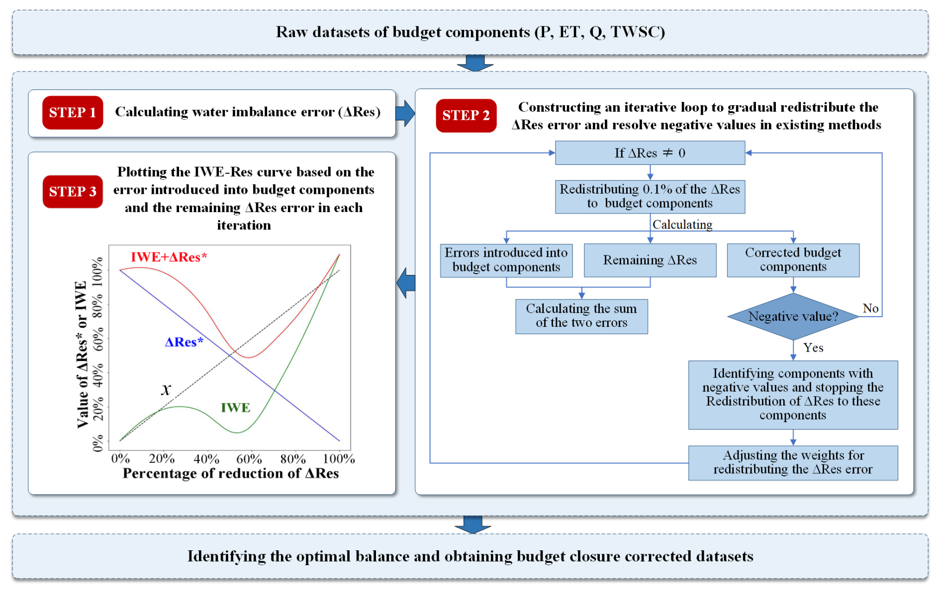
Figure 2 Framework of the IWE-Res method to identify the optimal balance for redistributing the ΔRes error. The x axis represents the proportion of ΔRes redistributed to budget components, while the y axis reflects the proportion of the remaining ΔRes error. The black dashed line represents the redistributed x-error value among the budget components. The blue solid line represents the ΔRes* curve, while the green solid line shows the IWE error introduced into budget components after redistributing the corresponding percentage of ΔRes. The red solid line represents the total error curve.

4 Results

4.1 Water imbalance error

This section presents a comparative analysis of variations in water imbalance errors across different basins and data combinations, aiming to clarify how errors in budget components contribute to these discrepancies. Figure 3 illustrates the spatial distribution of monthly ΔRes errors across various data combinations. To prevent the cancellation of positive and negative values, the absolute values of monthly ΔRes errors were first computed for each basin and then averaged.

As shown in Fig. 3, ΔRes values vary significantly across basins. Most basins in Africa, South America, and Europe exhibit high ΔRes values, typically exceeding 20 mm. In North America, ΔRes values generally range from 15 to 45 mm. Due to inconsistencies among budget component datasets, substantial differences in ΔRes also emerge across different data combinations. In combinations where only P data varied while other budget component datasets remained constant (combinations in Fig. 3 where the first digit varies while the second and third remain constant), pronounced changes in water imbalance errors were observed in parts of southern Africa, northern Asia, and North America. This suggests substantial estimation errors in P for these regions.

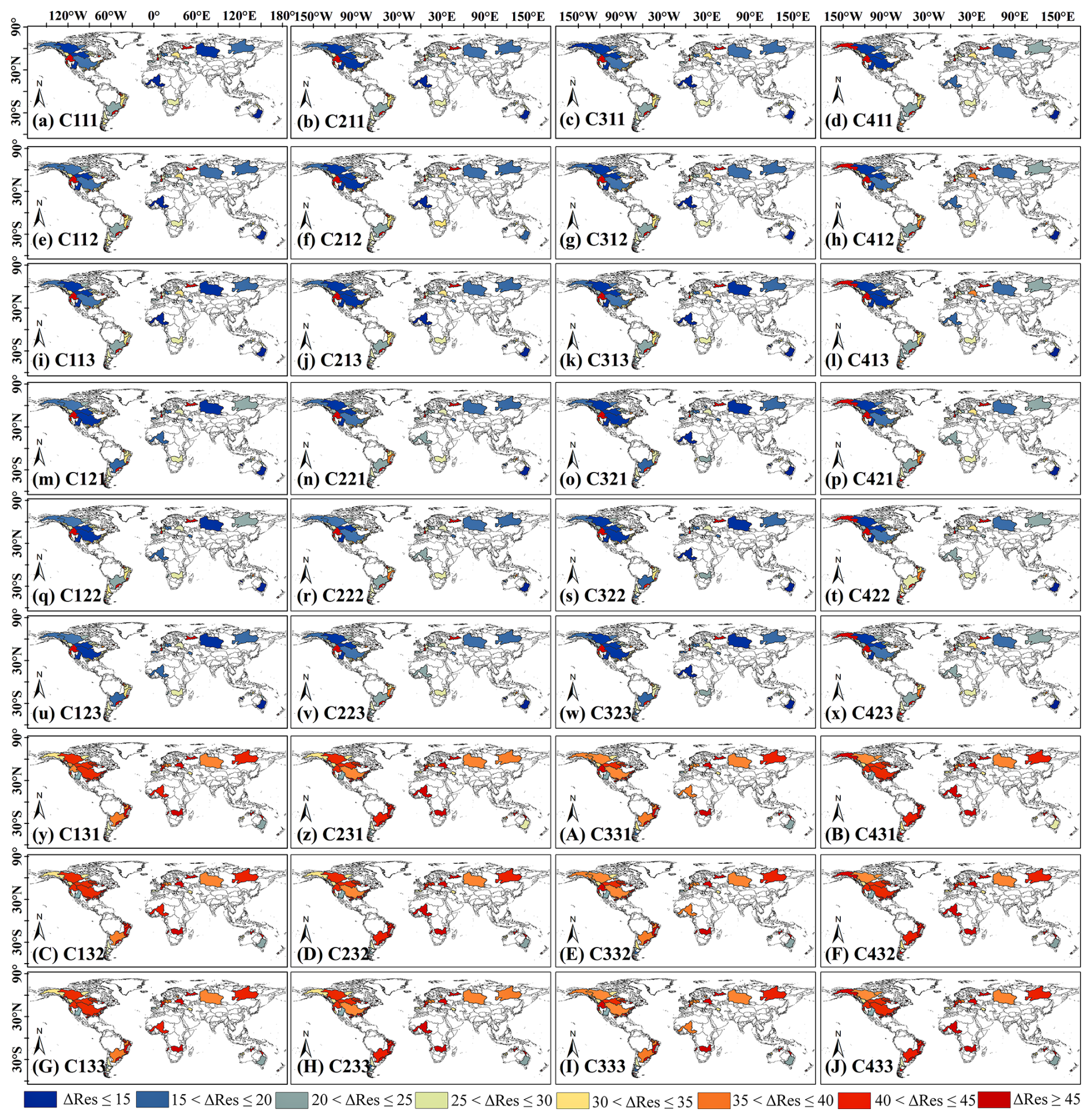
Figure 3 Spatial distribution of the ΔRes error on a monthly scale for different combinations of budget components. The unit of ΔRes is mm. Each subplot represents a distinct combination, where the first digit corresponds to the P product, the second to the ET product, and the third to the TWSC product. The detailed definitions of these combinations are provided in Eq. (3).

When different ET products were used (combinations where the second digit varies while the first and third remain constant), water imbalance errors changed significantly in most basins. Specifically, in combinations using the TerraClimate ET dataset, water imbalance errors exceeded 35 mm in the majority of basins, indicating severe water imbalance. This underscores the considerable discrepancies among ET products and their substantial impact on accurately representing basin water balance. In contrast, when TWSC data from different GRACE products were used (combinations where the third digit varies while the first and second remain constant), variations in water imbalance errors across basins were relatively small.

Overall, ET and P are the primary variables influencing water imbalance in most basins, consistent with previous findings (Pan et al., 2012; Zhang et al., 2018). The uncertainty in budget component datasets remains a key challenge for water balance research (Dagan et al., 2019; Lv et al., 2017; Luo et al., 2023a).

4.2 Uncertainties of budget components introduced by closing water budget

To gain a more comprehensive understanding of the uncertainties introduced into budget components when closing the water budget, this section analyzes the errors introduced by fully closing the water budget using existing BCC methods from three perspectives: the errors of individual budget components, the occurrence of negative values, and ensemble errors (Sect. 3.3).

4.2.1 Errors of individual budget components

Figure 4 presents the relative statistical metrics calculated using Eqs. (19)–(22) to evaluate the uncertainties introduced into budget components by existing BCC methods. Positive values indicate an improvement in the accuracy of corrected budget components, whereas negative values indicate a decline in accuracy.

Overall, existing BCC methods exhibit notable limitations in enhancing the accuracy of budget components. In particular, for P, nearly all statistical metrics (CC^′, NSE^′, MAE^′, RMSE^′) across various basins yield negative values. For instance, under the CKF method, these values are approximately −0.05, −0.15, −3.82, and −8.47 mm, respectively, indicating a significant reduction in the accuracy of the corrected P dataset when BCC methods are applied to enforce water budget closure. Specifically, the accuracy of the corrected P dataset decreases by approximately 6 %, 34 %, 11 %, and 55 %, as reflected in the CC, NSE, MAE, and RMSE metrics, respectively. Analysis of 13 selected basins with sufficient P observations further confirms this decline, showing a reduction in the accuracy of budget-corrected P (Fig. 5). A possible explanation for this decrease is the inherently high accuracy of raw P datasets, supported by advancements in remote sensing technologies, meteorological models, and observational networks. However, when BCC methods are applied, water imbalance errors from other budget components, such as ET, may be inappropriately redistributed to the corrected P dataset in an effort to enforce overall water budget closure. As a result, while the total water budget is balanced, the accuracy of the corrected P data is compromised.

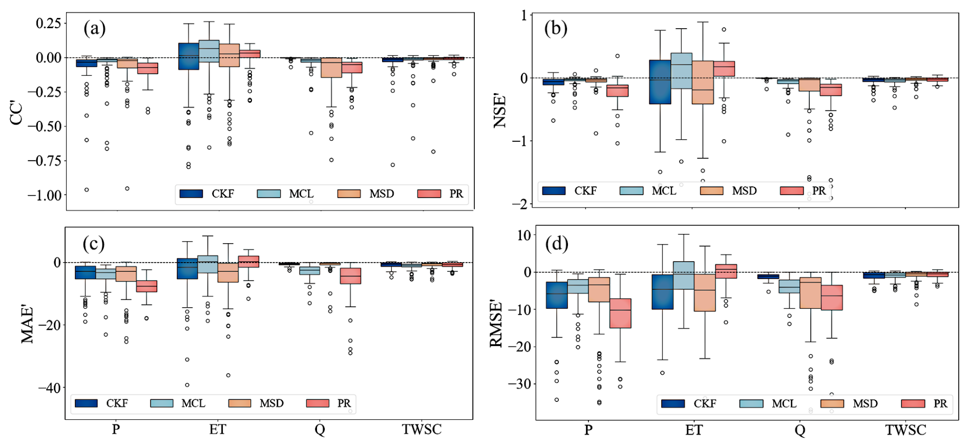
Figure 4 Box plot quantifying the errors introduced into budget components by existing BCC methods when closing the water budget. (a)–(d) represent the results of the CC^′, NSE^′, MAE^′, RMSE^′ indicators, respectively. Positive values indicate an improvement in accuracy relative to the reference values after applying existing BCC methods, while negative values indicate a decline. Different colors represent different BCC methods.

The impact of enforcing water budget closure using existing BCC methods on ET was particularly significant (Fig. 4), with approximately 50 % of basins exhibiting improved accuracy in corrected ET. For TWSC, most basins showed decreased accuracy. For Q, CC^′ and NSE^′ values ranged from 0 to −0.5, while MAE^′ and RMSE^′ were primarily concentrated between 0 and −20 mm. Consequently, the accuracy of corrected Q declined, with CC, NSE, MAE, and RMSE decreasing by approximately 0.1, 0.2, 3, and 5 mm, respectively. These findings indicate that while redistributing the entire ΔRes enhances the consistency of budget components, it provides limited improvement in their accuracy and may even introduce further errors. Identifying an optimal redistribution strategy for ΔRes errors could help mitigate this issue.

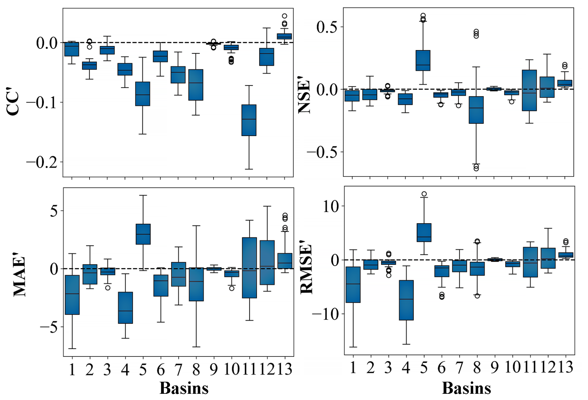
Figure 5 Box plot illustrating precipitation errors introduced by correcting ΔRes using existing BCC methods across 13 basins with sufficient observational precipitation data. The x axis represents the 13 basins in the following order: NIGER, OB, MISSISSIPPI, SACRAMENTO, SAN JOAQUIN, SUSQUEHANNA, BRAZOS, FRASER, NELSON, MURRAY, RIO EBRO, ELBE, and KURA.

4.2.2 Negative values

This section examines the occurrence of negative values in budget components arising from the application of existing BCC methods to close the water budget. For each budget component, the proportion of months with negative values relative to the total time series was computed (Fig. 6). Overall, the fraction of negative values across budget components ranges from 0 % to 10 %, with the majority falling below 5 %. This proportion is notable, as negative values indicate substantial inaccuracies in the redistribution of water imbalance errors by existing BCC methods. When a budget component exhibits a negative value, the accuracy of the remaining budget components is also compromised. The relatively high occurrence of negative values highlights the need for methodological improvements to enhance the performance of existing BCC methods.

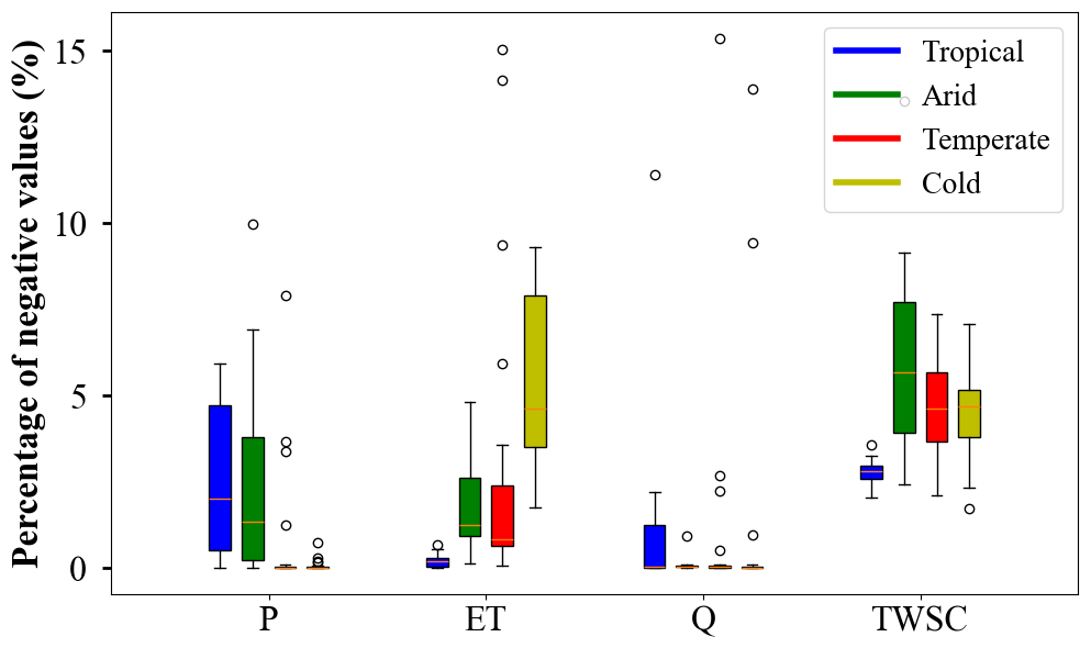
Figure 6 Percentage of negative values for corrected datasets of budget components induced by closing the water budget. Different colors indicate distinct climate classifications.

Among the individual budget components, ET and TWSC exhibit the most pronounced negative values, followed by P, while Q shows the least (Fig. 6). Notably, the proportion of negative values in budget components varies significantly across climate types. For P, negative values generally remain below 5 % but can occasionally reach 7 % in arid regions. The likelihood of negative P values is higher in tropical and arid climates (mostly below 5 %) compared with temperate and cold regions (around 1 %). For ET, the proportion of negative values is largely below 5 %, but it is notably higher in cold climates (reaching 9 %), followed by arid and temperate regions (approximately 1 %–3 %). Tropical climates exhibit the lowest proportion of negative ET values, with most instances below 1 %. Q consistently shows a low occurrence of negative values across all climate types (generally below 3 %), with a slightly higher probability in tropical regions than in other zones. The proportion of negative TWSC values ranges from 3 % to 10 %, being lowest in tropical climates (below 5 %), while other climate types exhibit values between 3 % and 10 %. Previous studies based on the Budyko framework (ignoring TWSC) at the annual scale have shown that water balance is primarily governed by P and potential ET (Sankarasubramanian and Vogel, 2002; Zhang et al., 2008; Koster and Suarez, 1999). However, these influences vary across climatic regions. For example, in tropical and arid regions, P tends to be the dominant controlling factor (Du et al., 2024; Wu et al., 2018; Liu et al., 2017; Guo et al., 2022). In cold regions, the Budyko model exhibits relatively limited accuracy in estimating ET at the annual scale (Lute et al., 2014; Gao et al., 2010; Potter et al., 2005). These previous findings at the annual scale provide indirect support for our results derived at the monthly scale.

Figure 7 presents the seasonal cycle of negative values across different climate zones, examining whether these values exhibit significant seasonal patterns. Negative P values predominantly occur in winter and spring, with a higher proportion from January to March in tropical climates compared to arid regions. ET tends to show negative values more frequently in winter and spring, with a lower likelihood in summer and autumn. Except in summer, cold climate zones are most susceptible to negative ET values. Among the four budget components, Q has the lowest occurrence of negative values. Negative TWSC values exhibit no obvious seasonal pattern, with arid regions exhibiting a higher likelihood of negative values throughout the year compared to other climate types. These findings indicate that the occurrence of negative values varies significantly across seasons and climate zones. Future research should account for this seasonal variability to further refine existing BCC methods.

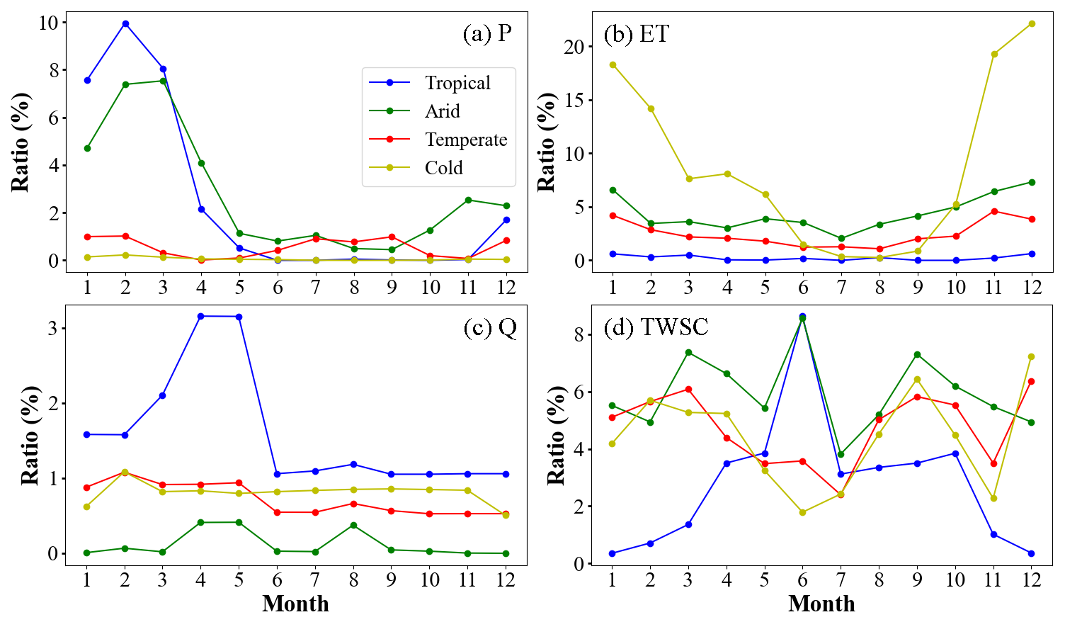
Figure 7 Seasonal cycle of the proportion of negative errors for budget components. Different colors representing various climate types. The Southern Hemisphere data by applying a 6-month shift to align its seasonal phases with those of the Northern Hemisphere.

4.2.3 Ensemble errors

Figure 8 presents the ensemble errors in budget components (i.e., F(Re) in Eq. 27) introduced by existing BCC methods (CKF, MCL, MSD, and PR). All four methods exhibit similar spatial distribution patterns. Notably, high ensemble errors (F(Re) >10 %) are concentrated in the northwestern basins of North America, particularly in Alaska, suggesting substantial variations in budget components in these regions. Basins with minor ensemble errors (5 % <F(Re) ≤10 %) generally cover larger areas, such as African and Northern Asia. Although these errors are relatively small, they remain non-negligible. Basins with lower ensemble errors (F(Re) ≤5 %) also cover some basins. Further analysis of ΔRes in basins with higher F(Re) values reveals a strong correlation, as these basins also exhibit larger ΔRes. This finding highlights the limitations of existing BCC methods in effectively redistributing ΔRes errors.

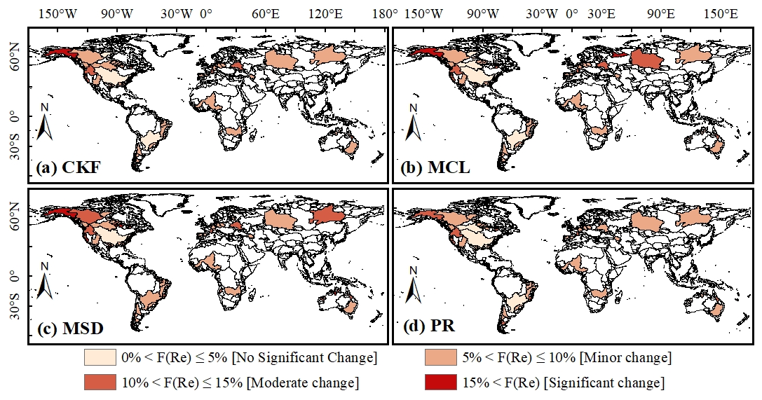
Figure 8 Ensemble errors in budget components introduced by closing the water budget using existing BCC methods.

To determine whether the error cost introduced by existing BCC methods in closing the water budget outweighs the reduction in water imbalance error, we analyzed the relationship between the reduction in ΔRes error and the introduced budget component errors (Fig. 9). As shown in Fig. 9, with the exception of the PR method, the basins where |RAE| exceeds |Res| are largely consistent across the other three BCC methods. This discrepancy arises because the PR method redistributes ΔRes based on the magnitude of budget components, whereas the CKF, MCL, and MSD methods redistribute ΔRes according to the estimated errors in budget components.

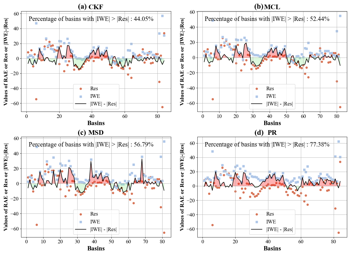
Figure 9 Comparison of relative absolute error (RAE) and residual error (Res) for four BCC methods (CKF, MCL, MSD, PR) across various basins. The black lines in the red shaded area on the upper half of the y axis indicate that the error introduced by the BCC methods for budget components exceeds the reduction in ΔRes error (|RAE$|>|$Res|), while the green shaded area on the lower half of the y axis represents cases where the error introduced is less than the reduction in ΔRes error (|RAE$|<|$Res|).

For the CKF, MCL, MSD, and PR methods, the proportions of basins where |RAE| exceeds |Res| are 44.05 %, 52.44 %, 56.79 %, and 77.38 %, respectively. This indicates that, for all four methods, the introduced |RAE| error in budget components surpasses the reduction in water imbalance error in more than 40 % of the basins. These findings underscore the non-negligible uncertainties introduced by these methods. Striking a balance between reducing water imbalance error and minimizing the impact of budget component errors remains a critical challenge, motivating us to propose the IWE-Res method to identify optimal balance.

4.3 Verifying the accuracy of the proposed IWE-Res method

Based on the error analysis of existing BCC methods in Sect. 4.2, this section assesses the accuracy and reliability of the proposed IWE-Res method. The evaluation is conducted through a comparative analysis with PR, CKF, MCL, and MSD, focusing on three key aspects: the errors of individual budget components, the occurrence of negative values, and ensemble errors.

Figure 10 compares the accuracy of the proposed IWE-Res method with existing PR, CKF, MCL, and MSD methods from the perspective of errors in individual budget components. The red and blue lines represent the IWE-Res method and the existing BCC methods, respectively, while the bars indicate the relative accuracy improvement of the IWE-Res method compared to the BCC methods. As shown in Fig. 10, the proposed IWE-Res method exhibits consistently higher accuracy than all existing CKF, MCL, MSD, and PR methods for budget components P, ET, Q, and TWSC. This result highlights the superior capability of the IWE-Res method in optimizing errors in budget corrected datasets. According to the statistical metrics CC, NSE, MAE, and RMSE, the proposed IWE-Res method improves the corrected P data by 4.2 %, 21.3 %, 25.5 % and 29.5 %, respectively, compared to the existing BCC methods. For corrected ET, the improvements are 6.9 %, 265.7 %, 17.6 % and 24.7 %, respectively; for corrected Q, the improvements are 3.4 %, 185.1 %, 67.1 %, and 69.0 %; and for corrected TWSC, the improvements are 0.0 %, 7.0 %, 7.5 %, and 6.8 %.

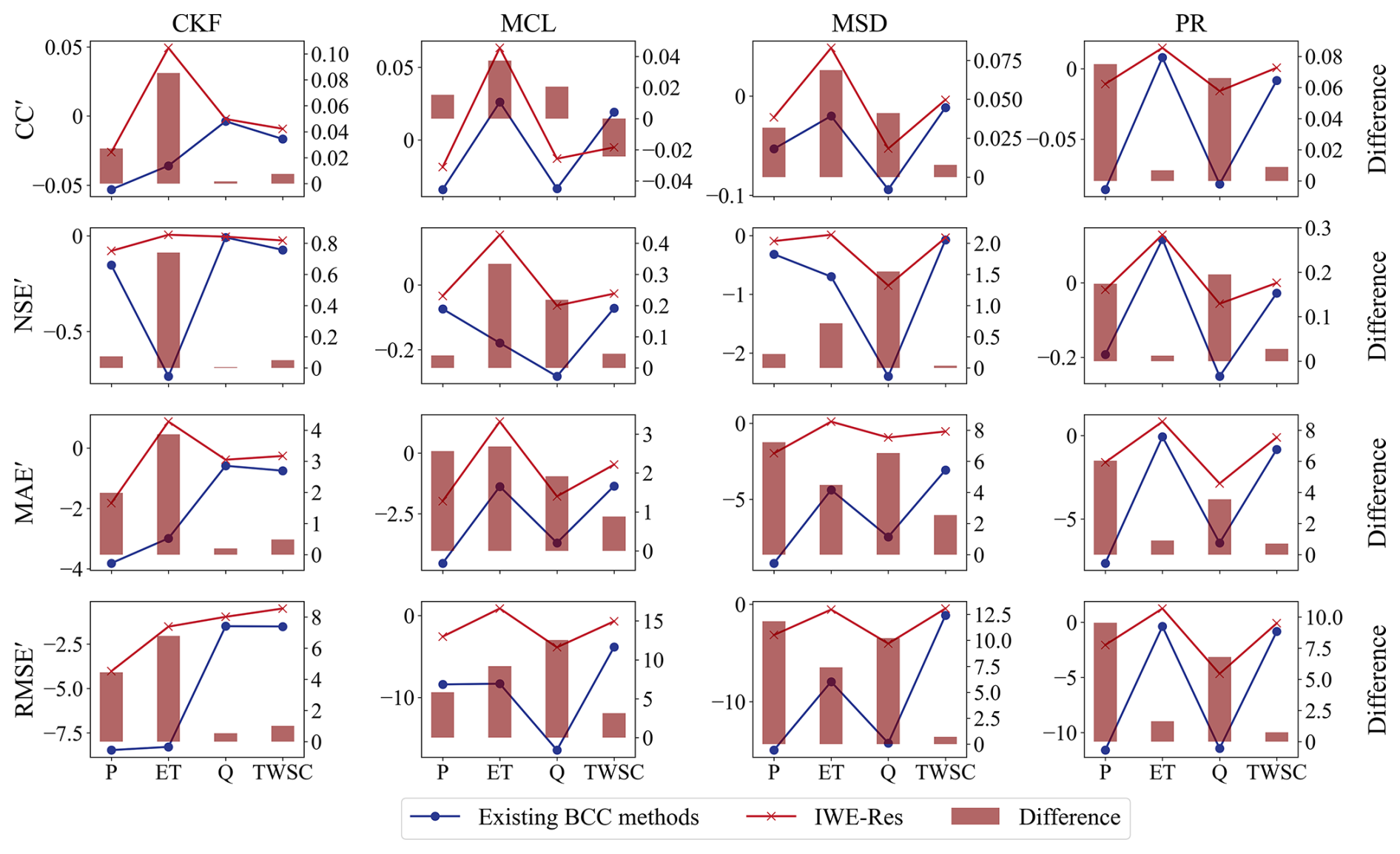
Figure 10 Performance comparison of the proposed IWE-Res method with existing BCC methods in corrected individual budget components. The red and blue lines in the figure represent the average values across all basins considered in this study.

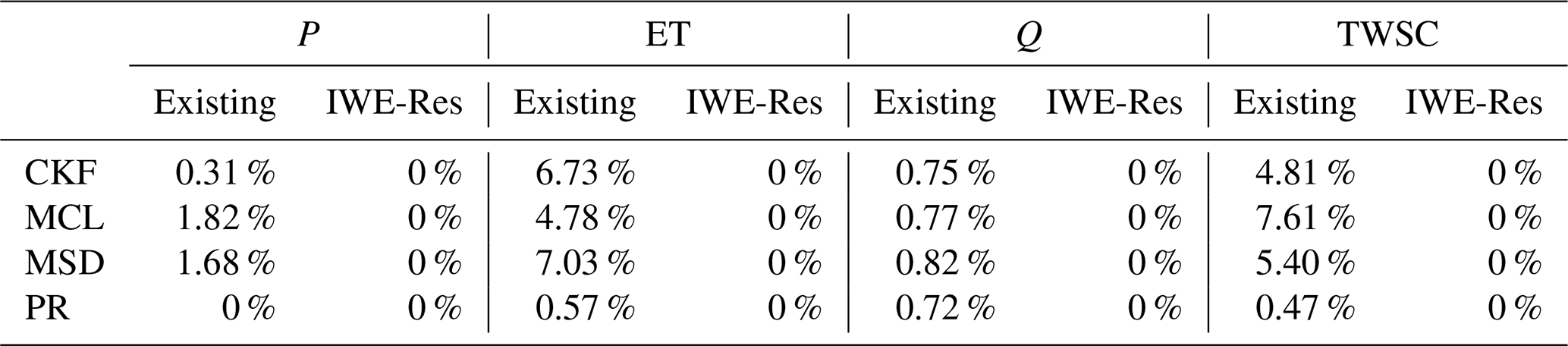
Table 2 presents the percentage of negative values observed in the corrected budget components for the proposed IWE-Res method and existing BCC methods. One of the key contributions of the IWE-Res method is its ability to address the critical limitation of negative value generation in existing BCC methods. As a result, the percentage of negative values in the corrected P, ET, Q, and TWSC data using the proposed IWE-Res method is zero. In contrast, the corrected P, ET, Q, and TWSC data obtained from existing BCC methods contain negative values to varying degrees (for a detailed analysis of negative values, see Sect. 4.2.2). These results demonstrate that, in addition to improving the accuracy of budget components relative to observations, the proposed IWE-Res method effectively eliminates the issue of negative values inherent in existing BCC methods.

Table 2 The percentage of months with negative values in the corrected datasets of budget components P, ET, Q, and TWSC for the proposed IWE-Res method and existing BCC methods. The percentages in the table represent the average values across all basins considered in this study.

We further evaluate the accuracy and reliability of the proposed IWE-Res method using the ensemble error metric defined by Eq. (27) (Fig. 11), where lower values indicate better model performance. As shown in Fig. 11, the IWE-Res method significantly reduces ensemble errors compared to existing BCC methods. For instance, in the CKF method, the median ensemble error decreases from above 5 % to below 5 %. This reduction is even more pronounced in the MCL, MSD, and PR methods. Additionally, the interquartile ranges under IWE-Res are notably narrower, suggesting improved control over stochastic variability. For example, in the PR method, the interquartile range shrinks from 5 %–8 % (existing BCC methods) to 1 %–2 % (IWE-Res), reflecting an approximate 67 % reduction in variability. These findings highlight the robustness of the IWE-Res method in minimizing integrated errors, aligning with its previously demonstrated excellence in single-variable error optimization and negative value elimination.

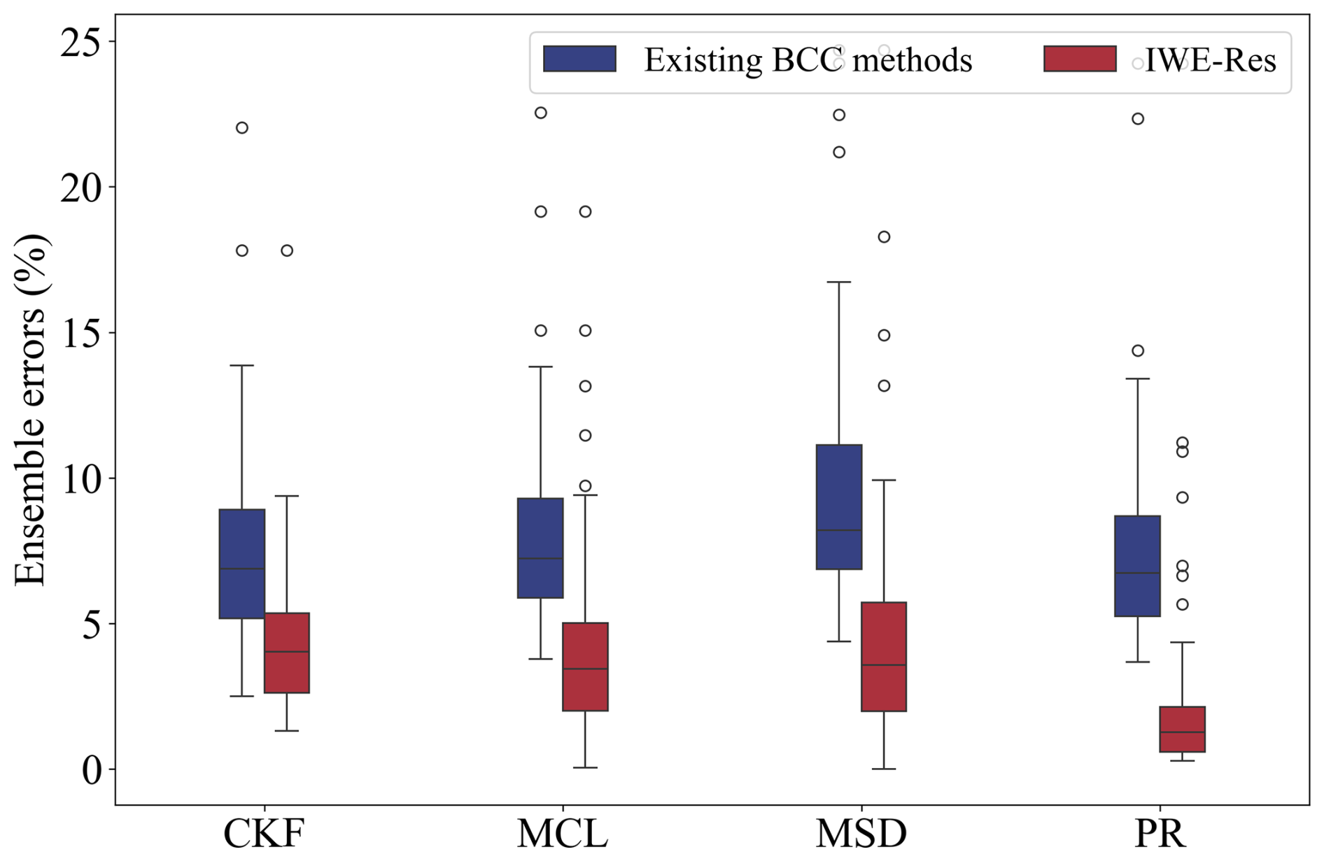
Figure 11 Performance comparison of the proposed IWE-Res method and existing BCC methods based on the ensemble errors of budget components.

4.4 Identifying the optimal balance for redistributing water imbalance error

Based on the proposed IWE-Res method, this section aims to determine the optimal balance for redistributing water imbalance errors across different climate zones (Tropical, Arid, Temperate, and Cold climate zones) to achieve the best trade-off (Figs. 12–15). Specifically, it seeks to minimize both water imbalance errors and the uncertainties in budget components introduced by enforcing water budget closure. The findings offer a valuable reference for generating high-precision datasets of budget components with a closed water budget in diverse climate regions. When developing the IWE-Res method, we incorporated multiple BCC methods, each based on different principles. As a result, the identified optimal balance results vary across methods. This section presents results for the CKF method only.

Overall, the optimal balance varied among basins located in different climate zones (Figs. 12–15). In most basins within the Tropical, Arid, and Temperate zones, the optimal balance was achieved when only a portion of the water imbalance error, rather than the entire error, was redistributed to budget components. However, this pattern was not observed in the Cold region.

For most basins in the Tropical climate zone (Fig. 12), the optimal balance was reached when 40 %–90 % of ΔRes was reallocated to budget components, suggesting that the corrected budget datasets achieve their highest accuracy within this range. Notably, approximately 20 % of basins attained their optimal balance when 80 %–90 % of ΔRes was redistributed, while about 70 % did so within the 40 %–50 % range. Therefore, in Tropical basins, if sufficient observational data are unavailable to precisely determine the optimal balance, redistributing 40 %–50 % of ΔRes to budget components is recommended to obtain the most accurate dataset.

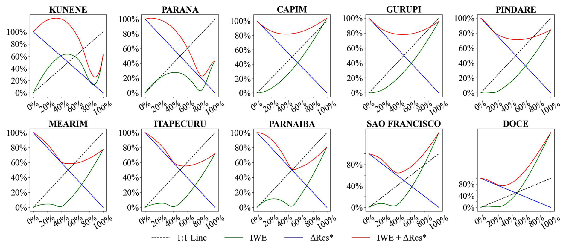
Figure 12 IWE-Res curve in basins of Tropical climate zone for identifying the optimal balance that enhances water budget closure and reduces uncertainty.

For basins in the Arid climate zone (Fig. 13), optimal balance are generally found when 40 %–90 % of ΔRes is redistributed, indicating that the corrected budget component datasets achieve their highest accuracy within this range. Specifically, approximately 31 % of basins reach their optimal balance at 40 %–50 % redistribution, 38 % at 60 %–80 %, and over 20 % at 90 %. Thus, the distribution of optimal balance in Arid basins does not follow a distinct pattern.

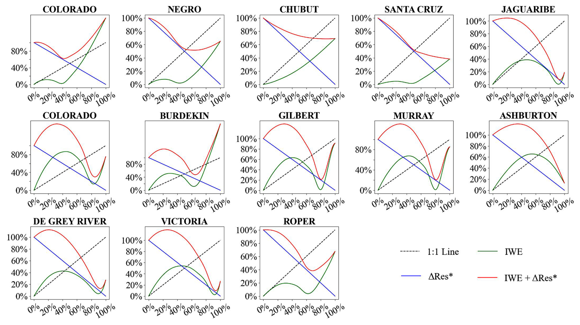
Figure 13 IWE-Res curve in watersheds of Arid climate zone for identifying the optimal balance that enhances water budget closure and reduces uncertainty.

In the Temperate climate zone (Fig. 14), optimal balance are concentrated within the 40 %–90 % range. Approximately 53 % of basins achieve their optimal balance when 40 %–50 % of ΔRes is redistributed, while 17 % and 13 % reach it at 70 % and 90 % of the ΔRes redistribution. A smaller proportion of basins achieve optimal balance at 60 % and 80 % of the ΔRes redistribution. Overall, redistributing 40 %–50 % of ΔRes minimizes the combined error from both the introduced budget component error and the remaining water imbalance error in most basins.

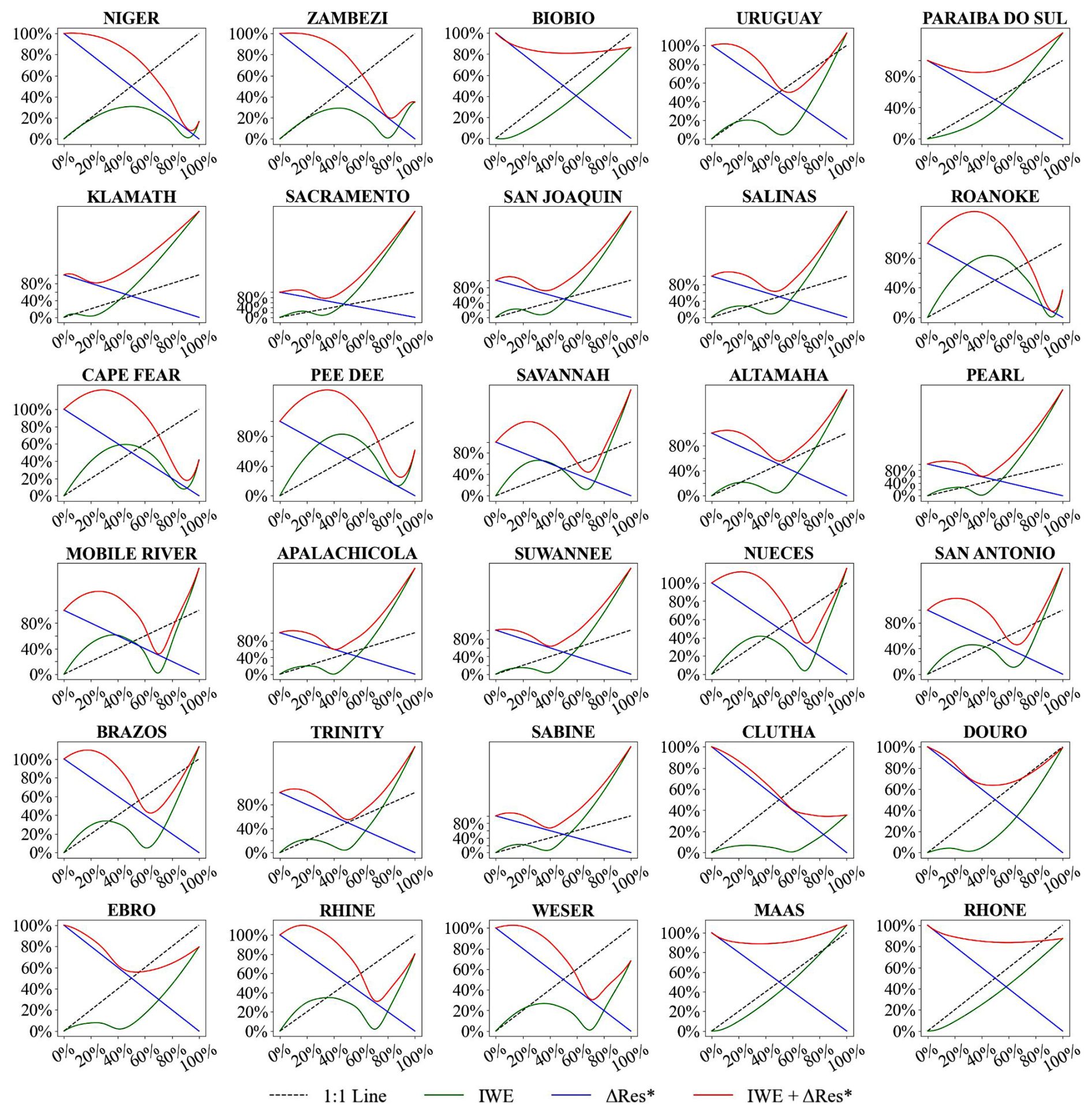
Figure 14 IWE-Res curve in watersheds of Temperate climate zone for identifying the optimal balance that enhances water budget closure and reduces uncertainty.

In Cold climate zone basins (Fig. 15), the optimal balance is typically reached when the entire ΔRes is fully redistributed. This suggests that complete redistribution of ΔRes does not compromise the accuracy of the budget components. This is primarily due to the trend observed in the IWE curve, which initially increases – indicating rising error – before decreasing, in contrast to the patterns seen in most basins in Figs. 12–14. A comparison of ΔRes and the negative values introduced by full redistribution of ΔRes across climate zones reveals that, in Cold regions, negative values predominantly occur in ET. This is likely due to the inherently lower ET values in Cold regions, which increases the likelihood of negative values when ΔRes is redistributed. However, errors introduced in other budget components, such as P and Q, remain relatively low under full redistribution of ΔRes.

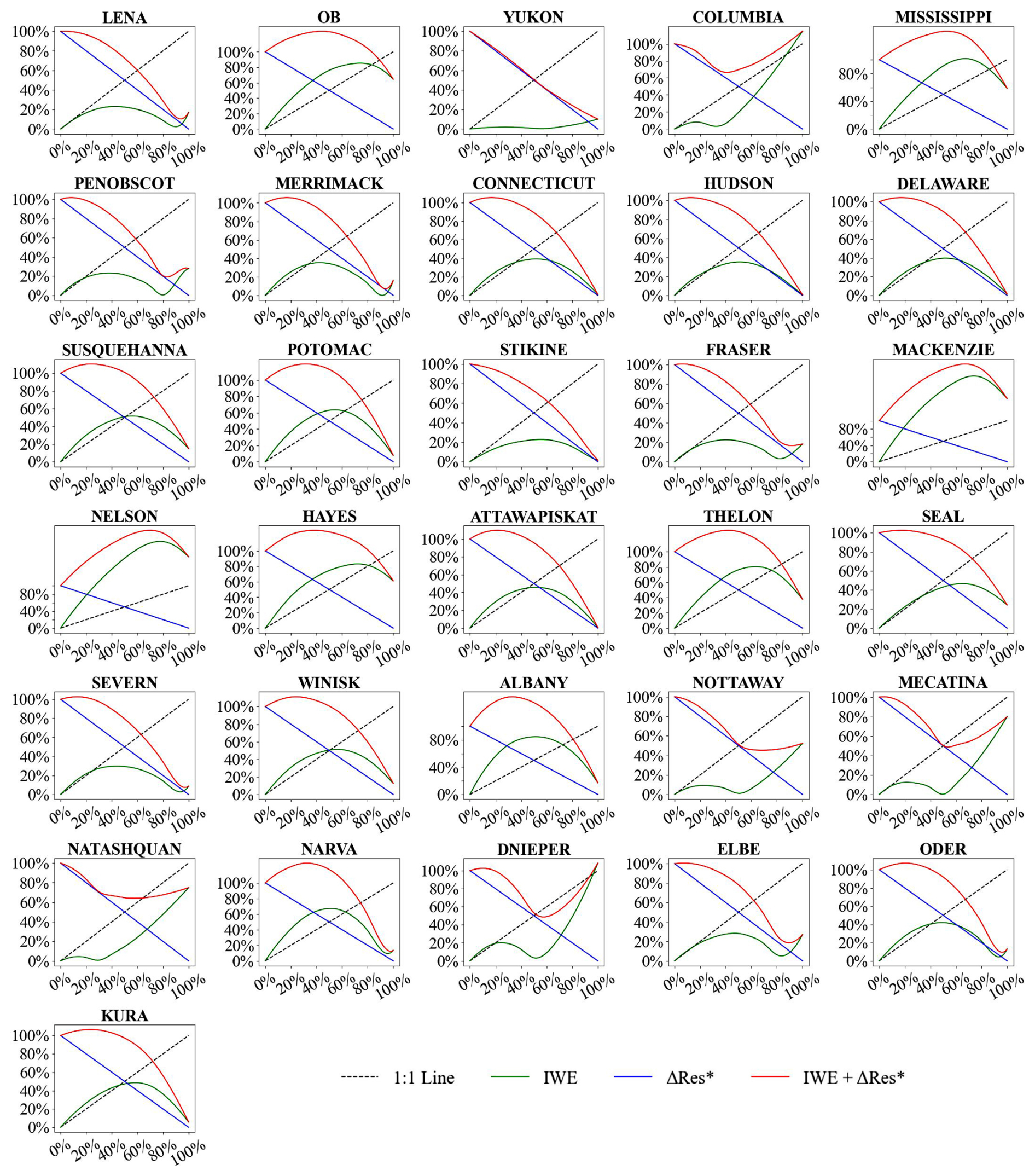
Figure 15 IWE-Res curve in watersheds of Cold climate zone for identifying the optimal balance that enhances water budget closure and reduces uncertainty.

5 Discussion

5.1 Uncertainty introduced by existing BCC methods

To quantify the uncertainty introduced by existing BCC methods in closing the water balance, we evaluated four BCC methods across 84 global basins. The assessment focused on errors in individual budget components, occurrences of negative values, and ensemble errors in budget components. Our findings indicate that while existing BCC methods improve the consistency of budget components, their ability to enhance the accuracy of these components is limited and, in some cases, may even reduce it. It is worth noting that the datasets generated by both the existing BCC methods and the IWE-Res method proposed in this study were not further bias-corrected against independent observations. For basin-specific applications requiring higher reliability, we recommend additional bias correction.

Several factors may contribute to this reduction in accuracy. First, most existing BCC methods estimate errors in budget components without incorporating independent observational data. These methods then redistribute water imbalance errors based on these internally estimated uncertainties (Sect. 3.2). However, the absence of observational constraints undermines the reliability of the estimated component errors, which in turn leads to a suboptimal and potentially biased allocation of the imbalance. As previously noted, inaccurate error estimates for a single variable can propagate through the redistribution process, biasing the residual redistribution to the remaining budget components and ultimately lowering the accuracy of all water budget components (Abolafia-Rosenzweig et al., 2021). Incorporating high-quality observational data into the error estimation process is therefore essential to improve the robustness of BCC methods; Second, existing BCC methods are limited by their assumption that the entire water imbalance error can be fully attributed to errors in the measured budget components. These methods enforce water budget closure by completely redistributing the water imbalance error among the budget components, yet this residual may also stem from systematic biases and unmeasured processes – not just estimation errors of measured budget components. In this study, we propose an iterative optimization approach that seeks a balanced redistribution of the ΔRes, aiming to minimize both the errors introduced to individual budget components and the remaining ΔRes. This method significantly improves the accuracy of the corrected datasets. Future research may further enhance this framework by integrating it with physically based hydrological or land surface models, which could provide a promising pathway toward more physically consistent and realistic water budget estimates; Third, the observational datasets themselves often fail to strictly satisfy water budget closure due to measurement limitations and sampling errors. This introduces uncertainty when using these datasets to validate the accuracy of BCC-corrected estimates. For instance, even if the corrected datasets more closely approximate the true values of budget components, the lack of ground-truth observations presents a fundamental challenge for objectively evaluating the effectiveness of these corrections. Future work should prioritize the development of more objective and physically grounded evaluation metrics to assess the accuracy of BCC-corrected datasets. Although this challenge lies beyond the scope of the present study, addressing it will be critical for advancing the reliability of water budget assessments.

5.2 Identification of the optimal balance

Each budget component inherently contains observational or model-based errors. Indiscriminately redistributing water imbalance errors across all budget components to achieve complete water budget closure can introduce additional uncertainties. By identifying the optimal balance for error redistribution across different climate zones, we observed significant variations in distribution patterns. In tropical and temperate regions, most basins achieved their optimal balance when 40 %–90 % of the water imbalance error was redistributed, with a concentration around the 40 %–50 % range. In arid regions, the distribution of optimal balance was more dispersed, lacking a clear concentration within any specific redistribution range but generally falling within the 40 %–90 % range. Cold climate regions exhibited distinct characteristics, with most basins achieving the smallest error when the water imbalance error was fully redistributed.

Overall, optimizing the redistribution ratio of water imbalance errors is critical for improving the accuracy of corrected budget components. However, the sensitivity of these components to error redistribution varies, and both over- and under-correction can propagate new imbalances across the remaining terms, ultimately misrepresenting the underlying hydrological processes. While existing BCC methods estimate redistribution weights based on the relative uncertainty of each component, future research should examine the physical rationale behind these redistributions. The spatiotemporal variability of residual errors offers valuable insight into their dominant sources, which can serve as an independent reference to validate the influence weights computed by BCC methods. For instance, as shown in previous studies, the contribution of TWSC to residual errors diminishes at annual and especially decadal timescales, where P and ET uncertainties become more dominant. Spatial patterns of residuals also reflect the nature of regional precipitation regimes. In regions dominated by frontal systems, such as temperate zones, remotely sensed precipitation products tend to capture rainfall events more accurately, leading to smaller residuals. In contrast, in areas characterized by convective rainfall – such as the tropics and arid zones – larger residuals are observed, likely due to the higher uncertainty in capturing short-lived and spatially localized storm events.

Notably, the choice of spatial resolution has a significant impact on the results (Aziz et al., 2022; Bormann, 2006; Senan et al., 2022). Following many previous studies (Lehmann et al., 2022; Abolafia-Rosenzweig et al., 2021; Luo et al., 2023c; Wang et al., 2014; Tan et al., 2022; Sahoo et al., 2011), the BCC method in this study is also applied at the basin scale rather than the grid scale for the following reasons: (1) Achieving water budget closure at the grid scale is complex and challenging due to the difficulty of quantifying all water flux and storage components flowing into and out of the grid, including P, ET, TWSC, lateral inflow and outflow, leakage losses, and human water withdrawals and returns. Several of these components, such as lateral flow and leakage, are poorly observed or highly uncertain, and their omission introduces substantial error; (2) The datasets of different variables have varying spatial resolutions, and resampling them to a common resolution introduces uncertainties, which in turn affect the accuracy of water budget closure correction; (3) The coarse spatial resolution of GRACE-derived TWSC data limits their applicability for water budget closure calculation at the grid scale. At monthly resolution, TWSC is a critical component and cannot be neglected. Averaging GRACE data to the basin scale helps reduce random errors by offsetting positive and negative biases, thereby increasing the reliability of water budget closure correction; (4) Despite advances in remote sensing and in situ observation networks, grid-scale uncertainties remain substantial for some budget components, such as ET. Basin-scale analysis therefore reduces uncertainty and improves the reliability of water budget closure correction results.

6 Conclusions

Existing BCC methods introduce new uncertainties when closing the water budget due to challenges in accurately estimating errors in budget components and the integrated concept of water imbalance error. This study first evaluates the issues arising from existing BCC methods by comparing the errors introduced in budget components with the improvement in water budget closure precision. A new method, termed IWE-Res, is proposed to identify the optimal redistribution of ΔRes, aiming to minimize the sum of the remaining residual error and the introduced budget component error. To assess the reliability of the IWE-Res method, we compare it with four different BCC methods across 84 basins spanning various global climate zones. The main conclusions are as follows:

1. While applying existing BCC methods reduces water imbalance error, it simultaneously introduces new errors in budget components. For P, a decline in accuracy is observed in most basins. For Q, the corrected data exhibits lower performance than the raw data, with reductions in CC, NSE, MAE, and RMSE of approximately 0.1, 0.2, 3, and 5 mm, respectively. At the basin scale, more than 40 % of basins experience budget component errors greater than the reduction in ΔRes after applying existing BCC methods.

2. The proportion of negative corrected values in each budget component is predominantly within 0 %–5 %. For ET, negative corrected values are mostly below 5 %, though they reach 9 % in cold climate regions. For P, the proportion is primarily below 5 %, with rare occurrences around 7 %. Q generally exhibits a lower proportion of negative values, mostly below 3 %. In TWSC, negative values are concentrated between 3 % and 10 %.

3. The proposed IWE-Res method improves the accuracy of corrected budget components compared to existing BCC methods. Based on RMSE, it improves the accuracy of corrected P by 29.5 %, corrected ET by 24.7 %, corrected Q by 69.0 %, and corrected TWSC by 6.8 %.

4. Except in cold regions, redistributing 40 %–90 % of ΔRes to budget components yields the optimal balance, minimizing the sum of the remaining ΔRes and the introduced budget component error. In tropical and temperate regions, the optimal balance is typically achieved when 40 %–50 % of ΔRes is redistributed. Similarly, in arid regions, redistributing 40 %–90 % of ΔRes effectively reduces errors, though the optimal redistribution ratio varies across basins. In most cold-region basins, the total error is minimized when the entire ΔRes is redistributed.