Assessing the adequacy of traditional hydrological models for climate change impact studies: a case for long short-term memory (LSTM) neural networks

Climate change impact studies are essential for understanding the effects of changing climate conditions on water resources. This paper assesses the effectiveness of long short-term memory (LSTM) neural networks compared to traditional hydrological models for these studies. Traditional hydrological models, which rely on simplified process parameterization with a limited number of parameters, are examined for their capability to accurately predict future hydrological streamflow under scenarios of significant warming. In contrast, LSTM models, known for their capacity to learn from extensive sequences of data and capture temporal dependencies, present a promising alternative. This study is performed on 148 catchments, comparing four traditional hydrological models, each calibrated specifically on each catchment, against two LSTM models. The first LSTM model is trained regionally across the 148 catchments, while the second incorporates data from an additional 1000 catchments at the continental scale, many located in climate zones representative of the future climate within the study domain. The climate sensitivity of all six hydrological models is assessed using four simple climate scenarios (+3, +6 °C, −20 %, and +20 % mean annual precipitation) and an ensemble of 22 CMIP6 GCMs under the SSP5-8.5 scenario. Results indicate that LSTM-based models demonstrate a different climate sensitivity compared to traditional hydrological models. Moreover, analyses of precipitation elasticity to streamflow and multiple streamflow simulations on analogue catchments suggest that the continental LSTM model performs better and is therefore better suited for climate change impact studies – a conclusion that is also supported by theoretical arguments.

1 Introduction

A warming climate has profound cascading impacts affecting the entire biosphere (e.g. Bellard et al., 2012; Jackson, 2021; Scheffers et al., 2016). The potential influence of an evolving climate is typically assessed through climate change impact studies. These studies evaluate the impacts of climate change on environmental, economic, and social systems. They cover how a changing climate affects ecosystems and the weather and how it ultimately impacts the human population and infrastructures. Impact studies are a critical tool to enable efficient adaptation strategies addressing climate-related challenges.

There are many different ways to conduct impact studies, but the most common approach is to use a top-down modelling chain connecting general circulation or Earth system models (GCM for short) to a specific impact model such as a crop (Jägermeyr et al., 2021), forest fire (Dupuy et al., 2020), or hydrological model (Hagemann et al., 2013; Minville et al., 2008). A climate change impact study should not only quantify future changes but also the uncertainty in the projected change (Chen et al., 2011; Clark et al., 2016; Wilby and Harris, 2006).

To adequately frame climate change impact uncertainty, the importance of incorporating multiple GCMs cannot be overstated. GCMs are instrumental in projecting future climate scenarios, yet the inherent uncertainty in their climate sensitivity – defined as the equilibrium climate sensitivity (ECS), which quantifies the Earth's temperature response to a doubling of carbon dioxide concentrations (CO₂) – presents a significant challenge. Given the variability in the ECS among different GCMs (Hausfather et al., 2022), leveraging a suite of GCMs is essential to adequately sample this pivotal source of uncertainty, thereby enhancing the robustness of climate projections. This has been the norm for many years, as reflected in a multitude of climate change impact studies in hydrology and other fields (e.g. Chen et al., 2012; Deb et al., 2018; Martel et al., 2022; Thompson et al., 2013; Wang et al., 2020).

The climate sensitivity of impact models has comparatively been much less studied but has nonetheless been shown to be significant (Brigode et al., 2013; Giuntoli et al., 2018; Kay et al., 2009; Krysanova et al., 2018; Mendoza et al., 2015; Poulin et al., 2011), sometimes to the point of being more important than that of GCMs (Her et al., 2019). The climate sensitivity of impact models is dependent on the parameterization of various (and often simplified) processes. The calibration parameter sets are typically optimized for historical climatic conditions (e.g. Althoff and Rodrigues, 2021; Chlumsky et al., 2021) and may not be well suited to future climates, especially under scenarios of significant warming. Recognizing and evaluating the uncertainty tied to impact model sensitivity is crucial and is typically approached by employing multiple impact models or multiple parameter sets when feasible. However, using multiple impact models without a priori knowledge of their transferability to a different climate is a likely path towards an overestimation of impact model uncertainty, which is as likely to lead to maladaptation as underestimating it (Sem, 2007). Mearns (2010) and many others emphasize the crucial importance of correctly framing uncertainty to help decision-makers adopt proper adaptation measures.

In hydrology, this has spurred a body of literature focused on refining models and calibration approaches for hydrology models to better account for future climate variability and change. Using physically based hydrological models (Feng et al., 2023; Michel et al., 2022) or best-performing models (Li et al., 2015) has been proposed as a more robust alternative. However, such models typically require complex observational inputs that are often not available, and even the most physical models do require some level of parameterization. Hydrological models always had to contend with internal climate variability, and this is why a calibration period should be as long as possible, as argued by Arsenault et al. (2018) and Shen et al. (2022) for optimal robustness. They suggest that by maximizing the length of the calibration time series, it exposes the models to more contrasted conditions and therefore improves robustness. However, internal climate variability over a typical calibration historical period remains small compared to end-of-century climate projections, especially for near-surface temperature. To address this, multi-model approaches (Arsenault et al., 2015; Seiller et al., 2015) and various split-sample procedures have been proposed to study model robustness over contrasting periods, such as dry/wet or cold/hot periods (e.g. Bérubé et al., 2022; Coron et al., 2012; Thirel et al., 2015; Vansteenkiste et al., 2014). Ultimately, none of the above approaches have proven particularly convincing. In particular, Bérubé et al. (2022) conducted a large-sample study of contrasting-condition calibration strategies and showed that no single calibration strategy or length was successful for all metrics and study catchments. Some of the underlying reasons for that are discussed by Duethmann et al. (2020), including issues with precipitation data – such as evolving measurement networks that alter statistical properties – and the neglect of changes in vegetation over time. Finally, the large number of studies on regionalization also demonstrated that hydrological models have a relatively limited transferability to other catchments even in similar climate zones (Arsenault and Brissette, 2014b; Guo et al., 2021; Parajka et al., 2013; Tarek et al., 2021).

In this context, deep-learning models may have the ability to overcome such problems (Althoff et al., 2021; Wi and Steinschneider, 2022; Zhong et al., 2023). In particular, long short-term memory (LSTM; Hochreiter and Schmidhuber, 1997) networks offer a promising alternative. LSTM models are a special kind of recurrent neural network (RNN) architecture which can learn from sequences of data by capturing temporal dependencies and relationships. They are specifically designed to avoid the long-term dependency problem of vanishing or exploding gradients during training. Their unique architecture enables them to learn and remember over longer sequences of data compared to RNNs, making them highly effective for predictions of time series. In addition, unlike traditional conceptual models that are typically calibrated on data from a single catchment or from a small number of catchments pooled together (Gaborit et al., 2015; Ricard et al., 2013), LSTM models are trained across a diverse array of catchments, encompassing a wide range of climatic conditions and physical characteristics, potentially covering a range similar to or beyond that expected due to climate change over many catchments. For these reasons, this methodological shift is anticipated to yield models with enhanced robustness to varying climate scenarios. Kratzert et al. (2019a, b) underscored this potential, demonstrating that a regional LSTM model can significantly outperform traditional hydrological model regionalization methods, which rely on locally calibrated models. This was then validated on independent datasets by Arsenault et al. (2023), Li et al. (2022) and Nogueira Filho et al. (2022). Kratzert et al. (2024) provided a rationale on why LSTM-based hydrological models should always use more than one catchment for training. Essentially, deep-learning approaches require a large amount of data to be trained properly, and including more data allows the model to better detect patterns and relationships between catchment descriptors, meteorological forcings, and the target streamflow.

The implementation of LSTM-based regional hydrological models is an alternative to traditional “trading space for time” methodologies. Trading space for time is an approach used in ecological and environmental studies to infer long-term environmental changes by examining spatial gradients at a single time point. In the context of climate change, this method assumes that spatial variations across different geographical regions can serve as proxies for temporal changes, thereby allowing researchers to predict the effects of climate change over time by observing current spatial patterns (Singh et al., 2014). Using LSTM models for hydrological simulation under changing climate conditions could likewise be compared to methods based on climatic analogues. Analogue-based methods, which identify past weather patterns similar to those projected for the future, offer an intuitive way to understand potential climate impacts by drawing direct parallels with historical events (e.g. Ford et al., 2010; Ramírez Villegas et al., 2011). While such methods provide valuable insights, particularly in elucidating the practical implications of climate projections, they inherently rely on the assumption that past climate variability is a sufficient proxy for future conditions. This assumption may not always hold, especially under scenarios of unprecedented climate change. However, by including a larger sample of catchments from varied climatic zones, LSTM models could have enough information to stay in interpolation mode, even at the upper end of future climate change estimates.

The objectives of this paper are threefold. The first is to assess the performance of an LSTM-based hydrological model in a climate change impact study, focusing on its potential ability to capture future hydrological streamflow. The second is to compare the future streamflow projections derived from the LSTM-based model against those obtained from conventional hydrological models, aiming to identify differences in the response across a spectrum of streamflow metrics and multiple catchments. Finally, the third objective is to explore the climate sensitivity of the LSTM-based model in contrast to traditional hydrological models, thereby contributing to a deeper understanding of LSTM-based hydrological model uncertainties in climate impact studies.

2 Study area and data

This section covers the study area, the data used to train the traditional and LSTM-based hydrological models, the various analyses to investigate the climate change impact on hydrological simulations, and the evaluation metrics used in this study.

2.1 Study area

This study focuses on a collection of 148 catchments located in the northeastern region of North America. These catchments are characterized by their exposure to snow-related processes, including accumulation and melt phases, playing a significant role in their hydrological dynamics. The selection of these catchments was done through the comprehensive HYSETS database (Arsenault et al., 2020, 2024a), which catalogues over 14 425 North American catchments, complete with hydrological, meteorological, and geophysical data. The choice of this specific subset was motivated by a previous study in which the same catchments were used in the context of predicting streamflow in ungauged basins (Arsenault et al., 2023). The LSTM models in that study proved to outperform conceptual hydrological models for this task, paving the way to the present study to determine how regional LSTM models can integrate spatially diverse information to predict streamflow in changing conditions. This is akin to a trading space for time approach using the LSTM model to do the work. This diversity is particularly pronounced between the southern and northern catchments, with notable differences in peak streamflow timings and precipitation rates, necessitating a detailed modelling approach beyond simple area-based extrapolations. In the Arsenault et al. (2023) study, only those catchments with a drainage area exceeding 500 km² were included, thereby sidestepping potential issues related to scale and time lag in model regionalization efforts. Catchments also required at least 30 years of data over the 1979–2018 period to be selected in order to have sufficient data to train both the conceptual hydrological models and the deep-learning implementations. The basin selection criterion was set to a minimum of 30 years of data to ensure not only a sufficient data length but also a robust sample of basins for performance assessment. This criterion was also used in this study, resulting in the selection of the same 148 catchments for the analysis.

For one LSTM configuration in this study, an extra set of 1000 donor catchments was added. This was done to determine if adding information from more catchments with different climate and physical characteristics could help increase the regionalization ability of the LSTM models and in turn help increase reliability in terms of climate change impact studies. This was performed by first widening the spatial extents of the study area and pre-selecting catchments with more than 20 years of available streamflow data within the new spatial bounds, as shown in Fig. 1a and b. Note that the 20-year limit differs from the 30-year limit used for the study catchment selection to widen the set of available catchments for this analysis, but these were not as critical as the original 148 as they were not used for model testing. Therefore, this constraint was relaxed to 20 years for the extra set of catchments. From there, 1000 donor catchments on top of the initial 148 were selected at random to be included in the extended LSTM model's training, with a larger distribution of these catchments being from more southern regions of the United States. This was done to ensure warmer catchments would be included in the training of the extended LSTM model, aiming to improve its ability to simulate a warmer climate in the northeastern North America catchments. The LSTM configuration trained on the study's 148 catchments will be referred to LSTM-R (regional), while the one trained using the additional 1000 donor catchments will be referred to LSTM-C (continental) throughout the paper.

2.2 Data

2.2.1 Meteorological and hydrometric data

All hydrological models in this study shared the same meteorological datasets to ensure a fair comparison between models and model types. Indeed, while conceptual models are limited in their type of meteorological inputs, deep-learning models can ingest any type of data and extract useful information if it is available. Therefore, the dataset that was the common denominator (i.e. the one that corresponds to the intersection between both datasets) for all models was used for all models. This consists of maximum and minimum daily temperature, as well as daily rainfall and snowfall. These data were initially provided through the ERA5 reanalysis dataset (Hersbach et al., 2020) but were directly used from the HYSETS database as they were already catchment-averaged and processed at the daily scale for all catchments in this study. Tarek et al. (2020) showed that daily ERA5 data can be used for hydrological modelling applications as a replacement for observed datasets with little to no loss in performance, while ensuring no missing data for the entire period. Meteorological data therefore covered the period 1980–2018 inclusively.

Hydrometric data were taken from the HYSETS database as well and covered the same period as the meteorological data. However, observed streamflow records contain many missing data, which justifies the use of catchments that only had at least 20 years of observed streamflow in the catchment selection (and 30 years for the 148 basins used for testing).

Boxplots will be used throughout this paper to outline study results (Wickham and Stryjewski, 2011). A boxplot is a concise graphical tool which highlights the central tendency (median), variability (interquartile range; IQR), and outliers (data extending beyond the whiskers or 1.5 times the IQR) within the distribution of results across all of the study catchments.

Figure 1 presents a first comparison between the meteorological data of the initial 148-catchment set (regional dataset – large circles in Fig. 1) and the 1000-catchment extension (continental dataset – small circles) using maps and boxplots. Specifically, the regional dataset encompasses a narrower climatic range, with mean annual temperatures varying from 0.5 to 11.1 °C and precipitation levels spanning 809 to 1425 mm. Conversely, the continental group dataset extends these boundaries significantly, covering a broader spectrum of climate conditions. This dataset records mean annual temperatures ranging from −9.1 to 21.8 °C and total precipitation ranging from 328 to 1570 mm.

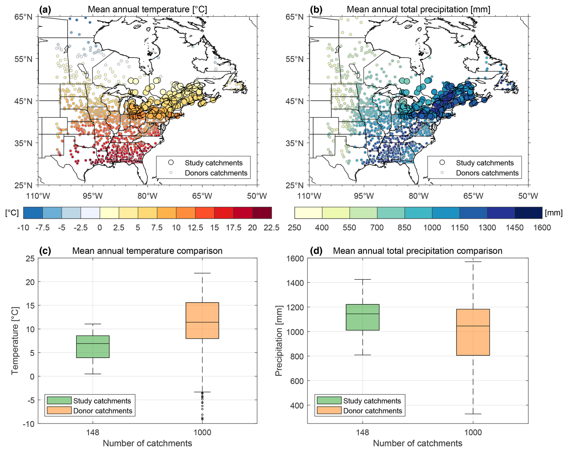
Figure 1 Maps (a, b) of study area showing the location of the 148 studied catchments (large circles with black outline) and the 1000 donor catchments for the continental LSTM model (small circles with grey outline). The fill colour represents the mean annual temperature (a) and total precipitation (b) of each catchment. The circles are located at the centroid of each catchment. Boxplots showing the comparison of mean annual temperature (c) and total precipitation (d) across the target sample of 148 catchments (green boxes) and the 1000 donor catchments (orange boxes) for the continental LSTM simulation.

Such a wide range of key climatic variables enables a comprehensive assessment of climate impacts across a wider geographic area. The extended range of the continental dataset is particularly critical for the development of robust LSTM models. By incorporating a broader spectrum of mean annual temperatures and precipitation, the continental dataset not only captures significant variability within climate data but also enhances the model's capacity to generalize across a diverse array of climate conditions. This aspect is especially beneficial for anticipating and adapting to a future warmer climate, where the variability and extremities of climate conditions are expected to intensify.

2.2.2 Catchment descriptors

Catchment descriptors are required for regional LSTM-based hydrological modelling, as the simulated streamflow is a function of not only the meteorological data, but also the catchment properties. These descriptors allow the LSTM models to learn patterns and relationships to modulate and adjust simulated streamflow based on each catchment's static properties. This has already been implemented in Kratzert et al. (2019a) and Arsenault et al. (2023). The catchment descriptors used in this study represent geographic (i.e. catchment's drainage area, elevation, slope, aspect, perimeter, and Gravelius index), land-use (i.e. fraction of crops, forests, grass, shrubs, water, wetlands, and urban areas), and geologic (i.e. permeability and soil porosity) descriptors, for a total of 15 descriptors. These are a subset of those used successfully in Arsenault et al. (2023) and are presented in Fig. S1.

2.3 Hydrological models

2.3.1 Traditional hydrological model setup

The traditional hydrological models are characterized by their lumped and conceptual nature, enabling local calibration across the large array of catchments used in this study. Meteorological data from all ERA5 grid points within the drainage area boundary of each catchment were averaged due to the lumped structure of the models. A total of four traditional hydrological models with a relatively wide range of potential evapotranspiration (PET) estimation methods and degree-day snow models were used as a benchmark for comparison with the LSTM-based models.

1. GR4J (French for Model of Rural Engineering with four parameters – Daily) is a parsimonious four-parameter lumped model developed by Perrin et al. (2003). Due to its limitation in simulating snow processes, it has been coupled with a two-parameter variant of the simple degree-day snow model CemaNeige proposed by (Valéry et al., 2014), thereby ensuring a basic representation of the evolution of the snow cover. This integration results in a hydrological model termed GR4J_CN, which comprises a total of six parameters. PET was computed using the Oudin formula (Oudin et al., 2005), which is a variant from the McGuinness and Bordne (1972) that showed the best performance among 27 other PET formulas for the simulation of streamflow. Previous studies have demonstrated the effectiveness of this model structure in accurately simulating continuous daily streamflow for snowmelt-dominated catchments similar to those used in the regional dataset of this study (Troin et al., 2015, 2018; Dallaire et al., 2021).

2. HMETS (Hydrological Model – École de technologie supérieure; Martel et al., 2017), a 21-parameter lumped hydrological model, stands as a simple model originally designed for research and educational purposes. One notable feature of this model is its snow model based on the work of Vehviläinen (1992), a 10-parameter degree-day model which enables the representation of the snowpack's melting and refreezing process. The relatively large number of parameters allows it to provide good performance on a wide variety of catchments across North America as shown by Martel et al. (2017). Similar to GR4J_CN, PET was provided to the model by the Oudin formula (Oudin et al., 2005).

3. HSAMI, a 23-parameter lumped model, has been utilized for daily streamflow forecasting across over 100 catchments by Hydro-Québec, a prominent hydropower producer. A simple empirical PET formula based on minimum and maximum temperature is used by HSAMI:

   $$\begin{array}{}\text{(1)}& \begin{array}{rl}\mathrm{PET}& =\mathrm{0.0029718}\cdot (T_{\max }-T_{\min })\\ & \cdot e^{(\mathrm{0.0342}\cdot \left(T_{\max }+T_{\min }\right)+\mathrm{1.216})},\end{array}\end{array}$$

   where temperatures are in degree Celsius (°C) and PET in centimetres per day (cm d⁻¹). The model uses a six-parameter degree-day snow model, allowing us to simulate the processes linked with accumulation of snow, rain interception, and melting of the snow cover. HSAMI has found application in various hydrological and climate change impact studies, such as those conducted by Minville et al. (2008), Arsenault and Brissette (2014a), and Martel et al. (2020).

4. MOHYSE, a French abbreviation for HYdrological MOdel simplified to the EXtreme, is a very basic 10-parameter lumped hydrological model created by Fortin and Turcotte (2007) for teaching undergraduates. Despite its simplicity, it is widely used in research due to its effectiveness in simulating streamflow. The PET estimation method used by MOHYSE is inspired by a simplified version of the method proposed by Hamon (1961), and its snow model uses a simple two-parameter degree-day approach. A comparative analysis with the three other lumped models used in this study (i.e. GR4J_CN, HMETS, and HSAMI) on 3375 North American catchments (a subset of the HYSETS database) showed MOHYSE's performance was lower but still acceptable. The model is kept to better study model structural uncertainty and climate sensitivity.

The HMETS and HSAMI models were calibrated using the Covariance Matrix Adaptation – Evolution Strategy (CMA-ES; Hansen and Ostermeier, 2001) stochastic optimization method, known for its superior performance in handling larger parameter spaces (Arsenault et al., 2014). With respect to GR4J_CN and MOHYSE, their calibration was conducted using the Shuffled Complex Evolution – University of Arizona (SCE-UA; Duan et al., 1992; Duan et al., 1994) optimization method, which is more suitable for models with smaller parameter spaces (Arsenault et al., 2014). Following the recommendation of Arsenault et al. (2018), calibration utilized much of the available observations (i.e. data between 1981 and 2007) rather than the traditional split-sample validation, providing more suitable parameters for climate change impact studies. However, a short validation period of 5 years (2008 to 2012) was still kept to allow for a fair comparison between the traditional hydrological models and the LSTM-based models. A warm-up period of 2 years was used to ensure reasonable starting values for the models' state variables. A total of 10 000 model evaluations were performed on each catchment using a modified version of the Kling–Gupta efficiency (KGE; Gupta et al., 2009) proposed by Kling et al. (2012), an objective function based on the correlation (r), variability bias, and mean bias:

$$\begin{array}{}\text{(2)}& \mathrm{KGE}=\mathrm{1}-\sqrt{(r-\mathrm{1}{)}^{\mathrm{2}}+{\left({\displaystyle \frac{{\mathit{\sigma }}_{\mathrm{sim}}/{\mathit{\mu }}_{\mathrm{sim}}}{{\mathit{\sigma }}_{\mathrm{obs}}/{\mathit{\mu }}_{\mathrm{obs}}}}-\mathrm{1}\right)}^{\mathrm{2}}+{\left({\displaystyle \frac{{\mathit{\mu }}_{\mathrm{sim}}}{{\mathit{\mu }}_{\mathrm{obs}}}}-\mathrm{1}\right)}^{\mathrm{2}}},\end{array}$$

where σ represents the variance and μ_sim (μ_obs) the average of the simulation (observed) streamflow.

2.3.2 LSTM-based model setup

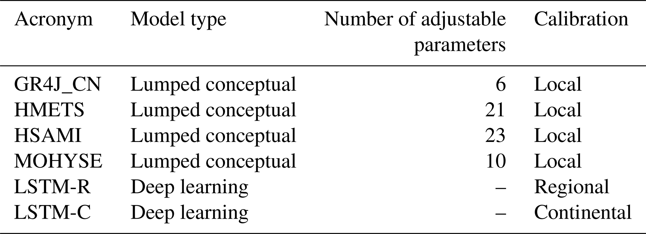
The conceptual lumped hydrological models are compared against an implementation of a long short-term memory (LSTM) model. LSTM models have been used in many applications related to hydrology, from simple rainfall–runoff modelling in single catchments and on regional domains (Kratzert et al., 2018, 2019a), in streamflow forecasting (Girihagama et al., 2022; Sabzipour et al., 2023), and in streamflow prediction at ungauged sites (Arsenault et al., 2023) to name a few. The LSTM model is designed to integrate both dynamic and static features, capturing the temporal patterns of weather variables (e.g. precipitation and temperature) and the intrinsic characteristics of catchments (e.g. drainage area, slope, and land use). The model structure is detailed in the Supplement (Fig. S2), but it is important to note that the model was implemented twice: once using a regional set of catchments (regional model in Table 1; 148 catchments) and the other integrating data from the extra set of 1000 donor catchments to improve training, referred to as the continental model in Table 1 (1148 catchments overall). For both applications, only the amount of input data for training was changed. The structure and hyperparameters remained exactly the same in both instances. A summary of the LSTM model is presented here.

First, the LSTM model ingests data for four dynamic (i.e. time series) variables, namely minimum and maximum daily temperature, as well as rainfall and snowfall. For each streamflow simulation day, a 365 d look-back window of previous meteorological data is used to allow the LSTM model to determine the impact of these data on the streamflow for the simulation day. This block of 365 d × 4 variables is then passed to four LSTM layers each having 256 units. Results are concatenated in two branches and then merged with the static data representing the catchment descriptors. These being static, they are represented by a vector in which each element represents a catchment descriptor. The descriptors are passed into a 128-unit dense layer with a rectified linear unit (ReLU; Agarap, 2018) activation layer. A series of LSTM layers and concatenations is then applied to mimic a part of a residual neural network (ResNET) with residual connections (He et al., 2016; Sarwinda et al., 2021), where shortcuts exist between earlier and later layers. This has led to significant performance gains in other fields, although for applications with much more data and larger LSTM models. As such, to the authors' knowledge, this is the first LSTM-based residual neural network applied in hydrology. Dropout layers are also added throughout the model to increase its robustness and generalizability, given that it is used as a regional model that should consider a wide array of catchments and hydrometeorological conditions for application in climate change scenarios. The final layers in the model are a series of dense layers and activation functions leading to a single output, which is the estimate of the streamflow for the given inputs.

There are key differences in training the LSTM-based model compared to the traditional conceptual hydrological models, particularly in terms of the objective function and the necessity of incorporating a third period of data. The model was then trained using the AdamW optimizer (Loshchilov and Hutter, 2017) with a learning rate that was allowed to change according to the model validation performance, using the Reduce Learning Rate on Plateau (or RLRP) algorithm (Smith and Topin, 2019). To do so, the model compared the simulated streamflow obtained in training with the observed streamflow for each catchment. However, it was necessary to train the LSTM model using data from all catchments at once to ensure that it could learn the relationships between meteorological, geophysical, and hydrologic data in a unique parameterization. Because of this, the objective function is computed on the observed and simulated flows of all catchments. This required normalizing the observed streamflow by dividing it by the catchment area for each catchment in the dataset, ensuring that larger catchments did not outweigh smaller ones in the objective function value. Then, a variant of the Nash–Sutcliffe efficiency (NSE; Nash and Sutcliffe, 1970) was used as an objective function, which was modified to weigh the mean square error (MSE) values for each catchment according to their observed streamflow deviations, as was done by Kratzert et al. (2019b) and repeated with success on the same 148 catchments as in this present study in Arsenault et al. (2023). While slightly different than the objective function used to train the hydrological models, it was deemed satisfactory for three reasons. First, KGE is not an option due to the batching mechanism used during LSTM training, which would compute variability ratios on very small samples (256 in our case). Second, since the LSTM model is trained on all data at once, and the hydrological models are calibrated independently, there needed to be some adjustments to the objective function. Finally, in doing so, we place the LSTM model at a disadvantage as KGE metrics are used to assess performance, meaning the conceptual hydrological models have a slight advantage, making the conclusions more conservative.

The optimization was performed using data from 1981–2002 inclusively (22 years) for training, from 2003 to 2007 inclusively (5 years) for validation, and from 2008 to 2012 (5 years) for testing. This allowed providing sufficient training data for both the regional and extended LSTM models, while allowing enough independent data for comparison and evaluation. It is important to note that the validation period in deep learning is not the same as the validation period for conceptual hydrological models. In deep learning, validation refers to the intermediate evaluation between training epochs and is used as a stopping criterion for model training; thus, it is excluded from both the training and the data scaling/normalization processes. When the validation score stops improving or starts deteriorating for a certain number of consecutive epochs, the model stops training and returns the version with the best validation score. It is then evaluated on the testing period, which is the same as the validation period for conceptual hydrological models. Also, only training data are used for scaling, and then the parameterized scaling function is applied to other datasets to prevent contamination (i.e. training or scaling using data that are out of sample). The list of traditional conceptual lumped and LSTM-based hydrological models used in this study is summarized in Table 1.

Table 1 List of hydrological models used in this study.

2.4 Climate change impacts on hydrological simulations

Two different tests were implemented to evaluate the ability of the conceptual and LSTM-based hydrological models to simulate streamflow in conditions that differ from those in the historical period. The first is a simple sensitivity analysis in which simple delta factors are applied to historical meteorological data. The second uses the more realistic approach of driving the models with bias-corrected climate model simulations. Both methods are presented in this section.

2.4.1 Simple climate sensitivity analysis

A key component of the climate change impact assessment methodology involved conducting a sensitivity analysis to evaluate the impact of hypothetical changes in key climatic variables on streamflow within catchments. This method was designed to evaluate how the conceptual and LSTM hydrological models react to these simple but significant changes in meteorological variables. To achieve this, historical weather data over the entire period was modified by applying predetermined factors to create new datasets that served as rough estimates of future weather conditions. This approach enabled directly assessing the sensitivity of the hydrological system to specific changes in temperature and precipitation, irrespective of the complex dynamics captured by climate models, as will be explored in the next section. Note that no combination of temperature and precipitation changes was used in any of the tests.

The sensitivity analysis included four distinct tests. Two were performed by modifying temperature (i.e. +3 and +6 °C), reflecting potential increases in daily minimum and maximum temperatures. These adjustments were based on the premise that elevated temperatures can significantly impact evapotranspiration rates, snowmelt timing, and ultimately streamflow patterns in catchments. Then, two other tests focused on precipitation (i.e. +20 % and −20 %), recognizing that climate change could increase or decrease precipitation rates depending on the catchment locations and thus alter streamflow peaks and volumes.

2.4.2 Climate models

The second climate change analysis was performed using GCM climate model data to evaluate the differences between conceptual lumped and LSTM-based hydrological models for simulating more complex scenarios than those generated in the sensitivity analysis.

Climate model data

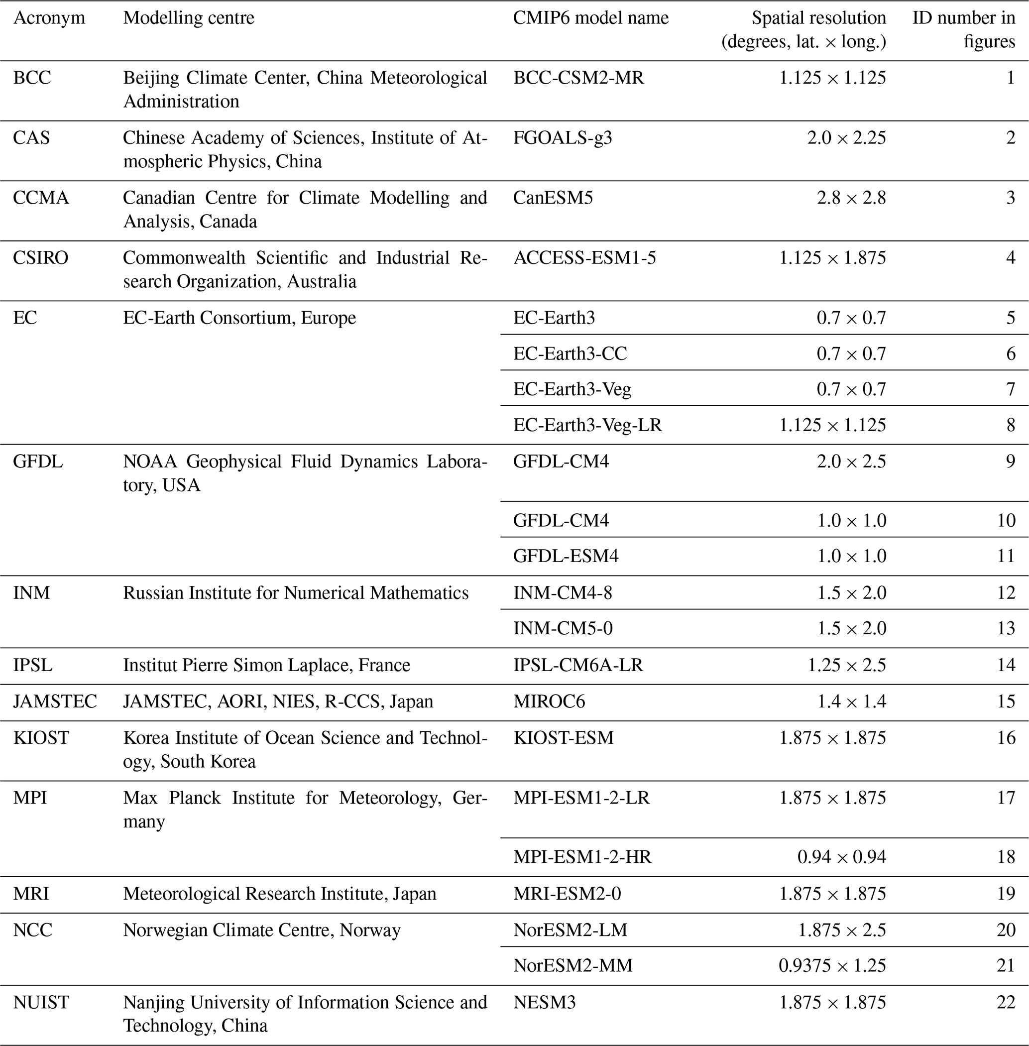
To drive the hydrological models (both conceptual and the LSTM models) with future climate data, GCMs were used. For this purpose, output data from 22 GCMs were downloaded from the Coupled Model Intercomparison Project Phase 6 (CMIP6; Eyring et al., 2016) as shown in Table 2. Availability of the required data was the only factor during model selection. This ensured a broad representation of the current state-of-the-art in climate modelling without any pre-selection bias. As with the historical period simulations, the variables required were maximum and minimum temperature as well as solid and liquid precipitation. This wide array of climate models plays an important role in capturing the range of possible future climate conditions, which allows assessing the robustness of the LSTM-based model compared to the conceptual hydrological models in various future conditions.

Future climate forcings are those of the Shared Socioeconomic Pathway 8.5 (SSP5-8.5; Gidden et al., 2019), a scenario characterized by high greenhouse gas emissions and significant global warming. While acknowledging that SSP5-8.5 represents a pessimistic outlook on future climate change, this scenario was chosen for its utility in maximizing projected climatic changes. This approach is strategic, aiming to reduce the influence of internal climate variability and enhance the discernibility of differences between LSTM-based hydrological simulations and those generated by traditional hydrological models. The integration of scenarios with more pronounced changes aligns with the objective to evaluate the adaptability and predictive power of LSTM models in extreme future conditions.

Table 2 List of the 22 CMIP6 GCM models used in this study.

Climate model data processing

Since it is not possible to calibrate hydrological models or LSTMs on climate model data directly, the GCM data were bias-corrected before being used as inputs to the models. The chosen method, the multivariate bias correction (MBCn) developed by Cannon (2018), stands out for its efficacy in correcting biases across multiple meteorological variables simultaneously. This high-performance correction technique ensures that climate projections maintain statistical properties consistent with the reference datasets, thereby enhancing the reliability of the hydrological assessments. For this study, the reference data were the same as those used for hydrological modelling (i.e. the ERA5 reanalysis data). However, no downscaling of climate data was performed, a decision underpinned by the spatial scale of our hydrological analysis. By aggregating precipitation and temperature data at the catchment scale, we effectively mitigate potential mismatches between the coarse resolution of CMIP6 GCM grids and the finer scales of the catchments. This approach is deemed sufficient despite a portion of the catchments being smaller than the typical resolution of CMIP6 models.

Climate model evaluation period

The bias-correction and climate change simulations were performed on a reference period (1971–2000) and a future period (2070–2099). This design allows for a direct comparison of climate impacts on hydrology under current and projected conditions. However, to accommodate the requisite 2-year warm-up period for the hydrological models, the effective analysis windows are adjusted to 1973–2000 and 2072–2099. This adjustment ensures that the conceptual model states are adequate for accurate simulation, covering 28 years within each period.

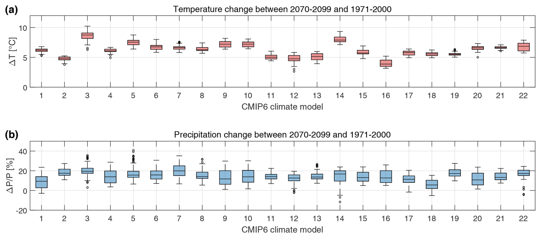
Figure 2 Distribution of the climate change signal for all 148 catchments for the 22 GCMs for mean annual temperature change (future − reference; a) and mean annual total precipitation ([future − reference]$/$reference × 100; b). The future period refers to 2072–2099, while the reference period refers to 1973–2000, inclusively. Each boxplot contains 148 points (i.e. one per catchment).

From Fig. 2, it can be seen that the climate model projections cover a wide range of future conditions, especially in terms of temperatures (Fig. 2a). CanESM5 (model 3) is the warmest GCM (median increase of 8.7 °C), while KIOST-ESM (model 16) is the one with the lowest warming (median increase of 3.9 °C). For most models, the range of the increase in temperature for the various catchments is relatively small, with the widest range being that of CanESM5 (model 3), with approximately 3.9 °C. This indicates that the temperature variability between models is larger than the spatial variability within the study domain. In Fig. 2b, it can be seen that precipitation increases are almost always projected with median increases from 5.6 % in MPI-HR (model 18) to 19.9 % for CanESM5 (model 3). For precipitation, the variability between catchments is higher than the variability between climate models, at least at the climate timescale.

2.5 Evaluation metrics used in this study

In this study, in addition to the KGE and NSE metrics used for model evaluation on the historical period, six streamflow metrics were selected to provide a general overview of the hydrological cycle in future climates: annual mean streamflow (QMA), winter mean streamflow (QMDJF), spring mean streamflow (QMMAM), summer mean streamflow (QMJJA), fall mean streamflow (QMSON), and mean annual maximum streamflow (QMM). The computed metrics specifically target various aspects of streamflow behaviour.

• The annual metric is used to assess the overall hydrological response on a yearly basis, offering insights into long-term changes and trends.

• The seasonal metrics are used to show the temporal distribution of streamflow, allowing for the identification of shifts in hydrological patterns across different times of the year.

• The extreme metric is used for the evaluation of extremes and provides information on potential flooding conditions, which are important for risk assessment and adaptation strategies. However, they are also the most likely to show divergences between methods due to their de facto rarity in datasets, meaning models have fewer examples to learn from than more common streamflow events.

Finally, a third and final general independent metric that was not used as an objective function for training the conceptual models and LSTM models was implemented. This metric is the normalized root mean square error (NRMSE) and is the RMSE normalized by the range of the streamflows in the time series. This allows comparing results between watersheds despite their size differences. It is computed as follows:

$$\begin{array}{}\text{(3)}& \mathrm{NRMSE}={\displaystyle \frac{\sqrt{\frac{\mathrm{1}}{n}{\sum }_{i=\mathrm{1}}^n\left({\left(q_{\mathrm{obs}}^i-q_{\mathrm{sim}}^i\right)}^{\mathrm{2}}\right)}}{max\left(q_{\mathrm{obs}}\right)-min\left(q_{\mathrm{obs}}\right)}},\end{array}$$

where q_obs and q_sim are the observed and simulated flows, respectively, and n is the number of days of data in the evaluation period.

The six streamflow metrics were chosen as they are all reliably simulated by all six hydrological models over the reference period. Low flow and large extremes metrics were not selected as they are less reliably simulated by the hydrological models over the reference period, and, therefore, projecting these metrics in the future comes with larger uncertainty.

3 Results and discussion

This section presents the analysis of results and interprets them within the context of existing literature. We begin with the results related to model calibration, validation, and testing, followed by an interpretation of the sensitivity analysis and an assessment of climate-model-based impacts. Finally, we return to the central question of this paper: which type of hydrological model is more reliable for climate impact studies? The concepts of precipitation elasticity of streamflow and the use of catchment analogues allow us to further deepen this reflection.

3.1 Model calibration, validation, and testing

This section presents the validation/testing results for both the conceptual and LSTM-based hydrological models. First, Fig. 3 presents various performance metrics over the 5-year independent testing period (2008–2012): Kling–Gupta efficiency (KGE), Nash–Sutcliffe efficiency (NSE), relative bias (β), correlation coefficient (r), variance ratio (γ), and normalized root mean square error (NRMSE). The optimal value for each metric is as follows: KGE = 1, NSE = 1, β=0, r=1, γ=1, and NRMSE = 0. Figure S3 in the Supplement presents the results over the calibration (training) period (1983–2002) and shows that the LSTM models outperform the traditional models by a very wide margin, particularly for the LSTM-C. Note that the validation period for the LSTM-based models is not shown as the validation data are contaminated by the training data and, thus, should not be investigated.

Figure 3 (testing period) shows that the LSTM-based models significantly outperform the conceptual hydrological models for the KGE and NSE metrics. Results between the conceptual models are somewhat similar, with GR4J and HMETS leading the pack and HSAMI not far behind in third place. MOHYSE, on the other hand, displays the lowest performance although the median KGE and NSE are still above 0.7 and 0.5, respectively. The LSTM model variants display better scores, with the continental model (LSTM-C) performing better than the regional one. In terms of NSE, the LSTM-C shows a median value of 0.76, whereas the best conceptual model obtains a median value of 0.63. The regional LSTM has a value slightly above 0.71 for comparison. KGE values for the LSTM-C are again significantly better than those of the nearest contender (LSTM-R, 0.80) or the best conceptual model (GR4J, 0.77). Overall, these results indicate that the models were able to simulate streamflow adequately on the 148 catchments and could be used for the remainder of this study, save perhaps the MOHYSE model, whose impacts will be considered in light of these validation results.

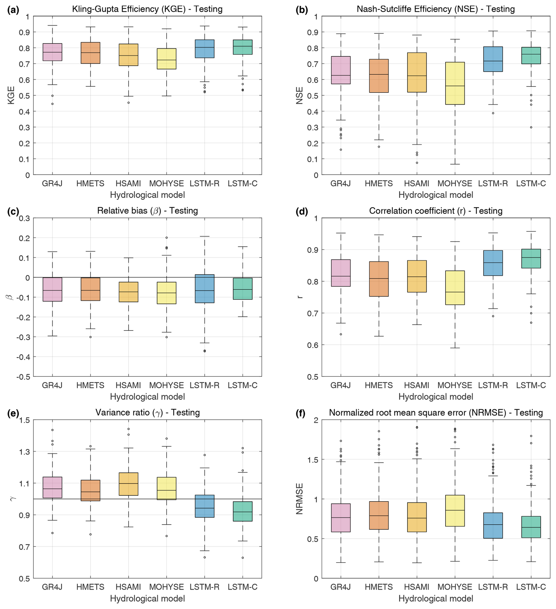
Figure 3 Kling–Gupta efficiency (KGE; a), Nash–Sutcliffe efficiency (NSE; b), relative bias (β; c), correlation coefficient (r; d), variance ratio (γ; e), and normalized root mean square error (NRMSE; f) metrics over the independent 5-year testing period (2008–2012).

To further investigate the source of the gains made by the LSTM models for the KGE metric, Fig. 3c to f present the KGE results for the testing period as decomposed into their individual elements, i.e. relative bias, correlation coefficient, and variability ratio, as well as the NRMSE. It can be seen that the relative bias (Fig. 3c) is similar between models, with more than 75 % of the modelled catchments having a negative bias. The LSTM-R model shows a slightly larger negative bias than the others, and the LSTM-C has the lowest one. The correlation coefficient, on the other hand, clearly shows that MOHYSE lost much of its performance due to its poor correlation coefficient but that both LSTM models scored much higher than the other models for this metric (Fig. 3b). LSTM-C had a particularly large correlation coefficient, with a median correlation coefficient of 0.88, higher than that of the best-performing conceptual model (0.81). Interestingly, the variance ratio (Fig. 3e) shows a striking difference between the conceptual and LSTM-based models. Indeed, the conceptual models tend to overestimate the variability (median values larger than 1), and LSTM-based models tend to underestimate it (median values below 1). In both cases, the over-/underestimation of the median is approximately 10 %. This could be related to the objective function used, as the LSTM training operated on a metric that inherently scaled simulated and observed streamflow by the standard deviation of the observations during its computation, lowering its impact. Conceptual models were calibrated individually using KGE, which has a term specific to variance and is thus directly considered. However, this should favour the conceptual models having better (i.e. closer to 1.0) values of the variance ratios. Finally, the NRMSE (Fig. 3d) shows a slightly smaller relative error for the LSTM models, especially the LSTM-C model. However, differences are not as striking as for correlation or variance ratio. In summary, compared to the traditional hydrological models, the LSTM models have similar bias and slightly lower variability but a much stronger correlation, which suggests a better streamflow timing performance.

In evaluating the six hydrological models, the testing period (equivalent to the validation period for traditional hydrological models) serves as a common independent period for model intercomparison (refer to Fig. 3). Results indicate that LSTM models, particularly LSTM-C, significantly outperform traditional models, as highlighted in recent state-of-the-art papers on LSTM (e.g. Arsenault et al., 2023; Kratzert et al., 2019a; Li et al., 2022), provided they are calibrated with a sufficiently large sample of catchments (Kratzert et al., 2024).

The training period performance of LSTM models, especially LSTM-C, should not be overly emphasized, impressive though it may be. The numerous parameters in LSTM models can and will lead to overfitting if left unchecked. From Fig. S3, it is evident that LSTM training period performance surpasses that of conceptual models. LSTM training scores, such as NSE and KGE, benefit from much better correlation, though variance ratios are slightly lower compared to those of hydrological models, which almost exactly match the levels of variance. There is a broader spread of bias for LSTM, albeit centred at 0. Nonetheless, LSTM models also demonstrate superior performance during the independent testing period, indicating no overfitting despite having many more parameters than traditional hydrological models. LSTM-C, benefiting from data from 1000 additional donor catchments, shows enhanced performance even when tested on the independent period. This indicates the model's ability to leverage additional training catchment data effectively. It underscores the necessity for a large sample size in training to maximize the potential of LSTM models (Kratzert et al., 2024).

LSTMs also excel in utilizing more diverse data types (meteorological and others) than traditional hydrological models. The hydrological models used in this study cannot take advantage of any catchment descriptors, for example. More physically based models could in theory make use of such data. The LSTM implementations discussed in this paper, which only use daily minimum and maximum temperatures, rain, and snow besides the catchment descriptors, represent a fraction of their full potential. Incorporating additional variables would likely improve performance further, albeit at the cost of a decrease in interpretability, increased training resources, and the need for a more flexible model structure with additional nodes to maximize the potential of the added data. This could also enhance the robustness of LSTM models to climate change by constraining outputs more effectively.

However, the complexity of implementing more advanced LSTM models means that all sources of information must also be available for all future time horizons. For instance, employing remote sensing observations (e.g. satellite data) as inputs to LSTM models would likely further improve streamflow simulations for the current period, but such data are not available for future climate change scenarios.

Finally, it should be recognized that not all hydrological models should be considered equal in the interpretation of results. It is quite clear that the continental LSTM model (LSTM-C) clearly outperforms its regional counterpart, from a theoretical and practical point of view. Similarly, the MOHYSE hydrological model is clearly the worst traditional model in this study, from both a performance point of view and based on its simple fully parameterized model structure.

3.2 Sensitivity analysis interpretation

The sensitivity analysis conducted in this study serves as a preliminary approximation, focusing on the expected changes in precipitation and temperature as predicted by GCMs. When looking at Fig. 2, it can be seen that most GCMs' median projected precipitation increase is in the 15 % to 20 % precipitation range, which supports the use of the +20 % scenario. Although the −20 % scenario may not appear realistic over the study area, its use enhances the overall understanding of the model limitations. This approach enabled assessing how the models would react to reductions in precipitation and thus gain deeper insights into their performance in climate change studies. It is also worthwhile to stress that Fig. 2 presents mean projected changes at the annual scale. At the seasonal scale, many GCMs project important decreases in precipitation for certain seasons.

Most median temperature projections among the GCMs ranged between 5 and 8 °C increases, hence the choice of +6 °C. These projections are all from the SSP5-8.5 scenario, which is increasingly seen by many as an overly pessimistic scenario (e.g. Hausfather and Peters, 2020).

Figure 4 shows the expected changes for mean annual streamflow (QMA) for the four sensitivity cases. Results for the five other metrics (QMDJF, QMMAM, QMJJA, QMSON, and QMM) are presented in the Supplement, Figs. S4–S8. In all four scenarios, the four conceptual models behave in a similar way, with small differences depending on the model structure and scenario. However, some divergence is observed in the response of traditional versus LSTM-based models.

The most notable difference is a systematic lower sensitivity of LSTM models to changes in precipitation. When precipitation is altered by adding or subtracting 20 %, the LSTM models generally show smaller changes for all six metrics (Figs. 4 and S4 to S8). The median mean annual streamflow change for a 20 % increase in precipitation is 31.1 % for LSTM-C compared to 35.5 % (GR4J), 34.3 % (HMETS), 33.1 % (HSAMI), and 31.1 % for MOHYSE, with a median average of 33.5 %. The lower sensitivity to precipitation is particularly striking in the spring (Fig. S5) and summer months (Fig. S6), especially for LSTM-C. On the other hand, LSTM models show a larger sensitivity in the winter months (Fig. S4). The LSTM models may incorporate a more nuanced understanding of the hydrological balance compared to the conceptual models, whose change in streamflow is larger than that of the LSTM models for the same variation in precipitation. However, although the results of the LSTM models are different from those of the conceptual models, it is still unclear which of these are more representative of real-world impacts of climate change.

The differences are more nuanced for the temperature increases. For QMA (Fig. 4a and b), LSTM-R and LSTM-C are, respectively, more and less sensitive than the four traditional models for the +3 and +6 °C scenarios. The seasonal sensitivity shows a different pattern, with the LSTM models less sensitive to temperature during spring (Fig. S5) and summer (Fig. S6) but significantly more sensitive during fall (Fig. S7). The LSTM models are also less sensitive to temperature for the QMM metric (Fig. S8). Despite some variability between the different streamflow metrics and across seasons, LSTM models show a different climate sensitivity than that of traditional hydrological models. They are less sensitive to precipitation changes across all metrics. The best-performing LSTM-C model also shows decreased sensitivity to temperature compared to the four traditional hydrological models, with the exception of fall (SON) flows. LSTM-R's increased sensitivity to temperature at the annual scale (Fig. 4) is largely the result of its very large sensitivity for the fall (SON) season (Fig. S7). Its sensitivity tracks that of LSTM-C for the other seasons.

Overall, the LSTM models (and particularly the LSTM-C) exhibit a lower sensitivity to a changing climate compared to the traditional hydrological models. This would suggest that climate change estimates using the traditional hydrological models may be larger than those projected by LSTM models, at least for the streamflow metrics used in this study.

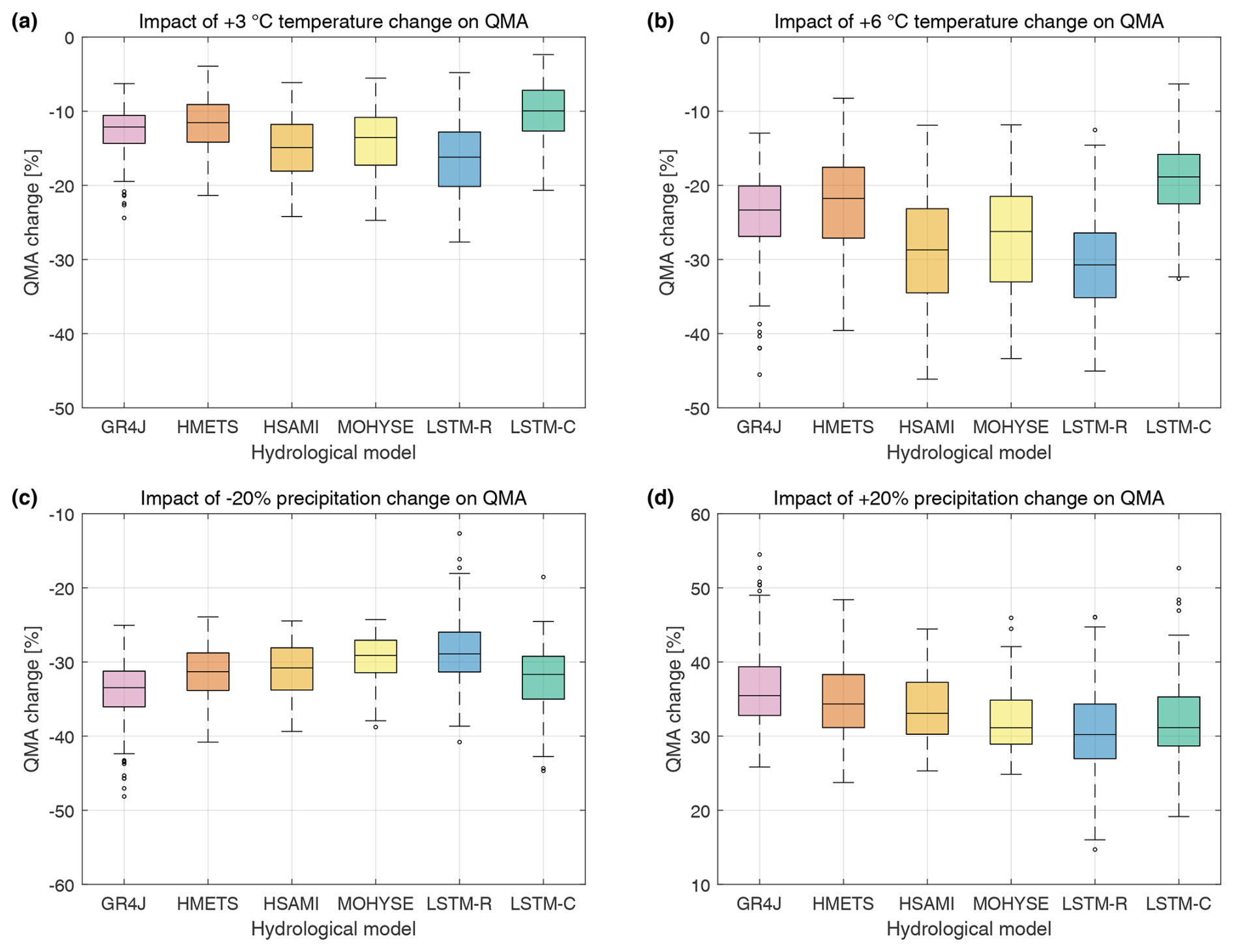
Figure 4 Projected mean annual streamflow (QMA) changes for the four sensitivity scenarios: temperature increase of +3 °C (a) and +6 °C (b) and precipitation relative change of −20 % (c) and +20 % (d).

By independently altering each variable – precipitation and temperature – we were able to quantify the impact of each change, thus avoiding the complication of introducing confounding factors, which is the case when solely relying on GCM simulations for this analysis. This approach provides a clearer understanding of how changes in these variables could impact streamflow, an essential factor in climate change impact assessments. Compared to the hydrological models used in this study, our results show that LSTM models have a lower sensitivity to a changing climate, particularly with respect to precipitation. These observations are useful in the interpretation of streamflow projections obtained from GCM-derived climate scenarios.

3.3 Climate-model-based impact assessment

The sensitivity analysis provided some insights about the traditional and LSTM hydrological model sensitivity to temperature increase and precipitation changes. From Fig. 2, it appears that the SSP5-8.5 scenario corresponds more closely to a combination of the +6 °C and +20 % precipitation sensitivity scenarios. Figure 2 shows that median temperature increases range from +4 to +8.5 °C and from +4 % to +20 % for precipitation. Based on this, the +6 °C and +20 % sensitivity scenarios are more realistic with respect to the SSP5-8.5 scenario than the +3 °C and −20 % ones. Figure 2 also shows that the warmest models also tend to be the wettest, which follows the fundamental principles of atmospheric physics and thermodynamics, with increased evaporation and convection in a warmer climate. The simple sensitivity scenarios did not alter the annual cycles of precipitation and temperature, whereas GCM-derived scenarios present more realistic but also more complex future projections.

Figure 5 presents combined projected changes for all six streamflow metrics and six hydrological models. Each boxplot represents the distribution of 3256 values, 1 for each combination of 148 catchments and 22 GCMs. Results show that LSTM models tend once again to behave differently than the four traditional hydrological models and in a manner consistent with some of the observations made from the simple sensitivity studies. In particular, we can note the following features:

• For mean annual streamflow (QMA), the LSTM models project future changes similar to that of the traditional models. There are, however, significant changes at the seasonal scale.

• LSTM models project smaller flow decreases in winter (DJF), spring (MAM), and summer (JJA) compared to the traditional hydrological models.

• LSTM models project much larger streamflow decreases during the fall (SON).

A Wilcoxon signed-rank test was used to test for statistical differences between the LSTM-based models and the conceptual hydrological models. LSTM-based models are statistically different than all other models in all cases except the following:

• Fig. 5a (QMA) – LSTM-R is not statistically different from HSAMI and LSTM-C is not statistically different from GR4J;

• Fig. 5e (QMJJA) – LSTM-R and LSTM-C are not statistically different from HSAMI.

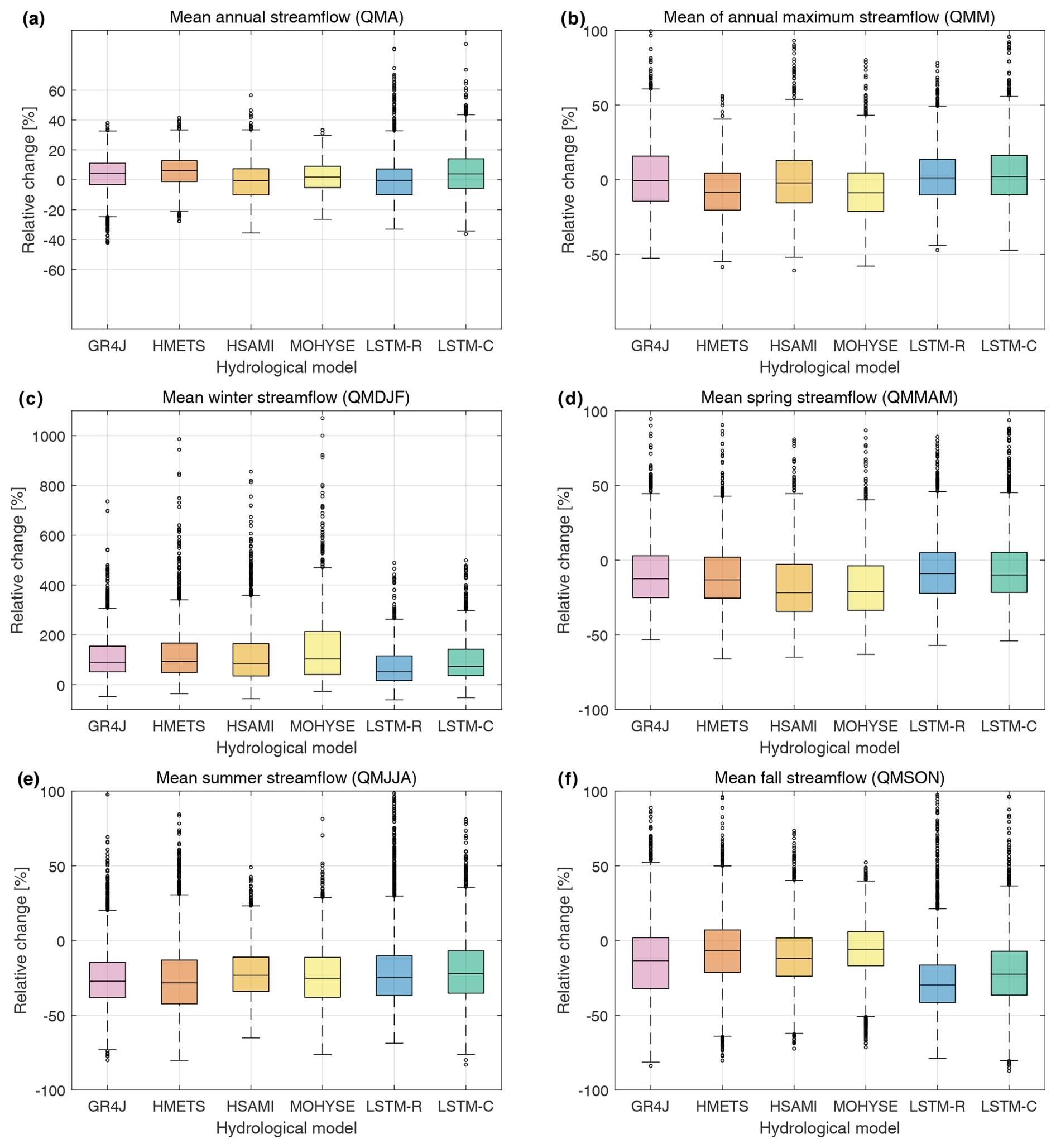
Figure 5 Boxplots of the range of expected change for all six streamflow metrics. The boxplots are aggregations of the 22 GCMs and 148 catchments. The boxplots are thus drawn from a distribution of 3246 points (148 catchments × 22 GCMs). Note that the y-axis range is different in panel (c) than the others due to the much larger values for this period.

One objective of this study is to look at the climate sensitivity of hydrological models, which is how their future streamflow response depends on forcing-induced changes in climate variables at (for precipitation) or near (2 m height for air temperature) the surface. In order to do so, we have looked at the differential response of all six hydrological models to the following combinations of six contrasted climate models: (1) hot vs. cold, (2) high vs. low precipitation scaling, and (3) wet vs. dry models. Precipitation scaling evaluates the sensitivity of precipitation change to an increase to temperature. Here, precipitation scaling is simply the increase percent (%) in mean annual precipitation divided by the mean annual temperature increase. The median changes between both pairs of three climate models are outlined below.

• 1.

  Hot vs. cold climate models.

  • The three hottest models are CanESM5 (model 3: +8.75 °C), IPSL (model 14: +7.90 °C), and EC-Earth3 (model 5: +7.55 °C).

  • The three coldest models are KIOST-ESM (model 16: +3.88 °C), INM-CM4-8 (model 12: +4.76 °C), and FGOALS-g3 (model 2: +4.80 °C).

• 2.

  Highest vs. lowest precipitation scaling climate models.

  • The three highest scaling models are FGOALS-g3 (model 2: +3.65 % °C⁻¹), KIOST-ESM (model 16: +3.28 % °C⁻¹), and MRI-ESM2-0 (model 19: +3.12 % °C⁻¹).

  • The three lowest scaling models are MPI-ESM1-2-LR (model 17: +1.00 % °C⁻¹), BCC-CSM2-MR (+1.5 % °C⁻¹), and NESM3 (model 20: +1.62 % °C⁻¹).

• 3.

  Wet vs. dry climate models.

  • The three wettest models are EC-Earth3-Veg (model 7: +19.9 %), CanESM5 (model 3: +19.4 %), and FGOALS-g3 (model 2: +17.5 %).

  • The three driest models are MPI-ESM1-2-LR (model 17: +5.6 %), BCC-CSM2-MR (model 1: +9.3 %), and NESM3 (model 20: +10.7 %).

The results are presented in Fig. 6 for mean annual streamflow (QMA). Figure 6 shows the changes (in percentage) between both contrasted groups for all six hydrological models. For example, for the hot vs. cold model test, a value of −10 % indicates that mean annual streamflow is 10 % smaller for the three hottest models compared to the three coldest ones (corresponding, for example, to a 5 % increase for the hot models and a 15 % increase for the cold ones). Each boxplot of Fig. 6 is therefore made of 148 × 3 values, corresponding to the number of catchments and climate models. The median results are shown in Table 3.

Results do not show large differences in terms of annual climate sensitivity. This applies both to the traditional hydrological model group and when comparing the LSTM models to the traditional ones. The LSTM models show a larger sensitivity to temperature and precipitation scaling (Fig. 6a and b). The differences are less striking than for the sensitivity analysis, and this is likely because hot models also tend to be wet as discussed above.

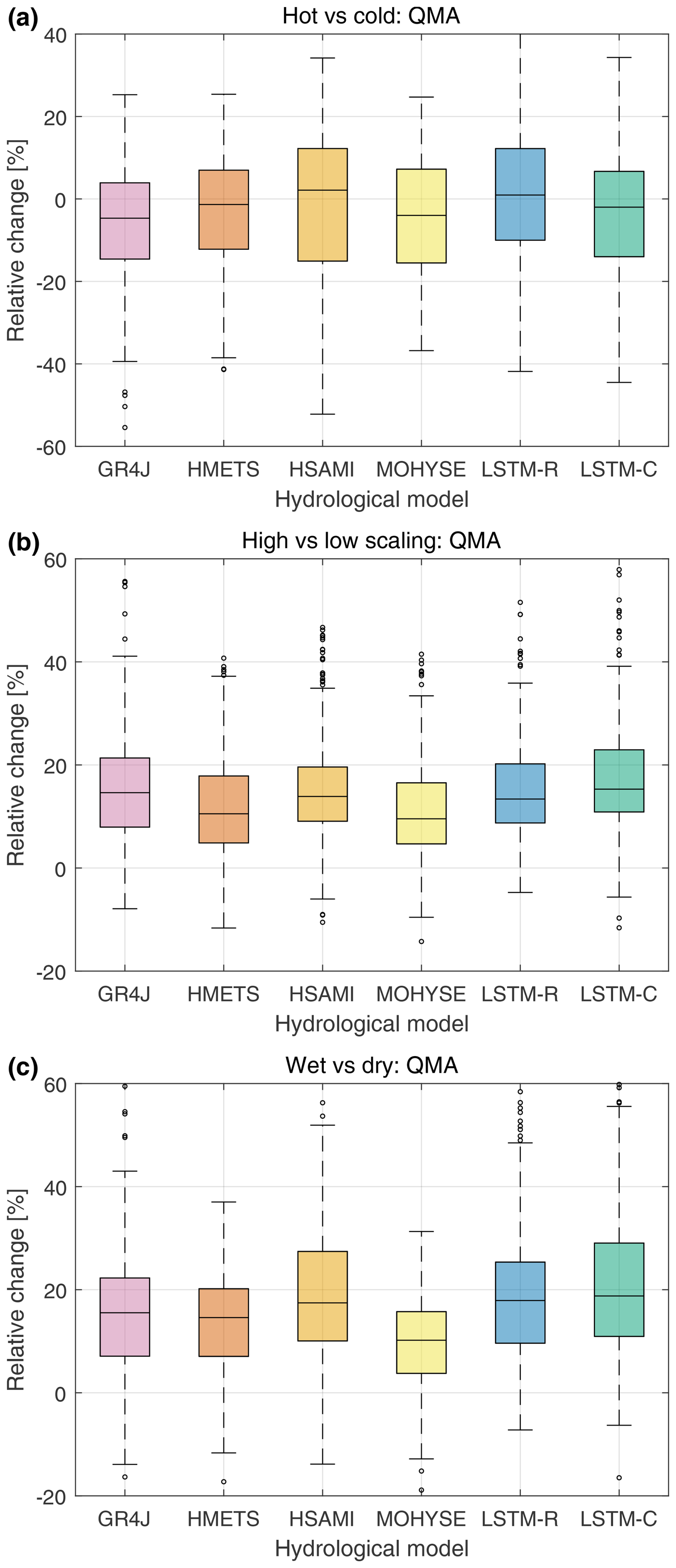
Figure 6 Boxplots of percent (%) change between two groups of three contrasted climate models: (a) hot vs. cold models, (b) high vs. low precipitation scaling models, and (c) wet vs. dry models. The boxplots are drawn from a distribution of 444 points (148 catchments × 3 climate models).

Table 3 Median results from Fig. 6, indicating percent (%) change between two groups of three contrasted climate models.

This analysis, based on climate model projections, integrates the temporal dynamics between variables, compared to sensitivity analysis, which preserves the historical timing of events. This more complete picture provides details on transformations in hydrological indicators under climate change and allows for comparing the conceptual and LSTM-based models under these conditions.

The analysis showed that the results were generally consistent with those of the sensitivity analysis but were not as contrasted, likely due to the combination of precipitation and temperature changes that tend to compensate for one another in the LSTM models. An important objective of this paper was to investigate the climate sensitivity of hydrological models. The climate sensitivity of traditional hydrological models mostly comes from model structure and complexity but also from parametric uncertainty. The four traditional hydrological models share similar structures, all being lumped conceptual models. Within that group, model complexity varied significantly, especially with respect to snow and evapotranspiration models, ranging from extremely simple parametric formulas (MOHYSE) to more complex formulations such as the HMETS snow model. Based on these considerations, it was perhaps surprising to observe that climate sensitivity was relatively similar across all six hydrological models. The LSTM models did show a larger sensitivity to temperature in the hot/cold model experiment. LSTM models also showed a larger sensitivity to high vs. low precipitation scaling but not when looking at the wet/dry model experiment. All four traditional hydrological models were similar in their climate sensitivity, and even the simple MOHYSE model was not an outlier for the six streamflow metrics considered, which tends to demonstrate the robustness of the results. It is important to note that the climate sensitivity experiment only looked at the mean annual streamflow metric. No effort was made to sideline some of the climate models that have high climate sensitivity, also known as hot models (e.g. Hausfather et al., 2022; Kreienkamp et al., 2020; Rahimpour Asenjan et al., 2023).

3.4 The main question: which type of hydrological model should we trust more for climate change impact studies?

This is ultimately the most important question but also the most difficult one to answer. Since there are no future streamflow data available, we are mostly left with theoretical arguments. One way to navigate this issue is simply to state that these LSTM models should be included in multi-model ensembles to better assess modelling uncertainty (e.g. Dams et al., 2015; Najafi and Moradkhani, 2015). However, many studies suggest that we should have more confidence in hydrological models that yield better results in the historical period, as they are better at representing processes (e.g. Krysanova et al., 2018), which leads back to the initial question: which type of model should we trust more? Based on this sole consideration, LSTM methods should be favoured. Nonetheless, no matter how appealing the argument, relying solely on model performance over the historical record falls short in a few aspects. The concept of the death of stationarity (e.g. Galloway, 2011; Milly et al., 2008) tells us that past hydrological behaviour is not a reliable indicator of future conditions, meaning that a model calibrated solely on historical data might not accurately capture future dynamics. As discussed above, all hydrological models are somewhat parameterized, even the most physically based ones, and there is no guarantee that the climate sensitivity of these parameterizations is adequate.

The observation that all six hydrological models display an overall somewhat similar climate sensitivity is perhaps comforting, for example, by telling us that all existing climate change impact studies are not obsolete, but also perhaps premature, as our analysis did not examine this in much detail, and, clearly, a more detailed seasonal analysis looking at more streamflow metrics is warranted. Still, there is an argument to be made that the continental LSTM-C model is the best fit for climate change studies. The inclusion of 1000 additional catchments, mostly located in a warmer climate, indicates that LSTM-C should have, at the very least, a theoretical advantage over single-catchment or local models. It has learned the complex relationship between climate variables and streamflow, not only over the study domain but also from 1000 catchments, many of which are representative of, and even warmer than, the expected end-of-century climate over the study domain. Other types of hydrological models (regional, distributed, and more physically based models) can also make use of some aspects of this trove of data (more catchments, more meteorological variables), but they still face the problem of stationarity: model parameters are still fixed in time, and thus the model cannot account for non-stationarity in the same way the LSTM models can. LSTM models are particularly fit at capturing the complex, non-linear climate interactions leading to streamflow due to this large-scale training and exposure to various climates. They may, therefore, be better at capturing the temporal dynamics of hydrological processes and their sensitivity to long-term changes in climate patterns. However, the LSTM model process representation is quite challenging and obfuscated, meaning it cannot easily be probed directly to assess how the hydrological cycle is modelled. This is a limitation, as it is currently very difficult or nearly impossible (depending on the model complexity) to assess this in an LSTM-based model, which means it requires more blind trust than conceptual models.

When it comes to extreme or rare events, it is likely that the training dataset contains too few of these events, leading to more doubtful performance compared to conceptual models. In such cases, traditional hydrological models may still be better, despite other weaknesses. For example, the parameter sets of conceptual hydrological models are fixed during the calibration period with the hypothesis that these are constant over time (e.g. seasonally). However, this has been shown to be inaccurate (e.g. Kim et al., 2015; Mendoza et al., 2015; Bérubé et al., 2022), and LSTM-based models are not constrained to these same processes and can learn to modify streamflow patterns according to hydrometeorological conditions through their immense number of internal weights. Nonetheless, beyond theoretical arguments, there are ways to practically investigate hydrological model fitness. Several authors (e.g. Bérubé et al., 2022; Krysanova et al., 2018; Roudier et al., 2016; Todorović et al., 2022) have suggested approaches using historical data to assess hydrological model fitness for climate change impact studies. While these approaches offer interesting insights, hydrological variability over the recent historical record remains small compared to expected changes by the end of this century (Bérubé et al., 2022), and it is therefore extremely difficult to assess the true sensitivity of hydrological models to climate change simply using historical data. We therefore looked at two different ways of assessing hydrological model sensitivity: precipitation elasticity of streamflow and climate analogues.

3.5 Precipitation elasticity of streamflow

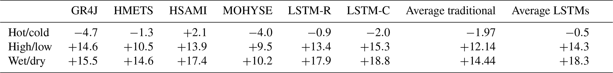
One metric that can be used to assess the sensitivity of streamflow to precipitation is the precipitation elasticity of streamflow index, which is defined here as the change in mean annual streamflow divided by the change in mean annual precipitation. For example, an elasticity of 0.5 means that for every change of 1 % in precipitation, streamflow responds with a change in the same direction of only 0.5 % (Schaake, 1990). Precipitation elasticity is not easily computed, but in the case of our +20 % precipitation increase sensitivity scenario, it is easy to do since only precipitation is changed (temperature is constant), and we do not have to account for co-dependencies between precipitation, temperature, and streamflow. Results in Fig. 4c and d showed significant disparities in how both types of hydrological models (conceptual and LSTM-based) handled changes in precipitation volumes. Figure 7 shows the spatial distribution of precipitation elasticity for all tested models (traditional and LSTM-based). It can be seen that precipitation elasticity is smaller for both LSTM models (median values of 1.51 and 1.55 for LSTM-R and LSTM-C) compared to values of 1.77, 1.72, and 1.65 for the three best traditional hydrological models (GR4J, HMETS, and HSAMI, respectively). The simplest model (MOHYSE) is more in line with the LSTM estimates.

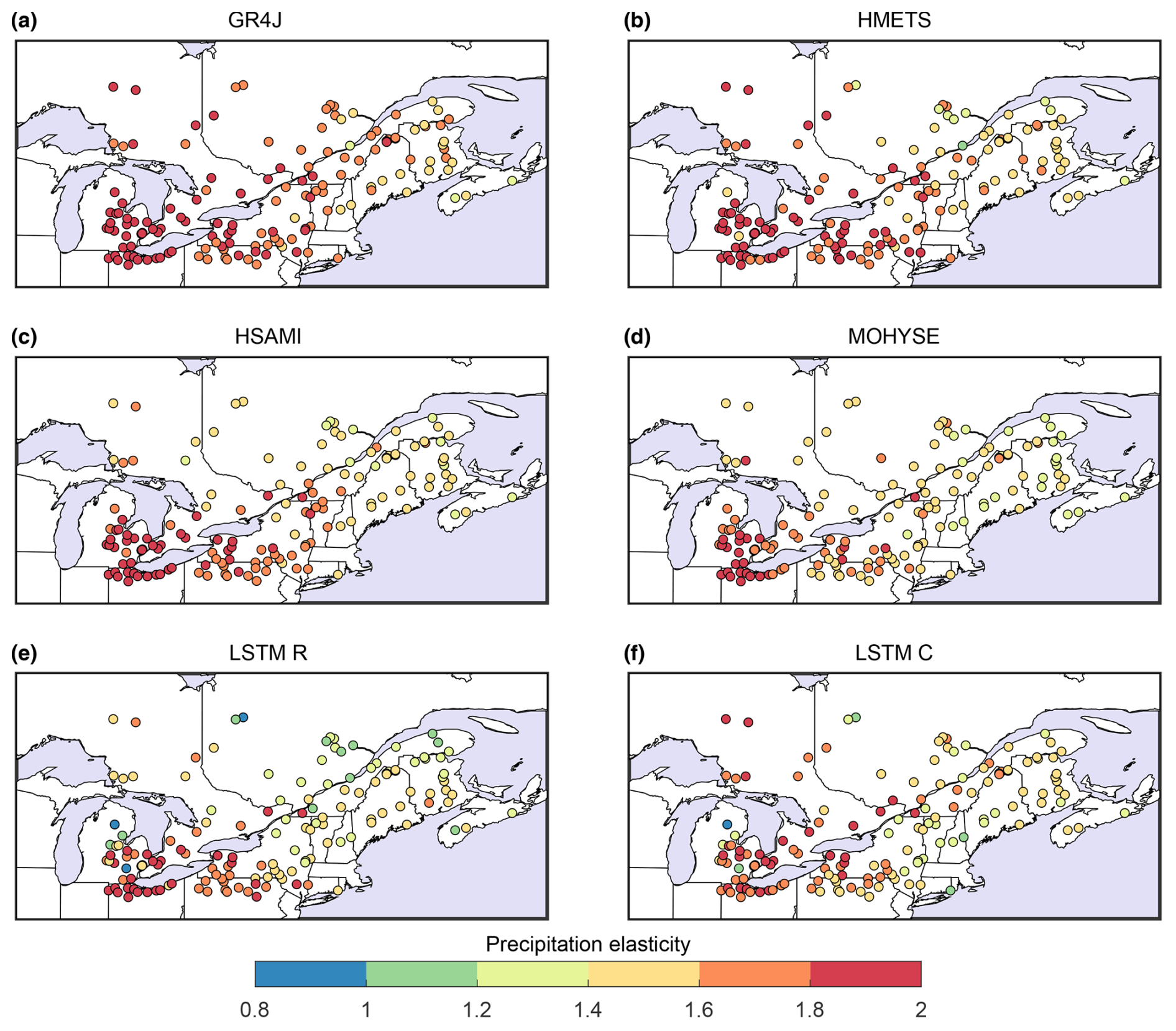
Figure 7 Rainfall elasticity for each of the 148 catchments as evaluated by the six hydrological models.

Precipitation elasticity can be used as a metric to assess how each model type compares to values obtained from the literature (Maharjan et al., 2022). This analysis has one major caveat in that it considers the same temporal pattern of precipitation but with modified amplitude. This is a simplistic representation of the precipitation drivers and processes, but, nonetheless, it allows comparing the obtained values to established precipitation elasticity of streamflow values in the literature to validate plausible ranges.

Chiew et al. (2006) provide an estimate of precipitation elasticity of streamflow for catchments throughout the world, using the median elasticity of all available years of data for a set of over 500 catchments worldwide. Overall, their study shows that elasticity values ranging between 1.0 and 3.0 are reasonable, with values below 2.0 being more representative of colder, higher-latitude catchments such as those in this study. Twenty catchments of Chiew's (2006) study are within our study zone, and all but one (95 %) have precipitation elasticity below 2, compared to 76 %, 82 %, and 83 % for GR4J, HMETS, and HSAMI, respectively, compared to 89 % and 92 % for LSTM-R and LSTM-C. In addition, 75 % of Chiew et al. catchments have values below 1.5. This compares to 7 %, 16 %, and 23 % for GR4J, HMETS, and HSAMI, respectively, and 48 % and 37 % for both LSTM models. Our estimates are slightly larger than that of Chiew et al. (2006), but both LSTM models provide the ones that are closest. Sankarasubramanian et al. (2001) also provided estimates in a large-sample US study. Their estimates are smaller than that of Chiew et al., but they used a different methodology that underestimates values for catchments with significant snowfall, which is the case for most catchments within our study domain. This shows that estimating precipitation elasticity is not a straightforward task. Zhang et al. (2022) recommend using decadal time steps to assess the elasticity, which is more in line with what was performed in this study. Overall, the precipitation elasticity values obtained in this study are lower for LSTM models and are consistent with the lower sensitivity to precipitation observed earlier. Our estimates are slightly larger than that of the literature but are much closer for the LSTM models.

3.6 Catchment analogues

One additional way to quantitatively assess the climate change fitness of hydrological models is to examine how the six hydrological models perform on analogue catchments. This was done for all of the 148 target catchments and for all 22 GCM future climate scenarios. In all cases (for each single catchment and each given climate model), we look for catchments within the 1000-donor group that had similar annual precipitation and temperature cycles to that of the target catchment in the future. The best 10 analogues out of 1000 were selected, based on Euclidean vectors composed of the following values: mean annual temperature, mean annual precipitation, catchment areas, 12 monthly mean temperatures, and 12 monthly mean total precipitations. Equal weighing was used for each of those 27 values in order to find the best analogues. It was decided not to use any physical catchment descriptors (e.g. land cover) as this would likely favour the LSTM models, which can make explicit use of such descriptors. The future streamflow computed by each hydrological model over the target catchment was then compared to the mean streamflow of all 10 chosen analogues over the reference period. All streamflow hydrographs were normalized to a unit area to account for catchment size mismatch. Figure 8 shows typical results from this procedure. It shows the annual mean hydrographs for all six hydrological models for catchment 140 and climate model 16, superimposed on the envelope of mean streamflow hydrographs from the 10 closest analogues. It also shows the target catchment location (red circle) as well as the 10 closest analogues (blue circles). Figure 8 shows that there is a large disparity in performance among hydrological models, especially in the spring and fall.

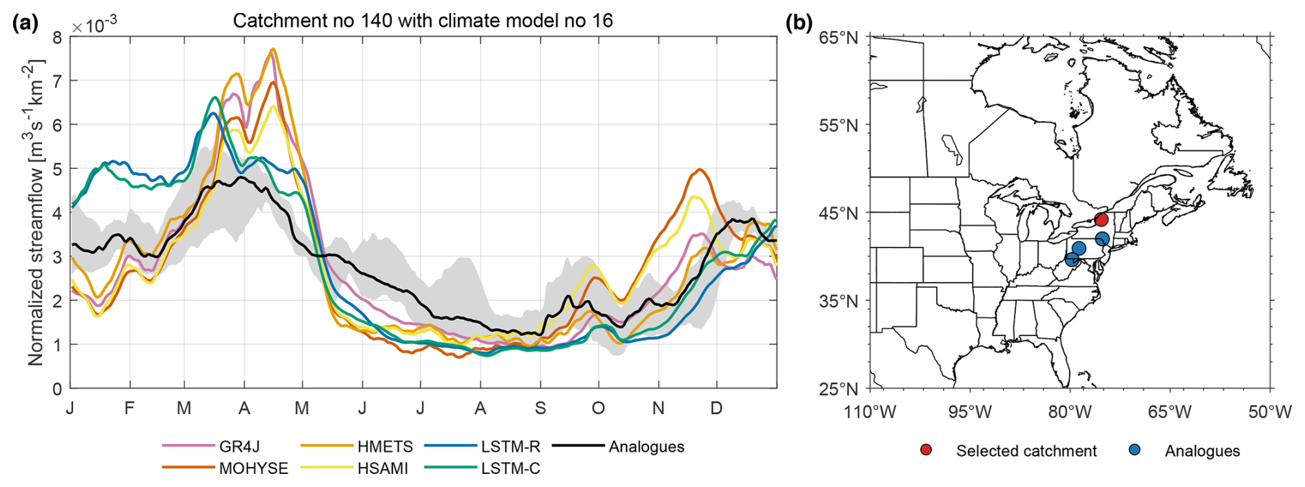
Figure 8 (a) Mean annual streamflow hydrographs for catchment 140 projected by climate model 16. The hydrographs are superimposed over the shaded area of the 10 closest analogue catchments from the 1000-donor population. (b) Location of target catchment (red circle) and the 10 closest analogues (blue circles).

In order to extend the analysis of Fig. 8 to all catchments and provide a more quantitative assessment, the root mean square difference between the normalized annual streamflow hydrograph (NRMSE) of each hydrological model and the mean of the 10 analogues was computed for all catchments and all climate models, for a total of 3256 test cases (148 target catchments × 22 climate model projections). The results are shown in Fig. 9. The results show that LSTM-C provides on average the best streamflow estimates for the analogues, having a statistically significant lower median NRMSE than all other models. LSTM-R is second best. Amongst the four traditional hydrological models, GR4J performs the best although differences are small. Figure S7 decomposes the results of Fig. 9 into the four seasons for a more detailed picture. It shows that LSTM-C's better performance comes mostly from the winter and spring seasons.

Figure 9 NRMSE difference between the annual mean hydrograph and the mean of the 10 closest analogue catchments out of the 1000-donor population. The boxplots are drawn from the 148 NRMSE values, 1 for each catchment. Each catchment value represents the average across all 22 GCMs. Seasonal performance is presented in Fig. S7.

Figured S8 presents annual results (same as Fig. 9) for all 22 GCMs separately. They show that the conclusions are quite consistent across all GCMs, although the advantage of both LSTM models varies depending on the considered GCM. A peculiar observation is that both LSTM models perform worst for GCMs 12 and 13, which are two versions of the same GCM (INM4.8 and INM5.0). A deep look at the climate projections of the INM GCM over the study domain would probably show that it likely projects outlier climate projections amongst our chosen 22-member GCM ensemble. Like all analogue approaches, success depends on the ability of finding proper analogues. Nonetheless, results show that both LSTM approaches are consistently better at matching observed mean annual streamflows for the chosen analogues. The differences are not large but are statistically significant.

As mentioned above, the NRMSE differences shown in Figs. 9, S7, and S8 are relatively small for each of the 3256 test cases. Each of the six hydrological models was ranked from 1 (smallest root mean square error; RMSE) to 6 (largest). Figure 10 presents the ranking results. Results are similar to that of Fig. 9 but with larger separation between the boxes. This emphasizes the consistency of LSTM-C at being the best hydrological model for the analogue catchments due to the somewhat relatively small RMSEs.

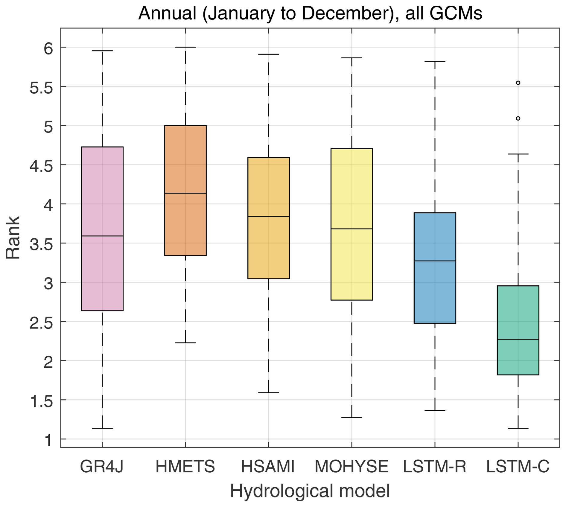
Figure 10 Average performance ranking from 1 (best) to 6 (worst) of six hydrological models at reproducing the mean streamflow hydrograph from the 10 best analogues out of the 1000 donor catchments. The boxplots are made of 148 values (1 for each catchment) and represent the mean ranking across the 22 GCMs.

The analogue approach, as used in this study, faces several limitations. It is based solely on precipitation, temperature, and area, without considering other variables. This limitation makes it difficult to find perfect analogues for the study areas. Even small differences in precipitation and temperature, which might seem negligible when selecting analogues, can lead to significant differences in streamflow. Despite these limitations, the approach conclusively demonstrates that hydrological models exhibit significant differences in their ability to generate streamflow on analogue catchments and that the continental LSTM appears best-fitted for climate change impact studies.

4 Conclusion

This study compared four traditional hydrological models against two LSTM-based models across a domain of 148 catchments, focusing on projecting future streamflow. One LSTM model (LSTM-R) was trained exclusively on the study domain, while the other (LSTM-C) included 1000 additional catchments from a broader range of climate zones. The climate sensitivity of all six models was evaluated using four simple climate change scenarios (+3, +6 °C, −20 %, and +20 % precipitation change) and 22 CMIP6 climate projections under the SSP5-8.5 scenario.

The first objective of this paper was to assess the performance of LSTM-based hydrological models in climate change impact studies. Results showed that both LSTM models clearly outperformed the four traditional hydrological models during the reference testing periods. Annual-scale streamflow projections from the LSTM models were relatively similar to those of the traditional models, demonstrating that LSTM models can be effectively used for hydrological impact studies and provide realistic streamflow projections.

The second objective was to compare future streamflow projections from the LSTM models with those obtained from conventional hydrological models, aiming to identify differences across various streamflow metrics and multiple catchments. Despite similarities between all models at the annual scale, there were notable differences at the seasonal scale between the four traditional models and the two LSTM models. In most cases, the differences between the two model classes (traditional vs. LSTM) were larger than those within models of the same class, indicating that LSTM models differ in climate sensitivity compared to traditional hydrological models.

The third and final objective of the paper was to explore the climate sensitivity of both model classes in greater detail. Results showed that LSTM models exhibited reduced sensitivity to precipitation changes compared to traditional models, and this reduced sensitivity was consistent across all streamflow metrics and seasons. LSTM models also showed slightly reduced sensitivity to temperature changes at the annual scale, with variability depending on the metric and season. For example, for mean flows, the LSTM models projected smaller changes in winter, spring, and summer streamflow but much larger decreases in fall. Overall, the results suggest that traditional hydrological models exhibit greater climate sensitivity than LSTM models and may overestimate future streamflow changes, at least for the streamflow metrics considered in this study.

From a theoretical perspective, LSTM models, particularly LSTM-C, appear to be the most suitable. LSTM-C outperformed all other models during the reference period, a widely considered critical factor for climate change studies. Additionally, LSTM-C was trained on a larger dataset of catchments from diverse climate zones, ensuring sufficient climate information to remain in interpolation mode, even under extreme future climate scenarios. In contrast, all other hydrological models, especially the traditional ones, operate in extrapolation mode for climate change studies, relying on climatic inputs not encountered during their calibration or training periods.

The theoretical advantage of LSTM models was further quantified by demonstrating that the rainfall elasticity obtained from both LSTM models was lower than that of traditional hydrological models (consistent with the observed reduced sensitivity to precipitation). More importantly, these elasticity values aligned with estimates from other studies conducted over the same study domain. Furthermore, both LSTM models consistently outperformed traditional models in predicting streamflow for analogue catchments approximating future climate conditions of the 148 target catchments.

Our findings strongly support the use of LSTM models for hydrological climate change studies. Transitioning to LSTM models, however, requires careful consideration of their data requirements, their computational complexity, and the interpretability of their projections. This highlights the need for ongoing research and methodological advancements in hydrological modelling within the context of climate change. Nevertheless, the role of traditional hydrological models in climate change studies is far from obsolete. While LSTM-based models appear better suited for such studies, the future streamflow projections from both model types were often similar, and the quantitative advantages of LSTM models over the best-performing traditional model were sometimes modest.

Further research is essential to fully explore the potential benefits of LSTM-based models, particularly for catchments in different climate zones and their effects on streamflow extremes, which are critical for many adaptation strategies. Additionally, process-based hydrological models should be given more consideration, as they may, at least theoretically, be better suited to climate change impact studies than the simpler models used in this study.

Finally, the potential impacts of climate change extend beyond the six streamflow metrics analysed here. Future research should consider annual and seasonal extremes, as well as changes in seasonal and interannual variability, which are hallmarks of a changing climate.