the Creative Commons Attribution 4.0 License.
the Creative Commons Attribution 4.0 License.
 | 23 Feb 2024
Flow intermittence prediction using a hybrid hydrological modelling approach: influence of observed intermittence data on the training of a random forest model
Annika Künne
Flora Branger
Sven Kralisch
Alexandre Devers
Jean-Philippe Vidal
Rivers are rich in biodiversity and act as ecological corridors for plant and animal species. With climate change and increasing anthropogenic water demand, more frequent and prolonged periods of drying in river systems are expected, endangering biodiversity and river ecosystems. However, understanding and predicting the hydrological mechanisms that control periodic drying and rewetting in rivers is challenging due to a lack of studies and hydrological observations, particularly in non-perennial rivers. Within the framework of the Horizon 2020 DRYvER (Drying River Networks and Climate Change) project, a hydrological modelling study of flow intermittence in rivers is being carried out in three European catchments (Spain, Finland, France) characterised by different climate, geology, and anthropogenic use. The objective of this study is to represent the spatio-temporal dynamics of flow intermittence at the reach level in mesoscale river networks (between 120 and 350 km2). The daily and spatially distributed flow condition (flowing or dry) is predicted using the J2000 distributed hydrological model coupled with a random forest classification model. Observed flow condition data from different sources (water level measurements, photo traps, citizen science applications) are used to build the predictive model. This study aims to evaluate the impact of the observed flow condition dataset (sample size, spatial and temporal representativity) on the performance of the predictive model. Results show that the hybrid modelling approach developed in this study allows the spatio-temporal patterns of drying to be accurately predicted in the three catchments, with a sensitivity criterion above 0.9 for the prediction of dry events in the Finnish and French case studies and 0.65 in the Spanish case study. This study shows the value of combining different data sources of observed flow condition to reduce the uncertainty in predicting flow intermittence.
- Article
(6289 KB) - Full-text XML
-
Supplement
(8831 KB) - BibTeX
- EndNote


River systems are an essential link in terrestrial biodiversity. They constitute the habitat of many animal and plant species within the riverbed and in the riparian zone (Leigh and Datry, 2017). They also serve as ecological corridors by providing a connection between upstream and downstream areas for mobile species and by transporting nutrients and sediments necessary for the survival of species located downstream (Deiner et al., 2016). In particular, ecologists assume that intermittent rivers are biodiversity hotspot thanks to the succession of different flow phases (e.g. flowing, isolated pools, dry) which promotes species richness (Datry et al., 2014).
By impacting the hydrological cycle and increasing the risk of drought (Gudmundsson and Seneviratne, 2016; Tramblay et al., 2021), climate change threatens river biodiversity (Bond et al., 2008). Prolonged drying and shifting of river sections from perennial to intermittent flow can endanger ecosystems and limit the access to water resources useful to our society (Steward et al., 2012; De Girolamo et al., 2017; Tonkin et al., 2019).
The term “intermittent rivers” refers to all rivers with a non-perennial flow. This includes ephemeral rivers with short periods of flow in direct response to rainfall or snowmelt events, rivers with seasonal flow, and nearly perennial rivers with infrequent periods of drying (Buttle et al., 2012; Snelder et al., 2013; Shanafield et al., 2021). In this study, the term “flow intermittence” will refer to the alternation between flowing phases and phases with interrupted flow (completely dry riverbed or disconnected pools).
Although they represent a large proportion of terrestrial rivers (Messager et al., 2021), intermittent rivers are still poorly known (Acuña et al., 2014; Meerveld et al., 2020; Fovet et al., 2021), and their study in hydrology is relatively recent. Modelling the hydrological functioning of drying river networks (DRNs) can help understand the impact of drying on ecosystems and predict the evolution of the drying spells and possible tipping points in flow regimes under climate projections.
Studies have already looked at modelling intermittent rivers with a physical hydrological model (Jaeger et al., 2014; Tzoraki et al., 2016; Llanos-Paez et al., 2023). One major difficulty in modelling flow intermittence is that hydrological models have difficulties in simulating zero flows (Shanafield et al., 2021). First there is a numerical challenge: the flow routing scheme implemented in the models to propagate the streamflow across the river networks cannot represent sudden transitions from wet to dry. Second, the origins of intermittence are multiple (disconnection between the river and the water table, drying up following a long period without precipitation, infiltration from the riverbed into a fault or a karstic subsoil, drying up following anthropic withdrawals, etc.) (Datry et al., 2016) and sometimes very local. Representing all these processes in the models is thus complex and requires a large amount of data. A more common approach to modelling intermittent rivers is the use of artificial neural networks (ANNs) (Daliakopoulos and Tsanis, 2016; Beaufort et al., 2019) and random forest (RF) (González-Ferreras and Barquín, 2017; Beaufort et al., 2019; Belemtougri, 2022; Jaeger et al., 2023) models. These models are easier to implement, do not require a priori knowledge of the origins of drying, and show good performances in predicting the spatial distribution of flow regimes (perennial or intermittent) in the river networks. The covariates used to predict the river flow regime are usually the stream physical characteristics (width, length, slope, geological context, etc.) and climate variables such as precipitation, temperature, and evapotranspiration. Predicting the spatial and temporal dynamics of drying in intermittent river systems requires providing the RF models with additional covariates on the spatialised hydrological conditions along the river systems at a sufficiently fine time step and fine spatial resolution. This can be achieved using spatially distributed hydrological models at a daily or smaller time step.
Another challenge in the study of intermittent river networks is to collect observed data of flow intermittence to train or validate the models. Studies of river intermittence on a large scale mainly use gauging station data (Belemtougri, 2022; Messager et al., 2021; Tramblay et al., 2021; Beaufort et al., 2019; Reynolds et al., 2015). Gauging station data are easy to retrieve and analyse and have the advantage of providing data at a regular time step over long periods. But stations are mainly located on rivers with perennial flow (Eng et al., 2016; Meerveld et al., 2020), and their spatial distribution is not dense enough to understand the flow intermittence patterns along river networks. On the contrary, studies focusing on smaller catchments use data from field campaigns (Jaeger et al., 2023; Llanos-Paez et al., 2023; Sefton et al., 2019), which allow the collection of data at regular time steps with a denser network of observations. But field campaigns can be costly and time consuming and usually cover short periods of time (several weeks or month), with a risk of over-representing drying events when the campaign is focused on the summer season.
The objective of the study is to present a hybrid modelling approach to simulate spatio-temporal patterns of drying in the river networks. To do so, we developed a flow intermittence model by coupling a distributed hydrological model (JAMS-J2000) with a random forest classification model. The models are applied in three European DRNs from the DRYvER project (Datry et al., 2021) located in Spain, France, and Finland to evaluate the ability of the models to predict the drying patterns in contrasting climate, hydrological, geological, and anthropogenic contexts.
This study also investigates the different types of observed flow state data available to drive the RF model (gauging stations, field campaigns, crowdsourced data, remote sensing, expertise), their ability to represent the actual drying patterns in the DRNs, and how they can be combined to improve the modelling of flow intermittence.
2.1 Study area and data
2.1.1 Focal DRNs
This study focuses on three mesoscale DRNs located in Spain, France and Finland (Table 1, Fig. 1) that are part of the DRYvER project on drying rivers and climate change (Datry et al., 2021). The three catchments have similar surface areas ranging between 200 and 350 km2 and are characterised by different climates and flow intermittence patterns.

Figure 1(a) Location of the three studied DRNs. (b–d) River networks and elevations of the Albarine, Genal, and Lepsämänjoki DRNs.
Table 1Characteristics of the studied catchments. Mean annual precipitation and temperature are computed from the ERA5-Land reanalysis for the period 1991–2020.
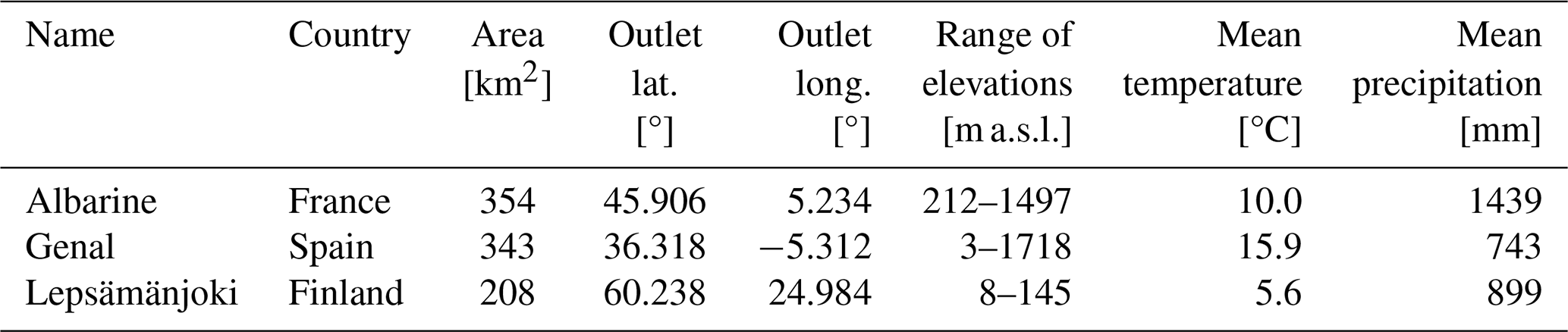
The Genal catchment, located in southern Spain, is characterised by a dry and warm climate and scarce natural vegetation. Long periods of drying are observed in the smaller reaches. The main Genal river is known to be perennial except in the downstream part of the catchment where the Genal river dries up in the summer season due to water abstraction for irrigation.
Conversely, the Lepsämänjoki catchment in Finland is characterised by a wetter and colder climate. Flow intermittence is only observed in the smallest reaches but seems to have intensified in recent years due to climate change.
The Albarine in France is characterised by a more temperate climate. Flow intermittence is particularly observed in the upstream and downstream parts of the catchment. Drying is mainly due to the seepage of the Albarine river into the soil at geological discontinuities.
2.1.2 Spatial data
Topography, soil type, land use, and hydrogeology information is needed as input to the spatially distributed hydrological model. The following data sources were used:
-
Topography. The EU-DEM v1.1 (Copernicus, 2016) with a 25 m resolution for the Albarine DRN, the Andalucía DEM (Portal Ambiental de Andalucía, https://www.juntadeandalucia.es/medioambiente/portal/landing-page-mapa/-/asset_publisher/wO880PprC6q7/content/mapa-de-elevaciones-del-terreno-de-andaluc-c3-ada-mde-/20151, last access: 15 February 2024) with a 10 m resolution for the Genal DRN, and the 10 m DEM Finland (National Land Survey of Finland, https://asiointi.maanmittauslaitos.fi/karttapaikka/tiedostopalvelu/korkeusmalli, last access: 22 March 2021) for the Lepsämänjoki DRN were employed.
-
Soil. Soil classes as well as physical parameters (field capacity, saturated water content, depth to rock) were used from the European Soil Database v2.0 (European Commission; Panagos et al., 2012). In the Genal DRN (Spain) texture and bulk density data were used from soil profiles (Llorente et al., 2018) for the calculation of parameters using pedotransfer functions (Ad-Hoc-AG, 2005; Baxter, 2007).
-
Land use. Corine Land Cover (CLC) 2012, Version 2020-20u1 Level 3 (44 classes), was used (Copernicus Land Monitoring Service 2020) to establish the land use–land cover (LULC) classes. Parameters such as albedo, crop coefficients, leaf area index (LAI), root depth, and impervious fraction area were adapted to local conditions from different sources (Allen et al., 1998; Krause, 2001; Kralisch and Krause, 2006; Neitsch et al., 2011; Faroux et al., 2013).
-
Hydrogeology. IHME1500, the International Hydrogeological Map of Europe (aquifer and lithology layers) (Duscher et al., 2015), was used to establish the classes for all DRNs.
2.1.3 Climate data
The ERA5-Land reanalysis (Muñoz-Sabater et al., 2021) was used to as climate forcing data for the hydrological modelling. The following hourly ERA5-Land climate variables were used to compute the reference evapotranspiration using the Penman–Monteith equation (Allen et al., 1998): 2 m air temperature (°C), 2 m dew point temperature (°C), 2 m relative humidity (%), 10 m u and v wind speed components (m s−1), incoming solar radiation (W m−2), incoming thermal radiation (W m−2), and surface pressure (Pa). Hourly ERA5-Land precipitation, air temperature, and computed reference evapotranspiration were then aggregated at the daily time step to be used as climate forcing data in the hydrological model.
2.1.4 Flow state and discharge data
In order to validate the models' ability to simulate flow intermittence at the reach level, multiple data sources of flow observations were used:
-
Hydrological stations. These include discharge daily time series from gauging stations (http://leutra.geogr.uni-jena.de/DRYvER, last access: 27 November 2023). The streams are considered dry if the measured discharge is equal to 0 m3 s−1 and flowing otherwise. The ONDE network (Observatoire National des Etiages, https://onde.eaufrance.fr, last access: 6 July 2022), a French network of hydrological stations, was specifically developed to monitor intermittent rivers and gives a monthly qualitative information about the state of flow (visible flow, non-visible flow, dry).
-
Crowdsourced data from smartphone applications. These include data from DRYRivERS (https://www.dryver.eu/app, last access: 14 November 2022) and CrowdWater (https://crowdwater.ch/en/data/, last access: 20 September 2022).
-
Measurements from field campaigns for the DRYvER project. Phototraps installed along the river networks took pictures daily from 7 November 2018 to 30 April 2022 in the Albarine DRN and from 17 June to 26 September 2021 in the Lepsämänjoki DRN.
-
Observations in Google Earth images. The state of flow of the reaches was observed in the images for several dates between 2010 and 2022. The observation with Google Earth images was only possible in the Genal DRN, which has scarce vegetation.
-
Expertise of local DRYvER project partners. Some members of the DRYvER project have been studying these DRNs for several years and have a deep understanding of their hydrological behaviours. Their expertise was used to identify reaches characterised by a perennial flow. These reaches are assumed to be flowing every day during the field campaign period.
These data sources are available either as disconnected points in time and space (Fig. 2), recurrent observations at the sampling sites, or time series of daily data over periods ranging from a few months to several years.
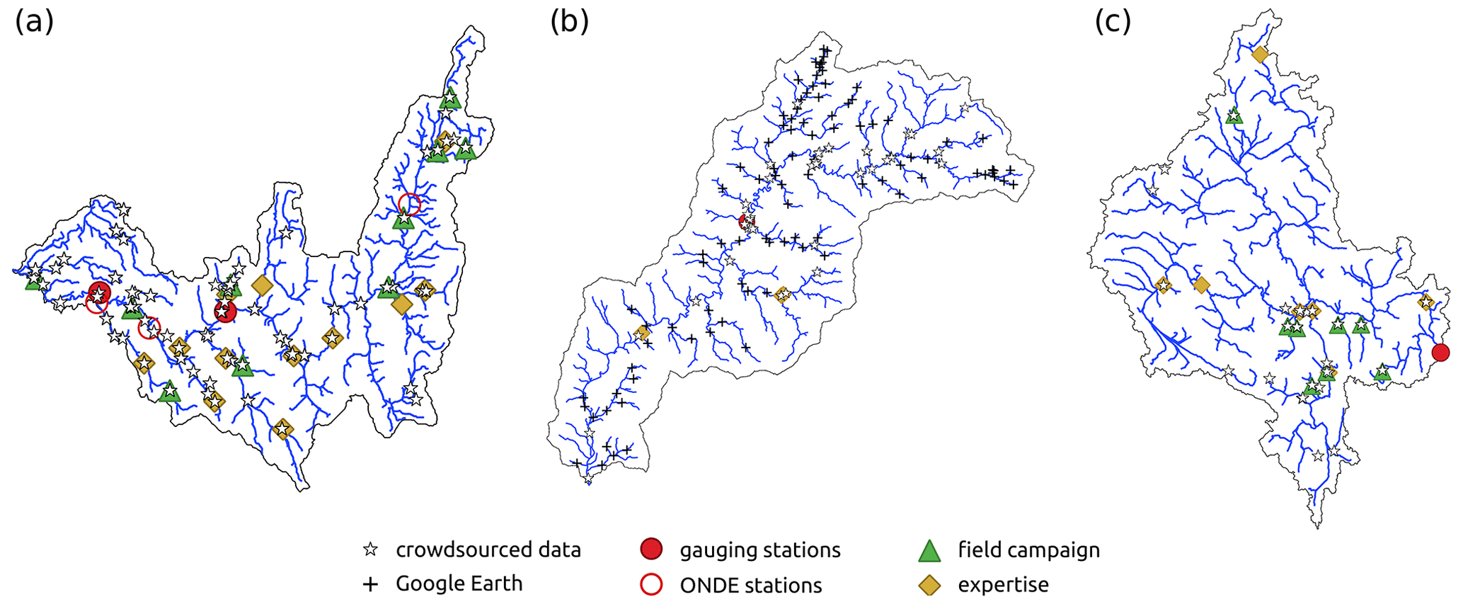
Figure 2Observed state of flow data in the (a) Albarine, (b) Genal, and (c) Lepsämänjoki DRNs.
As a result of acquiring data from multiple sources, there may be several flow state observations on the same day in the same reach. By grouping the data by reach and by date, we observe that there is simultaneity in only 0.26 % of cases on average for the three catchments (Albarine – 83 cases of simultaneity over 28 852 total cases, Genal – 16 cases over 7146, Lepsämänjoki – 12 cases over 6307). The small amount of data observed on the same day on the same reach can be explained by the complementary nature of the different sources, which each focus on different areas and periods. Of the 111 cases of simultaneity, the different sources give the same state of flow in 88 % of cases. In the case that there are several flow state observations on the same day in a reach, only one observation is kept to train the RF model. First, a filter is applied to prioritise data from direct observations (e.g. ONDE stations, crowdsourced data, phototraps, Google Earth) and remove data from indirect measurements (gauging stations). If after this selection, there are still more than one observation per reach and per day, only one observation with the predominantly observed flow state (flowing or dry) is kept.
A detailed analysis of the flow state observations and their ability to represent the drying in the river networks is presented in the Results section (Table 5 and Fig. 5).
2.2 Flow intermittence model
In order to simulate flow intermittence, a spatially distributed process-oriented hydrological model (JAMS-J2000) was implemented on the three mesoscale DRNs (detailed description of the model in Sect. 2.2.1). Once calibrated and validated, the JAMS-J2000 hydrological model enables daily streamflow time series to be simulated in each reach of the river network.
Then, the deterministic hydrological model was coupled with a stochastic model, using the model outputs and physical information to train a random forest (RF) classification model with some flow state observations. The outputs of the RF model enables the daily flow state (flowing or dry) to be predicted in each reach of the DRN, thus predicting the spatio-temporal patterns of flow intermittence.
The modelling method to simulate flow intermittence is summarised in Fig. 3 and is described in detail in the following sections.
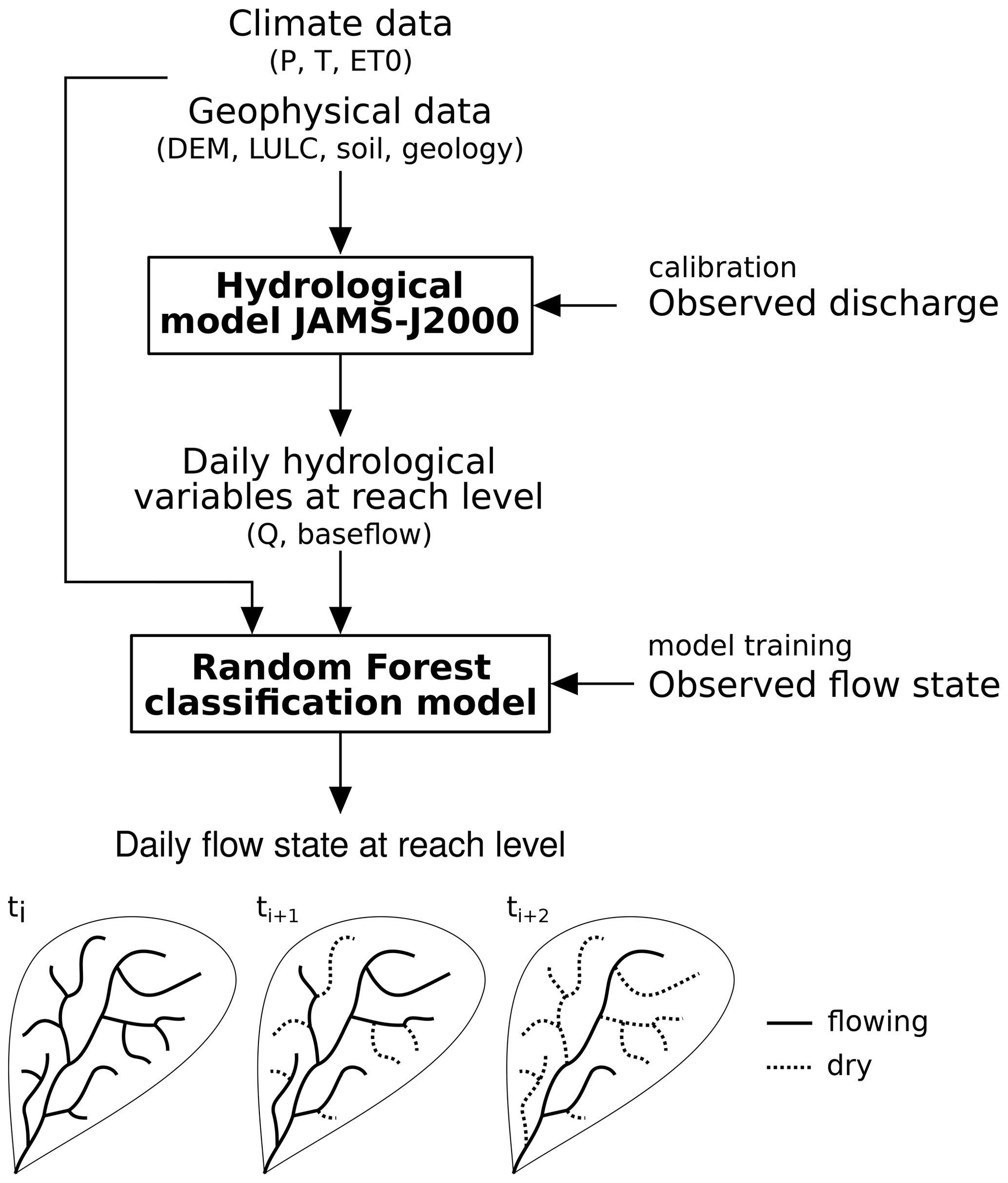
Figure 3Modelling approach to simulate flow intermittence in river networks by coupling a distributed hydrological model to a random forest classification model.
2.2.1 JAMS-J2000 hydrological model
The process-oriented JAMS-J2000 hydrological model (Kralisch and Krause, 2006) is used to simulate spatially distributed hydrological variables in the DRNs. The catchment represented in JAMS-J2000 is discretised in Hydrological Response Units (HRUs). From climate forcing data, JAMS-J2000 simulates evapotranspiration, snow processes, soil water balance, and groundwater processes at the HRU level and computes lateral flow routing to account for surface, sub-surface, and groundwater flow from hillslopes into the stream and along stream segments to the outlet of the river network (Fig. 4).
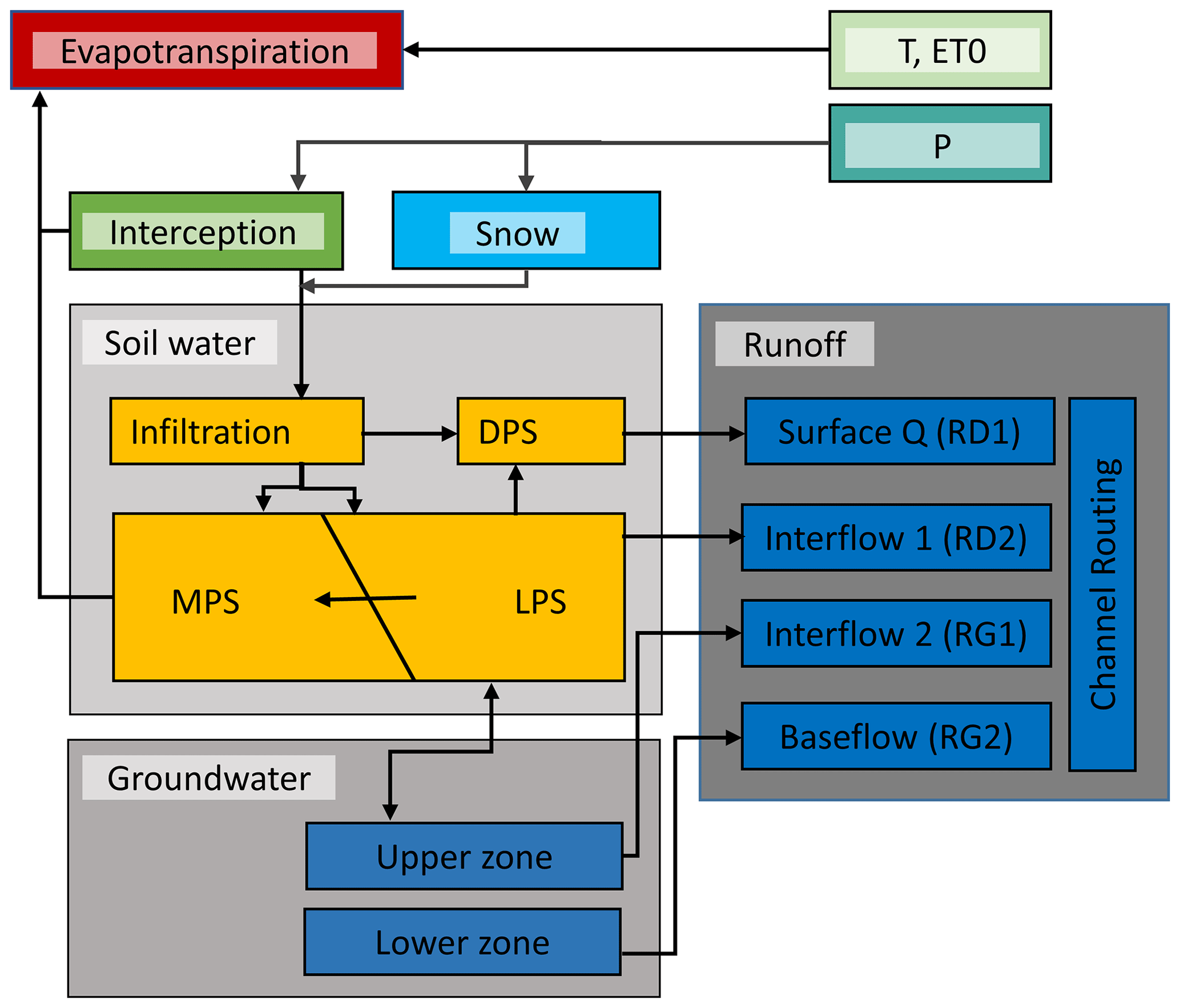
Figure 4Schematic representation of the hydrological processes modelled in JAMS-J2000 at the HRU and reach level according to Krause (2001), figure adapted from Watson et al. (2020). DPS: depression storage, MPS: middle pore storage, LPS: large pore storage.
The J2000 river networks were generated from the flow directions and flow accumulations computed from the DEMs. Observed river networks were used to validate the generated river networks and make sure that the J2000 river networks corresponds to the observed river networks (see Fig. S1–S3 in the Supplement).
Some modifications from the standard J2000 hydrological model were made for this study using the evapotranspiration module from Branger et al. (2016) to compute potential evapotranspiration using the reference evapotranspiration and spatially distributed crop coefficients. Besides, the J2000 snow module adapted by Gouttevin et al. (2017) was used.
2.2.2 Calibration of JAMS-J2000 model
This section describes only the general aspects of the method used to calibrate the JAMS-J2000 model. A full description of the calibration method as well as parameter values for each DRN is presented in Tables S1 and S2 in the Supplement.
Calibration of the JAMS-J2000 parameters was performed on larger catchments (1500 to 3700 km2) corresponding to the intermediate-scale basins studied in the DRYvER project (to bridge the gap between the DRN scale and the continental scale).
First, for the Albarine and Lepsämänjoki catchments, four lumped parameters for snow processes were calibrated to optimise the simulated snow cover area (Hall et al., 2007). Then, 15 lumped parameters and four distributed parameters were calibrated in order to optimise the simulated discharges at the gauging stations. The Kling–Gupta efficiency (KGE; Gupta et al., 2009), as well as different evaluation criteria focusing on low flows, such as the 10th percentile of the discharge, was used to assess model performance. The calibration and validation periods for the three DRNs are presented in Table 2. For the Genal catchment, the discharge data measured at the Jubrique gauging station indicated potential errors between 2004 and 2012; this period was therefore not taken into account in the calibration and validation of the model.
Table 2Calibration and validation periods. Hydrological years start on 1 October and end on 30 September.
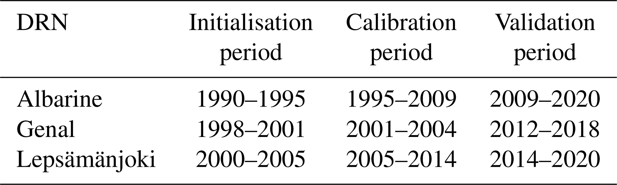
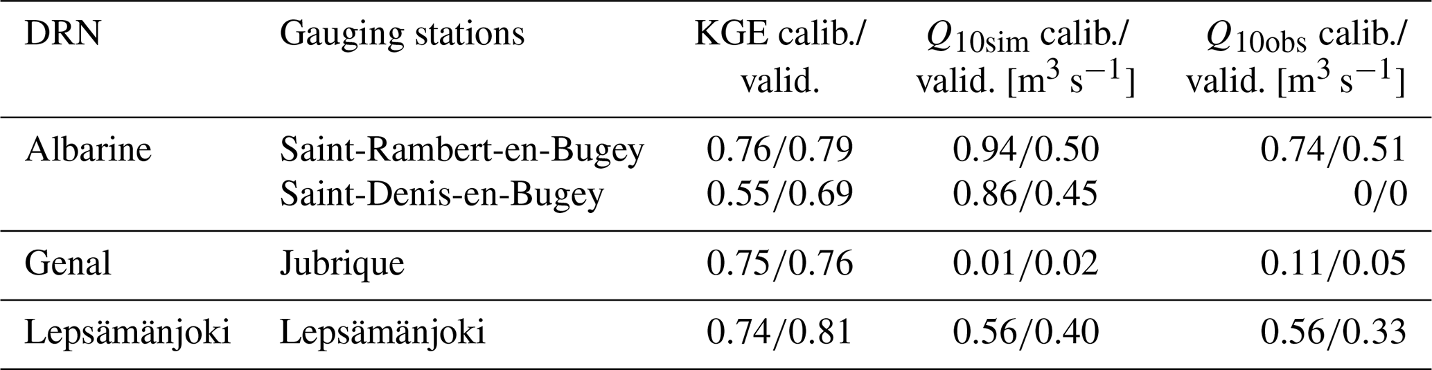
Table 3 shows the performance of the JAMS-J2000 model in simulating the discharge at the locations of the gauging stations in the three DRNs. KGE values for the calibration and validation periods show that the discharge is well simulated by the hydrological model. The comparison between the simulated and observed 10th percentile of discharge also shows that JAMS-J2000 gives good results for low flows. In the Albarine DRN, the Saint-Denis-en-Bugey station is located in the downstream part of the river, which is intermittent due to the seepage of the Albarine river in the aquifer. This explains the poorer results for this station as the seepage of the Albarine river is not represented in the JAMS-J2000 model. More details on the validation of the JAMS-J2000 model on low flows are available in the Supplement.
Table 3Validation of the JAMS-J2000 model. KGE values for the calibration and validation periods and comparison between simulated and observed 10th percentile of discharge during the calibration and validation periods.
Once calibrated, the JAMS-J2000 model is used to simulate daily hydro-meteorological variables such as spatially distributed discharge and groundwater contribution, as well as evapotranspiration, snowmelt, soil saturation and groundwater saturation at the catchment scale from 1 October 2005 to 30 April 2022 in the three DRNs.
2.2.3 Random forest classification model
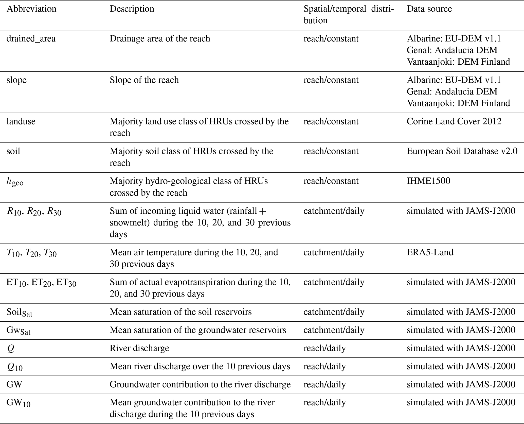
Results of the JAMS-J2000 hydrological models are used as input data to a machine learning model to predict the flow intermittence at the reach level. The random forest (RF) classification and regression model (Breiman, 2001) is used to predict the daily state of flow (dry or flowing) at the reach level. The RF model uses 20 covariates based on Beaufort et al. (2019) (Table 4):
-
reach physical characteristics, including drainage area, slope, type of land use, type of soil, and hydrogeological class around the reaches;
-
daily hydro-meteorological variables aggregated at the catchment scale, including incoming liquid water, temperature, and actual evapotranspiration during the 10, 20 and 30 previous days, as well as soil and groundwater saturation;
-
spatially distributed hydrological variables simulated with JAMS-J2000, including discharge and groundwater contribution (at t0 and averaged over the 10 previous days).
Table 4List of the covariates used in the RF model to predict the spatially distributed daily state of flow.
The RF models were implemented and calculated using the R package “ranger” (Wright et al., 2020).
For each DRN, the RF models are trained using flow state observations and then used to extrapolate the daily state of flow in each reach during the simulation period (1 October 2005–30 April 2022) spatially and temporally. To use most of the observed flow state data (Sect. 2.1.4), the RF model is trained with all available data.
During the training phase of a RF model, a subset of variables is randomly selected at the node's splitting point in each random forest tree (Breiman, 2001). In this study, the RF is trained 20 times in order to take this structural uncertainty into account.
The ability of the RF model to represent flow intermittence is evaluated with four efficiency criteria: sensitivity (SEN; probability of correctly detecting drying events), specificity (SPE; probability of correctly detecting flowing events), accuracy (ACC; probability of correctly simulating the flow condition), and false alarm ratio (FAR; probability of wrongly predicting a drying event). These criteria are calculated as follows:
with a the number of dry observations correctly simulated by the model, b the number of flowing observations that were simulated as dry, c the number of dry observations that were simulated as flowing, and d the number of flowing observations correctly simulated by the model.
2.3 Sensitivity analysis of the RF model
2.3.1 Sensitivity to the size of the training sample
First, the sensitivity of the RF model to the size of the training sample is tested by randomly selecting 75 % of the flow state observations to train the RF model for each of the 20 runs. The RF model is then evaluated on the remaining 25 %. For the 20 runs, the selection of the 75 % of training data is based on a different random draw. This first test aims at evaluating the impact of using a reduced training dataset on the prediction of flow intermittence. It also aims at evaluating the error of the RF model on a validation sample.
2.3.2 Sensitivity to the type of flow state observed data
As presented in Sect. 2.1.4, the collected flow state observation datasets used to train the RF model are heterogeneous in terms of spatial and temporal distributions of the observations and representativity of different types of flow regimes. The sensitivity of the RF model to each type of observed data (stations, field campaign, crowdsourced data, Google Earth, expertise) is evaluated by removing each type of data from the training dataset in turn and then comparing the RF performance and the predicted flow intermittence patterns. The RF performance is evaluated on the whole dataset of flow state observations in order to compare the performance on the same validation dataset. The objective of this analysis is to assess the amount of useful information contributed by each type of data.
2.3.3 Sensitivity to the geology data
The last test aims at analysing the sensitivity of the RF model to different degrees of accuracy of covariates. Here, we focus on the study case of the Albarine DRN, in which a main cause of intermittence is the infiltration of the riverbed in moraine deposits and karstic soils.
The European IHME1500 map used to define the geological classes in the hydrological model (JAMS-J2000 + RF), with a scale of 1:1 500 000, shows three classes of geology in the Albarine catchment (karst, fine sediments, and coarse sediments). On the other hand, the French BD Charm-50 map (BRGM, 2020), with a scale of 1:50 000, shows 71 different geological classes.
The RF is trained with the geological classes from the BD Charm-50 map to evaluate the impact of the precision of geological data in a catchment where flow intermittence is very influenced by the geological context. In this test, the JAMS-J2000 is still parameterised based on the IHME1500 map; only the input geology classes of the RF are modified.
3.1 Observed flow state data analysis
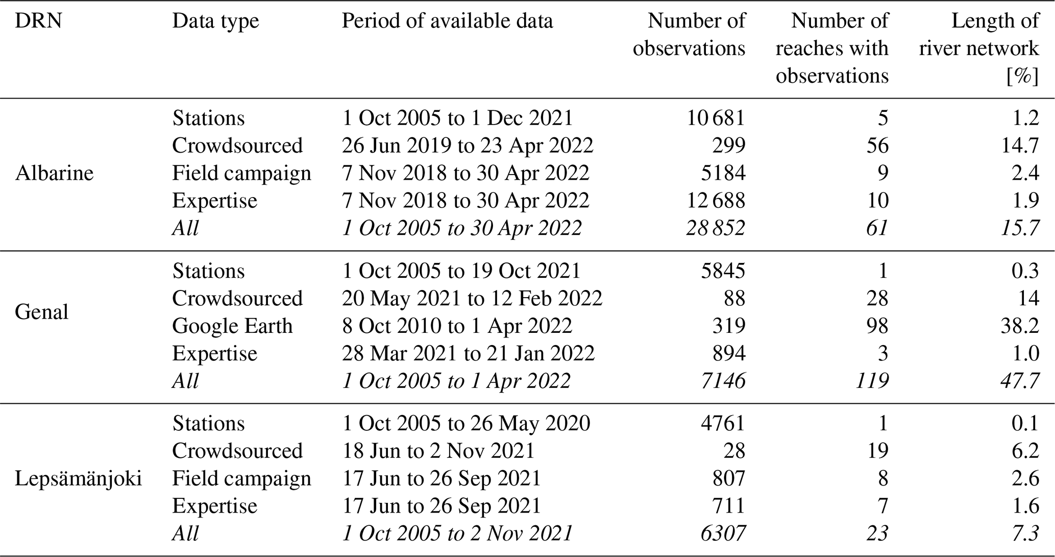
Table 5 shows general statistics on the distribution of the observed flow state between the different datasets and the coverage of the river networks. The gauging stations are the main source of observed data in terms of number of observations. They give information on long time periods with a regular time step, but the number of stations in the DRN is limited (one station in the Genal and Lepsämänjoki DRNs and five stations in the Albarine DRN), which means that stations cannot provide useful information about the spatial patterns of drying in the DRNs. The field campaigns (with expertise) are the second source of observed data. They cover a shorter time period than the stations (3 months in Lepsämänjoki and 3.5 years in the Albarine) but have a better spatial coverage of the river network than the stations. In the Genal DRN, observed data from Google Earth images show a very good spatial coverage with about 38 % of the river network, with at least one observation along the period of available data. It also covers a long time period (11.5 years) but with only a few observations per reach (between one and eight observations per reach). Crowdsourced data only represent a very small fraction (0.6 % to 2.8 %) but have a good spatial coverage, with around 14 % of the Albarine and Genal river networks covered.
Table 5Flow observations in the studied DRNs (from 1 October 2005 to 30 April 2022). The use of italics denotes the distinction between the four distinct types of data (stations, crowdsourced, field campaign, expertise) and all the data grouped together (all).
Observed data have different distributions in time and space in the DRNs (Fig. 5). For the three DRNs, there are observed data on the different classes of reaches (classified according to their drainage area), but there are more data available in the class of reaches with the largest drainage area. This is due to the data from gauging stations that are located along the main river and which represent the largest share of the data. The Albarine basin is the only one to have a full seasonal coverage on the different types of reaches. Reaches with small drainage areas in the Genal and Lepsämänjoki DRNs have mainly observed data between June and September and have missing data during the other months of the year (especially December and January). This shows that the collection of observed data on flow intermittence tends to be focused on the dry season and that there is almost no information on the state of flow for small river sections during winter.
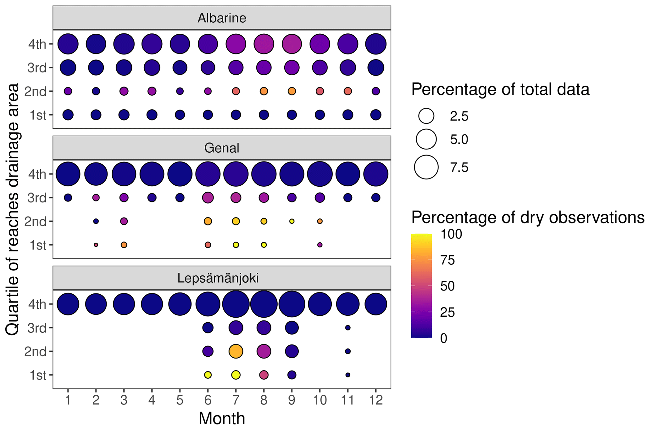
Figure 5Distribution in space and time of flow state data. The size of the dots indicates the percentage of total available data per month and per class of drainage area and the colour the percentage of dry observations per month and class of drainage area.
Figure 5 also shows a seasonal distribution of the no-flow observations along the river networks. There is a clear spatio-temporal distribution of the no-flow observations in Lepsämänjoki DRN, with most of the drying events occurring in June and July in reaches with the smallest drainage area. Drying events gradually decrease with the size of the reaches drainage area, and the main river is perennial. However, drying events seem to be over-represented during the summer season because in the smallest reaches, 100 % of the observations are dry, whereas it is known that in this catchment, not all small reaches dry up, and they do not dry for more than a few weeks. In the Genal DRN, the peak of the drying season seems to be between June and September, but drying events are also observed in early spring and autumn. Most of the dry events are observed in the small reaches, but a few dry events are also observed in the downstream part of the Genal river due to water abstraction of irrigation (around 4 % of the observations in June and July). Drying events are observed later in the season – from August to October – in the Albarine DRN and are localised in small reaches but also in the main river due to the seepage of the Albarine river into the soil (around 30 % of dry observations in the Albarine between July and August). The smallest reaches (with a drainage area lower than the 25th percentile) only show flowing observation, which shows that no-flow observations may be lacking in these reaches.
3.2 Prediction of flow intermittence
This section presents the results of the simulation of flow intermittence with the JAMS-J2000 + RF modelling.
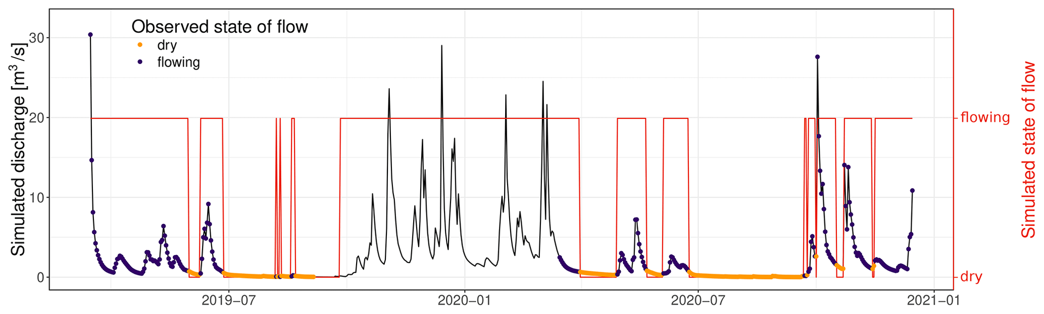
Figure 6Daily state of flow predicted by the RF model (red) in the reach 2 443 600 in the Albarine DRN compared to the discharge simulated by the JAMS-J2000 model (black) and the observed state of flow collected from a phototrap (orange – dry, purple – flowing).
Figure 6 shows an example of the state of flow prediction in one reach of the Albarine DRN. Comparison of the observed state of flow and the discharge simulated with the JAMS-J2000 model shows that the hydrological model alone is not sufficient to reproduce the periods with no flow. The transition from a flowing to a dry state cannot be easily inferred from the simulated flows alone since there are periods when the simulated discharge is relatively high (e.g. in late 2020) while the phototrap indicates a dry state, whereas on other periods, the simulated discharge is low while the phototrap indicates a flowing state (e.g. late summer 2019). However, the flow state predicted by the RF model is in good agreement with the observed flow states, which shows the usefulness of the coupling between the spatialised hydrological JAMS-J2000 model and the RF model.
To enhance the precision of evaluating the coupled JAMS-J2000 + RF model to represent flow intermittence across the entire river systems, the model underwent training and testing using two distinct configurations: configuration 0 involved training the RF model with 100 % of the observed data, while configuration 1 involved training the RF model with 75 % of the observed data and validating its performance on the remaining 25 %. The SEN, SPE, ACC, and FAR values obtained with the reduced training sample (configuration 1) are indicators of the RF model error to extrapolate the prediction of the state of flow on reaches and dates that are not represented in the training dataset. With configuration 0, the model perfectly reproduces the observed drying and flowing events in the three DRNs (SEN and SPE = 1), whereas the performance of the RF model is decreased with configuration 1 (Fig. 7). The Albarine and Lepsämänjoki DRNs only show a slight decrease in the performance: the model still correctly predicts more than 90 % of the no-flow observations and has a FAR around 5 %. The Genal DRN is more impacted by the removal of some of the observed data; the mean SEN drops to 65 %, and the mean FAR is 19 %. Specificity is above 0.99 for the three catchments, which means that the RF model predicts flowing events almost perfectly with configuration 1. ACC is also very close to 1 (>0.98); this is due to the fact that flowing events are much more represented than drying events in the observed dataset, so prediction errors for dry events are negligible compared with the near-perfect predictions of flowing events.
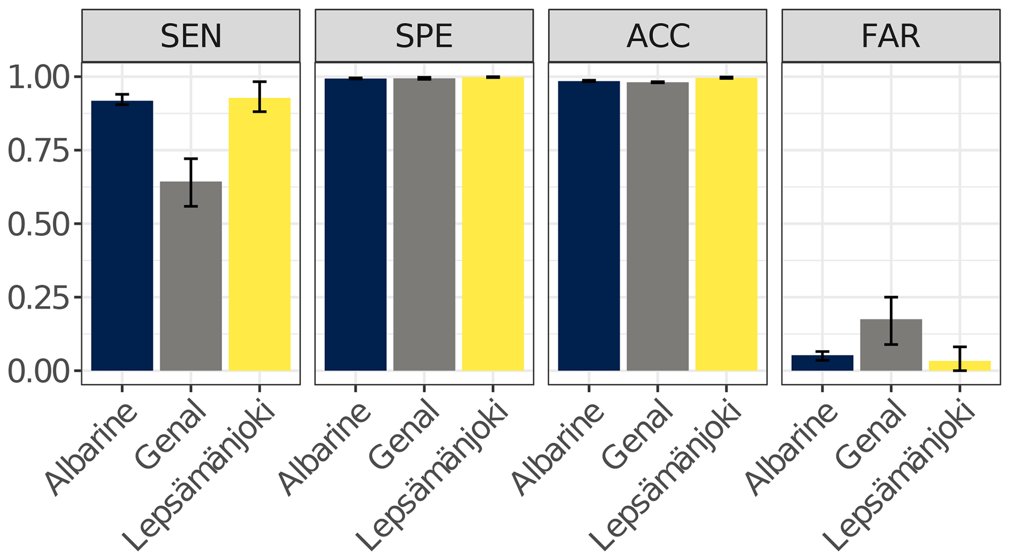
Figure 7Performance of the RF model when the model is trained with 75 % of observed data and tested on the remaining 25 % (configuration 1). Bars show the mean value, and error bars show the range of values of the ensemble of the 20 runs of the RF model with configuration 1. SEN: sensitivity. SPE: specificity. ACC: accuracy. FAR: false alarm ratio.
These results show that there is a high confidence of the prediction in the general dynamics of drying in the Albarine and Lepsämänjoki DRNs but higher uncertainty for the Genal DRN (see discussion in Sect. 4.2).
The next sections firstly present flow intermittence modelling results obtained with configuration 0 in Sect. 3.3 and 3.4 and secondly the uncertainty related to the input data (size of the training sample with configuration 1, type of flow state observed data, and geology data) in Sect. 3.5.
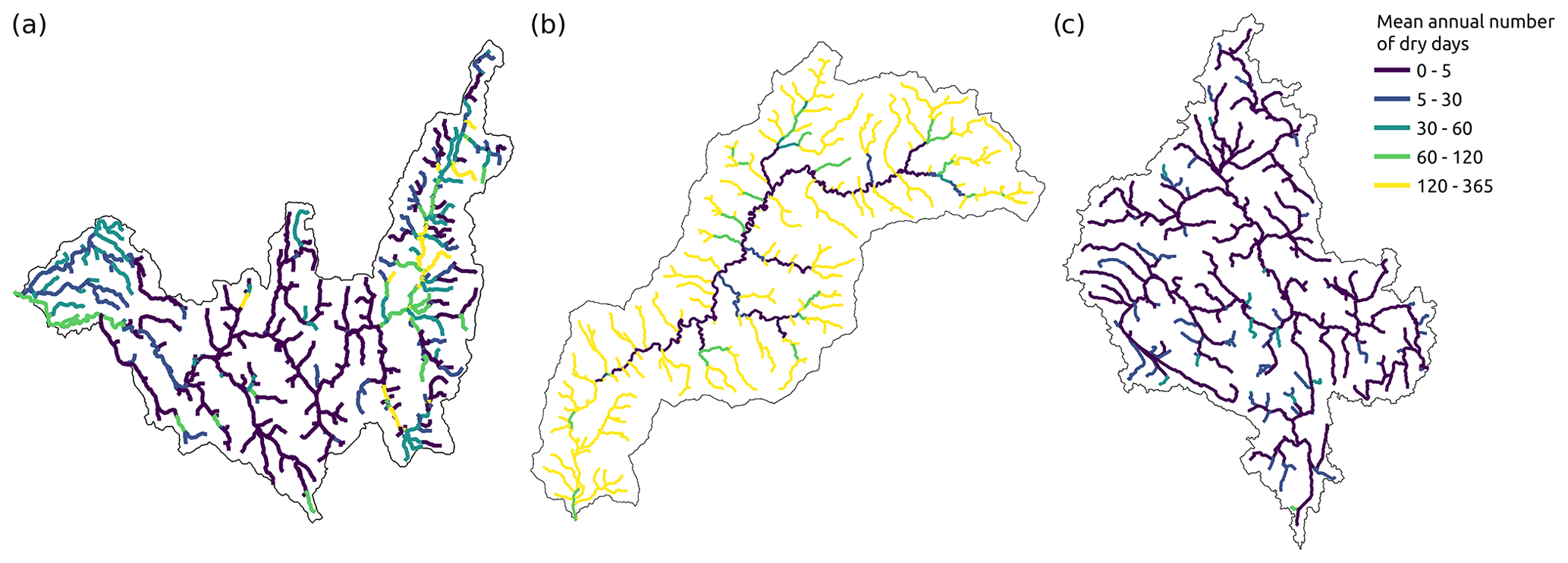
Figure 8Predicted average annual number of dry days for each reach of the (a) Albarine, (b) Genal, and (c) Lepsämänjoki DRNs.
3.3 Simulated spatial and seasonal patterns of flow intermittence
Regarding the spatial pattern of flow intermittence, the model simulates more drying in the small tributaries for the three DRNs (Fig. 8). For the Albarine and Genal DRNs, the flow intermittence of the main river in the downstream part of the catchment, due to seepage for the Albarine and water abstraction for irrigation in Genal, is well reproduced by the model. Simulated spatial patterns of drying have been validated by local experts, who confirmed that they are consistent with their observations (Figs. S13 and S14).
Figure 9 shows the mean interannual variations of the fraction of the dry river network through the year. It shows that the drying is limited to the end of May until the end of August in the Lepsämänjoki DRN, and then the mean annual maximum of drying usually does not exceed 9 % of the river network. In the Albarine DRN, the mean annual maximum of drying occurs in early September with between 24 % and 27 % of the dry river network. More than 10 % of the river network is continuously dry between July and the end of September. The model predicts some flow intermittence throughout the year (between 1 % and 4 % of the dry river network during the winter season). In the Genal DRN, the river network can dry up to 78 %–80 % in August, and more than 50% of the river network is dry from June to mid-September. The fraction of dry river network in Genal during the winter season stays relatively high (between 6 % and 26 %), but the lack of observed data over this period makes the results particularly uncertain.
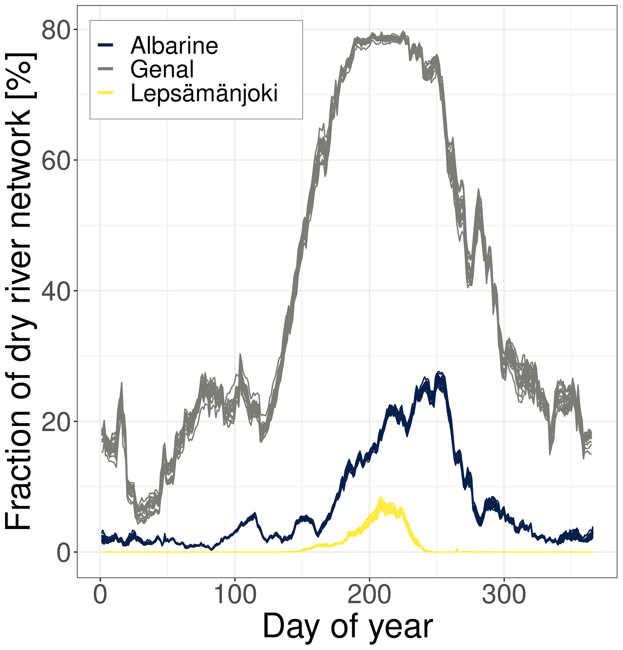
Figure 9Seasonal variability of the fraction river network that gets dry (inter-annual average of the percentage of total number of kilometres of rivers). For each DRN, the lines represent the ensemble of the 20 runs of the RF model.
Overall, the model successfully represents the general spatio-temporal patterns of drying in the three contrasted European DRNs, with intense and long periods of drying in the Genal catchment, characterised by a dry and warm climate; regular and localised drying up due to the geological context in the Albarine catchment; and short and limited in space drying in the Lepsämänjoki catchment, characterised by a more humid climate but that is mild in summer.
3.4 Analysis of the covariates
The ranking of the most important covariates in the RF models reflects the different contexts of flow intermittence in the DRNs. In the DRNs with more complex spatial patterns of drying, the RF gives more weight to the variables describing the reach characteristics. For all three DRNs, the drainage area of the reaches and their slopes are the two most important variables for the prediction of the flow state (Fig. 10).
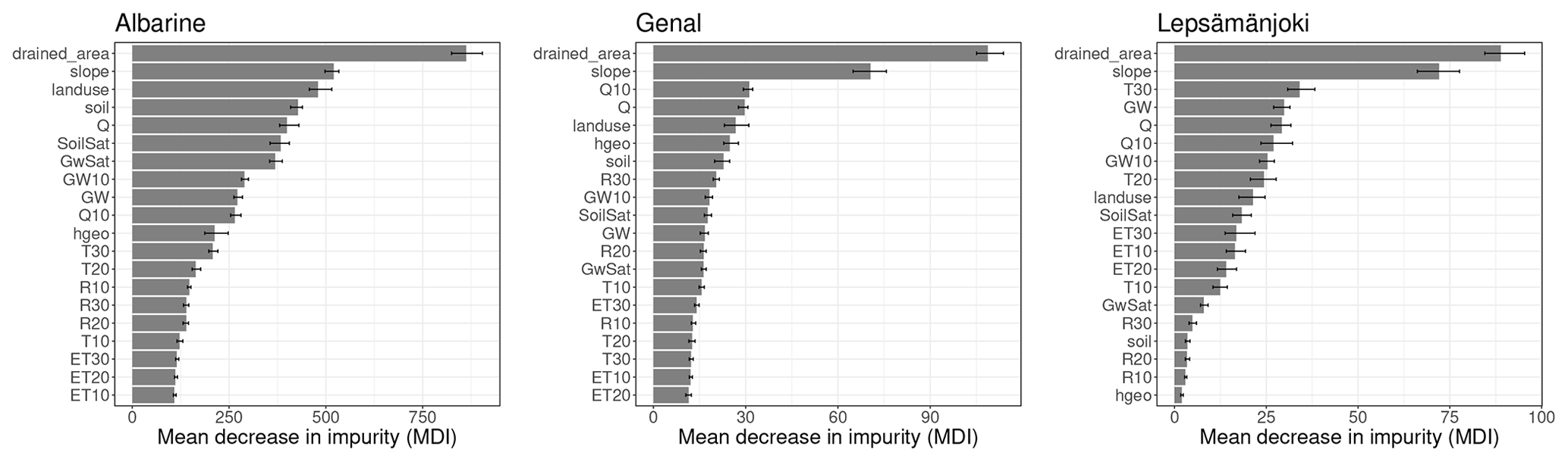
Figure 10Importance of the covariates in the RF models (mean decrease in impurity (Archer and Kimes, 2008)) for the three DRNs. Bars represent the mean decrease in impurity (MDI) and the error bars the minimum and maximum values of MDI for the 20 runs of the RF model.
For the Lepsämänjoki DRN, the next most important variables are the mean catchment air temperature during the previous 30 d (T30), the simulated discharge, and simulated groundwater contribution to the discharge (GW10 and GW). These three variables give information on the hydro-meteorological situation in the catchment and define the temporal variability of drying. T30 allows seasonal variability to be captured and makes a distinction between winter low flows, when precipitation is stored as snow in the basin, and summer low flows, when drying is observed in small streams.
For the Genal DRN, the third and fourth most important covariates are the mean discharge during the 10 previous days and the current discharge, which shows that the temporal dynamics of drying is mainly controlled by the simulated discharge in the reaches. The fifth most important variable is the land use, which reflects the more concentrated agricultural areas, with a water demand for irrigation, in the downstream part of the basin.
In the Albarine DRN, the most important variables, after the reaches drainage area and slope, are the land use and soil types around the reaches and the current discharge. The four most important variables do not reflect the main cause of drying in the Albarine, which is the seepage of the river in moraine deposit areas. The classes of geology causing flow intermittence in the Albarine are not represented in the IHME1500 dataset, which may explains why other spatial characteristics are used in the RF model to reproduce the spatial pattern of drying.
3.5 Sensitivity to the input data
3.5.1 Sensitivity to the size of the training sample
Figure 11 shows the impact of the size of the training sample on the simulated seasonal pattern of drying in the DRNs. The RF model is either trained with 100 % of available observed data (configuration 0), or 75 % of the observed data (configuration 1). For the Lepsämänjoki DRN there is no visible impact of reducing the training dataset on the predicted flow intermittence. In the Albarine and Genal DRNs, the results show that the uncertainty increases particularly during the winter season, when there are fewer observations.
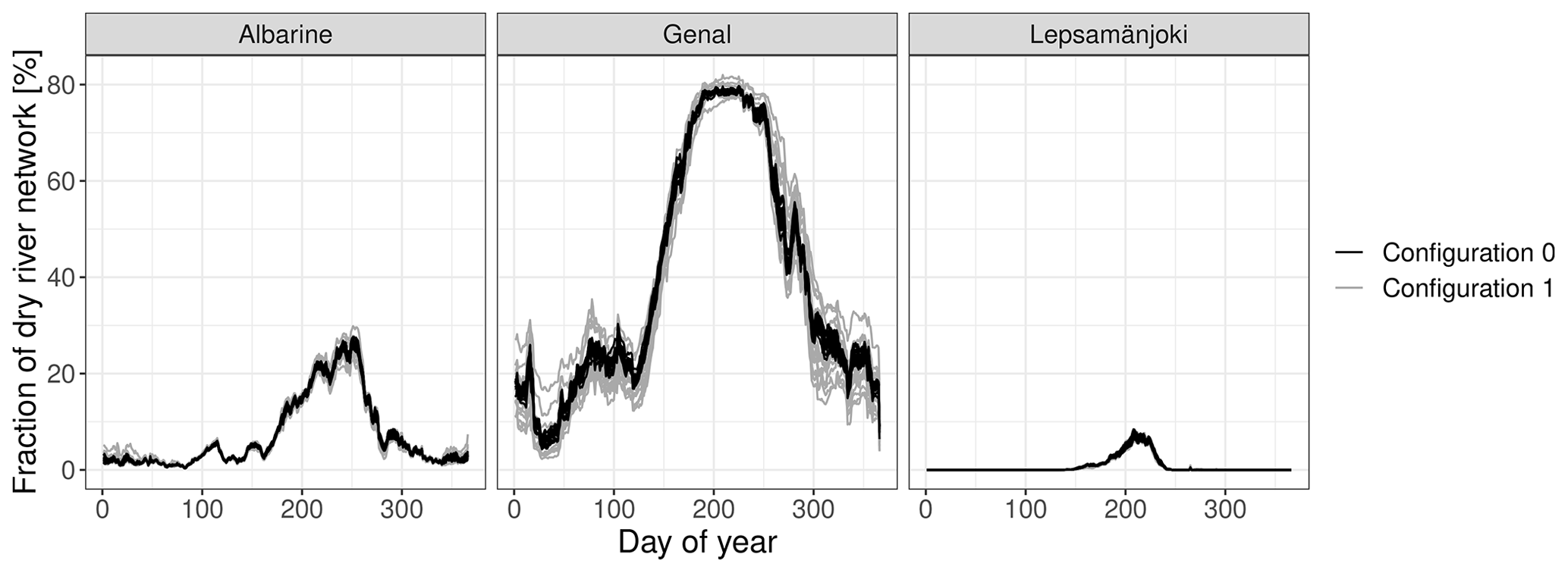
Figure 11Sensitivity of the simulated length of the dry river network to the size of the raining sample. Configuration 0 (black): the RF model is trained with 100 % of the observed data. Configuration 1 (grey): the RF model is trained with 75 % of the observed data.
These results show that the RF model is more sensitive to the representativity of drying in the observed data recorded than in the amount of data itself. The Lepsämänjoki DRN has fewer observations and a poorer spatial and temporal coverage of the observed data than the Genal DRN, but the model is more robust in Lepsämänjoki than in Genal. The higher sensitivity of the Genal DRN to the training dataset can be explained by the fact that the DRN is more affected by drying; a very large part of the river network dries every year and during long periods (several weeks to several months). It thus needs a larger amount of observed data to fully capture the seasonal dynamics of drying along the river network.
The importance of the covariates obtained with configuration 1 is very close to that obtained with configuration 0 (Fig. 10), which shows that for this study the importance of the covariates is not very sensitive to the size of the training sample (see Fig. S15).
3.5.2 Sensitivity to the type of flow state observed data
Figures 12 and 13 show the sensitivity of the model to the type of observed data used to train the RF. The first result is that the prediction of flow intermittence is very sensitive to the expertise data. Indeed, when this dataset is removed from the training sample, the FAR increases (43 % for Albarine, 40 % for Genal, and 7 % for Lepsämänjoki), the drying is more intense during the summer in Lepsämänjoki (maximum annual of dry fraction of the river network between 6 % and 8 % without expertise data versus 8 % to 11 % with expertise), and the drying is twice as more intense and lasts much longer in the Albarine DRN.
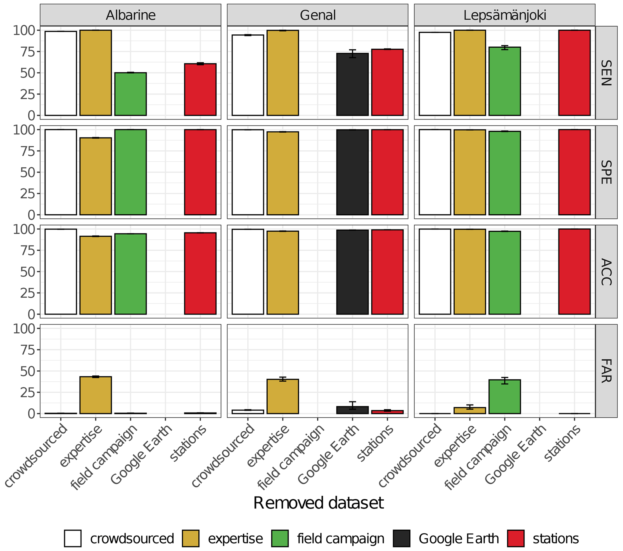
Figure 12Impact of removing a source of observed data from the training sample on the performance of the RF model.

Figure 13Impact of removing a source of observed data from the training sample on the prediction of flow intermittence.
Field campaign data also have a large impact on the prediction of flow intermittence, especially in the Albarine DRN, where the model is only able to predict 50 % of the dry days without the field data. The drying is much reduced during the summer, and there is no drying simulated from November to June. Conversely, in the Lepsämänjoki DRN, the FAR is increased without the field campaign data, and the drying is very overestimated. Expertise and field campaign data are the two most impactful datasets in Albarine and Lepsämänjoki.
In the Genal DRN, the results show that the simulated seasonal pattern of drying is very different without the Google Earth data, with a lot of drying predicted during the winter season, which can reach unrealistic values (up to 70 % of dry river network in January) (Fig. 13). In a DRN characterised by high intermittence of flows, and with few field observations, flow intermittence observations from remote sensing datasets can be very useful to better constrain the RF model.
In the Lepsämänjoki DRN, the removal of the station data from the training dataset does not impact the prediction of drying. However, in the Albarine and Genal DRNs, some of the stations are located on intermittent reaches, and their removal decreases the SEN criteria to 61 % for the Albarine and 77 % for Genal.
Crowdsourced data, which represent at most 1 % of all observations collected in the DRNs, have a visible impact on the prediction of dryness, especially during the summer. For the Albarine, the mean annual maximum of dry river network decreases from 27 % to 23 % without the crowdsourced data in early September. In the Genal DRN, the uncertainty increases without the crowdsourced data; for example, in late July–early August, the fraction of the dry river network ranges between 78 % and 80 % when the RF model is trained with all of the observed data, and it ranges between 78 % and 85 % when the crowdsourced data are removed from the training dataset. This shows that, even if they only represent a very small fraction of the observed data, crowdsourced data have a significant impact on the prediction of flow intermittence through the spatial information they provide.
3.5.3 Sensitivity to the geology data in the Albarine DRN
When the BD CHARM-50 geology map is used to define the geology classes in the covariates of the RF model, geology becomes the most important variable in the RF (versus 11th most important variable with IHME1500) (Fig. 15). The RF model also gives more weight to the mean catchment ground water and soil saturation, which shows that the physical processes causing flow intermittence in the Albarine DRN are better taken into account in the RF model when using more accurate geological data.
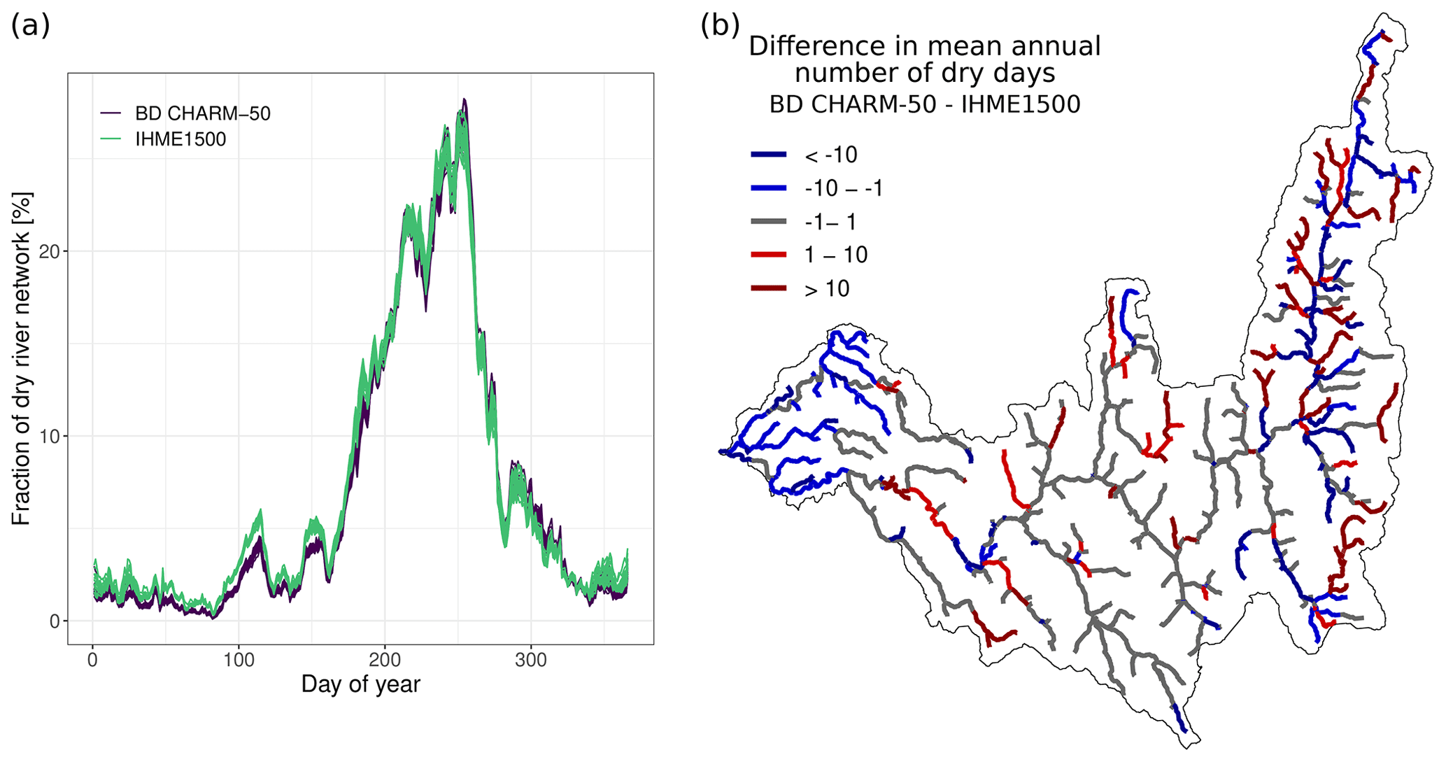
Figure 14Sensitivity of the prediction of the seasonal (a) and spatial (b) patterns of flow intermittence to geological data in the Albarine DRN. Note that in (b) values can locally largely exceed the range of [−10, 10] difference represented here.
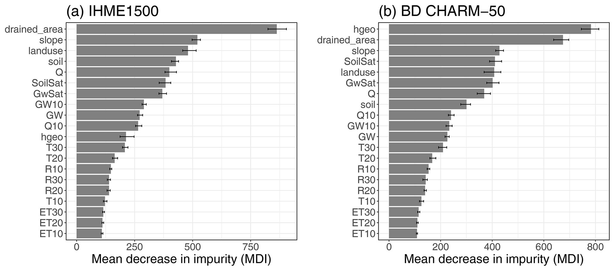
Figure 15Importance of the covariates (mean decrease in impurity (Archer and Kimes, 2008)) when the RF model is trained with the IHME (a) and the BD CHARM-50 (b) geology maps. Bars represent the mean MDI and the error bars the minimum and maximum values of MDI for the 20 runs of the RF model.
The seasonal pattern of drying is rather similar but with a bit less drying in winter and spring and a bit more drying in summer and autumn (Fig. 14a). When looking at the spatial patterns of drying, we can see some differences, especially in the upstream and downstream parts of the catchment (Fig. 14b). We presume that this is due to moraine deposits, which are represented more widely in the catchment by the BD CHARM-50 map. With the coarser geology map (IHME1500), the RF manages to predict the main spatio-temporal patterns of drying rather accurately, but the use of a more detailed geology map (BD CHARM-50) can help improve the prediction of drying at the reach scale.
4.1 Hybrid modelling to predict flow intermittence at the reach scale
The coupling between a spatially distributed model and a random forest model has a number of benefits for predicting intermittence in river systems. First, the JAMS-J2000 model represents the spatially distributed hydrological physical processes in the catchments. This enables several hydrological variables to be simulated at the HRU and the reach scale, such as evapotranspiration, soil water content, groundwater level, and discharge, which can be used as spatially distributed covariates in the RF model. Second, the JAMS-J2000 represents lateral flow routing between the HRUs and the reaches and thus represents the hydrological connectivity which cannot be represented in a RF model. However, the simulation of flow intermittence with JAMS-J2000 alone is not yet possible. The JAMS-J2000 model has difficulties in simulating periods with no flow. Even after long periods without precipitation input, the model tends to simulate residual low flows, and the reaches never completely dry up. There are also a multitude of processes causing the drying of rivers (e.g. interaction between the riverbed and the water table, seepage into karst, pumping of water from aquifers and rivers), and it is difficult to represent them all and accurately in a physical model (Fovet et al., 2021; Shanafield et al., 2021). Despite the JAMS-J2000 model's ability of simulating seepage through the alluvial riverbed (Watson et al., 2021) or water abstraction for anthropogenic uses (Branger et al., 2016), the data needed to parameterise these processes are seldom available and were not available in our case studies (e.g. daily amounts of water withdrawals and their precise locations). The use of the RF model enables flow intermittence to be simulated, even if the processes causing the drying up are not known or understood precisely beforehand since it does not require a representation of physical processes but links covariates to observed states of flow. In addition, RF models have the advantage of providing variable importance metrics (Tyralis et al., 2019) which, in our case, allow the processes leading to the drying in the DRNs to be better understood.
The question can be raised about the contribution of the RF model compared to applying a threshold on the discharge simulated by the JAMS-J2000 model below which would determine zero flows. Figure 16 shows the distributions of simulated discharges for the two types of flow conditions (flow or dry) in reach 2443600 of the Albarine (same example as in Fig. 6). For simulated discharges ranging from 0 to 4 m3 s−1, there is an intersection of the distributions for observed dry and flowing events. Setting a threshold would mean truncating the tails of these distributions. For instance, by setting a threshold to achieve a SEN of 98 % on this reach, a FAR of 26 % is obtained, as low discharges are all predicted as dry events. In contrast, with the RF model, the intersection of the distributions is well reproduced, and a FAR of 1.7 % is achieved for the same SEN (98 %). The differences in distributions between observed and simulated flow conditions can be explained by the fact that there are few “flowing” observations during winter periods with high flows in this reach. It is also challenging to extrapolate a discharge threshold value across all reaches of the network. Looking at the spatial pattern of flow intermittence in the DRNs (Fig. 8) it is clear that the threshold value should be spatially distributed to take account of local effects, but this raises the question of how this spatial distribution should be achieved.
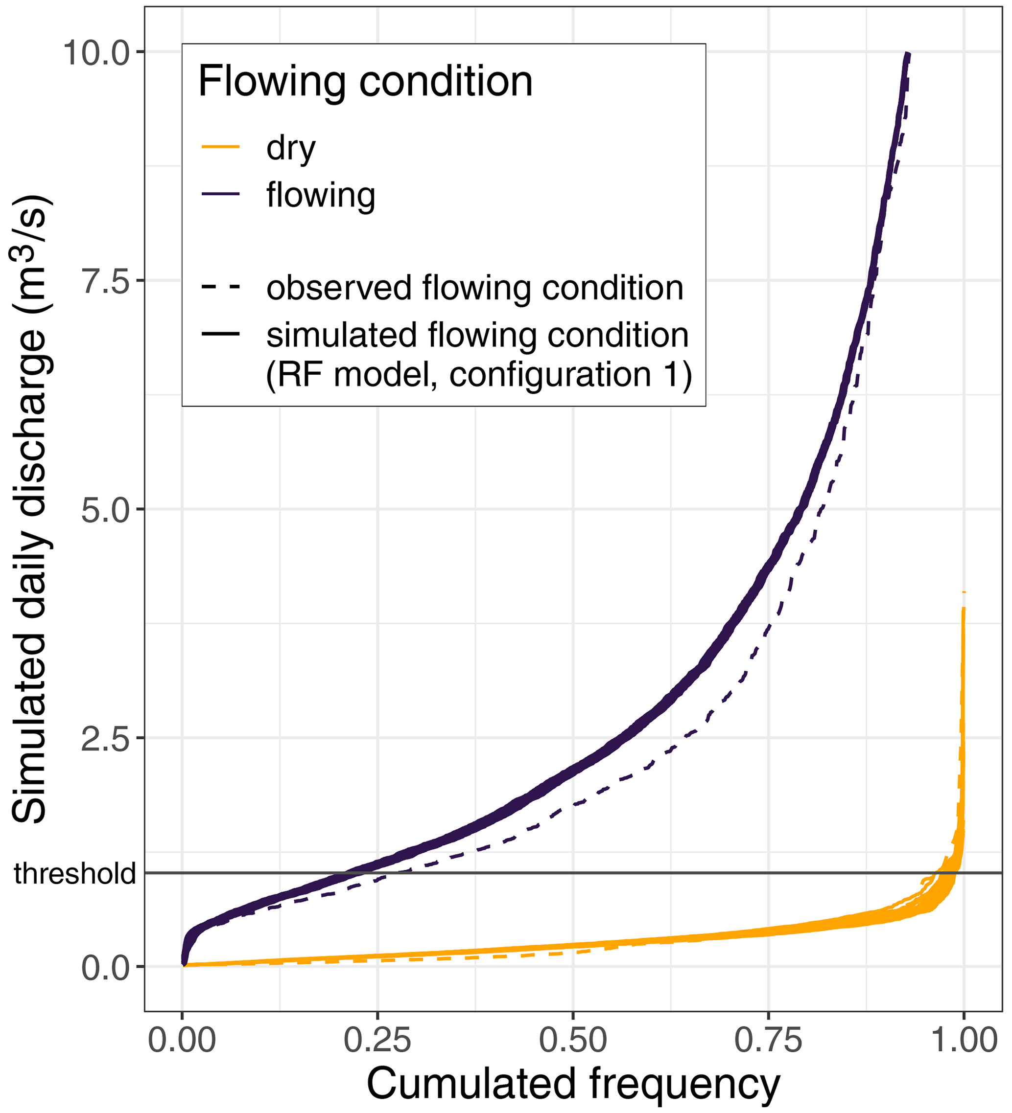
Figure 16Distribution of simulated discharge with the JAMS-J2000 model for observed and simulated (RF model 20-member ensemble with configuration 1) flowing conditions for reach 2443600 in the Albarine DRN (same reach as in Fig. 6). The horizontal black line shows an example of an applied threshold to predict flow condition from the simulated discharges (in the figure, the threshold value is set to correctly predict 98 % of the observed drying events).
The use of a spatialised hydrological model combined to a RF model is therefore very advantageous in order to be able to simulate flow states at fine time steps and in a spatialised way over the entire river network.
However, the use of a RF model has several limitations. A first limitation is that the RF model can predict the right state of flow for the wrong reasons if the causes of drying are not represented in the covariates. For the three studied DRNs, drainage area is the most important covariate, which is consistent with other studies using RF models to predict flow intermittence (Jaeger et al., 2023; González-Ferreras and Barquín, 2017; Snelder et al., 2013), but in the Albarine and Genal DRNs we know that the drying is in fact due to the geology and water abstraction, respectively. The results of the RF model do not necessarily provide a better understanding of the origin of drying in river networks if the covariates are not sufficiently precise. Most importantly, this means that a RF model trained on a specific DRN may not be robust enough to predict flow intermittence in another DRN.
One major application of this flow intermittence modelling approach is to simulate the flow states under different climate change scenarios and predict tipping points in the flow regime of the river sections, such as transitions from a perennial to an intermittent flow regime. However, the robustness of such a model for extrapolating flow intermittence in climate change projections is questionable. The RF model is trained with observed data over a relatively short period, with no observed change in the flow regime of the reaches, and it is known that RF models cannot predict events that have never been observed before (Hengl et al., 2018; Tyralis et al., 2019), which represents a major limitation for predicting the future evolution of drying spells in the DRNs. While it can be expected that the drying spells of currently intermittent reaches will be prolonged under climate change scenarios, the ability of the RF model to predict a shift from a perennial to an intermittent flow regime is not guaranteed. However, the results of this study show that the average annual number of dry days simulated for the reaches known to have perennial flow is rarely zero but can vary between 0 and 3 d yr−1. This means that in the present period, the model only simulates completely perennial flow in a few reaches. This bias in predicting the state of flow in the present period is a drawback for characterising current drying dynamics in river systems and studying the impact on biodiversity but may facilitate the prediction of drying in the context of climate projections as most of the reaches are already considered intermittent in the present period.
4.2 Observed flow state data for the modelling of flow intermittence
The results of the RF model are highly dependent on the training dataset. This study highlights the challenges of obtaining observed flow state data to train or validate the models. To accurately represent flow intermittence along river networks, the observed data ideally need to be uniformly distributed both spatially and temporally, which can be difficult to achieve.
Most studies focusing on the catchment scale collect observations from field campaigns (e.g. Llanos-Paez et al., 2023; Jaeger et al., 2023; Van Meerveld et al., 2019; Sefton et al., 2019), but such surveys generally do not allow rivers to be monitored over many years and are usually limited to portions of the river network as they can be very time-consuming.
This study shows the interest of combining different types of data with heterogeneous spatial and temporal patterns in order to maximise the information on flow condition in the river networks. This is consistent with the results of Gallart et al. (2016), who showed that combining data from citizen science and aerial photographs afforded more robust information.
The results obtained in the three basins demonstrate the need to adapt the data collection to the context of each DRN. Ideally, a large amount of homogeneously distributed data along the river network and throughout the year will introduce the least possible bias into the model, like in the Albarine DRN. However, the case of the Lepsämänjoki DRN shows that even with a small amount of data concentrated on the summer season, the predicted patterns of drying are consistent with the observations made by local experts. In contrast, with a similar amount of data, the variability of the prediction of flow intermittence in the Genal DRN is higher due to more complex spatio-temporal patterns of drying. To reduce the uncertainty in the Genal DRN, more years of observed data would be necessary, with data more evenly spread over the year to better capture the length of dry spells.
The analysis of the Albarine and Lepsämänjoki DRNs shows that data from field campaigns provide essential information on the spatial and temporal dynamics of drying, making them the most useful type of data for predicting flow intermittence in river networks. However, in the Genal DRN, where phototraps were not installed during field campaigns, remote sensing seems to be a good alternative for collecting data. Although remote sensing data can be used to detect the state of flow adequately, Gallart et al. (2016) have nevertheless pointed out several limitations: images are available at too low a frequency to study temporal patterns, and dense vegetation near the rivers may prevent the detection of the state of flow.
As shown in the results of this study, citizen science can also be a useful way of obtaining intermittence data and increasing the spatial coverage of observations. Several studies have shown the advantages of working with citizens to monitor temporary streams, especially to obtain observations in streams that would otherwise not be monitored (Turner and Richter, 2011; Buytaert et al., 2014; Gallart et al., 2016; Kampf et al., 2018). Gallart et al. (2016) and Strobl et al. (2019) studied the accuracy of data provided by citizen scientists and showed these data give an overall good indication of the hydrological state of the streams.
Expertise data indicating reaches with perennial flow proved to be crucial in reducing the over-representation of data from intermittent reaches in the RF model training data across all three DRNs. However, this raises questions about the value of such data, which is based on human perception and the error it may contain. Expert elicitation in hydrology has already shown benefits, particularly when tangible data are missing (Ye et al., 2008; Warmink et al., 2011; Sebok et al., 2016, 2022). These studies do show differences in the individual perceptions of the experts consulted, but by consulting a larger number of experts (in this study, only one or two experts were consulted per studied DRN) and by applying protocols similar to the ones proposed in these studies, the uncertainty linked to individual perception could be reduced, or at least quantified.
The general indications for data collection emerging from this study are to (1) favour a good spatial distribution of the observations by collecting data reaches with different characteristics (e.g. in terms of drainage area, geology and water abstractions), (2) collect data on intermittent sections as well as on reaches with a permanent flow regime, and (3) have time series of observations covering at least a whole year on a few points of the river network.
4.3 Delineation of the river networks
Another limitation of the study arises from the delineation of river networks. The delineation needs to be as accurate as possible to ensure that observations of flow state are assigned to the correct reaches. However, several studies such as those by Prancevic and Kirchner (2019), Van Meerveld et al. (2019), and Godsey and Kirchner (2014) have shown that river networks are dynamic systems: they extend or retract according to landscapes and climatic conditions and can also be disconnected. It is therefore difficult to delineate a fixed reference river network with a density, enabling the spatial variability of drying in the DRNs to be predicted accurately.
In this study, the density of the delineated river networks was chosen so that all observations could be assigned to a reach, but the results show that the density of the river network has an impact on the simulated patterns of drying in the DRNs. In the three studied DRNs, contradictory states of flow were observed in reaches on the same day, indicating that the density of the river networks is not high enough to capture very local processes of drying. In contrast, the density of the river network should not be too high, as it may lead to the representation of reaches with an unrealistically small drained area, for which there are no observed data available to train the RF model. This situation occurred in the Albarine DRN where the resolution of the river network had to be increased in order to capture the locations of observed data (Fig. S2), resulting in some unrealistic prediction of small perennial reaches in the upstream part of the catchment (Fig. 8).
The modelling approach, coupling a spatially distributed physical hydrological model (JAMS-J2000) with a random forest classification model, developed in this study allows the daily state of flow (dry or flowing) to be predicted at the reach scale along river networks. The results show that the models allow the main spatio-temporal patterns of drying to be successfully predicted in three contrasted European river networks.
This study also discusses the difficulty of collecting flow intermittence data to train and validate random forest models. The results show that the combination of various sources of observed flow state data is essential to form a training dataset that is representative of the actual spatio-temporal drying patterns in the drying river networks and to reduce the uncertainty of the prediction of flow intermittence.
In order to improve the modelling of flow intermittence, further improvements could be made to the models and to the collection of flow state data to train the RF model. Regarding the modelling approach, a first perspective is to add a third class of state of flow in the RF model to predict the pools' condition (i.e. stagnant water in disconnected pools) which is as important as the dry or flowing conditions for studying the ecological impact of flow intermittence (Datry et al., 2017; Bourke et al., 2023). Another perspective is to improve the parameterisation of the groundwater reservoir in the JAMS-J2000 models using observed data of groundwater level to optimise the groundwater parameters and using more precise geology data to define the geological classes in JAMS-J2000 for the DRNs where flow intermittence is influenced by geology. Regarding the collection of flow state data, one perspective is to use satellite products to collect flow intermittence data. Cavallo et al. (2022) showed that Sentinel-2 images can be used to detect flow intermittence along river networks. The use of satellite products could allow the modelling method to be transposed more easily to other river networks without the need for extensive field campaigns.
The hydrological modelling approach presented in this study will be used to project the evolution of flow intermittence in the river networks under climate change scenarios and provide flow intermittence indices to characterise the spatio-temporal dynamics of drying in the DRNs in the present and future periods. These indices will then be used to study the impact of drying on the freshwater ecosystems. One of the challenges will therefore be to analyse the hybrid model's ability to extrapolate the flow state of river sections in a future climate. In particular, it will be necessary to analyse the model's ability to simulate changes in a flow regime (for example, the transition from perennial to intermittent flow) outside its training period.
The calibrated JAMS-J2000 hydrological models for the three study catchments, the R scripts used to predict flow intermittence with a random forest algorithm, and the observed flow state data used in this study can be obtained from the corresponding author upon request.
The supplement related to this article is available online at: https://doi.org/10.5194/hess-28-851-2024-supplement.
Conceptualisation: LM, AK; model implementation and analysis: LM, AK, AD; draft preparation and discussions: LM, FB, JPV, AK. All authors read and approved the final paper.
The contact author has declared that none of the authors has any competing interests.
Publisher's note: Copernicus Publications remains neutral with regard to jurisdictional claims made in the text, published maps, institutional affiliations, or any other geographical representation in this paper. While Copernicus Publications makes every effort to include appropriate place names, the final responsibility lies with the authors.
We thank Thibault Datry and Bertrand Launay (INRAE RiverLy) for their expertise on the Albarine DRN; Heikki Mykrä and Henna Snåre (SYKE) for their expertise on the Lepsämänjoki DRN; and Nuria Bonada, Maria Soria (University of Barcelona), Amaia Angula Rodeles (Universidad de Cantabria), and Nuria Cid (INRAE) for their expertise on the Genal DRN. We also thank all the other members of DRN teams of the DRYvER project for sharing local data and collecting flow intermittence observations in the DRNs.
This research has been supported by the European Union's Horizon 2020 Research and Innovation programme through the DRYvER project (Securing Biodiversity, Functional Integrity and Ecosystem Services in Drying River Networks, award number 869226).
This paper was edited by Fabrizio Fenicia and reviewed by three anonymous referees.
Acuña, V., Datry, T., Marshall, J., Barceló, D., Dahm, C. N., Ginebreda, A., McGregor, G., Sabater, S., Tockner, K., and Palmer, M.: Why should we care about temporary waterways?, Science, 343, 1080–1081, https://doi.org/10.1126/science.1246666, 2014. a
Ad-Hoc-AG: Bodenkundliche Kartieranleitungmit 41 Abbildungen, 103 Tabellen und 31 Listen, Bundesanst. für Geowiss. und Rohstoffe, Hannover, ISBN 978-3-510-95920-4, http://slubdd.de/katalog?TN_libero_mab2 (last access: 24 August 2022), 2005. a
Allen, R. G., Pereira, L. S., Raes, D., and Smith, M.: Crop evapotranspiration-Guidelines for computing crop water requirements-FAO Irrigation and drainage paper 56, Fao, Rome, http://www.fao.org/docrep/x0490e/x0490e00.htm (last access: 13 September 2022), 1998. a, b
Archer, K. J. and Kimes, R. V.: Empirical characterization of random forest variable importance measures, Comput. Stat. Data Anal., 52, 2249–2260, https://doi.org/10.1016/j.csda.2007.08.015, 2008. a, b
Baxter, S.: Guidelines for soil description, Experimental Agriculture, 43, Food and Agriculture Organization of the United Nations, Rome, 263–264, https://doi.org/10.1017/S0014479706384906, 2007. a
Beaufort, A., Carreau, J., and Sauquet, E.: A classification approach to reconstruct local daily drying dynamics at headwater streams, Hydrol. Process., 33, 1896–1912, https://doi.org/10.1002/hyp.13445, 2019. a, b, c, d
Belemtougri, P. A.: Compréhension et caractérisation de l'intermittence du réseau hydrographique en Afrique: développements méthodologiques et applications hydrologiques, PhD thesis, Sorbonne université, Sorbonne, https://cnrs.hal.science/tel-03900431/ (last access: 3 January 2023), 2022. a, b
Bond, N. R., Lake, P. S., and Arthington, A. H.: The impacts of drought on freshwater ecosystems: an Australian perspective, Hydrobiologia, 600, 3–16, https://doi.org/10.1007/s10750-008-9326-z, 2008. a
Bourke, S. A., Shanafield, M., Hedley, P., Chapman, S., and Dogramaci, S.: A hydrological framework for persistent pools along non-perennial rivers, Hydrol. Earth Syst. Sci., 27, 809–836, https://doi.org/10.5194/hess-27-809-2023, 2023. a
Branger, F., Gouttevin, I., Tilmant, F., Cipriani, T., Barachet, C., Montginoul, M., Le Gros, C., Sauquet, E., Braud, I., and Leblois, E.: Modélisation hydrologique distribuée du Rhône, Tech. rep., Irstea, https://hal.science/hal-02605058/ (last access: 15 February 2024), 2016. a, b
Breiman, L.: Random forests, Mach. Learn., 45, 5–32, https://doi.org/10.1023/a:1010933404324, 2001. a, b
BRGM: Bureau de Recherches Géologiques et Minières, BD Charm-50, infoTerre, http://infoterre.brgm.fr/formulaire/telechargement-cartes-geologiques-departementales-150-000-bd (last access: 26 January 2023), 2020. a
Buttle, J. M., Boon, S., Peters, D., Spence, C., Van Meerveld, H., and Whitfield, P.: An overview of temporary stream hydrology in Canada, Can. Water Resour. J./Revue Canadienne Des Ressources Hydriques, 37, 279–310, 2012. a
Buytaert,W., Zulkafli, Z., Grainger, S., Acosta, L., Alemie, T. C., Bastiaensen, J., De Bièvre, B., Bhusal, J., Clark, J., Dewulf, A., Foggin, M., Hannah, D. M., Hergarten, C., Isaeva, A., Karpouzoglou, T., Pandeya, B., Paudel, D., Sharma, K., Steenhuis, T., Tilahun, S., Van Hecken, G., and Zhumanova, M.: Citizen science in hydrology and water resources: opportunities for knowledge generation, ecosystem service management, and sustainable development, Front. Earth Sci., 2, 26, https://doi.org/10.3389/feart.2014.00026, 2014. a
Cavallo, C., Papa, M. N., Negro, G., Gargiulo, M., Ruello, G., and Vezza, P.: Exploiting Sentinel-2 dataset to assess flow intermittency in non-perennial rivers, Sci. Rep., 12, 1–16, https://doi.org/10.1038/s41598-022-26034-z, 2022. a
Copernicus: European Digital Elevation Model (EU-DEM), version 1.1, https://land.copernicus.eu/imagery-in-situ/eu-dem/eu-dem-v1 (last access: 22 March 2021), 2016. a
Daliakopoulos, I. N. and Tsanis, I. K.: Comparison of an artificial neural network and a conceptual rainfall–runoff model in the simulation of ephemeral streamflow, Hydrolog. Sci. J., 61, 2763–2774, https://doi.org/10.1080/02626667.2016.1154151, 2016. a
Datry, T., Larned, S. T., and Tockner, K.: Intermittent rivers: a challenge for freshwater ecology, BioScience, 64, 229–235, 2014. a
Datry, T., Pella, H., Leigh, C., Bonada, N., and Hugueny, B.: A landscape approach to advance intermittent river ecology, Freshwater Biol., 61, 1200–1213, https://doi.org/10.1093/biosci/bit027, 2016. a
Datry, T., Boulton, A. J., Bonada, N., Fritz, K., Leigh, C., Sauquet, E., Tockner, K., Hugueny, B., and Dahm, C. N.: Flow intermittence and ecosystem services in rivers of the Anthropocene, J. Appl. Ecol., 55, 353–364, https://doi.org/10.1111/1365-2664.12941, 2017. a
Datry, T., Allen, D., Argelich, R., Barquin, J., Bonada, N., Boulton, A., Branger, F., Cai, Y., Cañedo-Argüelles, M., Cid, N., Csabai, Z., Dallimer, M., de Araújo, J. C., Declerck, S., Dekker, T., Döll, P., Encalada, A., Forcellini, M., Foulquier, A., Heino, J., Jabot, F., Keszler, P., Kopperoinen, L., Kralisch, S., Künne, A., Lamouroux, N., Lauvernet, C., Lehtoranta, V., Loskotová, B., Marcé, R., Martin Ortega, J., Matauschek, C., Miliša, M., Mogyorósi, S., Moya, N., Müller Schmied, H., Munné, A., Munoz, F., Mykrä, H., Pal, I., Paloniemi, R., Pařil P., Pengal, P., Pernecker, B., Polášek, M., Rezende, C., Sabater, S., Sarremejane, R., Schmidt, G., Senerpont Domis, L., Singer, G., Suárez, E., Talluto, M., Teurlincx, S., Trautmann, T., Truchy, A., Tyllianakis, E., Väisäänen, S., Varumo, L., Vidal, J.-P., Vilmi, A., and Vinyoles, D.: Securing Biodiversity, Functional Integrity, and Ecosystem Services in Drying River Networks (DRYvER), Res. Ideas Outcomes, 7, e77750, https://doi.org/10.3897/rio.7.e77750, 2021. a, b
De Girolamo, A., Bouraoui, F., Buffagni, A., Pappagallo, G., and Lo Porto, A.: Hydrology under climate change in a temporary river system: Potential impact on water balance and flow regime, River Res. Appl., 33, 1219–1232, https://doi.org/10.1002/rra.3165, 2017. a
Deiner, K., Fronhofer, E. A., Mächler, E., Walser, J.-C., and Altermatt, F.: Environmental DNA reveals that rivers are conveyer belts of biodiversity information, Nat. Commun., 7, 12544, https://doi.org/10.1038/ncomms12544, 2016. a
Duscher, K., Günther, A., Richts, A., Clos, P., Philipp, U., and Struckmeier, W.: The GIS layers of the “International Hydrogeological Map of Europe 1: 1,500,000” in a vector format, Hydrogeol. J., 23, 1867–1875, https://doi.org/10.1007/s10040-015-1296-4, 2015. a
Eng, K., Wolock, D. M., and Dettinger, M.: Sensitivity of intermittent streams to climate variations in the USA, River Res. Appl., 32, 885–895, https://doi.org/10.1002/rra.2939, 2016. a
Faroux, S., Kaptué Tchuenté, A., Roujean, J.-L., Masson, V., Martin, E., and Le Moigne, P.: ECOCLIMAP-II/Europe: A twofold database of ecosystems and surface parameters at 1 km resolution based on satellite information for use in land surface, meteorological and climate models, Geosci. Model Dev., 6, 563–582, https://doi.org/10.5194/gmd-6-563-2013, 2013. a
Fovet, O., Belemtougri, A., Boithias, L., Braud, I., Charlier, J.-B., Cottet, M., Daudin, K., Dramais, G., Ducharne, A., Folton, N., Grippa, M., Hector, B., Kuppel, S., Le Coz, J., Legal, L., Martin, P., Moatar, F., Molénat, J., Probst, A., Riotte, J., Vidal, J.-P., Vinatier, F., and Datry, T.: Intermittent rivers and ephemeral streams: Perspectives for critical zone science and research on socio-ecosystems, Wiley Interdisciplinary Reviews: Water, 8, e1523, https://doi.org/10.1002/wat2.1523, 2021. a, b
Gallart, F., Llorens, P., Latron, J., Cid, N., Rieradevall, M., and Prat, N.: Validating alternative methodologies to estimate the regime of temporary rivers when flow data are unavailable, Sci. Total Environ., 565, 1001–1010, https://doi.org/10.1016/j.scitotenv.2016.05.116, 2016. a, b, c, d
Godsey, S. and Kirchner, J. W.: Dynamic, discontinuous stream networks: hydrologically driven variations in active drainage density, flowing channels and stream order, Hydrol. Process., 28, 5791–5803, https://doi.org/10.1002/hyp.10310, 2014. a
González-Ferreras, A. M. and Barquín, J.: Mapping the temporary and perennial character of whole river networks, Water Resour. Res., 53, 6709–6724, https://doi.org/10.1002/2017WR020390, 2017. a, b
Gouttevin, I., Turko, M., Branger, F., Leblois, E., and Sicart, J.: Snow 2016–2017: Improvement of distributed hydrological modelling in natural conditions in the Alps, Tech. Rep., Irstea, https://hal.inrae.fr/hal-02609737/document (last access: 27 October 2022), 2017. a
Gudmundsson, L. and Seneviratne, S. I.: Anthropogenic climate change affects meteorological drought risk in Europe, Environ. Res. Lett., 11, 044005, https://doi.org/10.1088/1748-9326/11/4/044005, 2016. a
Gupta, H. V., Kling, H., Yilmaz, K. K., and Martinez, G. F.: Decomposition of the mean squared error and NSE performance criteria: Implications for improving hydrological modelling, J. Hydrol., 377, 80–91, https://doi.org/10.1016/j.jhydrol.2009.08.003, 2009. a
Hall, D., Riggs, G., and Salomonson, V.: MODIS/Terra Snow Cover 8-Day L3 Gobal 500 m Grid V005, Digital media, National Snow and Ice Data Centre, Boulder, https://nsidc.org/data/mod10a2/versions/5 (last access: 15 June 2023), 2007. a
Hengl, T., Nussbaum, M., Wright, M. N., Heuvelink, G. B., and Gräler, B.: Random forest as a generic framework for predictive modeling of spatial and spatio-temporal variables, Peer J., 6, e5518, https://doi.org/10.7717/peerj.5518, 2018. a
Jaeger, K. L., Olden, J. D., and Pelland, N. A.: Climate change poised to threaten hydrologic connectivity and endemic fishes in dryland streams, P. Natl. Acad. Sci. USA, 111, 13 894–13 899, https://doi.org/10.1073/pnas.1320890111, 2014. a
Jaeger, K. L., Sando, R., Dunn, S. B., and Gendaszek, A. S.: Predicting Probabilities of Late Summer Surface Flow Presence in a Glaciated Mountainous Headwater Region, Hydrol. Process., 37, e14813, https://doi.org/10.1002/hyp.14813, 2023. a, b, c, d
Kampf, S., Strobl, B., Hammond, J., Anenberg, A., Etter, S., Martin, C., Puntenney-Desmond, K., Seibert, J., and van Meerveld, I.: Testing the waters: Mobile apps for crowdsourced streamflow data, Eos, 99, 30–34, https://doi.org/10.1029/2018EO096355, 2018. a
Kralisch, S. and Krause, P.: JAMS – A framework for natural resource model developmen“Summit on Environmental Modelling and Software”, Burlington, USA, edited by: Voinov, A., Jakeman, A., and Rizzoli, A., http://www.iemss.org/iemss2006/papers/s5/254_Kralisch_1-4.pdf (last access: 21 September 2023), 2006. a, b
Krause, P.: Das hydrologische Modellsystem J2000 – Beschreibung und Anwendung in großen Flußgebieten, PreJuSER-37462, Programmgruppe Systemforschung und Technologische Entwicklung, Albert Ludwigs University Freiburg, ISBN 3-89336-283-5, https://juser.fz-juelich.de/record/37462 (last access: 14 January 2021), 2001. a, b
Leigh, C. and Datry, T.: Drying as a primary hydrological determinant of biodiversity in river systems: A broad-scale analysis, Ecography, 40, 487–499, https://doi.org/10.1111/ecog.02230, 2017. a
Llanos-Paez, O., Estrada, L., Pastén-Zapata, E., Boithias, L., Jorda-Capdevila, D., Sabater, S., and Acuña, V.: Spatial and temporal patterns of flow intermittency in a Mediterranean basin using the SWAT+ model, Hydrolog. Sci. J., 68, 276–289, https://doi.org/10.1080/02626667.2022.2155523, 2023. a, b, c
Llorente, M., Rovira, P., Merino, A., Rubio, A., Turrión, M. B., Badía, D., Romanyà, J., Cortina, J., and González-Pérez, J. A.: Carbosol database: a relevant tool for understanding carbon stocks in soils of Spain, PANGAEA [data set], https://doi.org/10.1594/PANGAEA.884517, 2018. a
Meerveld, H. I., Sauquet, E., Gallart, F., Sefton, C., Seibert, J., and Bishop, K.: Aqua temporaria incognita, Hydrol. Process., 34, 5704–5711, https://doi.org/10.1002/hyp.13979, 2020. a, b
Messager, M. L., Lehner, B., Cockburn, C., Lamouroux, N., Pella, H., Snelder, T., Tockner, K., Trautmann, T., Watt, C., and Datry, T.: Global prevalence of non-perennial rivers and streams, Nature, 594, 391–397, https://doi.org/10.1038/s41586-021-03565-5, 2021. a, b
Muñoz-Sabater, J., Dutra, E., Agustí-Panareda, A., Albergel, C., Arduini, G., Balsamo, G., Boussetta, S., Choulga, M., Harrigan, S., Hersbach, H., Martens, B., Miralles, D. G., Piles, M., Rodríguez-Fernández, N. J., Zsoter, E., Buontempo, C., and Thépaut, J.-N.: ERA5-Land: a state-of-the-art global reanalysis dataset for land applications, Earth Syst. Sci. Data, 13, 4349–4383, https://doi.org/10.5194/essd-13-4349-2021, 2021. a
Neitsch, S. L., Arnold, J. G., Kiniry, J. R., and Williams, J. R.: Soil and water assessment tool theoretical documentation version 2009, Tech. rep., Texas Water Resources Institute, https://swat.tamu.edu/media/99192/swat2009-theory.pdf (last access: 2 June 2023), 2011. a
Panagos, P., Van Liedekerke, M., Jones, A., and Montanarella, L.: European Soil Data Centre: Response to European policy support and public data requirements, Land Use Policy, 29, 329–338, https://doi.org/10.1016/j.landusepol.2011.07.003, 2012. a
Prancevic, J. P. and Kirchner, J. W.: Topographic controls on the extension and retraction of flowing streams, Geophys. Res. Lett., 46, 2084–2092, https://doi.org/10.1029/2018GL081799, 2019. a
Reynolds, L. V., Shafroth, P. B., and Poff, N. L.: Modeled intermittency risk for small streams in the Upper Colorado River Basin under climate change, J. Hydrol., 523, 768–780, https://doi.org/10.1016/j.jhydrol.2015.02.025, 2015. a
Sebok, E., Refsgaard, J., Warmink, J. J., Stisen, S., and Jensen, K.: Using expert elicitation to quantify catchment water balances and their uncertainties, Water Resour. Res., 52, 5111–5131, 2016. a
Sebok, E., Henriksen, H. J., Pastén-Zapata, E., Berg, P., Thirel, G., Lemoine, A., Lira-Loarca, A., Photiadou, C., Pimentel, R., Royer-Gaspard, P., Kjellström, E., Christensen, J. H., Vidal, J. P., Lucas-Picher, P., Donat, M. G., Besio, G., Polo, M. J., Stisen, S., Caballero, Y., Pechlivanidis, I. G., Troldborg, L., and Refsgaard, J. C.: Use of expert elicitation to assign weights to climate and hydrological models in climate impact studies, Hydrol. Earth Syst. Sci., 26, 5605–5625, https://doi.org/10.5194/hess-26-5605-2022, 2022. a
Sefton, C. E., Parry, S., England, J., and Angell, G.: Visualising and quantifying the variability of hydrological state in intermittent rivers, Fundament. Appl. Limnol., 193, 21–38, https://doi.org/10.1127/fal/2019/1149, 2019. a, b
Shanafield, M., Bourke, S. A., Zimmer, M. A., and Costigan, K. H.: An overview of the hydrology of non-perennial rivers and streams, Wiley Interdisciplin. Rev.: Water, 8, e1504, https://doi.org/10.1002/wat2.1504, 2021. a, b, c
Snelder, T. H., Datry, T., Lamouroux, N., Larned, S. T., Sauquet, E., Pella, H., and Catalogne, C.: Regionalization of patterns of flow intermittence from gauging station records, Hydrol. Earth Sys. Sci., 17, 2685–2699, https://doi.org/10.5194/hess-17-2685-2013, 2013. a, b
Steward, A. L., von Schiller, D., Tockner, K., Marshall, J. C., and Bunn, S. E.: When the river runs dry: human and ecological values of dry riverbeds, Front. Ecol. Environ., 10, 202–209, https://doi.org/10.1890/110136, 2012. a
Strobl, B., Etter, S., van Meerveld, I., and Seibert, J.: The CrowdWater game: A playful way to improve the accuracy of crowdsourced water level class data, PLoS One, 14, e0222579, https://doi.org/10.1371/journal.pone.0222579, 2019. a
Tonkin, J. D., Poff, N. L., Bond, N. R., Horne, A., Merritt, D. M., Reynolds, L. V., Olden, J. D., Ruhi, A., and Lytle, D. A.: Prepare river ecosystems for an uncertain future, Nature, 570, 301–303, https://doi.org/10.1038/d41586-019-01877-1, 2019. a
Tramblay, Y., Rutkowska, A., Sauquet, E., Sefton, C., Laaha, G., Osuch, M., Albuquerque, T., Alves, M. H., Banasik, K., Beaufort, A., Brocca, L., Camici, S., Csabai, Z., Dakhlaoui, H., DeGirolamo, A. M., Dörflinger, G., Gallart, F., Gauster, T., Hanich, L., Kohnová, S., Mediero, L., Plamen, N., Parry, S., Quintana-Seguí, P., Tzoraki, O., and Datry, T.: Trends in flow intermittence for European rivers, Hydrolog. Sci. J., 66, 37–49, https://doi.org/10.1080/02626667.2020.1849708, 2021. a, b
Turner, D. S. and Richter, H. E.: Wet/dry mapping: using citizen scientists to monitor the extent of perennial surface flow in dryland regions, Environ. Manage., 47, 497–505, https://doi.org/10.1007/s00267-010-9607-y, 2011. a
Tyralis, H., Papacharalampous, G., and Langousis, A.: A brief review of random forests for water scientists and practitioners and their recent history in water resources, Water, 11, 910, https://doi.org/10.3390/w11050910, 2019. a, b
Tzoraki, O., De Girolamo, A.-M., Gamvroudis, C., and Skoulikidis, N.: Assessing the flow alteration of temporary streams under current conditions and changing climate by Soil and Water Assessment Tool model, Int. J. River Basin Manage., 14, 9–18, https://doi.org/10.1080/15715124.2015.1049182, 2016. a
Van Meerveld, H., Kirchner, J. W., Vis, M. J., Assendelft, R. S., and Seibert, J.: Expansion and contraction of the flowing stream network alter hillslope flowpath lengths and the shape of the travel time distribution, Hydrol. Earth Syst. Sci., 23, 4825–4834, https://doi.org/10.5194/hess-23-4825-2019, 2019. a, b
Warmink, J. J., Van der Klis, H., Booij, M. J., and Hulscher, S. J.: Identification and quantification of uncertainties in a hydrodynamic river model using expert opinions, Water Resour. Manage., 25, 601–622, 2011. a
Watson, A., Kralisch, S., Künne, A., Fink, M., and Miller, J.: Impact of precipitation data density and duration on simulated flow dynamics and implications for ecohydrological modelling of semi-arid catchments of Southern Africa, J. Hydrol., 590, 125280, https://doi.org/10.1016/j.jhydrol.2020.125280, 2020. a
Watson, A., Kralisch, S., van Rooyen, J., and Miller, J.: Quantifying and understanding the source of recharge for alluvial systems in arid environments through the development of a seepage model, J. Hydrol., 601, 126650, https://doi.org/10.1016/j.jhydrol.2021.126650, 2021. a
Wright, M. N., Wager, S., and Probst, P.: Ranger: A fast implementation of random forests, R package version 0.12, 1arXiv [preprint], https://doi.org/10.48550/arXiv.1508.04409, 2020. a
Ye, M., Pohlmann, K. F., and Chapman, J. B.: Expert elicitation of recharge model probabilities for the Death Valley regional flow system, J. Hydrol., 354, 102–115, 2008. a