Leveraging gauge networks and strategic discharge measurements to aid the development of continuous streamflow records

Quantifying continuous discharge can be difficult, especially for nascent monitoring efforts, due to the challenges of establishing gauging locations, sensor protocols, and installations. Some continuous discharge series generated by the National Ecological Observatory Network (NEON) during its pre- and early-operational phases (2015–present) are marked by anomalies related to sensor drift, gauge movement, and incomplete rating curves. Here, we investigate the potential to estimate continuous discharge when discrete streamflow measurements are available at the site of interest. Using field-measured discharge as truth, we reconstructed continuous discharge for all 27 NEON stream gauges via linear regression on nearby donor gauges and/or prediction from neural networks trained on a large corpus of established gauge data. Reconstructions achieved median efficiencies of 0.83 (Nash–Sutcliffe, or NSE) and 0.81 (Kling–Gupta, or KGE) across all sites and improved KGE at 11 sites versus published data, with linear regression generally outperforming deep learning approaches due to the use of target site data for model fitting rather than evaluation only. Estimates from this analysis inform ∼199 site-months of missing data in the official record, and can be used jointly with NEON data to enhance the descriptive and predictive value of NEON's stream data products. We provide 5 min composite discharge series for each site that combine the best estimates across modeling approaches and NEON's published data. The success of this effort demonstrates the potential to establish “virtual gauges”, sites at which continuous streamflow can be accurately estimated from discrete measurements, by transferring information from nearby donor gauges and/or large collections of training data.

1 Introduction

Discharge, or streamflow, is a fundamental measure in hydrology, biogeochemistry, and river science more broadly. A measure of water volume over time, discharge is used to infer the theoretical watershed runoff (the depth of water “blanketing” the land surface, or depth over time), which in turn is integral to understanding watershed processes such as chemical weathering (White and Blum, 1995). Accurate, and at least daily, discharge estimates are essential components of nearly any quantitative study of physical or chemical watershed or river processes at the ecosystem scale. Determinations of solute fluxes (Bukaveckas et al. 1998), gas exchange rates (Hall, 2016), ecosystem metabolism (Odum, 1956), and sediment transport (Graf, 1984) all require well-constrained estimates of discharge.

Despite its centrality to so many fields of study, discharge is a notoriously difficult metric to capture on a regular basis, especially in free-flowing systems, as it may vary greatly with annual cycles and weather events (Turnipseed and Sauer, 2010). Established institutions like the United States Geologic Survey (USGS), Environment and Climate Change Canada (ECCC), and the National Water and Sanitation Agency (ANA) in Brazil have honed their instrumentation, methods, and monitoring locations over decades to generate reasonable discharge estimates, even under extreme conditions (Benson and Dalrymple, 1967; Hirsch and Costa, 2004); however, nascent and/or small-budget monitoring efforts face several challenges. Critically, hundreds of these efforts are constantly occurring within academic research groups, municipalities, counties, and other entities building smaller gauge networks with much less expertise and support and smaller budgets than gauging programs supported by dedicated national programs.

Not including purely model-based methods for discharge prediction (Manning, 1891; Hsu et al., 1995; Durand et al., 2023), automated discharge estimation requires the careful construction of an empirical “rating curve” by which discharge can be continuously inferred from the water level or “stage” (but see Shen, 1981). To build such a relationship, technicians must sample discharge and stage at points covering the range of observable flow, ideally including flood stage. In dynamic systems, this rating curve must be regularly updated. Point estimates of discharge can be collected using acoustic Doppler current profiling (Moore et al., 2017), manual flow meter profiling, or light-based methods (Wang, 1988) to determine the average cross-sectional velocity, or via conservative tracer injections (Tazioli, 2011). In many streams, two or more of these methods must be employed, depending on the conditions (Turnipseed and Sauer, 2010). During 10-year or 100-year floods, no method may be viable or safe. Even under regular storm conditions, a technician may be unable to mount a sampling effort quickly enough to capture peak flow, or they may produce an inaccurate measurement. As a result, rating curves may remain in a state of insufficiency for years, during which time high discharge estimates are unreliable, especially where they are made by extrapolating beyond the observed maximum flow.

Gauge placement presents another obstacle to the rapid deployment of discharge monitoring stations (Isaacson and Coonrod, 2011). Stage measured via pressure transduction is susceptible to bias and nonlinearity under turbulent flow conditions (Horner et al., 2018). Sensors placed in a depositional area may be buried by sediment, and installations in forested watersheds or debris flow regions may be destroyed during floods. Often, equipment must be relocated at least once before a new gauge site can be properly established. Even an established stage–discharge rating curve must be regularly updated and maintained because the bed of the river can change as sediment is deposited or excavated, altering the relationship between stage and flow.

For some studies aiming to quantify stream or watershed processes that require continuous discharge time series, the establishment of a high-quality monitoring station may be infeasible. Where co-location of the site of interest with an existing stream gauge is also infeasible, record-extension (Hirsch, 1982; Nalley et al., 2020) and gap-filling (Harvey et al., 2012; Arriagada et al., 2021) techniques cannot be employed, as these rely on prior knowledge of the statistical properties of the discharge time series being augmented. In such scenarios, streamflow reconstruction or prediction techniques are suitable, as these may proceed a priori or from minimal observation. Reconstruction typically involves methods that leverage the correlation between a partially measured target site and nearby “donor” (predictor) gauges. Discharge may also be quantified in the absence of direct measurements at the target location via statistical (Chokmani and Ouarda, 2004), mechanistic (Regan et al., 2019), or machine learning (Kratzert et al., 2022) modeling techniques.

Here, we use both linear regression (ordinary least squares (OLS), L2/ridge, segmented) and deep learning (long short-term memory recurrent neural network, or LSTM-RNN) approaches to reconstruct discharge from the early operational phase (2015–2022) of the National Ecological Observatory Network (NEON), a time during which site selection issues and rating curve development rendered many site-months of discharge estimates potentially unreliable (Rhea et al., 2023a). Our goal was to achieve Kling–Gupta efficiency (KGE) scores greater than those of the official NEON continuous discharge product at as many sites as possible. A secondary goal was to improve temporal coverage of the official record where it contains gaps. For researchers intending to use NEON continuous discharge data between 2015 and 2022, the results of this effort, as well as efforts by Rhea et al. (2023a), can ensure that data gaps and questionable periods in the official record are replaced by high-quality estimates wherever possible. We provide composite discharge series for all 27 NEON stream gauge locations, built from the best NEON-published estimates and the best estimates generated by this study (https://doi.org/10.6084/m9.figshare.c.6488065, Vlah et al., 2023c). Composite series can be visualized at https://macrosheds.org/data/vlah_etal_2023_composites/ (last access: 3 February 2024).

The success of this effort demonstrates the viability of “virtual gauges” (sensu Philip and McLaughlin, 2018; not to be confused with the “virtual staff gauges” of Seibert et al., 2019). In this study, we use the term to describe sites at which discrete discharge observations can be used to fit or evaluate models that generate continuous flow. For accurate results, field measurement campaigns should prioritize characterizing the distribution of possible flow conditions, rather than achieving any particular threshold number of observations. Methods like those presented could be used to reduce the cost and simplify the process of establishing streamflow monitoring sites, especially in river networks that are already partially gauged.

2 Methods

2.1 Data selection, acquisition, and processing

We used the “neonUtilities” package (Lunch et al., 2022) in R to retrieve NEON discharge data. Officially released (NEON, 2023c) and provisional (NEON, 2023b) field measurements were used to fit linear regression models and evaluate all models, as these data were collected directly by NEON technicians using a combination of state-of-the-art methods, including acoustic Doppler current profiling (ADCP; Moore et al., 2017), conservative salt tracer releases (Tazioli, 2011), and flow meter measurements (Pantelakis et al., 2022). We used quality-controlled “finalQ” values where available, or “totalQ” values (taken directly from the flowmeter) in their absence. We refer to NEON's discharge field measurements hereafter as, e.g., “the response variable” or “response discharge time series” in the context of linear regression or as the “target” variable in the context of machine learning. In either context, we refer to the 27 NEON sites for which discharge predictions were generated as “target sites” or “target gauges” (Table 1).

Continuous discharge data (NEON, 2023a) were also retrieved via neonUtilities. We used RELEASE-2023 and not provisional data in this case. These data were used to finetune a subset of site-specific neural network models and to construct composite discharge series. Provisional continuous discharge data were not used. Evaluation results used to distinguish likely reliable vs. potentially unreliable subsets of NEON's RELEASE-2023 continuous discharge time series per site-month were provided by Rhea et al. (2023a) and accessed through HydroShare (Rhea, 2023). Continuous elevation of surface water data are available, but approximately one-third of all site-months are marked by a disagreement between the reported surface elevation and the measured stage or by likely sensor drift (Rhea et al. 2023a). We therefore chose not to use surface elevation to inform our models, though it no doubt contains predictive value.

Donor gauge data for linear regression analysis were acquired primarily from the US Geological Survey's National Water Information System (NWIS), using the “dataRetrieval” package (DeCicco et al., 2022) in R. NWIS gauge ID numbers are provided in cfg/donor_gauges.yml at the GitHub and Zenodo links below. Additional donor gauge data from Niwot Ridge LTER and Andrews Forest LTER were retrieved from the MacroSheds dataset (Vlah et al., 2023a) via the package “macrosheds” (Rhea et al., 2023b) and from the EDI data portal (Johnson et al., 2020), respectively.

We used the original CAMELS dataset (Newman et al., 2014; Addor et al., 2017), the USGS National Hydrologic Model with Precipitation-Runoff Modeling System (NHM-PRMS; hereafter NHM; Regan et al., 2019) and the MacroSheds dataset as training data for neural network simulations of discharge data at each target site. CAMELS watershed attributes were generated for MacroSheds and NHM sites using the code provided at https://github.com/naddor/camels (last access: 12 April 2023), except where otherwise indicated in Table 2, and daily Daymet meteorological forcings (Thornton et al., 2022; sensu Newman et al., 2015) were retrieved via Google Earth Engine (Gorelick et al., 2017). All code for this project can be found on GitHub at https://github.com/vlahm/neon_q_sim (last access: 3 February 2024) or in the Zenodo archive at https://doi.org/10.5281/zenodo.10067683 (Vlah, 2023). All data sources and links are provided in Table A2.

2.2 Donor gauge selection

Candidate donor gauges were identified by visually examining an interactive map of NEON gauges, USGS gauges, and MacroSheds gauges (https://macrosheds.org/ms_usgs_etc_reference_ map/megamap.html, last access: 3 February 2024), generated with the package “mapview” (Appelhans et al., 2022) in R. We also used the National Water Dashboard of the USGS (https://dashboard.waterdata.usgs.gov/app/nwd/en/?aoi=default, last access: 11 April 2023) to identify active gauges in Alaska, USA. For each target site, up to four donor gauge candidates were selected on the basis of spatial proximity and geographic similarity to the target site (Fig. 1). Generally, no greater than this number of gauges were even remotely reasonable candidates (i.e., within 50 km of the target site; not in an urban area; not downstream of a reservoir), but for one target site (MCRA) we had 10 nearby candidate gauges to select from – all associated with the Andrews Experimental Forest in western Oregon State, USA. In this case, we chose three candidate sites representing catchments upstream of the target site (GSWS08), downstream of the target site on the MCRA mainstem (GSLOOK), and downstream on a tributary of MCRA (GSWS01).

Barring gauges on reaches that are subject to overt human influence, the exact methods used to choose donor gauges are of little consequence so long as informative donor gauges are not overlooked. In practice, there will usually be just a few, if any, potential donor gauges available for a given location. If multiple donor gauges are included in a regression, L2 regularization (ridge regression) should be used to account for their covariance (see Sect. 2.4)

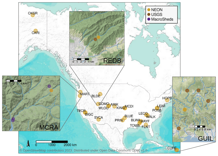
Figure 1 Map of target sites (NEON) and donor gauge candidates for three target sites: MCRA (McRae Creek, state of Oregon), REDB (Red Butte Creek, state of Utah), and GUIL (Rio Guilarte, Puerto Rico). © OpenStreetMap contributors 2023. Distributed under the Open Data Commons Open Database License (ODbL) v1.0.

2.3 Target sites

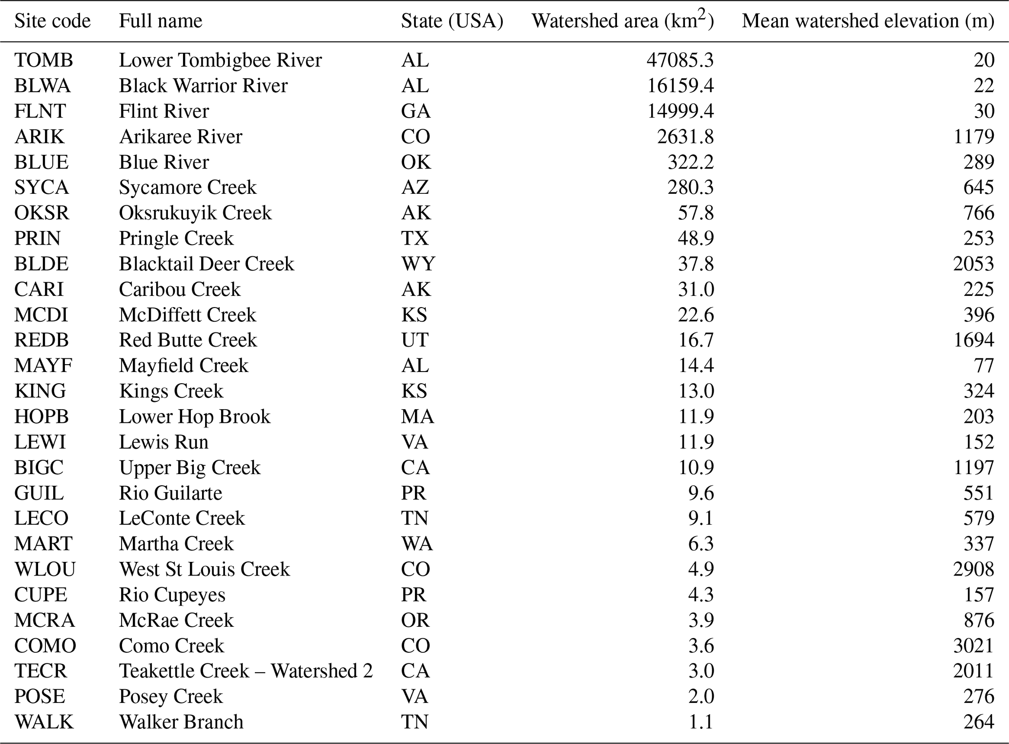
All 27 lotic (flowing) aquatic sites associated with NEON were included as target sites for discharge prediction in this study (Fig. 1). The sites TOMB, BLWA, and FLNT are installed on major rivers, downstream of hydropower dams. All other sites have been free of any dam influence since 2012 at the latest, and are designated “wadeable streams” by NEON. In addition to the three sites above, hydrology at BLUE, GUIL, KING, MCDI, and ARIK may be influenced by agricultural activity, especially in the relatively arid Midwest (i.e., the states KS, CO, and OK). Continuous discharge data for TOMB are provided by a nearby gauge of the US Geological Survey's National Water Information System, and are given at hourly intervals, rather than at NEON's customary 1 min intervals.

Table 1 Target sites for discharge prediction. See https://www.neonscience.org/field-sites (last access: 15 Julu 2023) for more information.

2.4 Linear regression and model selection

All donor and response discharge time series were neglog transformed (Eq. 1; Whittaker et al., 2005) before fitting linear regression models.

$$\begin{array}{}\text{(1)}& x_{\mathrm{neglog}}=\mathrm{sign}\left(x\right)\log (\left|x\right|+\mathrm{1})\end{array}$$

Series were scaled by 1000 before transformation, in order to reduce the disproportionate impact of adding one to every value. Response observations were synchronized to the interval of the predictor series by approximate datetime join, allowing forward or backward timeshifts of up to 12 h if necessary.

One of three forms of linear regression was employed at each site, depending on the number and location of donor gauges and the donor–target gauge relationships. For sites with a single donor gauge (REDB, HOPB, BLUE, SYCA, LECO), the considered predictors were discharge from the donor gauge, a four-season categorical variable, and their interaction. Additionally, an intercept parameter could be estimated, or not, for each specification. Thus, up to six models were fitted using OLS regression (Galton, 1886), ensuring at least 15 observations per model parameter. At LECO, an additional dummy variable was included to address an intercept change due to a wildfire in November 2016. The best model was selected via 10-fold cross-validation, minimizing the mean squared error (MSE). MSE, being a squared-error term, disproportionately penalizes the inaccurate prediction of high discharge values and helps to balance against the relative rarity of high discharge measurements in the field data. At site SYCA, the log-log relationship between discharge at the target gauge and a single donor gauge exhibited a distinct breakpoint, and segmented least-squares regression was used (R package “segmented”; Muggeo, 2008). At all other sites (19 in total), predictors included discharge series from 2–4 donor gauges, season, and all interactions. To control overfitting and shrink covarying coefficients toward zero, we used L2 regularization (ridge regression; Gruber, 2017) via the R package “glmnet” (Friedman et al., 2010). As with the other regression approaches, 10-fold cross-validation and MSE loss were used for model parameter selection – in this case for the value of the penalty hyperparameter λ, which was set to the mean across folds of λ producing the minimum cross-validated error. Unlike OLS and segmented regression, ridge regression uses biased estimators that complicate the calculation of prediction intervals. We generated 95 % prediction intervals for ridge regression discharge estimates using the 95th percentiles of 1000 bootstrap predictions at each prediction point, which were generated from 1000 resamples of the fitting data stratified by season. We emphasize that these prediction intervals should be conservative estimates of the true uncertainty, as they do not fully account for uncertainty due to bias (Goeman et al., 2012).

For each site, we fitted two sets of models as described above, one with discharge scaled by watershed area (i.e., “specific discharge” in the surface water hydrology sense) prior to transformation and one without areal scaling. Only one model from each set was ultimately selected for each target site; this was done on the basis of the Kling–Gupta efficiency (KGE; Gupta et al., 2009), a composite model efficiency metric that incorporates measures of correlation, variance, and bias. We also report the percent bias and Nash–Sutcliffe efficiency (NSE; Nash and Sutcliffe, 1970), a measure of predictive accuracy that implicitly compares predictions to a mean-only reference model.

Predictions were generated for all time points during which data were available at the selected donor gauges. At target site COMO, a secondary model omitting one donor gauge was able to produce 36 % more predictions than the selected model, so our predicted discharge at COMO is a composite of both models, with the better model's predictions preferred where available. We were unable to locate sub-daily donor gauge data near COMO, so regression predictions for this site were generated at daily intervals. Regression predictions for all other sites were generated at sub-daily intervals matching the coarsest interval across predictor gauges – generally 15 min, though it should be noted that in most cases these predictions were interpolated to 5 min for our composite discharge product.

2.5 Neural network setup and operation

Supplementing the linear regression methods described above, we simulated discharge data at all 27 target sites using long short-term memory recurrent neural networks (LSTM-RNNs; hereafter “LSTMs”; Hochreiter and Schmidhuber, 1997). Four LSTM strategies were employed, all of which involved training on a large and diverse corpus of stream discharge data (Table 3). Two of these strategies included further finetuning to the time-series dynamics of each target site in turn. Due to the relative scarcity of field-measured discharge observations (between 39 and 213 per site; mean 122), none were used in LSTM training. Instead, these measurements were used only to evaluate predictions. LSTMs trained in this study are intended only for discharge prediction within the temporal and spatial bounds of NEON's early operational phase, not for forecasting or application to other sites. Therefore, all available daily training data were used as such; no validation set was kept for hyperparameter tuning, and no holdout set of daily estimates was kept for evaluation (note that split-sample designs may be undesirable more generally: Arsenault et al., 2018; Guo et al., 2018; Shen et al., 2022). See Kratzert et al. (2019b) and Read et al. (2019) for split-sample considerations in the context of a generalist and process-guided generalist LSTM, respectively.

After a hyperparameter search routine, described below, potentially skilled models were identified as those achieving at least 0.5 KGE and 0.4 NSE. The best-performing potentially skilled LSTM for each site (if applicable) was then re-trained 30 times, forming an ensemble. Ensembles were trained for 18 of 27 sites. LSTM predictions included in our composite discharge product are means taken across the distributions of ensemble point predictions. Uncertainty bounds were computed as the 2.5 % and 97.5 % quantiles of these distributions. LSTM skill was evaluated on the basis of mean ensemble efficiency (KGE) with respect to field-measured discharge (Table A1).

Daily discharge time series (training data) and field-measured discharge were scaled by watershed area. For each predicted day, LSTMs received five dynamic Daymet meteorological forcing variables and 11 static watershed attribute summary statistics (Table 2). Multitask learning (Caruana, 1998; Sadler et al., 2022) was found to improve discharge prediction broadly in a preliminary analysis, so Daymet minimum air temperature was used as a secondary target variable. Kratzert et al. (2019a) found that a maximum of about 150 preceding days were able to influence the LSTM output in a similar prediction problem, so we set the input sequence length to 200 d to ensure full utilization of available information. In other words, for each day of prediction, the model was able to leverage information from the preceding 200 d.

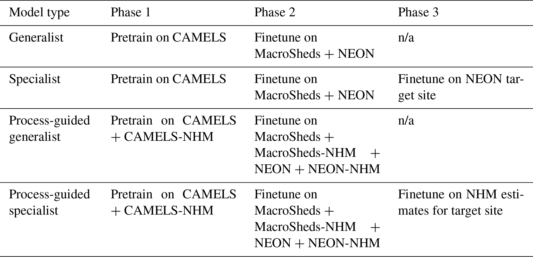
We employed the four different training pipelines described in Table 3. Of the 671 CAMELS watersheds (i.e., basins), we used a subset of 531 with undisputed areas of less than 2000 km² (Newman et al., 2017). For finetuning data, we used version 1 of the MacroSheds dataset (Vlah et al., 2023a). We excluded MacroSheds sites outside North America and those with a coastal or urban hydrological influence, for a total of 133 sites out of the 169 that are currently available. We chose MacroSheds sites for finetuning because the MacroSheds and NEON datasets focus primarily on small watersheds, often smaller than 10 km² in area, while only eight CAMELS watersheds are smaller than 10 km² and most are larger than 100 km² (Vlah et al., 2023a). The daily mean discharge computed from NEON's continuous discharge product was used, but only for those site-months deemed Tier 1 or Tier 2 by Rhea et al. (2023a), alongside MacroSheds data for finetuning.

For the process-guided strategies, we used NHM estimates for all reaches coinciding with a CAMELS or MacroSheds gauge, for a total of 551 reaches. Only nine target sites on relatively high-order streams were amenable to the process-guided specialist approach, as these sites are on reaches large enough to be modeled by the NHM. The most recent version of the NHM at the time of this writing provides discharge estimates beginning in 1980 and ending in 2016, just before the installation of most NEON target sites.

Table 2 LSTM input data. ^*Attribute tested as an afterthought but not included in this study due to a negligible improvement in the trial parameter search.

Table 3 LSTM model training pipelines used in the simulation of discharge at target sites. Here, “NEON” refers to NEON's continuous discharge product, RELEASE-2023, with quality-flagged estimates and < Tier-2 site-months (according to Rhea et al., 2023a) removed. n/a – not applicable.

LSTMs were configured in R and trained using v1.3.0 of the NeuralHydrology library in Python (Kratzert et al., 2022; Van Rossum and Drake, 2009) on the Duke Compute Cluster at Duke University, Durham, NC, USA. All trained models used the Adam optimizer (Kingma and Ba, 2014) and NeuralHydrology's “NSE loss” function after an initial evaluation in which we compared it to the MSE and root mean squared error (Table 4). Learning was annealed using a series of three fixed rates for pretraining and for round one of finetuning according to Eq. (2):

$$\begin{array}{}\text{(2)}& r=\left\{\begin{array}{ll}a,& e\mathit{ϵ}\mathit{\{}\mathrm{0},\mathrm{\dots },[\frac{E}{\mathrm{3}}\left]\mathit{\right\}}\\ \frac{a}{\mathrm{10}},& e\mathit{ϵ}\mathit{\left\{}\right[\frac{E}{\mathrm{3}}],\mathrm{\dots },[\frac{\mathrm{2}E}{\mathrm{3}}\left]\mathit{\right\}}\\ \frac{a}{\mathrm{100}},& e\mathit{ϵ}\mathit{\left\{}\right[\frac{\mathrm{2}E}{\mathrm{3}}],\mathrm{\dots },E\mathit{\}},\end{array}\right.\end{array}$$

where r is the learning rate, a is any power of 10 between 0.1 and 10⁻⁷, and E is the number of training epochs. Learning rate was annealed using a series of two fixed rates for round two of finetuning according to Eq. (3):

$$\begin{array}{}\text{(3)}& r=\left\{\begin{array}{ll}\frac{a}{\mathrm{10}},& e\mathit{ϵ}\mathit{\{}\mathrm{0},\mathrm{\dots },[\frac{E}{\mathrm{2}}\left]\mathit{\right\}}\\ \frac{a}{\mathrm{100}},& e\mathit{ϵ}\mathit{\left\{}\right[\frac{E}{\mathrm{2}}],\mathrm{\dots },E\mathit{\}}.\end{array}\right.\end{array}$$

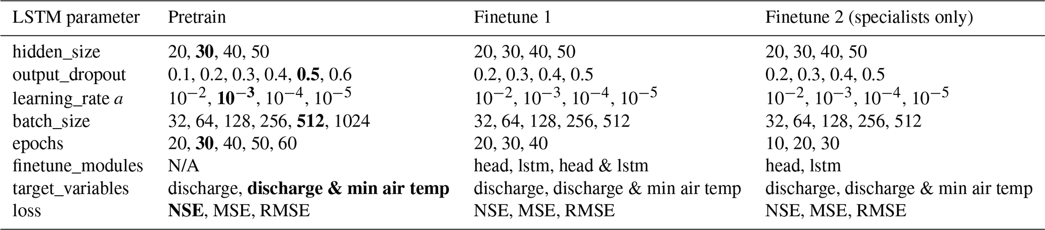
Learning rate and other hyperparameters were selected via an inexhaustive (pseudo) grid search (Table 4), i.e., we specified a sequence of possible values for each hyperparameter and randomly selected from them to specify 30 models for each generalist. For each site, one specialist model was then configured to further finetune each of the 30 generalists, again using a partial grid search to define any mutable hyperparameters. Otherwise, hyperparameters were inherited from the previous training period (Table 4). Due to our incomplete hyperparameter search procedure, better combinations probably exist. We elected not to exhaustively pursue optimal hyperparameter combinations due to the computational demand of a full grid search and a lack of access via NeuralHydrology to callback methods necessary for implementation of a true random search (Bergstra and Bengio, 2012).

Table 4 LSTM hyperparameter search space for all model types, and the selected values (bold) used for pretraining. These were observed to allow for both malleability and high performance of subsequent finetuning iterations over nearly 2000 exploratory LSTM trials. The relationship of a to learning_rate is defined in Eqs. (2) and (3). See the NeuralHydrology documentation for parameter definitions: https://neuralhydrology.readthedocs.io/en/latest/usage/config.html (last access: 25 May 2023).

All LSTM models were outfitted with fully connected, single-layer embedding networks to efficiently encode inputs as fixed-length numerical vectors (Arsov and Mirceva, 2019). Separate embedding networks were used for static and dynamic inputs, with 20 neurons for static inputs and 200 neurons for dynamic inputs. All embedding neurons used the hyperbolic tangent activation function. Another advantage of embedding networks in the context of the NeuralHydrology library is that they provide one of few opportunities to introduce dropout, which can improve training efficiency and reduce overfitting (Srivastava et al., 2014).

2.6 Composite discharge data product

This study generated time-series predictions of discharge for each lotic NEON site using up to three distinct processes: linear regression on absolute discharge, linear regression on specific discharge, and one of four LSTM strategies. We provide regression predictions wherever applicable (24 of 27 sites). LSTM predictions are provided only for sites that had promising model performance after a hyperparameter search and for which ensemble models were therefore trained (18 of 27). All model outputs and results from this study are archived at https://doi.org/10.6084/m9.figshare.c.6488065 (Vlah et al., 2023c).

In addition to predictions from individual modeling strategies, we provide an analysis-ready discharge dataset for all 27 sites that splices the best available predictions across methods – including published NEON estimates (NEON, 2023a) – into composite series (https://doi.org/10.6084/m9.figshare.c.6488065, Vlah et al., 2023c), which can be visualized interactively at https://macrosheds.org/data/vlah_etal_2023_composites/ (last access: 3 February 2024). Composite series for each NEON site begin at the start of site operation and extend to at most 30 September 2021, the last date included in the 2023 release of NEON's continuous discharge product. We also provide individual model predictions extending through 2022. A complete list of products from this study, and their links, can be found in Table A3.

To construct composite series, we first distinguished “good” site-months of NEON discharge estimates as those categorized as Tier 1 or Tier 2 by Rhea et al. (2023a). For a NEON site-month to meet the requirements for at least Tier 2, four requirements must be met. The linear relationship between stage, determined from pressure transducer readings, and field-measured gauge height must score at least 0.9 NSE. The transducer-derived stage series must also pass a drift test relative to gauge height, but only if sufficient data exist to perform such a test. The rating curve used to relate stage to discharge must score at least 0.75 NSE, and fewer than 30 % of predicted discharge values may exceed the range of measured discharge used to build the curve. See Rhea et al. (2023a) for further details.

Although only 50 % of NEON's RELEASE-2023 estimates are classified as Tier 1 or Tier 2, the remainder may still be of high analytical value if NEON's quality control indicators and uncertainty bounds are observed. We also stress that NEON rating curves and protocols improved over the course of its early operational phase and continue to do so.

We then ranked the available predictions for each site, assigning a rank of 1 either to predictions from linear regression or to NEON's continuous data product, depending on the overall KGE and NSE against the field-measured discharge. KGE was considered first and used to determine preference, except in cases where the difference between NSE scores was greater than that between KGE scores and opposite in sign. Rank 2 predictions were then used to fill gaps of 12 or more hours in the rank 1 series, but only “good” NEON site-months were included. Only after this first round of gap-filling were the remaining NEON data incorporated, with site-years achieving at least 0.5 KGE and 0.5 NSE against the field-measured discharge being used to fill still-remaining gaps. Finally, daily LSTM predictions (placed at 12:00:00 UTC on the day of prediction) were used to fill any recalcitrant gaps, but only if produced by an ensemble model achieving at least 0.5 KGE and 0.5 NSE across all field discharge observations. Note that while such benchmarks are in common use (Moriasi et al., 2015), the efficiency that any model can or should achieve varies substantially with the hydroclimate and watershed characteristics of a given site (Seibert et al., 2018). We provide all data and code for modifying the composite discharge product in accordance with alternative benchmarks as users see fit. After visual examination of composite series plots, we chose to prefer NEON predictions to linear regression predictions at site ARIK, “good” or not, due to frequent sharp discontinuities between the two predicted series. See Table A1 for an account of the linear regression and LSTM methods used in the construction of ensemble series.

The prevailing interval varies across data sources used to assemble our composite discharge product from 1 min (NEON) to 1 d (LSTM predictions; regression predictions at site COMO). Regression predictions were primarily generated at 15 min intervals, and their timestamps are always divisible by 15 min. Around the prevailing NEON interval there is considerable variation due to data gaps and sensor reconfigurations, both across sites and across the temporal ranges of each site's record. To reduce the complexity associated with irregular time-series analysis, we synchronized the interval across data sources to 5 min. Regression estimates were linearly interpolated to 5 min, though gaps larger than 15 min were not interpolated. NEON estimates were first smoothed with a triangular moving average window of 15 min to remove unrealistic minute-to-minute noise associated with Bayesian error propagation. They were then interpolated the same way as the regression estimates and finally downsampled to 5 min, with some timestamps being shifted by up to 2 min. For example, for a sampling duration of 30 min, a sample taken at 00:03:00 would be shifted by 2 min by rounding each timestamp up to the nearest minute divisible by 5.

3 Results

A performance comparison of linear regression on discharge from donor gauges and four LSTM strategies is shown in Figs. 2 and A1 and detailed in Table A1. Via linear regression, we were able to produce 15 min discharge estimates at 11 sites with overall KGE scores higher than those of published series (Fig. 2). At four of the same sites, we achieved a higher KGE via LSTM methods, which generated daily discharge series. Of the 10 sites at which the published discharge KGE was less than 0.8, we improved five sites to above that mark (mean 0.932, n=5).

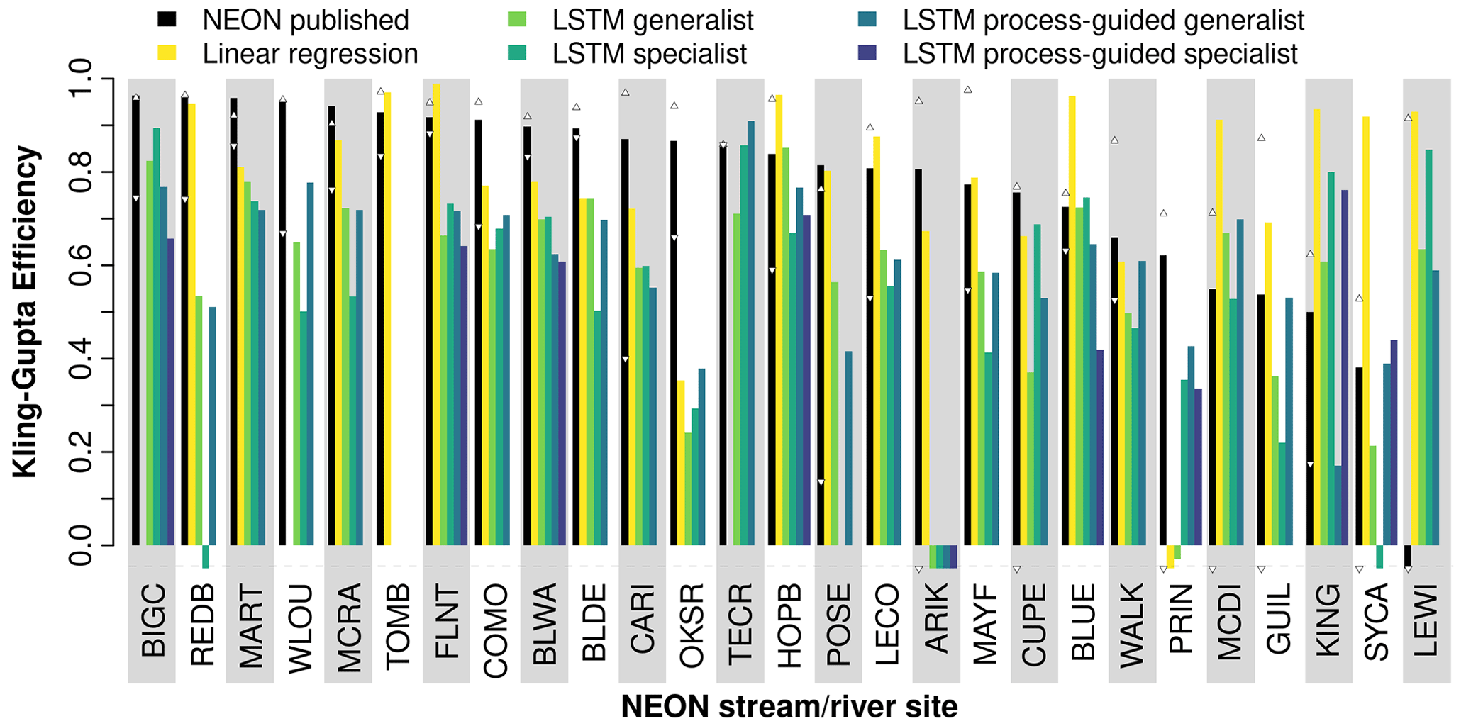
Figure 2 Efficiency of five stream discharge prediction methods and NEON's published continuous discharge product at 27 NEON gauge locations versus field-measured discharge. Small, white triangles represent the max/min KGE of the published discharge by water year (1 October through 30 September) with at least five field measurements (or two for site OKSR). KGE was computed on all available observation–estimate pairs except those with quality flags (dischargeFinalQF or dischargeFinalQFSciRvw of 1). For the best-performing LSTM method at all sites except TECR, FLNT, REDB, WALK, POSE, and KING, the displayed KGE is averaged over 30 ensemble runs with identical hyperparameters. For the sites just named, the performance of a chosen method after ensembling dropped below that of at least one other method's optimal KGE from the parameter search. For all other LSTM site–method pairs, which were not ensembled, the displayed performance is that of the best model trained during the parameter search phase. Sites are ordered by the KGE of the NEON continuous discharge. See Table 3 for LSTM model definitions. A KGE of 1 is a perfect prediction, while a KGE of −0.41 is similar in skill to prediction from the mean. Negative values are truncated at −0.05 in this plot to improve visualization.

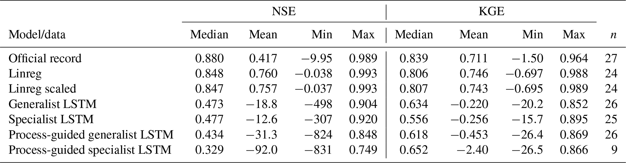
For 12 of 27 sites, linear regression on specific discharge (i.e., scaled by watershed area) provided the most accurate discharge predictions, while linear regression on absolute discharge performed better at the other 12 sites with donor gauges. LSTM models (as proper ensembles) outperformed linear regression at only two sites. In general, linear regression provided more accurate predictions than all LSTM methods. Linear regression on absolute discharge produced estimates with a median NSE of 0.848 and a median KGE of 0.806 across sites (n=24; Table 5). Linear regression on specific discharge produced similar median scores (Table 5), but with deviations of up to 0.05 NSE and 0.08 KGE at individual sites.

Table 5 Performance of five stream discharge prediction methods, and the official continuous discharge time-series data, across n of 27 NEON gauge locations (final column). For both the Nash–Sutcliffe and Kling–Gupta efficiency coefficients, a value of 1 indicates perfect prediction. A value of 0 NSE indicates that the predictive skill is equivalent to prediction from the mean, while a negative NSE is worse than mean prediction. This threshold lies at approximately −0.41 for KGE (Knoben et al., 2019). “Linreg” is linear regression on the donor gauge discharge series, and “scaled” means that the predictor and response discharge were scaled by their respective watershed areas.

Linear regression was not applicable at sites TECR, BIGC, or WLOU due to the lack of donor gauges contemporary with target gauge data. Donor gauges associated with Kings River Experimental Watersheds exist within close proximity to TECR and BIGC, but we were unable to access up-to-date discharge records for these gauges.

The process-guided specialist LSTM yielded predictions on par with those of the other LSTM strategies in terms of KGE (median 0.652; n=9), but performed worst of the four in terms of NSE (median 0.329; n=9). Conversely, the specialist performed better than the generalist in terms of NSE but not KGE. The process-guided specialist LSTM strategy was viable at nine sites for which discharge estimates were available from the National Hydrologic Model.

In addition to improvements in accuracy, estimates from this study inform ∼5981 site-days (75 %) of missing data in the official discharge record (Fig. 3), though it should be noted that they also omit ∼4486 site-days otherwise present in NEON's official record. Omissions occur wherever observations are missing from the records of one or more donor gauges, and LSTM methods did not achieve the desired efficiencies. Approximately 1221 site-days are missing from the official record and from our reconstructions.

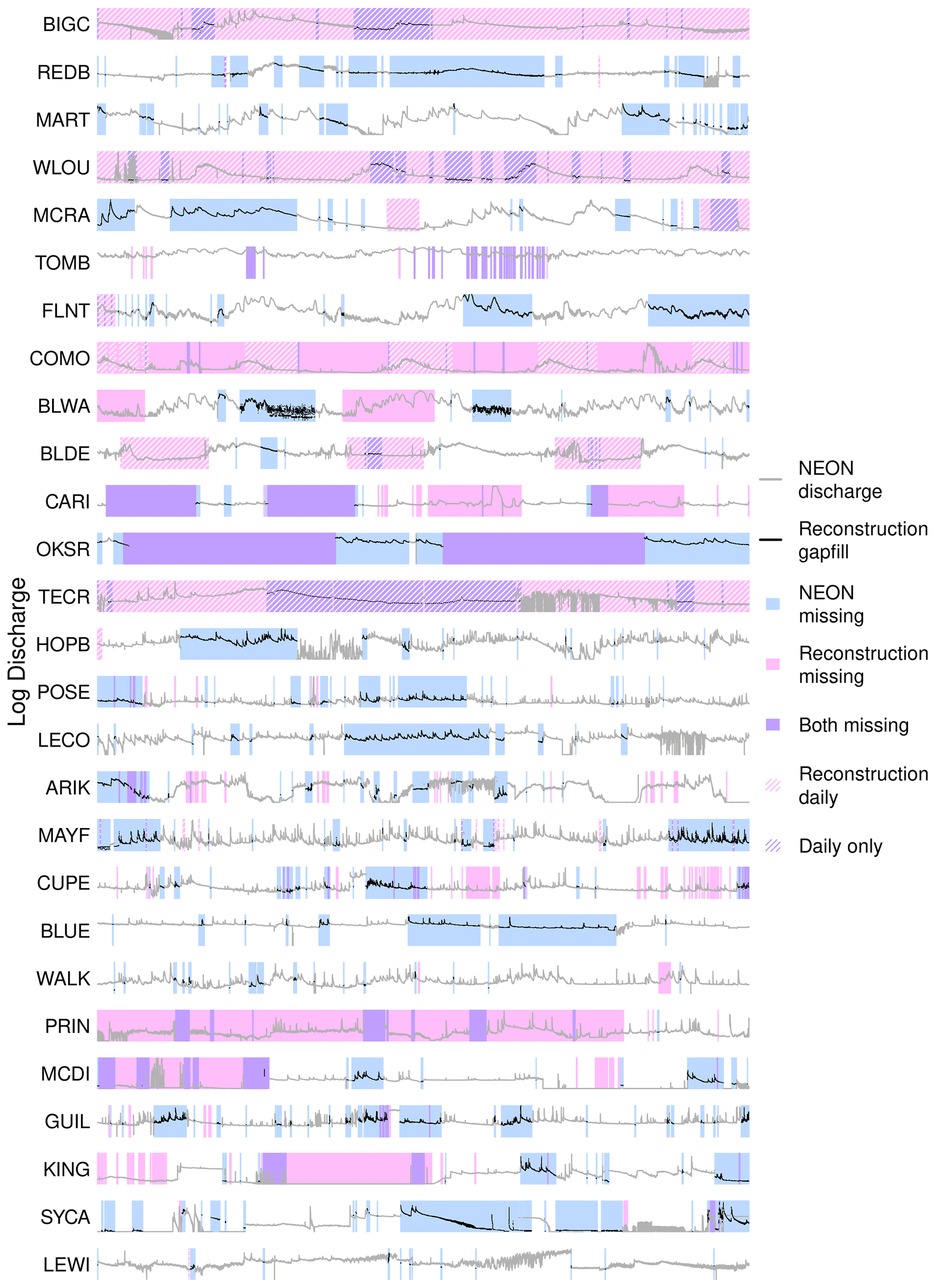
Figure 3 Durations of missing values (gaps) in NEON's 2023 release of continuous discharge time series, illustrating gaps filled or informed by estimates from this analysis. All officially published values are shown, including those with quality control flags. Sites are ordered as in Fig. 2. Gaps smaller than 6 h are not indicated. Figure A10 is the same, but with a fixed and labeled x axis.

Estimated discharge time series from this study are of practical value for any researcher using NEON continuous discharge data, especially for those sites and site-months at which published data from NEON's early operational phase may be unreliable (Rhea et al., 2023a). Figure 4 shows that official records at sites REDB and LEWI are compromised by disagreements (erratic sections of gray lines) between pressure transducer stage readings and manual gauge height recordings, as discussed in Rhea et al. (2023a). Red lines show improved estimates via linear regression on discharge from donor gauges. Sites FLNT and WALK show generally close agreement between NEON discharge and our regression estimates, but the uncertainty associated with high discharge values should be noted.

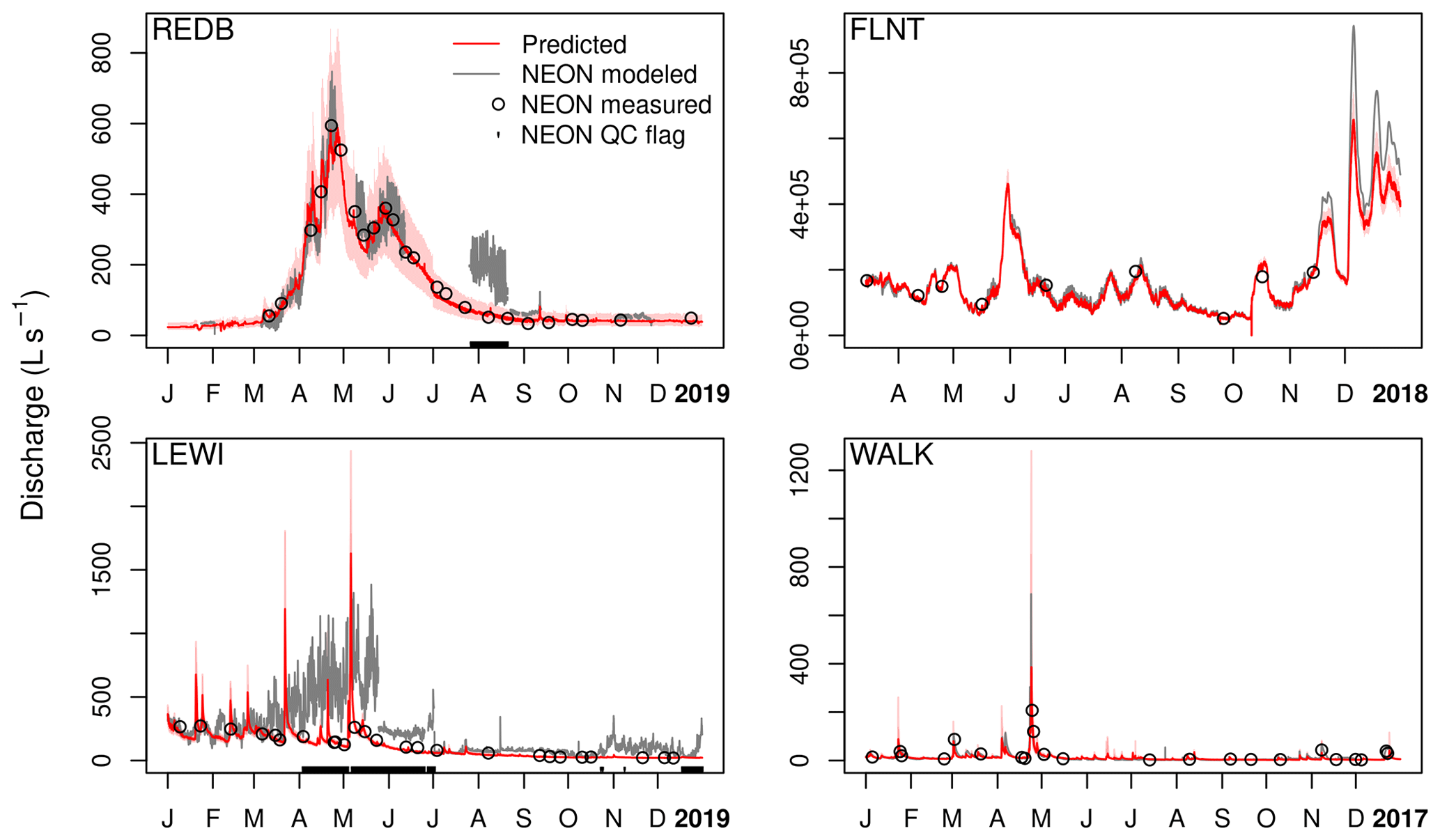
Figure 4 Best linear regression predictions of continuous discharge for four NEON gauge-years compared with official NEON discharge data. All officially published values are shown, including those with quality control flags, indicated by black marks on the lower border. Light red bands represent 95 % prediction intervals. NEON uncertainty is not shown.

4 Discussion

This study was designed to produce high-quality estimates of continuous discharge for NEON stream gauges, especially at 10 gauges for which the KGE of published continuous discharge was lower than 0.8, over the full record, when compared to field-measured discharge. A secondary goal was to improve temporal coverage of the official discharge record where possible.

We treat NEON field-measured discharge as truth, which means there are 39–213 observations for each target site. Although these numbers represent a tremendous investment of time and technical effort, they do not meet the high data volume requirements for most machine learning approaches, so we used field discharge only to evaluate, rather than train, LSTM models. By contrast, in linear regression, regardless of the details of any particular method, we ultimately fit a line to the relationship between donor gauge data and field measurements at each target site. Because the linear regression models are allowed to “see” all of the target site data (after a model is selected via cross-validation), they have a powerful advantage over the LSTM approaches, which in this context must essentially treat target watersheds as if they are ungauged. Furthermore, whereas the LSTM models must parameterize each day of prediction individually, the regression models need only parameterize relationships between flow regimes. Still, if given enough training data, including examples of watersheds and streams similar to each of those modeled in this study, the LSTM approaches would eventually close the performance gap. See Figs. A2, A3, A4, A5, A7, and A8 for linear regression diagnostics.

In this study, discharge estimates produced by linear regression were more accurate than those generated by LSTM models in 21 of 23 comparisons (Fig. 2). This demonstrates the value of existing gauge networks in advancing discharge estimation at newly or partially gauged locations; however, there is a limit to the predictive potential of linear regression methods, as they depend on a strong correlation between streamflow at target and donor gauges. In principle, there is no such limit for machine learning approaches, which are instead limited by the quality and quantity of training data.

The process-guided specialist LSTM yielded predictions on par with those of the other LSTM strategies in terms of KGE, but performed worst of the four in terms of NSE, possibly indicating that information gleaned from NHM estimates helped this strategy to accurately capture discharge variance and reduce prediction bias without ultimately improving the correlation between predictions and observations. Unlike KGE, NSE only explicitly captures this latter metric (Nash and Sutcliffe, 1970; Gupta et al., 2009). Conversely, the specialist performed better than the generalist in terms of NSE but not KGE, suggesting that information contained in NEON's continuous discharge product was of disproportionate predictive value relative to each of correlation, variance, and bias, favoring correlation.

The specialist may have been affected by data filtering choices. After filtering NEON continuous discharge for rating curve issues, drift, and quality flags, relatively few daily estimates were available for some sites (47–1642). Annual and seasonal variation in meteorological forcings and discharge in NEON sites' generally small, often mountainous watersheds may be large enough that finetuning a pretrained LSTM on a few hundred days of site-specific data reduces its ability to generalize at that site. Our specialist LSTM strategy in particular might be improved with a broader hyperparameter search, especially one that explores smaller learning rates. Ideally, site-specific finetuning should enable better prediction by allowing the network to assimilate information unique to the target site without corrupting previously learned generalities. For validation plots of all ensembled LSTMs, see Fig. A6.

The process-guided specialist LSTM strategy was viable at nine sites for which discharge estimates were available from the National Hydrologic Model. By using a mechanistic (i.e., process-based) model with higher spatial resolution than the NHM, it should be possible to apply this process-guided approach at more of the NEON sites. A potentially stronger process-guided approach would use mechanistic model predictions as features (predictors), rather than training targets, but that would require mechanistic model predictions concurrent with discharge series at target sites, whereas NHM predictions at the time of this writing are available only through the year 2016. For a summary of process-guided deep learning strategies, see the “Integrating Design” subsection of Appling et al. (2022).

We caution that evaluation scores for both NEON's published estimates and ours are computed on a small fraction of each series for which both an estimate and a direct field measurement are available (39–213 per site), and that measurements tend to be collected disproportionately at low flow. This often occurs for practical reasons such as site access and technician safety, but may also reflect a need to characterize the low-flow variability of the stage–discharge relationship in streams with unstable low-flow hydrologic controls, such as unconsolidated bed material.

Whatever the reason for less sampling at high flow, any model attempting to use field measurements to reconstruct continuous discharge will estimate with greater uncertainty at high flow than at low, and users of our composite discharge product should observe uncertainties associated with estimates from all methods. Mechanistic models that proceed from physical principles, or data-driven approaches that can generalize from prior observations, do not in principle suffer this disadvantage, as they do not depend on observations from a target site. However, these approaches may not reliably generate strong predictions at all sites or under all conditions (Razavi and Coulibaly, 2013; Kratzert et al., 2019b), and may produce erratic point estimates where conditions diverge from past observations. Hybrid approaches that successfully leverage field measurements, as well as physical principles or learned relationships, are likely to yield well-constrained predictions where our efforts did not.

This study demonstrates that, in proximity to established streamflow gauges, even simple statistical methods can be used to generate accurate, continuous discharge at “virtual gauges” where discrete discharge has been measured. The number of field measurements across sites in this study varies from 39 to 213, but the number required for virtual gauging may be substantially smaller than even the minimum of this range. If the discharge relationships between a target site and all donor gauges were perfectly linear or log-linear, they could in principle be established with only two precise measurements at the target site. More important than the quantity is the distribution of measurements across flow conditions, which should be sufficient to fully characterize all modeled discharge relationships and their linearity or lack thereof (Sauer, 2002; Zakwan et al., 2017). Concretely, we advocate for “storm chasing”, or disproportionately seeking to sample discharge under high-flow conditions and during both rising and falling limbs of storm events, rather than routine sampling. Observed NEON flow conditions relative to predicted discharge can be seen in Fig. A9. See Philip and McLaughlin (2018) for further commentary on establishing a virtual gauge network, and see Seibert and Beven (2009) and Pool and Seibert (2021) for information on the number and statistical properties of discharge samples required to establish strong stage–discharge or discharge–discharge relationships.

5 Conclusions

Using linear regression on donor gauge data and LSTM-RNNs, we reconstructed continuous discharge at 5 min and/or daily frequency for the 27 stream and river monitoring locations of the National Ecological Observatory Network (NEON) over the water years 2015–2022. Relative to field-measured discharge used as ground truth, our estimates achieve higher Kling–Gupta efficiency than NEON's official continuous discharge at 11 sites. We also provide continuous discharge estimates for ∼199 site-months for which no official values have been published. Estimates from this study can be used in conjunction with officially released NEON continuous discharge data to enhance the analytical potential of NEON's river and stream data products during its early operational phase. Toward that end, we provide composite discharge series for each site, incorporating the best available estimates across all methods used in this study and NEON's published estimates. Considering the lag of up to 2.5 years before provisional discharge data become fully quality controlled and officially released by NEON, our methods may also be used to increase the rate at which discharge-associated stream chemistry, dissolved gas, and water quality products become fully usable by the community. All data and results from this study can be downloaded from the Figshare collection at https://doi.org/10.6084/m9.figshare.c.6488065. Composite series can be visualized interactively at https://macrosheds.org/data/vlah_etal_2023_composites/ (last access: 3 February 2024). All code necessary to reproduce this analysis is archived at https://doi.org/10.5281/zenodo.10067683 (Vlah, 2023b). A complete list of products and URLs can be found in Table A3.

In general, linear regression methods produced more accurate discharge estimates (median KGE: 0.79; median NSE: 0.81; n=24 sites) than LSTM approaches due to the fact that regression models were able to fully leverage available field measurements as well as highly informative donor gauge data. Nonetheless, LSTM methods achieved a median ensemble KGE of 0.71 and an NSE of 0.56 across 18 sites, making their estimates a valuable supplement. Although LSTM-generated discharge series are of daily frequency, some users will prefer them to higher-resolution regression estimates, as the latter may be subject to error in the event of highly localized precipitation events affecting either donor or target gauges, but not both.

Improvements to our design could be made in several ways. LSTM models could be exposed to additional training data, such as the recently published Caravan compendium of CAMELS offshoots (Kratzert et al., 2023) or future expansions of the MacroSheds dataset (Vlah et al., 2023a). Neural networks trained on sub-daily inputs might be better equipped to exploit atmospheric–hydrological dynamics that respond to both daily and annual cycles. Linear regression methods too might be improved with the use of additional predictors, such as continuous water level or precipitation.

The success of simple statistical methods in generating high-quality continuous discharge time series demonstrates the viability of “virtual gauges”, or locations at which a small number of field discharge measurements in proximity to one or more established gauges provide a basis for continuous discharge estimation in lieu of a gauging station. Virtual gauges have the potential to greatly expand the spatial coverage of continuous discharge data throughout the USA and any richly gauged region of the world.

Appendix A

Table A1 Methods from this study used in the construction of composite discharge series. Composite series also incorporate the NEON continuous discharge product DP4.00130.001 (NEON, 2023a). “linreg” is linear regression, “glmnet” is ridge regression, “lm” is OLS regression, “segmented” is segmented regression, “abs” is absolute discharge, “spec” is specific discharge, and “pgdl” is process-guided deep learning.

Table A2 Model input data used in this study.

Table A3 Products of this study.

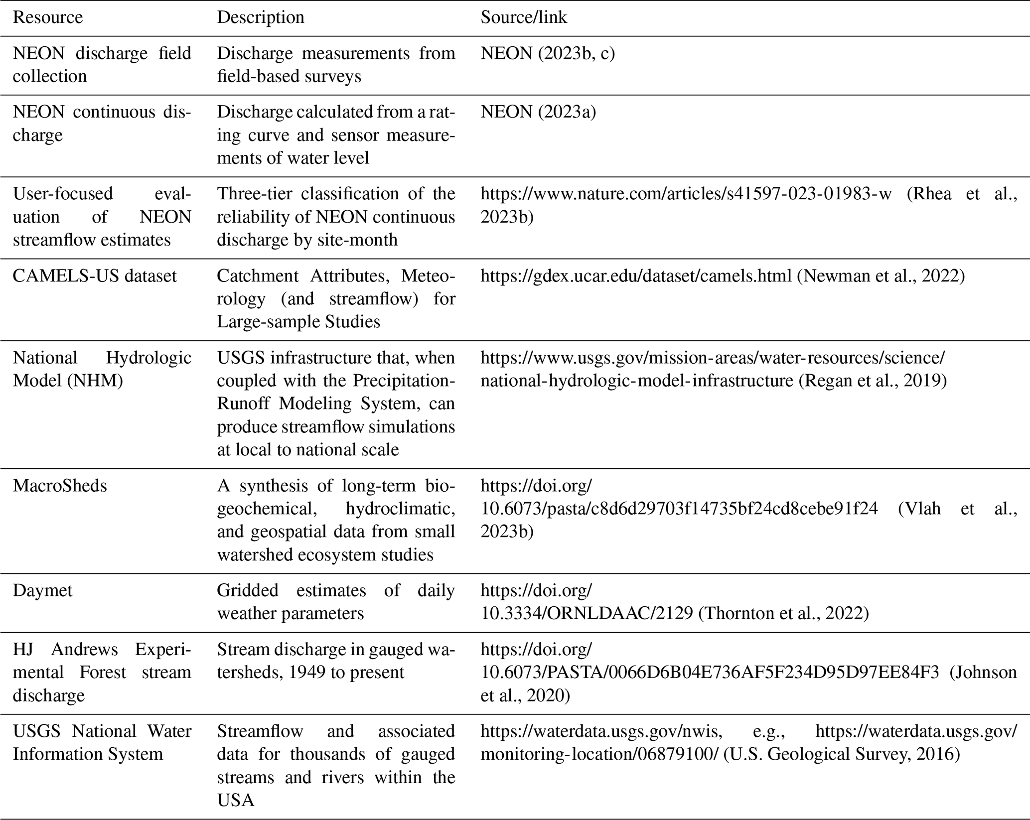
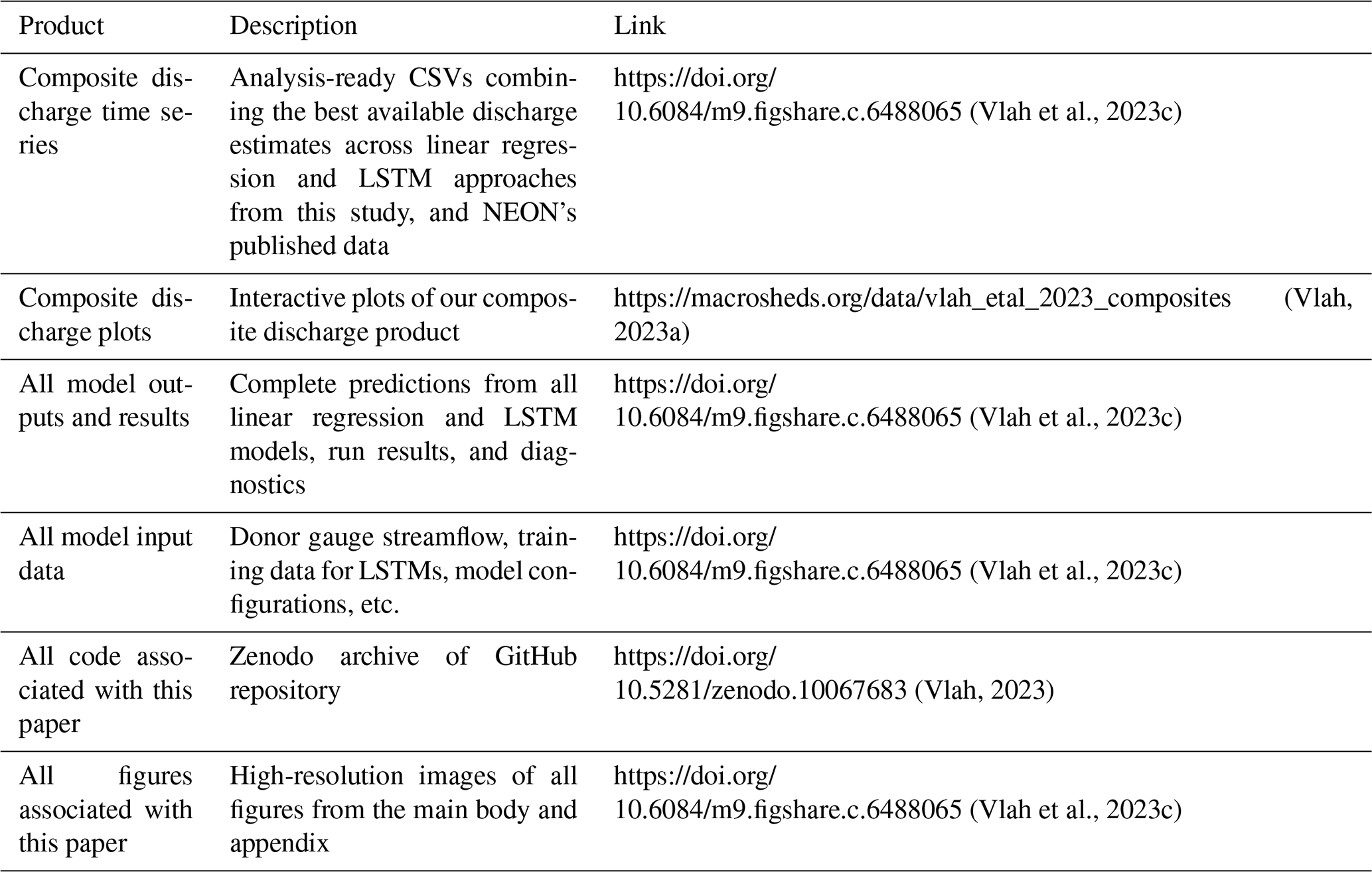
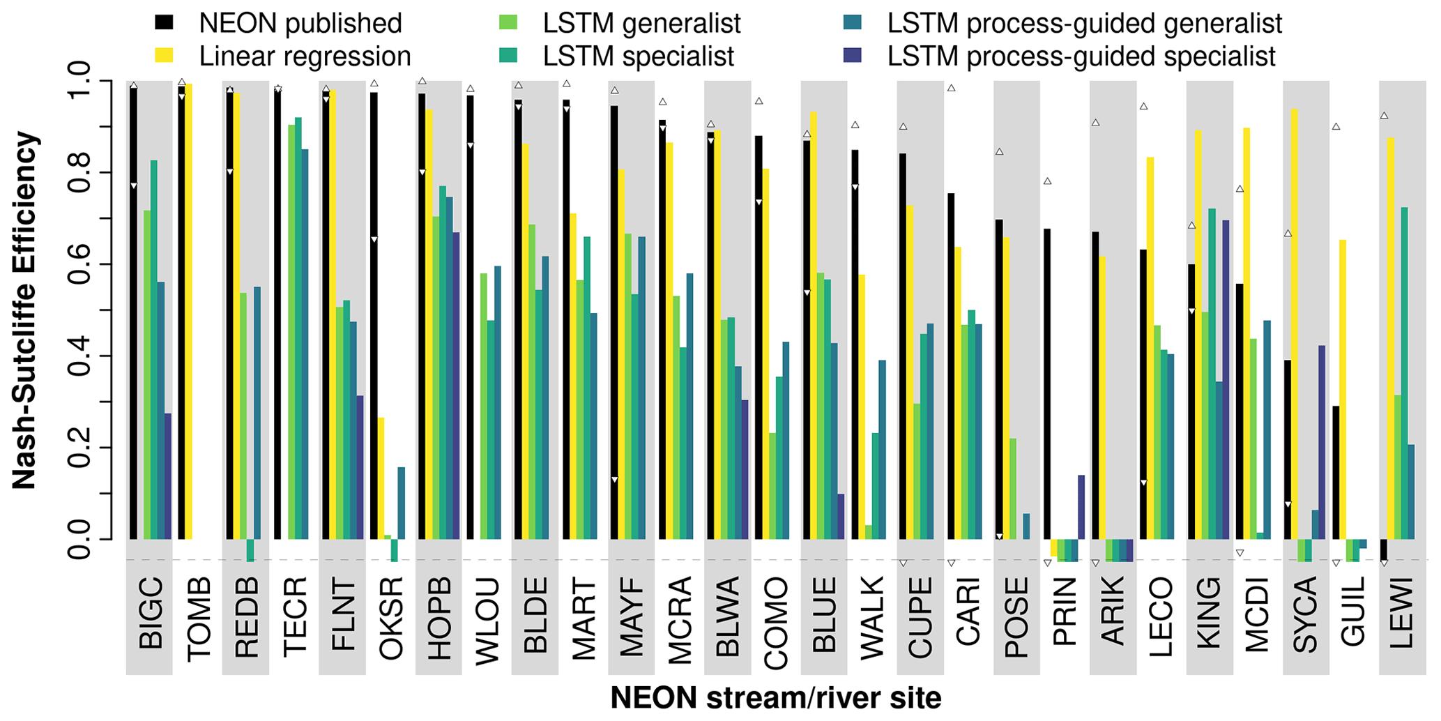
Figure A1 Efficiency of five stream discharge prediction methods and NEON's published continuous discharge product at 27 NEON gauge locations versus field-measured discharge. Small, white triangles represent the max/min NSE of the published discharge by water year (1 October through 30 September) with at least five field measurements (or two for site OKSR). NSE was computed on all available observation–estimate pairs except those with quality flags (dischargeFinalQF or dischargeFinalQFSciRvw of 1). For the best-performing LSTM method, at all sites except TECR, FLNT, REDB, WALK, POSE, and KING, displayed NSE is averaged over 30 ensemble runs with identical hyperparameters. For the sites just named, the performance of a chosen method after ensembling dropped below that of at least one other method's optimal NSE from the parameter search. For all other LSTM site–method pairs, which were not ensembled, the displayed performance is that of the best model trained during the parameter search phase. Sites are ordered by the NSE of NEON continuous discharge. See Table 3 for LSTM model definitions. An NSE of 1 is a perfect prediction, while an NSE of 0 is equivalent in skill to prediction from the mean. Negative values are truncated at −0.05 in this plot to improve visualization.

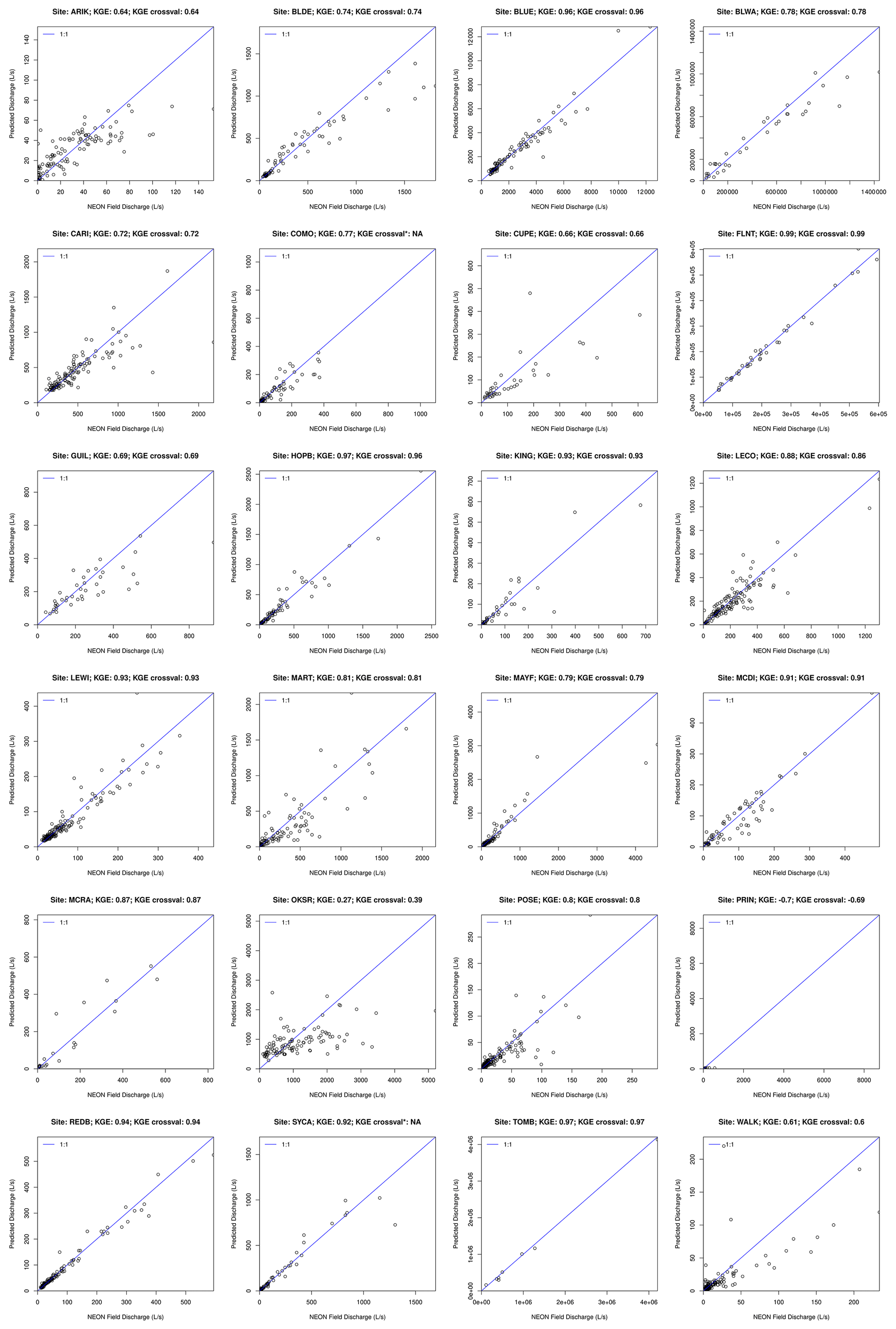
Figure A2 Observed (field) discharge vs. predictions from linear regression on specific discharge (i.e., scaled by watershed area).

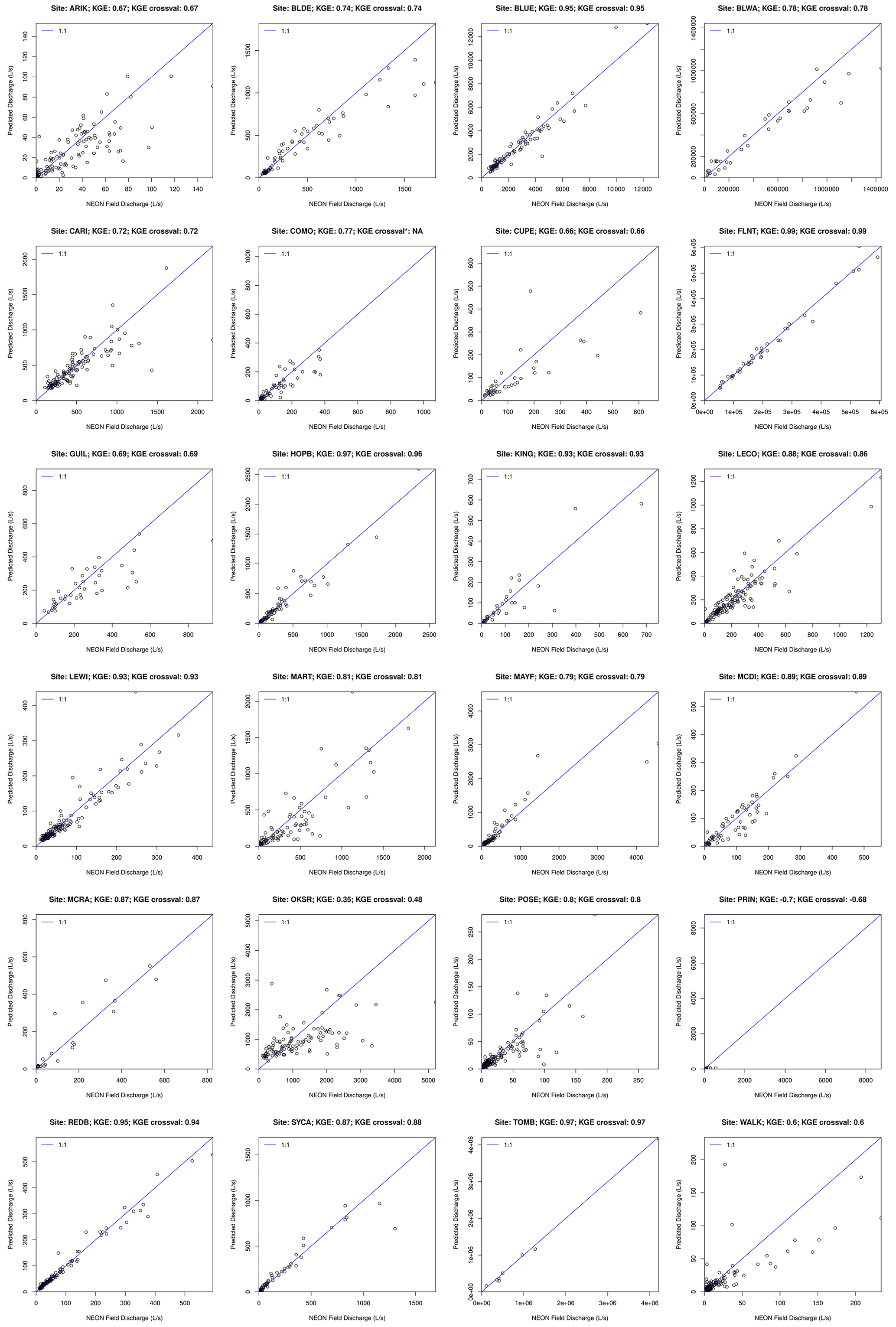
Figure A3 Observed (field) discharge vs. predictions from linear regression on absolute discharge (i.e., not scaled by watershed area).

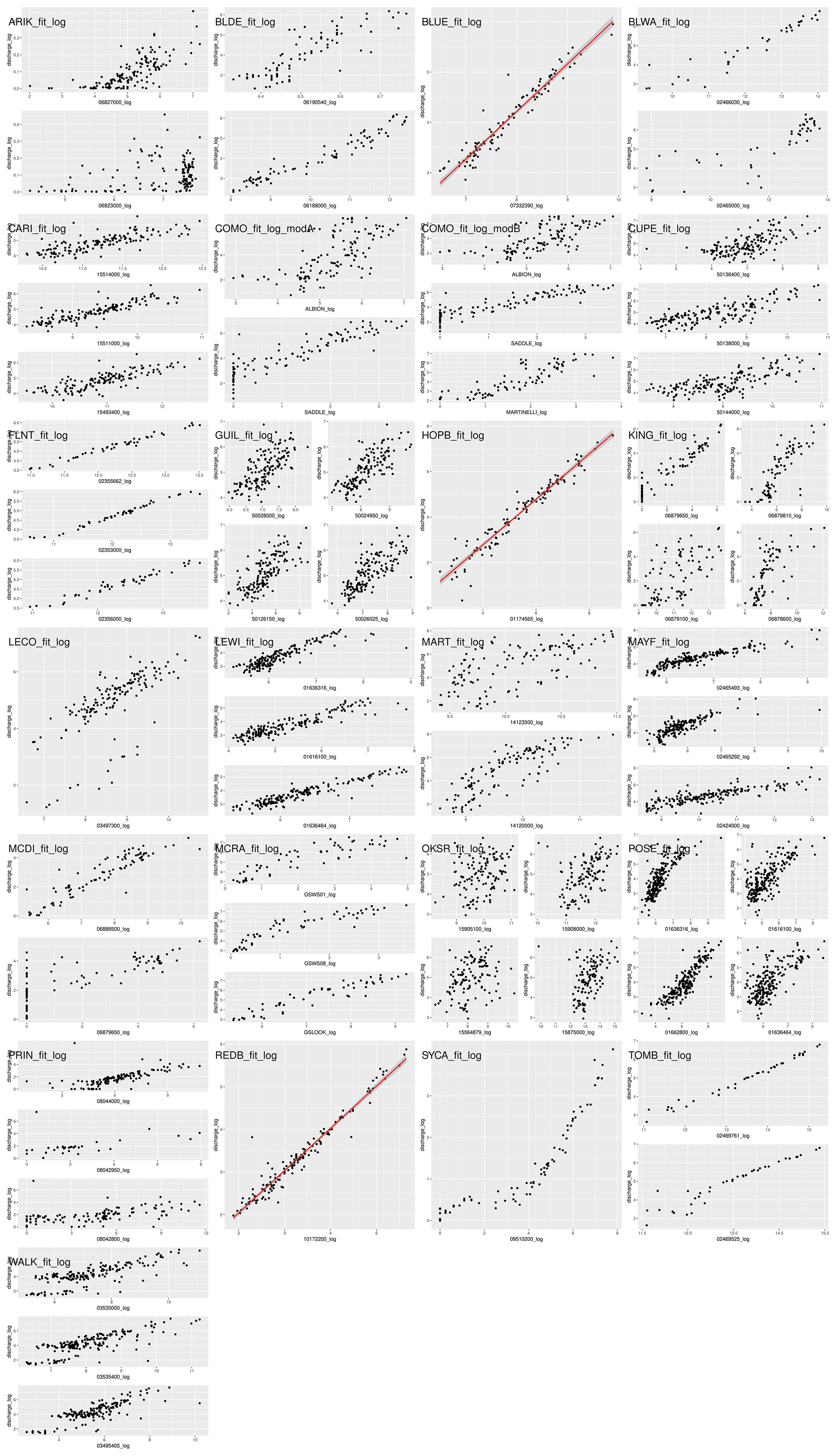
Figure A4 Marginal relationships between donor and target gauges for regression on specific discharge. Regression lines are shown only for single-donor regressions fitted via OLS. Site SYCA, here exhibiting a breakpoint, was modeled with segmented regression, and thus the regression line shown has no relevance.

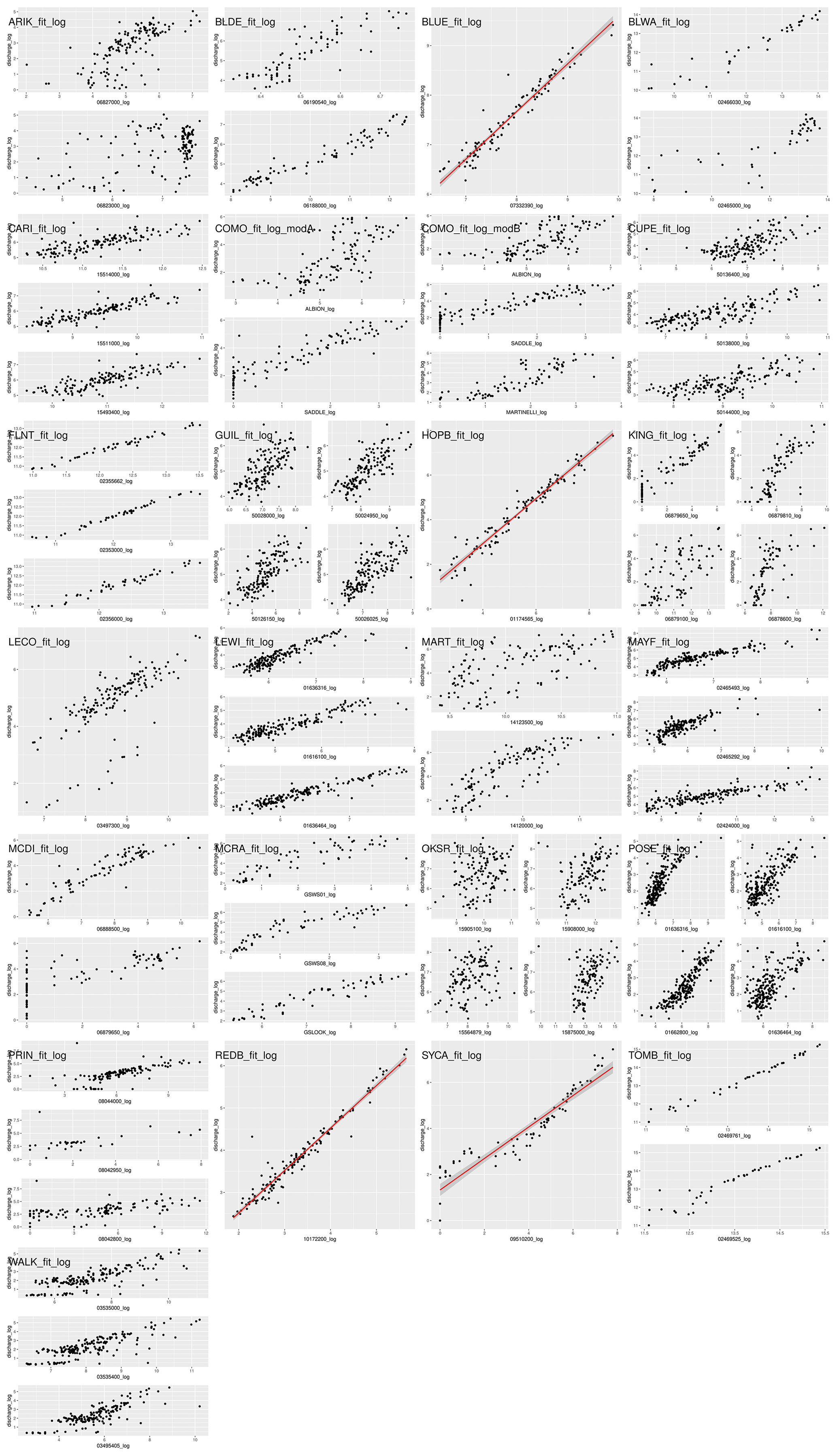
Figure A5 Marginal relationships between donor and target gauges for regression on absolute discharge. Regression lines are shown only for single-donor regressions fitted via OLS. Site SYCA, here exhibiting a breakpoint, could not be fitted via segmented regression in the context of absolute discharge.

Figure A6 Observed (field) discharge vs. ensembled LSTM predictions.

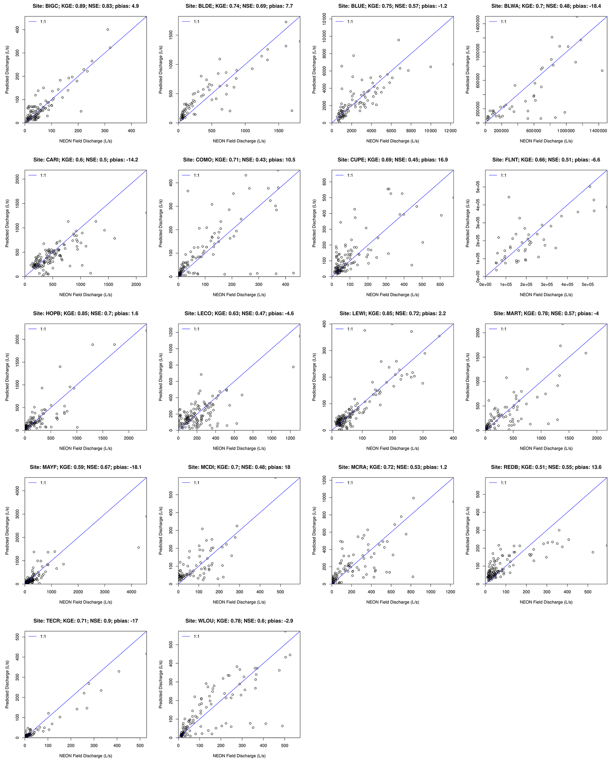
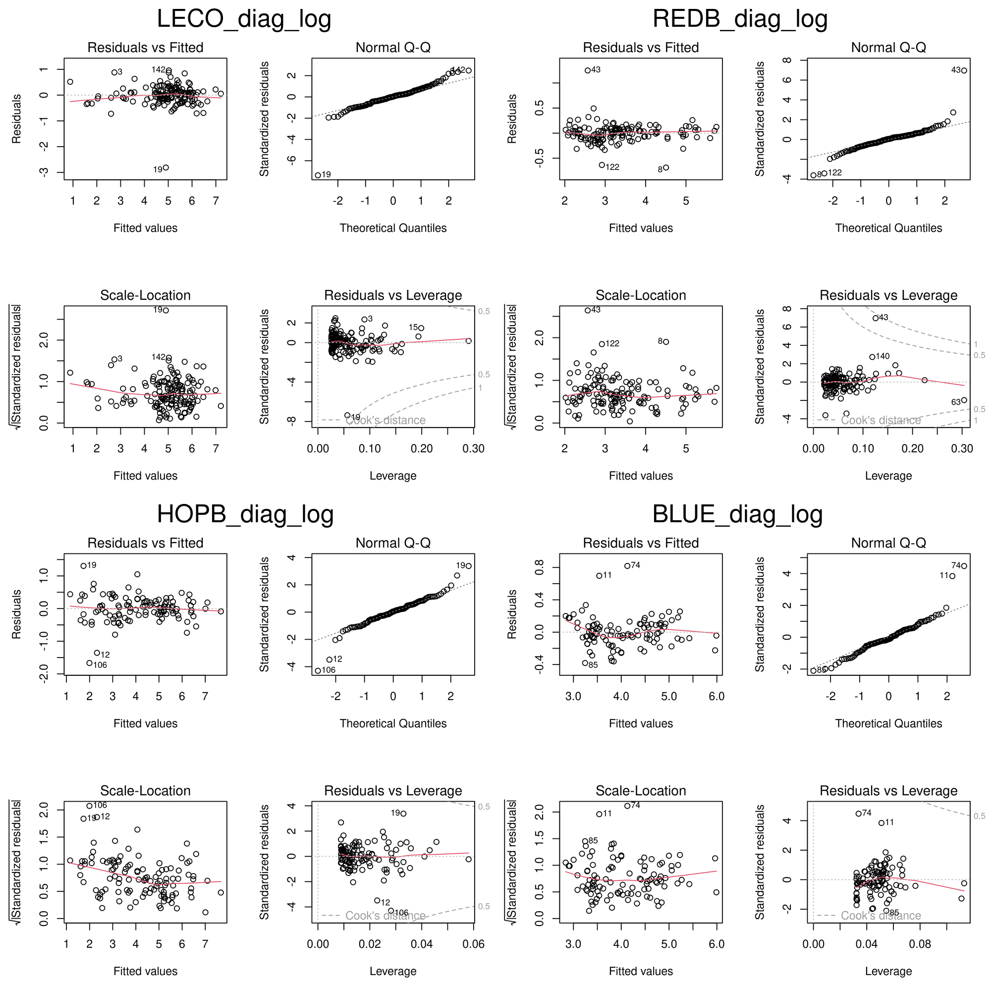
Figure A7 Diagnostic plots for the four sites modeled by OLS regression on specific discharge.

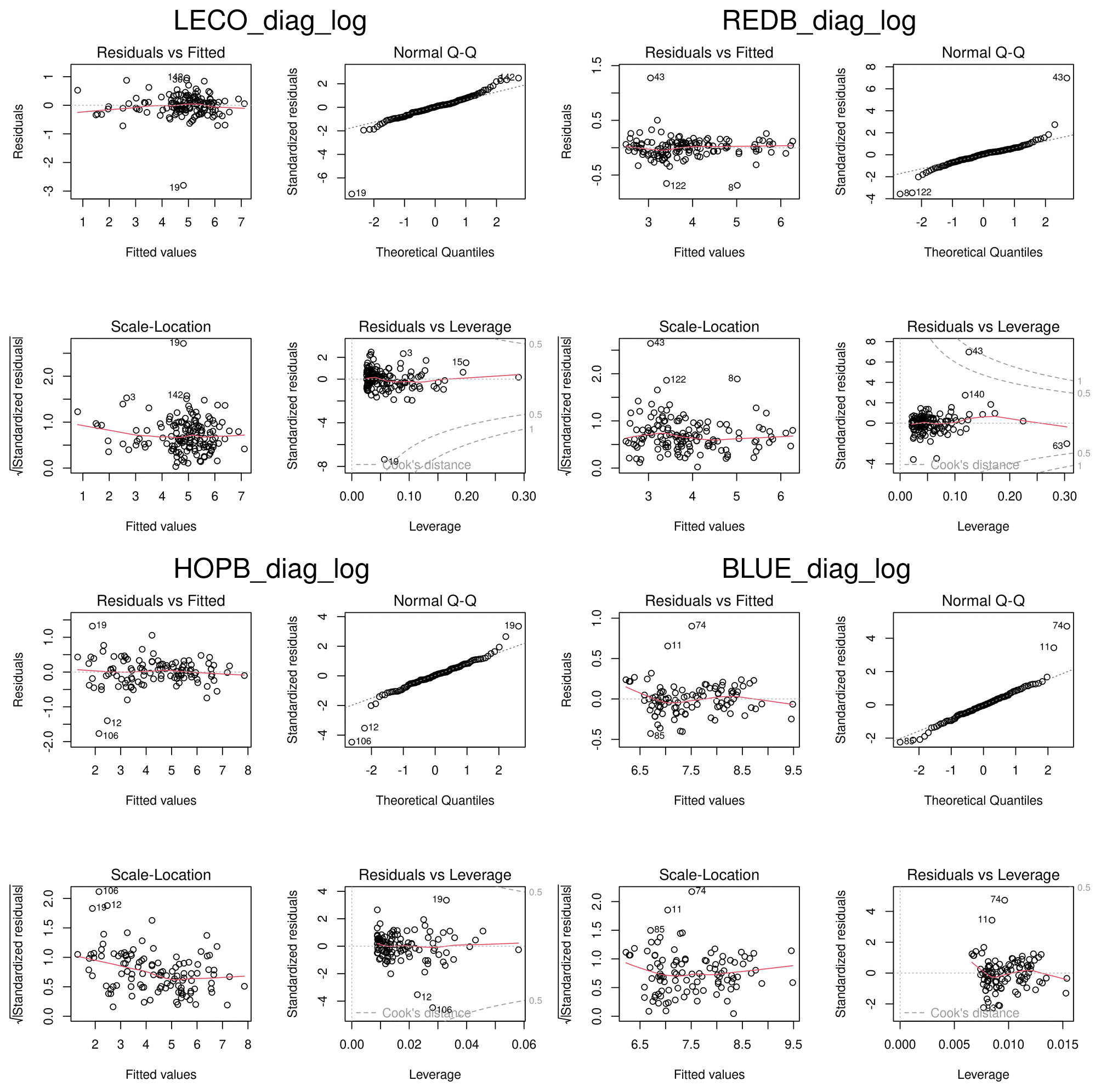
Figure A8 Diagnostic plots for the four sites modeled by OLS regression on absolute discharge.

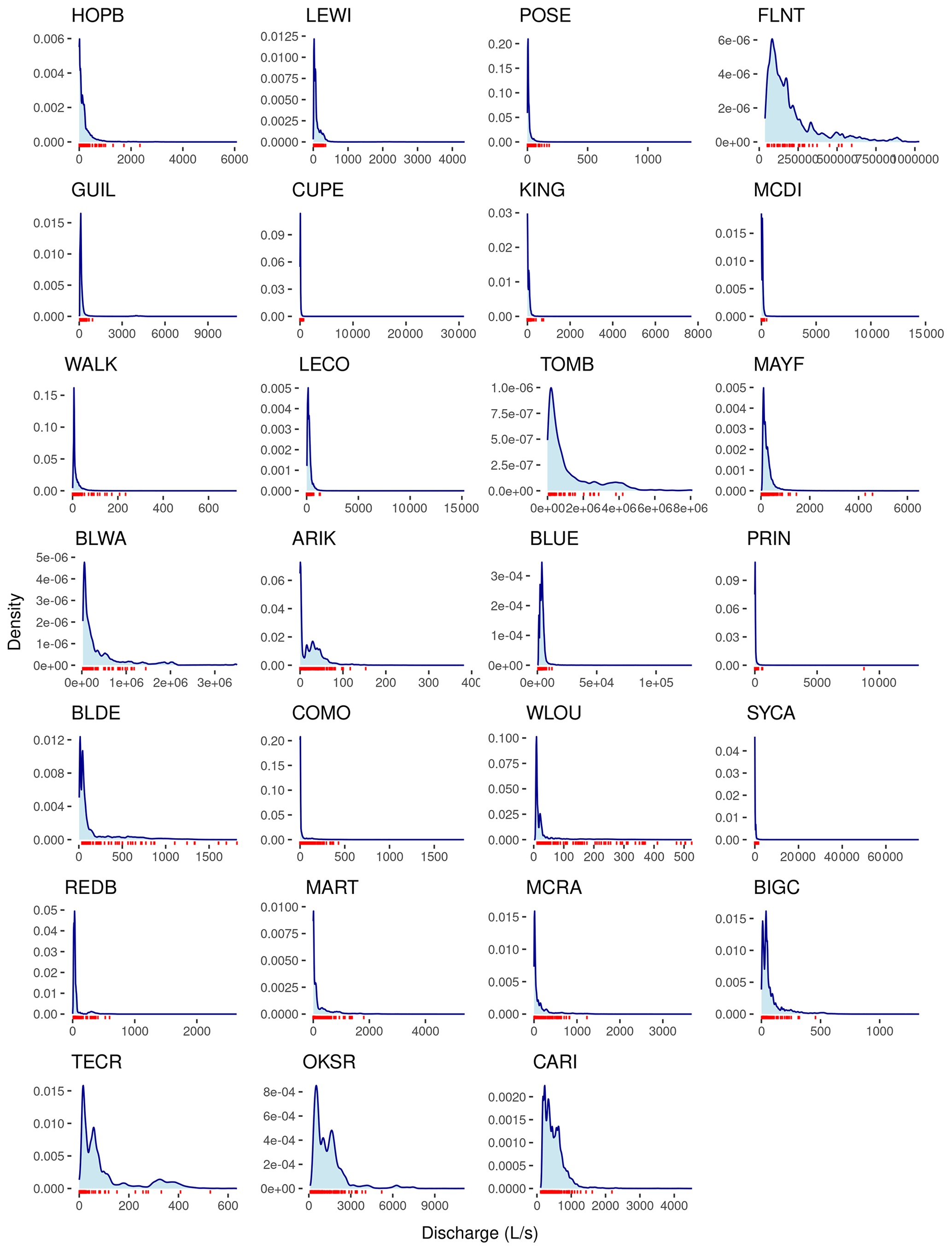
Figure A9 Density of NEON-estimated discharge (blue) relative to field-measured discharge observations (red marks).

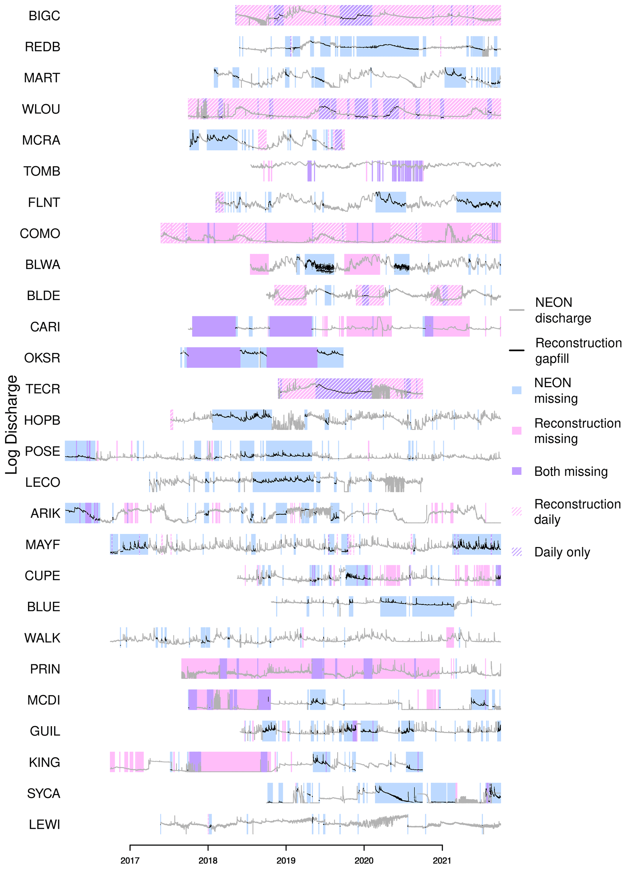
Figure A10 Durations of missing values (gaps) in NEON's 2023 release of continuous discharge time series, illustrating gaps filled or informed by estimates from this analysis. All officially published values are shown, including those with quality control flags. Sites are ordered as in Fig. 2. Gaps smaller than 6 h are not indicated.