HESS Opinions: Never train a Long Short-Term Memory (LSTM) network on a single basin

Machine learning (ML) has played an increasing role in the hydrological sciences. In particular, Long Short-Term Memory (LSTM) networks are popular for rainfall–runoff modeling. A large majority of studies that use this type of model do not follow best practices, and there is one mistake in particular that is common: training deep learning models on small, homogeneous data sets, typically data from only a single hydrological basin. In this position paper, we show that LSTM rainfall–runoff models are best when trained with data from a large number of basins.

1 Machine learning requires different intuitions about hydrological modeling

Regionalizing rainfall–runoff models across multiple watersheds is a long-standing problem in the hydrological sciences (Guo et al., 2021). The most accurate streamflow predictions from conceptual and process-based hydrological models generally require calibration to data records in individual watersheds. Hydrology models based on machine learning (ML) are different – ML models work best when trained on data from many watersheds (Nearing et al., 2021). In fact, this is one of the main benefits of ML-based streamflow modeling.

Because ML models are trained with data from multiple watersheds, they are able to learn hydrologically diverse rainfall–runoff responses (Kratzert et al., 2019b) in a way that is useful for prediction in ungauged basins (Kratzert et al., 2019a). However, prediction in ungauged basins is not the only reason to train ML models on data from multiple watersheds. Models trained this way have better skill even in individual, gauged watersheds with long training data records, and they are also better at predicting extreme events (Frame et al., 2022).

The purpose of this paper is to effect a change in intuition. ML requires a top-down modeling approach in contrast to traditional hydrological modeling that is usually most effective with a bottom-up approach. We do not mean top-down vs. bottom-up in the sense discussed by Hrachowitz and Clark (2017), who use these terms to differentiate between lumped, conceptual (top-down) vs. distributed, process-based (bottom-up) models. Instead, we mean that traditional hydrology models (both lumped, conceptual models and process-based models) are typically developed, calibrated, and evaluated at a local scale, ideally using long and comprehensive data records. Then, in this bottom-up approach, after a model is developed, we might work on regionalization strategies to extrapolate parameters and parameterizations to larger areas (e.g., Samaniego et al., 2010; Beck et al., 2016). In contrast, with ML modeling, the best approach is to start by training on all available data from as many watersheds as possible and then start fine-tuning models for individual catchments. The effort then goes into localizing large-scale models instead of regionalizing small-scale models.

This paper focuses on rainfall–runoff modeling with Long Short-Term Memory (LSTM) networks because this is currently the most common type of ML model used in surface hydrology. The use of LSTM networks for rainfall–runoff modeling is motivated by the fact that LSTM networks are state–space models and are therefore structured similarly to how hydrologists conceptualize watersheds (Kratzert et al., 2018). The use of LSTM networks in hydrology research has increased exponentially in the last several years (see Fig. 1). We see no reason to suspect that the lessons learned about big data with this type of model are not general, and we have several reasons to suspect that they are; namely, it is important to recognize that, across application domains, machine learning models trained on large training data sets out-perform smaller, more specialized models (Sutton, 2019).

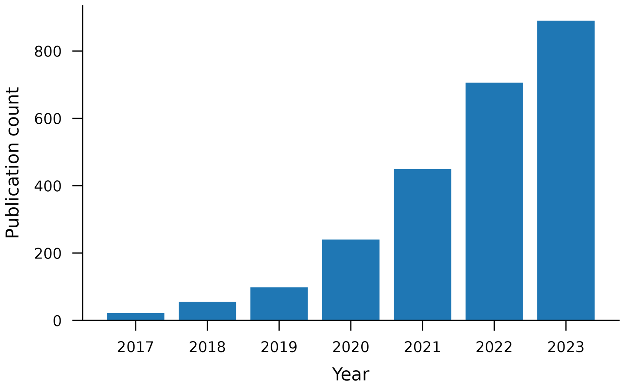
Figure 1 Number of hydrological publications related to rainfall–runoff modeling with LSTM networks over time based on data retrieved from Google Scholar in April 2024.

To understand the current state of practice with LSTM-based rainfall–runoff modeling, we collected papers returned by a keyword search on Google Scholar for “rainfall–runoff modeling LSTM streamflow”, sorted by relevance. From this search, we surveyed the top 50 papers per year for the years 2021, 2022, and 2023 and skipped papers that did not involve training models or developing systems for training models. Of those 150 papers surveyed, 122 trained models on individual catchments, and 28 trained models on multiple catchments (of which 4 were co-authored by one or more authors of this paper) (Fig. 2). We collected these 150 papers for review in April 2024, more than 4 years after the original regional LSTM rainfall–runoff modeling papers (Kratzert et al., 2019a, b) had been published. The list of 150 papers is included in the data repository released with this paper.

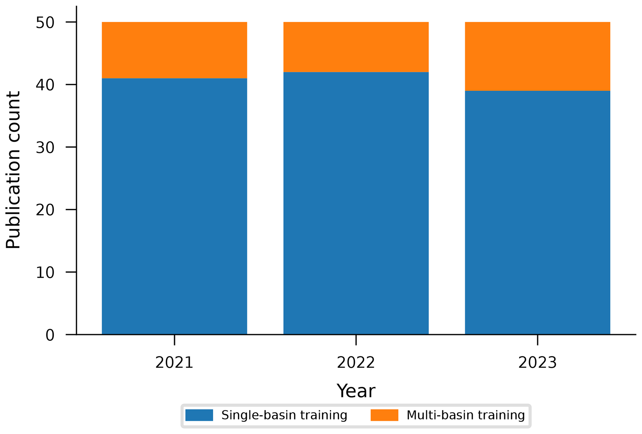
Figure 2 Fractions of 50 peer-reviewed research article papers per year (starting 1 year after the original LSTM regional-modeling papers were published Kratzert et al., 2019a, b) that train LSTM rainfall–runoff models on single vs. multiple basins, based on articles retrieved from Google Scholar in April 2024.

It is important to recognize that there is usually no reason in practice to train LSTM streamflow models using data from only a small number of watersheds. There is enough publicly available streamflow data to train robust ML models – for example, the various CAMELS data sets such as CAMELS-US (Newman et al., 2015), the Global Runoff Data Center (BAFG, 2024), or the Caravan data set and its extensions (Kratzert et al., 2023). It is possible to fine-tune large–sample models to individual locations and/or for specific purposes (e.g., Ma et al., 2021); however fine-tuning is outside the scope of this paper. It is sufficient for our purpose to show that training large-scale ML models is better than training small-scale ML models for streamflow prediction and that fine-tuning would only widen this difference.

In summary, the large majority of LSTM papers published in hydrology journals train models on small data sets from single catchments. This is unfortunate because it does not leverage the primary benefit of machine learning, which is the ability to learn and generalize from large data sets. The rest of this paper illustrates how and why that is a problem when using LSTM networks specifically for rainfall–runoff modeling.

2 Skill gaps between local and regional models

Figure 3 shows differences in performance between models trained on single basins vs. multiple basins (regional). Figure 3a shows this comparison for two traditional hydrology models, and Fig. 3b shows the comparison for LSTM models. Notice that, in Fig. 3a, single-basin models perform better than regional models, and in Fig. 3b, this is reversed.

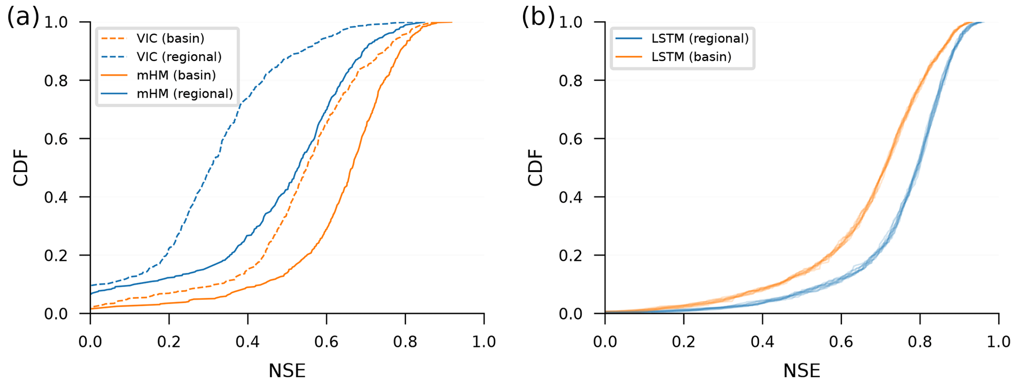
Figure 3 Cumulative density functions (CDFs) of Nash–Sutcliffe efficiencies (NSEs) of simulated volumetric discharge over watersheds in the CAMELS data set for models trained on individual basins (basin – orange lines) vs. on multiple basins (regional – blue lines). Subplot (a) shows a conceptual model (mHM) and a process-based model (VIC), both calibrated using data from 489 watersheds by (different) research groups that are familiar with each model – VIC single basins: Newman et al. (2017), VIC regional: Mizukami et al. (2017), mHM single basins: Mizukami et al. (2019), and mHM regional: Rakovec et al. (2019). Subplot (b) shows the same NSE CDFs from LSTM networks trained in two ways: regional LSTM networks (blue) were trained using data over the training period from all 531 CAMELS basins, and single-basin LSTM networks (orange) were trained using data over the training period from each CAMELS basin individually. An ensemble of 10 LSTM models were trained in all cases, where randomness in the LSTM repetitions is due to randomness in the initial weights prior to training. We recommend averaging hydrographs from this kind of repetition, as was done by Kratzert et al. (2019a, b).

Figure 3a shows cumulative density functions (CDFs) over Nash–Sutcliffe efficiencies (NSEs) for 489 CAMELS basins from a conceptual model (mHM) and a process-based model (VIC). These models were calibrated and run by other research groups without our involvement, and the data from these models were borrowed from the benchmarking study by Kratzert et al. (2019b). The fact that conceptual and process-based hydrological models perform worse when regionally calibrated is, to our knowledge, a consistent finding across hydrological-modeling studies (e.g., Beck et al., 2016; Mizukami et al., 2017).

Figure 3b shows the same NSE CDFs for LSTM models. We tuned the hyperparameters and trained an ensemble of 10 single-basin LSTM models separately for each of the 531 basins in the CAMELS data set (Newman et al., 2015; Addor et al., 2017) using a standard training–validation–test data split, with approximately 10 years of data in each split. We similarly trained an ensemble of 10 LSTM regional models with data from all 531 CAMELS catchments simultaneously using hyperparameters taken from Kratzert et al. (2021). Details about how LSTM models were hyper-tuned, trained, and tested can be found in Appendix A.

The choice to use 531 CAMELS basins for training and testing LSTM networks comes from the suggestion by Newman et al. (2017), who selected these basins from the full CAMELS data set for model benchmarking. We use this set of CAMELS benchmark gauges for the remainder of this study. Figure B1 shows the same comparison as Fig. 3, but subpanel b in that figure shows NSE CDFs only for the 489 CAMELS basins with mHM and VIC runs.

The takeaway from Fig. 3 is that, whereas traditional hydrological models are more accurate when calibrated to a single watershed, LSTM models are more accurate when trained on data from many watersheds. Other hydrological metrics are reported in Appendix E; however, the main point of our argument holds regardless of which metric is used for evaluation.

3 Why this matters for extreme events

Training on large-sample data sets with hydrologic diversity means that the training envelope is larger, making it less likely that any new prediction will be an extrapolation. Intuitively, the training envelope refers to the ranges of data where model performance is well-supported by the training process. If the training set includes a very humid basin then the model is more likely to have seen large precipitation events so that a new extreme precipitation event seen during inference is less likely to be outside of the training envelope. As an example of this, Nearing et al. (2019) discussed how watersheds can move within the training envelope as (e.g., climate) conditions within a catchment change and how this causes changes in the modeled rainfall–runoff response in individual watersheds.

We can look at the target data to see an example of how this diversity in training data helps. The LSTM models used by Kratzert et al. (2019a) and Kratzert et al. (2019b) have a linear “head” layer that produces a scalar estimate of streamflow at each time step by taking a weighted sum of the values of the LSTM hidden state. The weights for this weighted sum in the head layer are parameters that are tuned during training. The LSTM hidden state is a real-valued vector in (−1, 1) and has a size equal to the number of cell states or memory states in the LSTM model (for a hydrologically centered overview of the structure of an LSTM model, please see Kratzert et al., 2018), which means that the maximum (limiting) value of the scalar streamflow estimate from the model is defined by the sum of the absolute values of weights in the head layer (see also Appendix C). More diversity in training data (here, training targets) causes the model to expand the range of weights in the head layer to accommodate higher flow values.

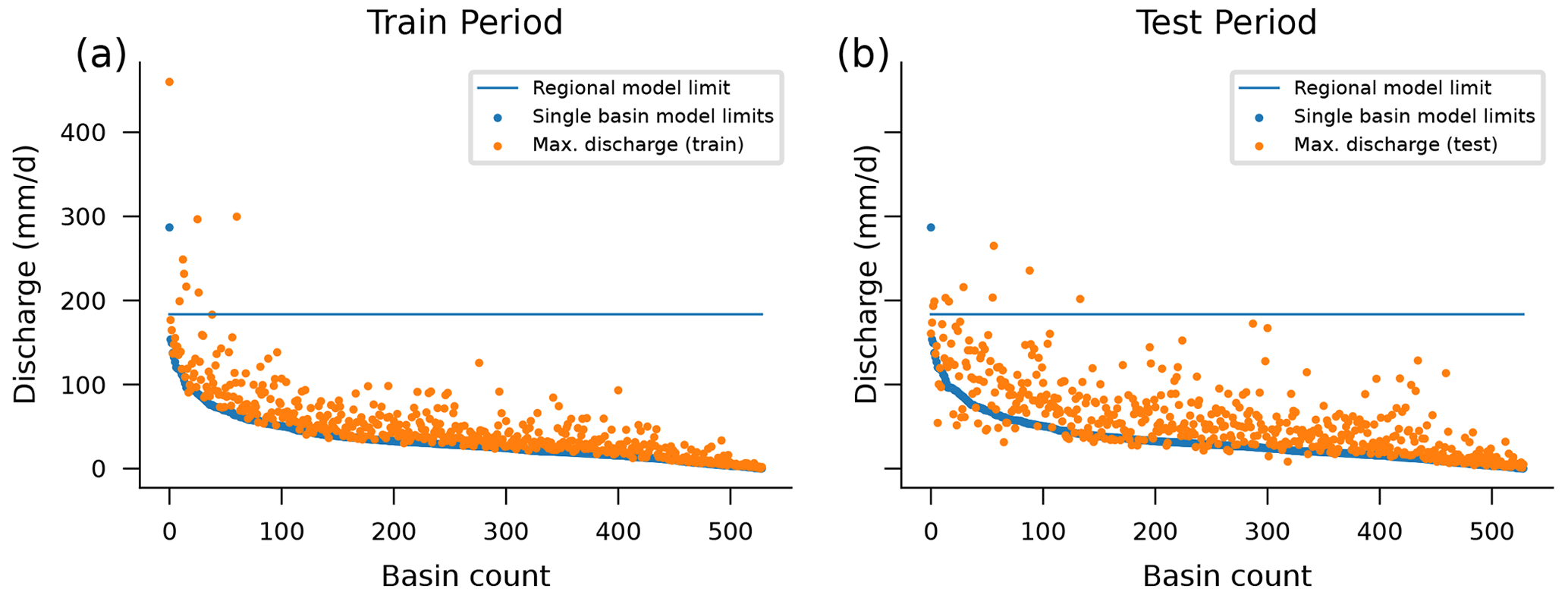
Figure 4 Theoretical maximum streamflow prediction of an LSTM model with a linear head layer when trained per basin (blue dots) and for all 531 CAMELS basins together (blue line). Orange dots represent the maximum streamflow values per basin in the training period (a) and test period (b). In the test period, there are 10 flow values above the maximum prediction of the regional model, while there are more than 6346 flow values above the theoretical maximums of their respective single-basin models across all basins.

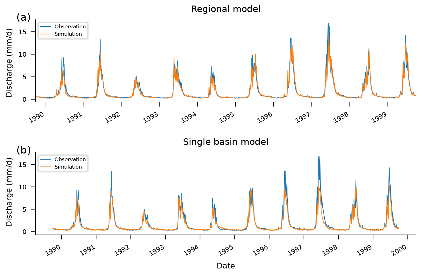
Figure 5 Observed and simulated hydrographs from the test period (1989–1999) in a particular basin (13011900). Notice how the high-flow effect outlined in Fig. 4 manifests in the differences between hydrographs predicted by a regional LSTM model (a) vs. a single-basin LSTM model (b). This example was chosen to highlight this effect (not chosen randomly); however, the effect is similar in most basins. This gauge is on Lava Creek in Wyoming, with a drainage area of 837 km², and exhibits a strong seasonal flow pattern.

This effect can be seen in Fig. 4, which shows the theoretical maximum prediction from each of the 531 single-basin LSTM models and from a single LSTM model trained on all 531 CAMELS basins. During inference (test period), there is a total of 10 streamflow observations across all 531 catchments that are above the regional model's theoretical maximum when trained on data from all 531 watersheds. However, when separate models are trained per catchment, there are more than 6000 streamflow observations that are above the theoretical maximums for each model in its respective catchment. Figure 5 shows how this effect manifests in an example hydrograph from one particular basin (not chosen at random). More examples are given in Appendix D. Notice that no model captures all of the extreme events, even in the training data set (which is common for physically based models as well; Frame et al., 2022).

In summary, training on a larger data set means that the model is able to adapt internal weights and biases to account for more extreme events.

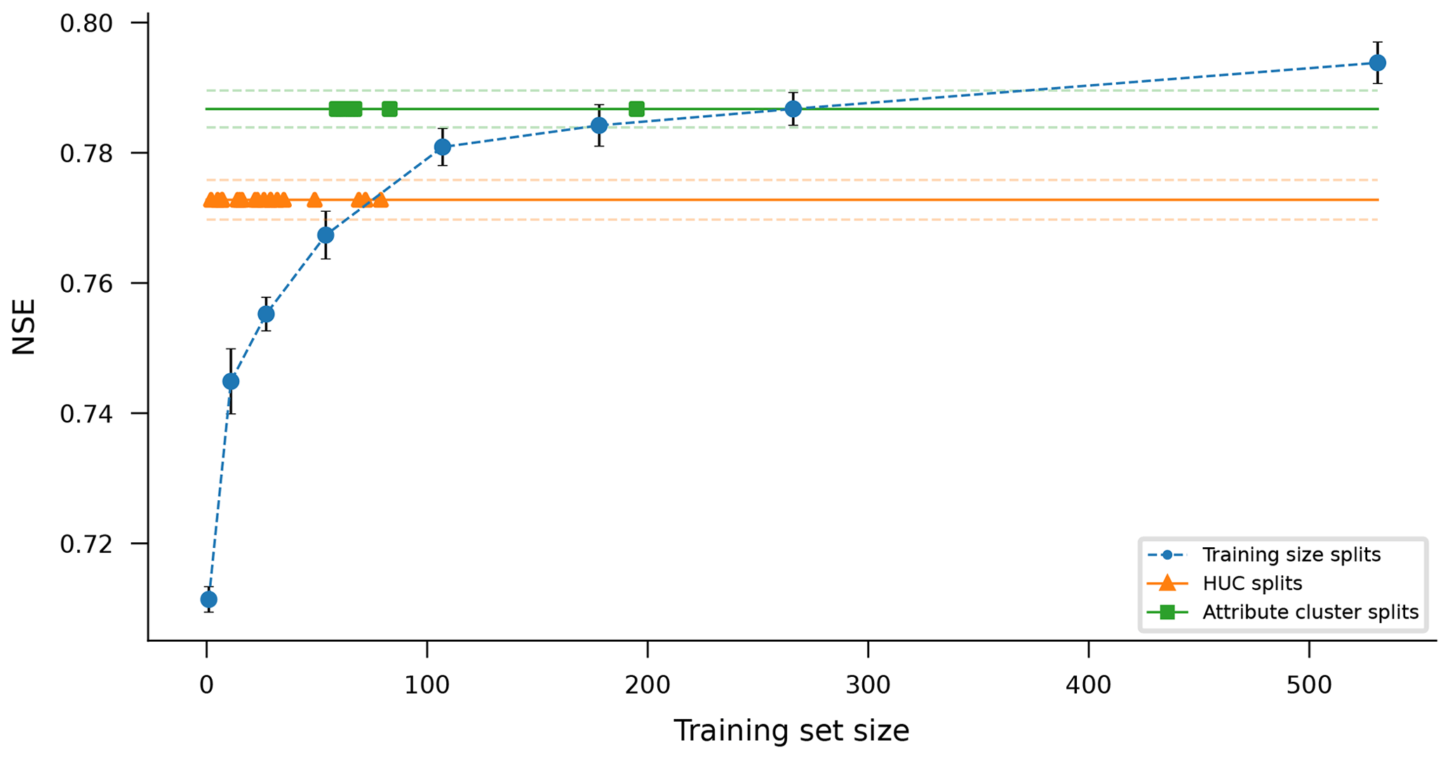
Figure 6 Median NSE scores of simulated volumetric discharge over 531 CAMELS basins for LSTM models trained and tested on splitting the 531 CAMELS basins into different groupings for training and testing. All models were tested on the same basins where they were trained (during different time periods). The blue line represents basin groupings of different sizes chosen randomly without replacement so that all 531 basins were modeled exactly once for each grouping size. Orange and green lines show results from grouping the 531 basins into sets based on USGS hydrological unit codes (orange) and k-means clustering of basin attributes (green). Dots on the orange and green lines indicate the sizes of the (18 and 6) basin groups used in those splits since there are a different number of CAMELS basins in each HUC and a different number of basins in each attribute cluster. Blue dots and solid orange and green lines represent the median model performance over 531 basins, while blue error bars and dashed orange and green lines represent the standard deviation of this median over a 10-member ensemble.

4 How many basins are necessary?

Figure 6 shows how test period performance increases as more basins are added to the training set. The blue line in this figure was created by grouping 531 CAMELS basins into differently sized training and test groups randomly without replacement. This was done using k-fold cross-validation so that all models were tested on the same basin(s) where they were trained (during different time periods) and so that every basin was used as a test basin exactly once in each grouping size. For example, the 531 basins were grouped into, e.g., five disjointed groups (each with around 107 basins), following which the data from the training period (1999–2000) of one group were used to train an ensemble of 10 LSTM models, and data from the test period (1980–1989) of the same group were used to evaluate that ensemble of trained LSTM models. This procedure was repeated for each of the remaining four groups, and a similar procedure was used for each different size of basin grouping, shown along the x axis of Fig. 6. Figure 6 plots the average (over 10 ensemble members) of the median (over 531 CAMELS basins) test period NSE for various basin groupings. More details about basin groupings can be found in Appendix A3.

The blue line in Fig. 6 shows performance (median NSE) increasing as the size of the training data set increases. This effect continues up to the maximum size of the CAMELS data set (531 basins). In other words, it is better to have more basins in the training set, and even these 531 basins are most likely not to be enough to train optimal LSTM models for streamflow.

5 Is hydrological diversity always an asset?

There are at least two factors to consider when choosing training data: volume and variety. Volume refers to the total number of data used for training (more is always better, as far as we have seen), and variety refers to the (hydrologic) diversity of data. Diversity might be in the form of different geophysical catchment attributes, different types and magnitudes of events, or different hydrological behaviors.

Figure 6 provides examples of training on less hydrologically diverse basin groups. The orange line in Fig. 6 shows the mean (over 10 ensemble members) of the median NSE (over 531 CAMELS basins) from training and testing models on basins grouped by USGS hydrological unit codes (HUCs). There are 18 HUCs represented in the CAMELS data set, with between 2 and 79 basins per HUC. The green line in Fig. 6 shows the mean (over 10 ensemble members) of the median NSE (over 531 CAMELS basins) from training and testing models on basin groups derived from k-means clustering on static catchment attributes. The CAMELS data set includes catchment attributes related to climate, vegetation, pedology, geology, and topography, and we clustered using 25 catchment attributes, described in Table A1. We selected a k-means clustering model based on a maximin criterion based on silhouette scores, which resulted in a model with six clusters ranging from 59 to 195 basins per cluster. Details about how models were trained and tested on HUCs and attribute clusters can be found in Appendices A4 and A5.

Figure 6 provides evidence that there might be ways to construct training sets that could potentially result in better models than simply training on all available streamflow data. This conclusion is hypothetical because in all the examples shown in Fig. 6, models trained on any subset of the 531 CAMELS basins performed worse, on average, than models trained on all 531 CAMELS basins. However, separating the training set into hydrologically similar groups of basins results in models that perform better than models trained on random basin groups of similar size. It is an open question as to whether a larger data set than CAMELS (e.g., Kratzert et al., 2023) might be divisible into hydrologically similar groups that individually perform better than a model trained on all available data. This could happen if, for example, the curve in Fig. 6 becomes asymptotic at some point beyond the size of the CAMELS data set and if the performance of models trained on hydrologically informed basin groups continues to increase with sample size. Note that this analysis does not account for the value of hydrologic diversity for prediction in ungauged basins.

The takeaway is that, even if enough basins exist to divide your training data into hydrologically informed training sets, one is likely to be better off simply training a single model with all available data. At least, one should perform an analysis like that which is shown in Fig. 6 to understand whether splitting the training set helps or hurts. We are interested in seeing (through future work) what these trade-offs look like with larger training sets.

6 Are bigger models better everywhere?

Even though the best model, on average, is the model trained on all 531 CAMELS basins, it is not the case that the model trained on all 531 CAMELS basins is better in every basin. Figure 7 shows the number of basins for which models trained on each grouping (size, HUC, attributes cluster) perform statistically better than (green) – and not statistically differently to (orange) or statistically worse than (blue) – the regional model trained on all 531 basins. These statistical tests were done using a two-sided Wilcoxon signed-rank test over 10 repetitions of each model, with a significance level of α=0.05. All models perform worse than the full regional model in more basins than they perform better in.

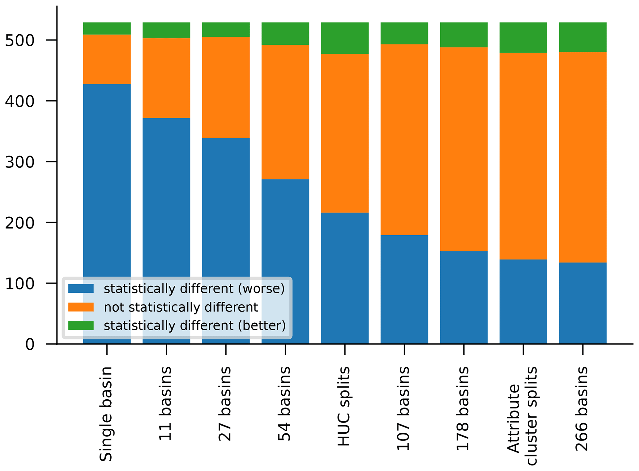
Figure 7 Counts of basins for which models trained on each grouping (sizes, HUC, attributes cluster) perform statistically better than (green) – and not statistically differently to (orange) or statistically worse than (blue) – the regional model trained on all 531 basins. Significance was assessed using a two-sided Wilcoxon signed-rank test over 10 repetitions of each model, with a significance level of α=0.05.

We have not found a way to (reliably) predict which model will perform best in any particular basin. It is not possible to use metrics from the training period or validation period to (reliably) choose the best model in the test period. Additionally, we have tried extensively to construct a separate predictor model that uses catchment attributes and/or hydrological signatures to predict whether one model will perform better or worse than other models in specific basins. We have not been able to construct a model that performs well at this task. Details of these predictability experiments are out of the scope of this paper, but a relevant example was given by Nearing et al. (2024).

7 Conclusion

The main point that we would like readers to take from this opinion paper is that training LSTM networks for rainfall–runoff modeling requires using data from many basins. We have seen a number of papers that train large ML models (LSTM models or similar) on very small data sets, and many of these papers then go on to test some type of adaptations that seem to offer improvement. Of course, it is trivial (but most likely uninteresting) to beat improperly trained models. It would be interesting to show that adding physics to a well-trained ML model adds information – so far, to our knowledge, all attempts to add physics to (properly trained) streamflow LSTM models in hydrology have produced lower-performing models.

Whatever goal a researcher might have for training an ML-based rainfall–runoff model, there is no reason not to train the model with a large-sample data set. There is enough publicly available streamflow data that there should never be an excuse not to use at least hundreds of basins for training. This is true even if the focus of a particular study is on one watershed or a small number of watersheds.

Appendix A: Hyperparameter tuning, training, and testing

All models in this paper were trained using data from the CAMELS data set (Newman et al., 2015; Addor et al., 2017). Building on the community benchmarking experiment proposed by Newman et al. (2017) and used by many LSTM modeling studies (e.g., Kratzert et al., 2019a, b, 2021; Frame et al., 2021, 2022; Klotz et al., 2022; Nearing et al., 2022), we trained and tested models on 531 CAMELS basins using time periods for training (1 October 1999 through 30 September 2008), validation (1 October 1980 through 30 September 1989), and testing (1 October 1989 through 30 September 1999). All models were trained and evaluated using NeuralHydrology v.1.3.0 (Kratzert et al., 2022) with an NSE loss function. All LSTM models consist of a single-layer LSTM with a linear head layer.

A1 Regional LSTM model

The regional LSTM model uses hyperparameters from Kratzert et al. (2021). The most important hyperparameters are as follows: hidden size (256), dropout (40 % dropout in the linear output layer), optimizer (Adam), number of epochs (30), learning rate (initial learning rate $\mathrm{1}\times {\mathrm{10}}^{-\mathrm{3}}$, reduced to $\mathrm{5}\times {\mathrm{10}}^{-\mathrm{4}}$ at epoch 20 and further reduced to $\mathrm{1}\times {\mathrm{10}}^{-\mathrm{4}}$ at epoch 25), sequence length (365), and loss function (adapted NSE loss; see Kratzert et al. (2019b)).

After training, we picked the weights from the epoch with the highest validation metric (median NSE across all basins) and evaluated the model with these weights on test period data from all 531 CAMELS catchments. Validation curves for all 10 regional models over 30 training epochs are shown in Fig. A1.

A2 Single-basin LSTM models

Single-basin LSTM models were trained for each basin individually and used the same basic architecture as described in Sect. A1: a single-layer LSTM followed by a linear head layer. Hyperparameters were tuned specifically for each basin for the experiments in this paper using the two-step procedure outlined below. Both steps were done with a grid search.

First step. We used three repetitions of each hyperparameter setting for each basin (n=531) with different random seeds for initializing the weights. All models were run for 100 epochs using the Adam optimizer with a learning rate of $\mathrm{5}\times {\mathrm{10}}^{-\mathrm{3}}$ and a batch size of 256. During training, the model was validated after every four epochs on validation period data. Hyperparameters were chosen using the model settings with the highest median NSE scores over the three repetitions in any validation epoch (hidden size: (8, 16, 32); dropout rate on the head layer: (0.0, 0.2, 0.4, 0.5)).

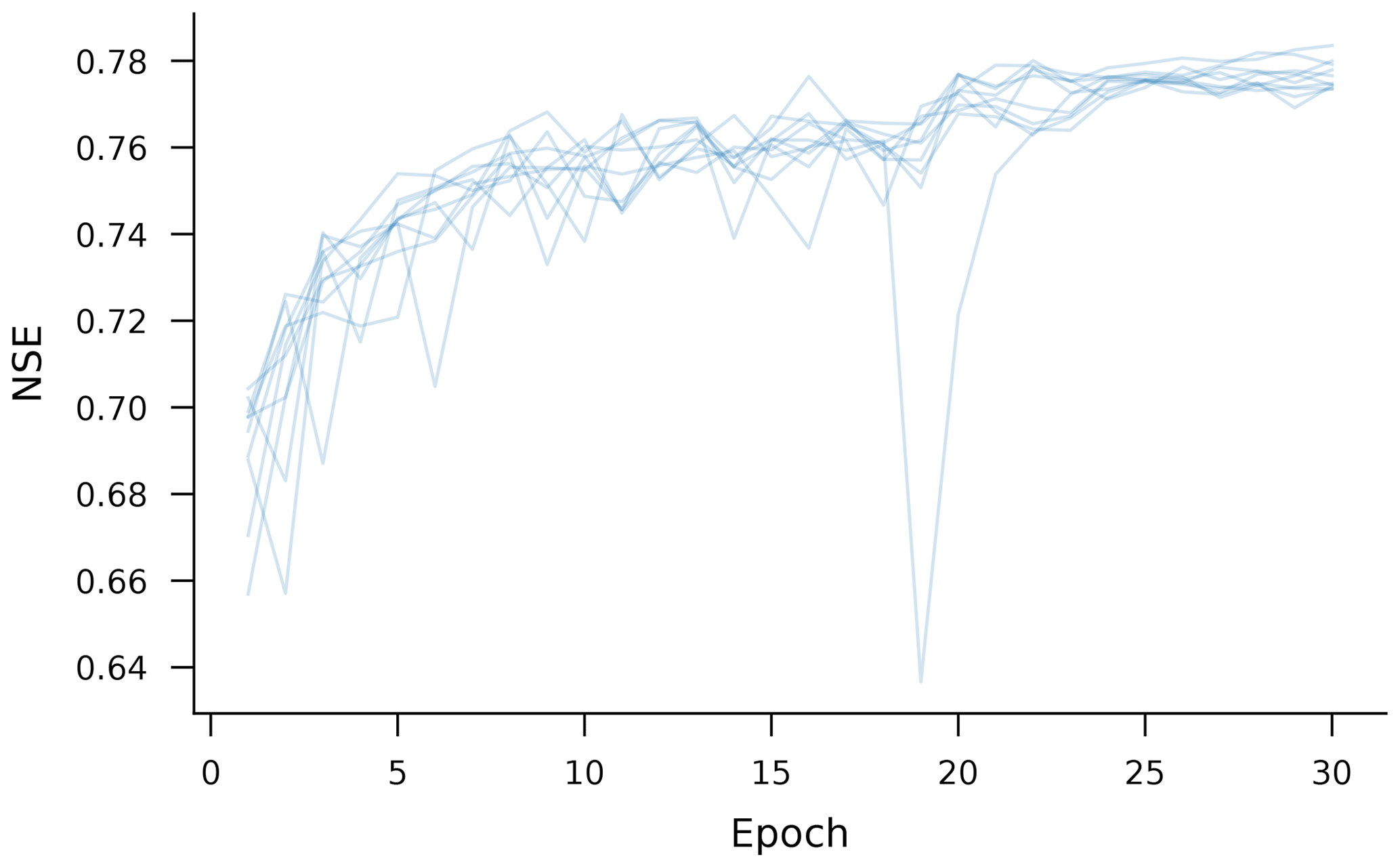
Figure A1 Validation scores of all 10 repetitions of the regional model over training epochs.

For all models, we used the same sequence length (n=365) as for the regional model.

Second step. Using the hyperparameters chosen from the first step, we tuned the learning rate and batch size in a similar way, maximizing over the median NSE over three model repetitions: learning rate of ($\mathrm{5}\times {\mathrm{10}}^{-\mathrm{3}}$, $\mathrm{1}\times {\mathrm{10}}^{-\mathrm{3}}$, $\mathrm{5}\times {\mathrm{10}}^{-\mathrm{4}}$, $\mathrm{1}\times {\mathrm{10}}^{-\mathrm{4}}$) and batch size of (128, 256, 512).

For each basin, separately, we picked model weights from the best validation epoch of the model with the highest NSE score over all validation epochs from all models in each basin.

Final training and evaluation. Given the set of per-basin optimized parameters, we trained 10 models per basin, each with a distinct random seed. All statistics reported in this paper for all models are from test period data, except where otherwise noted.

A3 Random basin splits of different sizes

Models reported in Fig. 6 were tuned (hyperparameters chosen), trained, and tested in a way that is similar to the single-basin LSTM models described in Appendix A2. For random basin splits, we divided the 531 CAMELS basins into random sets without replacement using six different sizes of split that were chosen by (approximately) dividing the full 531-basin group into basin groups of [50, 20, 10, 5, 3, and 2]. An example of one of these random splits with five groups (approximately 107 basins per split) is shown in Fig. A2.

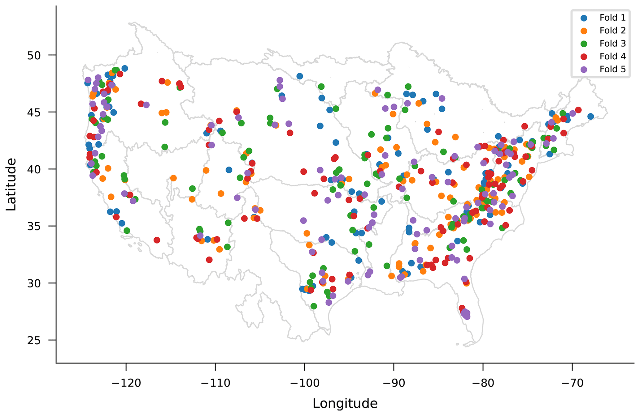
Figure A2 Basin location of random split with five groups of approximately 107 basins per group.

Choosing hyperparameters was done as described in Appendix A2, except that, for these splits, we did not use three random repetitions and only trained up to 30 epochs to reduce computational expense. We also expanded the hyperparameter search slightly due to our experience in training larger models – the hyperparameter ranges for the two grid search stages were as outlined below.

First step. This was characterized by a hidden size of (8, 16, 64, 128, 256) and a dropout rate on the head layer of (0.0, 0.2, 0.4, 0.5).

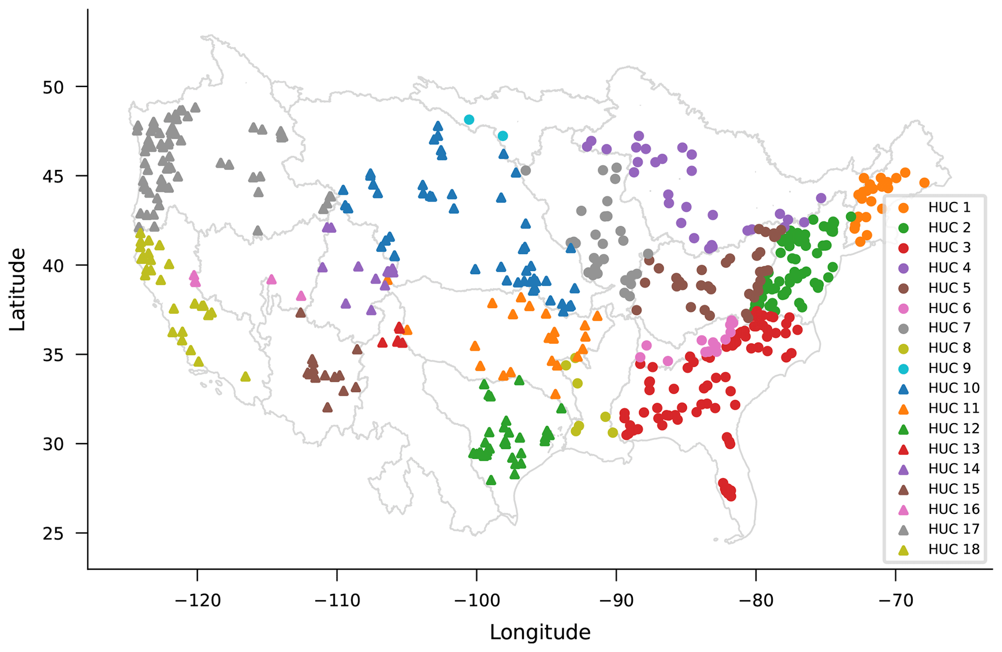
Figure A3 Spatial location of basins split by USGS hydrological unit code 02.

Second step. In the second stage, we always used a batch size of 256 (as with the regional model) and tuned over the following multi-stage learning rates, where the index is the epoch during which the learning rate switched to the listed value:

• 0: $\mathrm{5}\times {\mathrm{10}}^{-\mathrm{3}}$, 10: $\mathrm{1}\times {\mathrm{10}}^{-\mathrm{3}}$, 25: $\mathrm{5}\times {\mathrm{10}}^{-\mathrm{4}}$

• 0: $\mathrm{1}\times {\mathrm{10}}^{-\mathrm{3}}$, 10: $\mathrm{5}\times {\mathrm{10}}^{-\mathrm{4}}$, 25: $\mathrm{1}\times {\mathrm{10}}^{-\mathrm{4}}$

• 0: $\mathrm{5}\times {\mathrm{10}}^{-\mathrm{4}}$, 10: $\mathrm{1}\times {\mathrm{10}}^{-\mathrm{4}}$, 25: $\mathrm{5}\times {\mathrm{10}}^{-\mathrm{5}}$

• 0: $\mathrm{1}\times {\mathrm{10}}^{-\mathrm{4}}$, 10: $\mathrm{5}\times {\mathrm{10}}^{-\mathrm{5}}$, 25: $\mathrm{1}\times {\mathrm{10}}^{-\mathrm{5}}$.

A4 Hydrological-unit-code splits

The orange curve in Fig. 6 shows median NSE scores over CAMELS basins that result from LSTM models trained on basin groups defined by USGS HUCs. Figure A3 shows the locations of the 531 CAMELS basins by HUC region. The set of 531 basins was divided according to these geographical regions, and a separate model was trained on all basins from each. Hyperparameter tuning was done as described in Appendix A3. Testing was done as described in Appendix A2.

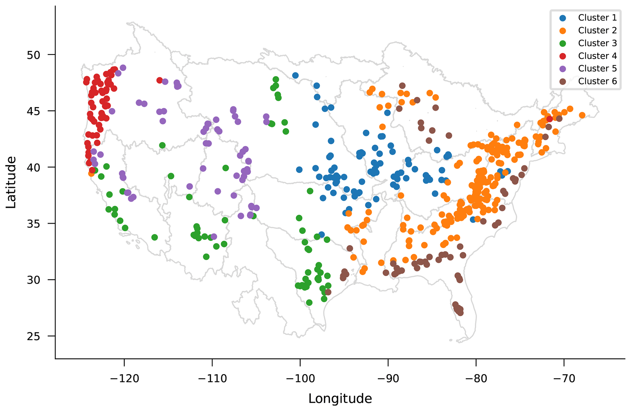
Figure A4 Spatial location of basins split by k-means clustering based on the basin attributes.

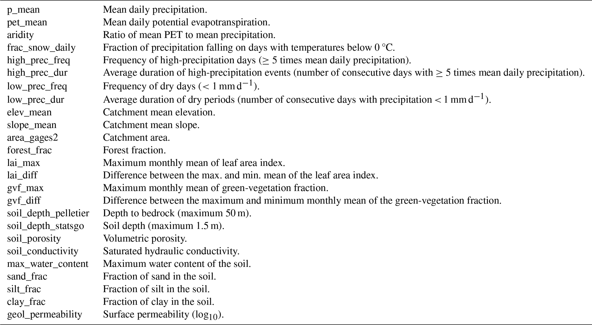
Table A1 Table of catchment attributes used in this experiment. Description taken from the data set of Addor et al. (2017).

A5 Attribute cluster splits

The green curve in Fig. 6 shows median NSE scores over CAMELS basins that result from LSTM models trained on basin groups defined by k-means clustering based on static catchment attributes. The catchment attributes used for clustering are described in Table A1. These are almost the same attributes that were used by Kratzert et al. (2019b) but without the carbonate-rock fraction and the seasonality of precipitation (the former is often zero, and the latter is categorical, both of which make clustering slightly more difficult).

We performed k-means clustering on these 25 basin attributes (all attributes were normalized) using 300 iterations and 10 random initializations. Using a maximin criterion based on silhouette scores for between 3 and 100 clusters, we chose to divide basins into six groups with sizes of 83, 195, 67, 61, 66, and 59 basins. These clusters are mapped in Fig. A4.

Appendix B: Regional vs. single-basin model comparison

Figure 3 illustrates a difference between how LSTM models and conceptual models behave when trained regionally vs. locally (on single basins). Specifically, the LSTM performs best when trained regionally, while traditional models perform best when trained locally.

Figure B1 illustrates the same comparison, but where the LSTM NSE CDFs in Fig. B1b only consider the same 489 CAMELS basins that are used in the mHM and VIC NSE CDFs in Fig. B1a. This is a more direct comparison than what is shown in Fig. 3; however, the results of the comparison are qualitatively identical.

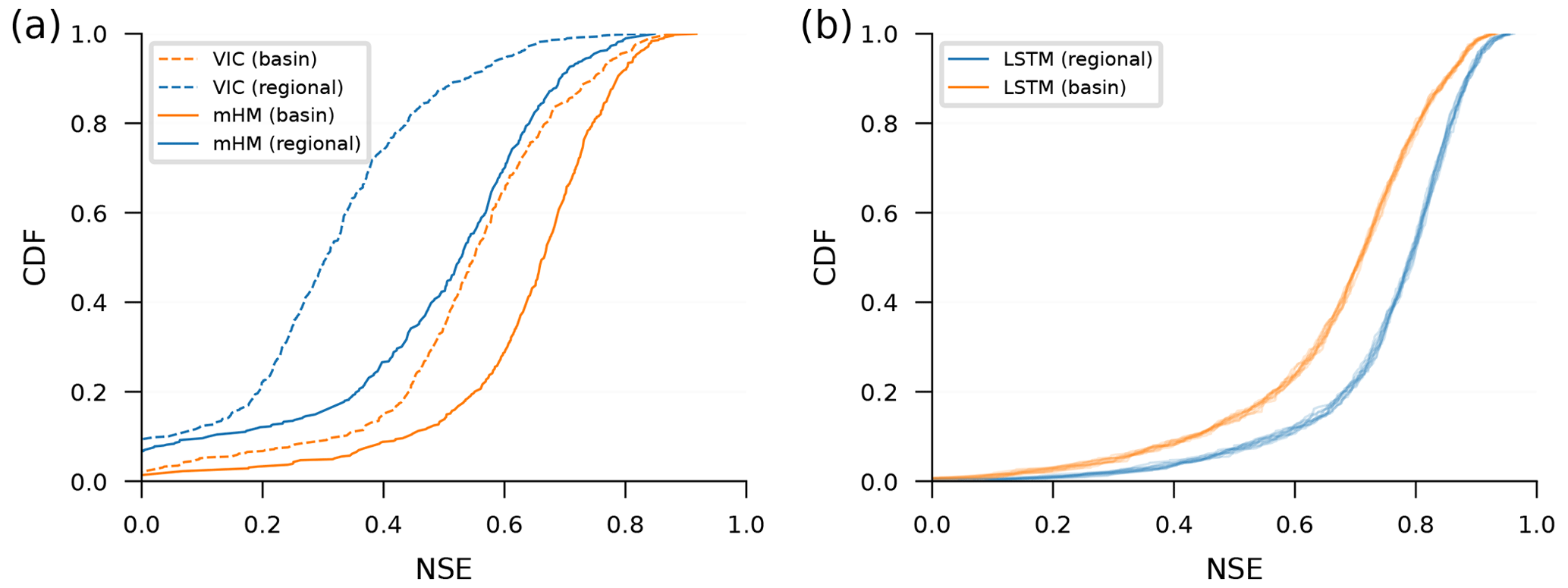
Figure B1 This figure is identical to Fig. 3 except that (b) uses all 531 CAMELS basins that Newman et al. (2017) recommended using for model benchmarking and which were used in all other experiments reported in this study.

Appendix C: Theoretical prediction limit

Figure 4 shows the theoretical maximum prediction limits for regional and single-basin LSTM models. To understand how those limits were derived, it is important to understand how the output of the LSTM layer is computed and how this output translates into the model prediction.

The output of the LSTM layer, h_t, is computed according to the following equation:

$$\begin{array}{}\text{(C1)}& h_t=o_t\odot \tanh \left(c_t\right),\end{array}$$

where o_t is the output gate at time step t, tanh( ) is the hyperbolic tangent function, and c_t is the LSTM cell state of time step t. The output gate is computed according to the following equation:

$$\begin{array}{}\text{(C2)}& o_t=\mathrm{sigmoid}\left(W{x}_t+V{h}_{t-\mathrm{1}}+b\right),\end{array}$$

where sigmoid( ) is the logistic function; x_t are the input features of time step t; h_t−1 is the hidden state (or LSTM output) from the previous time step t−1; and W, V, and b are learnable model parameters.

Finally, in the case of our model architecture, the output of the LSTM is passed through a linear layer that maps from the hidden size of the LSTM to 1, the model prediction. More formally, the model prediction ${\widehat{y}}_t$ at time step t is computed according to the following equation:

$$\begin{array}{}\text{(C3)}& {\widehat{y}}_t=W{h}_t+b,\end{array}$$

where W and b are another set of learnable model parameters, specific to this linear layer. Since our model maps to a single output value, W is of shape [hidden size, 1]. With h_t of shape [hidden size], we can write Eq. (C3) as follows:

$$\begin{array}{}\text{(C4)}& {\widehat{y}}_t=b+\sum _{i=\mathrm{0}}^n{W}_i\cdot h_{i,t}.\end{array}$$

Knowing that each element of h_t is in (−1, 1) and that W and b are fixed after training, the maximum possible value a trained LSTM (of our architecture) can predict can be computed by

$$\begin{array}{}\text{(C5)}& \mathrm{upper}\mathrm{limit}=b+\sum _{i=\mathrm{0}}^n\mathrm{abs}\left(W_i\right),\end{array}$$

where abs( ) is the function that returns the absolute value. Note that this value is in the space of training labels, and if the labels were normalized for training, the upper limit needs to be re-transformed into discharge space to get the upper limit in, e.g., millimeters per day.

Appendix D: Example hydrographs

Figure 5 shows an example of simulated vs. observed hydrographs for one of the 531 CAMELS basins. Basin 13011900 shown in Fig. 5 is on Lava Creek in Wyoming and has a drainage area of 837 km². This basin has highly seasonal flow patterns.

Figures D1 and D2 show similar hydrographs for other basins with different hydrological behaviors. One of these is a small basin on the Salt Creek in Kansas and has a flashy flow pattern. The other is on the Sauk River in Washington and has non-flashy behavior but with significant (non-seasonal) peak flows.

Additionally, the code and data repositories released with this paper contain everything necessary to plot simulated and observed hydrographs for any of the 531 CAMELS basins.

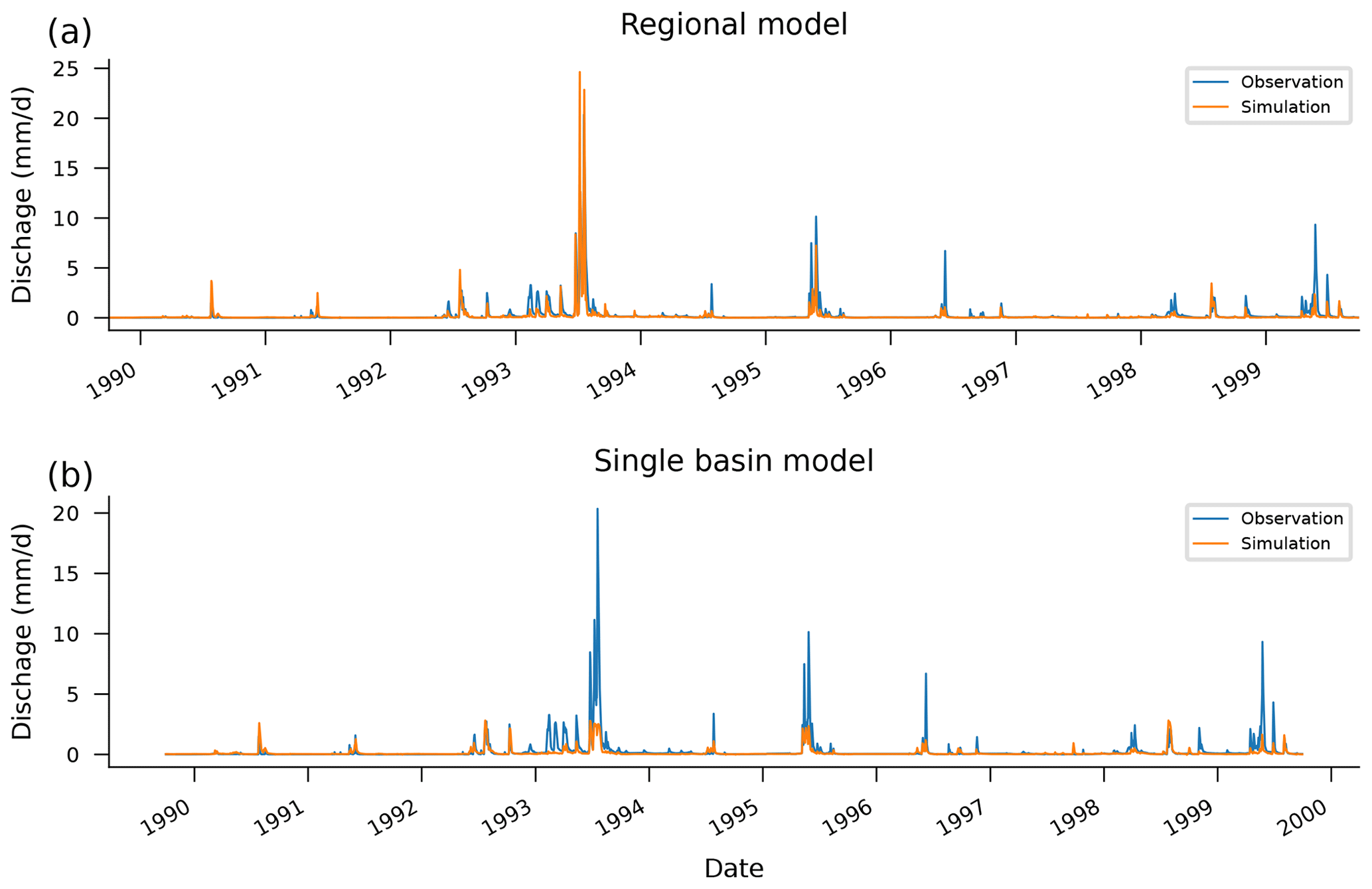
Figure D1 Observed and simulated hydrographs from the test period (1989–1999) in a particular basin (06876700). This gauge is on the Salt Creek in Kansas with a drainage area of 1052 km², and it represents a relatively flashy basin.

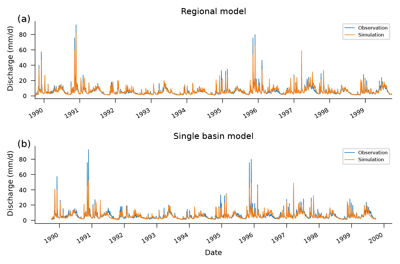
Figure D2 Observed and simulated hydrographs from the test period (1989–1999) in a particular basin (12189500). This gauge is on the Sauk River in Washington, with a drainage area of 1849 km², and represents a basin with high peaks that are not dominated by a seasonal flow pattern.

Appendix E: Other hydrological metrics

There is a large number of metrics that hydrologists use to assess hydrograph simulations (Gupta et al., 2012; Gauch et al., 2023). Several of these metrics are described in Table E1, including bias, correlation, Nash–Sutcliffe efficiency (NSE) (Nash and Sutcliffe, 1970), Kling–Gupta efficiency (KGE) (Gupta et al., 2009), and metrics related to hydrograph peaks. Figure E1 shows differences between regional and single-basin models for these metrics, similarly to the NSE comparison shown in Fig. 3.

The takeaway from this figure is that the main message of this paper (do not train a rainfall–runoff LSTM model on data from a single basin) holds regardless of the metric(s) that we focus on. The skill differences are in correlation-based metrics (NSE, KGE, and Pearson R), as well as variance-based metrics (alpha-NSE). The latter is an artifact of what we saw in Fig. 4, showing that training on a greater number of more diverse data improves the ability of the model to predict high flows. Figure E1 shows only small improvements in the timing and capture of hydrograph peaks (the missed-peaks metric measures whether a peak in the hydrograph was captured at all and not whether the magnitude of the peak was predicted accurately). Furthermore, we see little or no difference in the two bias metrics (beta-NSE, beta-KGE), meaning that improvements to catchment-specific mean discharge are not strongly affected by using training data from multiple catchments (i.e., we do not strongly bias one type of catchment by using other types of catchments in training).

Figure E1 Comparisons between CDFs over 531 CAMELS basins of regional vs. single-basin LSTM models. This is similar to Fig. 3 but for the hydrograph metrics listed in Table E1.

Nash and Sutcliffe (1970)Gupta et al. (2009)Pearson (1895)Gupta et al. (2009)Gupta et al. (2009)Gupta et al. (2009)Gauch et al. (2021)Nearing et al. (2022)

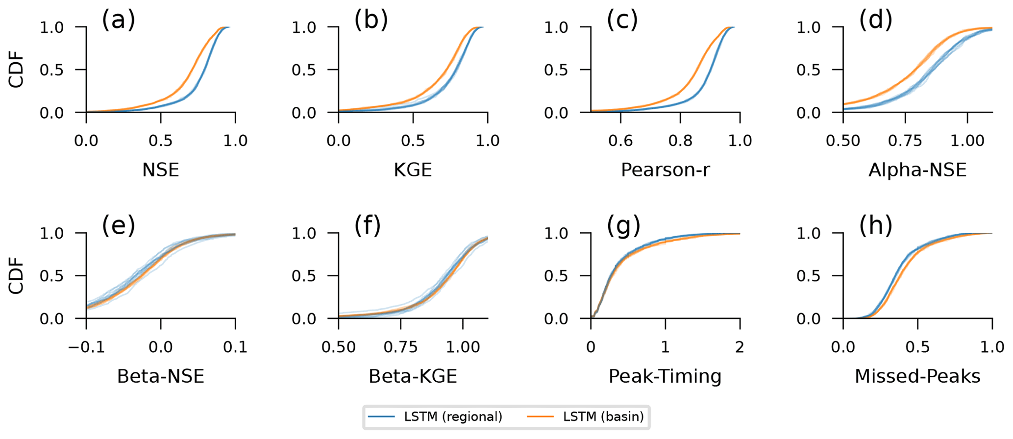
Table E1 A selection of standard hydrograph evaluation metrics.

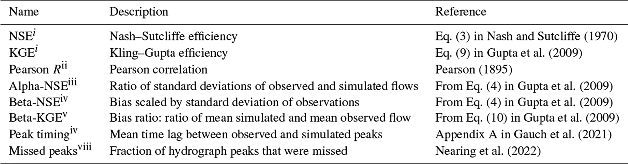
ⁱ (−∞, 1], with values closer to 1 being desirable. ⁱⁱ $[-\mathrm{1},\mathrm{1}]$, with values closer to 1 being desirable. ⁱⁱⁱ (0, ∞), with values close to 1 being desirable. ^iv (−∞, ∞), with values close to zero being desirable. ^v (−∞, ∞), with values close to 1 being desirable. ^vi (0, 1), with values close to zero being desirable.