the Creative Commons Attribution 4.0 License.
the Creative Commons Attribution 4.0 License.
 | 16 Jul 2024
Improving runoff simulation in the Western United States with Noah-MP and VIC models
Lu Su
Dennis P. Lettenmaier
Benjamin Bass
Streamflow predictions are critical for managing water resources and for environmental conservation, especially in the water-short Western United States. Land surface models (LSMs), such as the variable infiltration capacity (VIC) model and the Noah LSM with multiparameterization options (Noah-MP), play an essential role in providing comprehensive runoff predictions across the region. Virtually all LSMs require parameter estimation (calibration) to optimize their predictive capabilities. Here, we focus on the calibration of VIC and Noah-MP models at a ° latitude–longitude resolution across the Western United States. We first performed global optimal calibration of parameters for both models for 263 river basins in the region. We find that the calibration significantly improves the models' performance, with the median daily streamflow Kling–Gupta efficiency (KGE) increasing from 0.37 to 0.70 for VIC, and from 0.22 to 0.54 for Noah-MP. In general, post-calibration model performance is higher for watersheds with relatively high precipitation and runoff ratios, and at lower elevations. At a second stage, we regionalize the river basin calibrations using the donor-basin method, which establishes transfer relationships for hydrologically similar basins, via which we extend our calibration parameters to 4816 hydrologic unit code (HUC)-10 basins across the region. Using the regionalized parameters, we show that the models' capabilities to simulate high and low flow conditions are substantially improved following calibration and regionalization. The refined parameter sets we developed are intended to support regional hydrological studies and hydrological assessments of climate change impacts.
- Article
(5760 KB) - Full-text XML
-
Supplement
(2061 KB) - BibTeX
- EndNote


Streamflow predictions play a key role in water and environmental management, especially in the water-stressed Western United States (WUS). In the short term, these predictions provide early warnings for impending flood events, thereby enabling timely preparation and response to mitigate immediate flood risk and damages (Raff et al., 2013; Maidment, 2017). In the longer term, streamflow predictions enable water utilities and agencies to plan water distribution within and across multiple uses – urban, agricultural, and industrial (Anghileri et al., 2016). Streamflow predictions also aid in understanding and foreseeing the impacts of climate change on water systems, thereby informing adaptive strategies for water resource management.
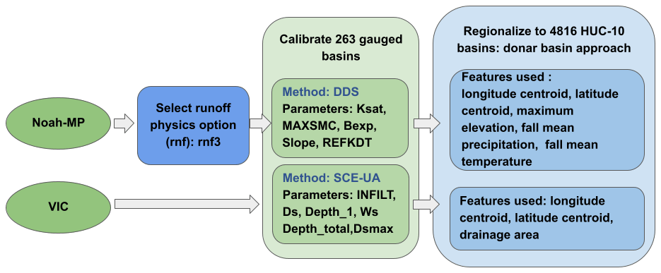
Figure 1(a) Framework of the calibration and regionalization processes adopted in this study. (c) Model simulation inputs and output.
Streamflow predictions are derived via a synthesis of hydrometeorological data, statistical methodologies, and computational modeling. Direct measurement of runoff is an important element of this process; however it is only possible in river basins with well-developed observational infrastructure (Sharma and Machiwal, 2021). This limitation leaves vast areas, often critical to water resource management and climatology, without direct runoff observations on which to base streamflow predictions. As an alternative, land surface models (LSMs) can be used to simulate streamflow. LSMs typically are forced with air temperature, precipitation, and other surface meteorological variables. By integrating climatic, topographic, and land-use information, they can fill streamflow observation gaps and provide comprehensive, spatially distributed runoff predictions (Fisher and Koven, 2020). The capabilities of LSMs equip us with the necessary tools to produce streamflow predictions that can be used to prepare for severe weather conditions, form the basis for water resource management, and inform water management associated with our evolving climate.
One of the key challenges in hydrological modeling is the reliable representation of the spatiotemporal variability of natural processes (Dembélé et al., 2020). Enhanced spatial resolution and improved estimates of surface meteorological variables have empowered LSMs to predict diverse processes with greater detail. However, a recurrent issue is that the parameters embedded in LSMs often inadequately capture fine-scale variations in land surface processes, as illustrated in Figs. S7 and S8 in the Supplement. Accurate prediction of land surface processes, particularly over large areas, requires accurate parameter estimation, which remains a significant bottleneck. Errors in parameter estimates affect LSMs' ability to forecast runoff at continental or subcontinental scales. Fisher and Koven (2020) identify LSM parameter estimation as one of three grand challenges in land surface modeling.
To deal with this challenge, we describe methods and resulting high-resolution parameter datasets for two widely used LSMs across the WUS. We base our estimates on a strategy of minimizing metrics of differences in observed and model-predicted streamflow, following many previous studies (Arsenault and Brissette, 2014; Poissant et al., 2017; Razavi and Coulibaly, 2017; Gochis et al., 2019; Qi et al., 2021; Bass et al., 2023). We do so because streamflow observations are more readily available than other model prognostic variables like soil moisture or evapotranspiration (Demaria et al., 2007; Gao et al., 2019; Troy et al., 2008; Yadav et al., 2007), although the methods we use could be generalized to incorporate other observed and model-predicted fluxes and state variables. Although previous studies have mostly focused on a single hydrologic model (e.g., Mascaro et al., 2023; Sofokleous et al., 2023; Gou et al., 2020), here we utilize two models to address structural model uncertainty and to ensure broader applicability of the calibration methods we employ.
The variable infiltration capacity (VIC; Liang et al., 1994) model and the Noah LSM with multiparameterization options (Noah-MP; Niu et al.. 2011), which we use here, are widely used hydrologic models both in the United States and globally, as highlighted by Mendoza et al. (2015) and Tangdamrongsub (2023). Many previous implementations of VIC for the Western United States (WUS) have been based on the Livneh et al. (2013) dataset, and its predecessor, Maurer et al. (2002), which performed initial calibrations across the region. In the case of Noah-MP, Bass et al. (2023) performed manual calibration across the region. Neither of these implementations, however, employs globally optimized calibration, as we do here.
The process of calibration can be computationally demanding, and prior research typically has focused on obtaining parameters appropriate to facilitating model simulations that match observations as closely as possible at stream gauge locations (Duan et al., 1992; Tolson and Shoemaker, 2007). Most previous studies have concentrated on a limited number of gauges/river basins (e.g., Mascaro et al., 2023; Sofokleous et al., 2023; Gou et al., 2020). Here, we aim to establish parameterizations for VIC and Noah-MP across the entire WUS. In doing so, we apply global optimization methods at 263 river basins, followed by a second stage regionalization to the whole of WUS.
Specifically, the work we report here aims to develop calibration parameters for the VIC and Noah-MP models that can be implemented at the catchment (hydrologic unit code or HUC) 10 level across the region. We explore and elucidate (i) the choice of physical parameterizations and calibration of land surface parameters, (ii) extension of these calibrated parameters to areas without gauges, and (iii) factors that influence calibration efficiency and LSM performance using regional parameter estimates. Following this introduction, Sect. 2 describes our calibration basins, the hydrologic models used, and the forcing dataset. The framework of our procedures is illustrated in Fig. 1. Section 3 provides an in-depth exploration of the calibration process. In the case of Noah-MP, which offers multiple runoff generation (physics) options, our initial step involves choosing the most effective runoff parameterization option. Following this, we perform the calibration of land surface parameters. In the case of the VIC model, the runoff parameterization scheme is predetermined, so we commence immediately with calibration at 263 river basins across our region. Our second stage regionalization (Sect. 4) extends the calibrated parameters to ungauged basins using the technique known as the donor-basin method, as implemented by Bass et al. (2023). In Sect. 5, we evaluate both flood and low flow simulation skills both pre- and post-calibration and following regionalization. Finally, following discussion and interpretation (Sect. 6), Sect. 7 presents conclusions, encapsulating the insights and implications of our study.
2.1 Study basins
We selected 263 river basins distributed across the WUS for calibration of the two models. Most of the basins were from USGS Gages II reference basins (Falcone, 2011) which have minimum upstream anthropogenic effects such as dams and diversions. Among these basins, our selection criteria included having at least 20 years of record and a minimum drainage area of 144 km2, which is the size of four model grid cells. In addition to 250 Gages II reference stations, we included 13 basins located in California's Sierra Nevada for which naturalized flows (effects of upstream reservoir storage and/or diversions removed) are available from the California Department of Water Resources (2021). The locations of the 263 basins are shown in Fig. 2. We used the most recent 20-year period of streamflow observations for calibration in each of the 263 basins.
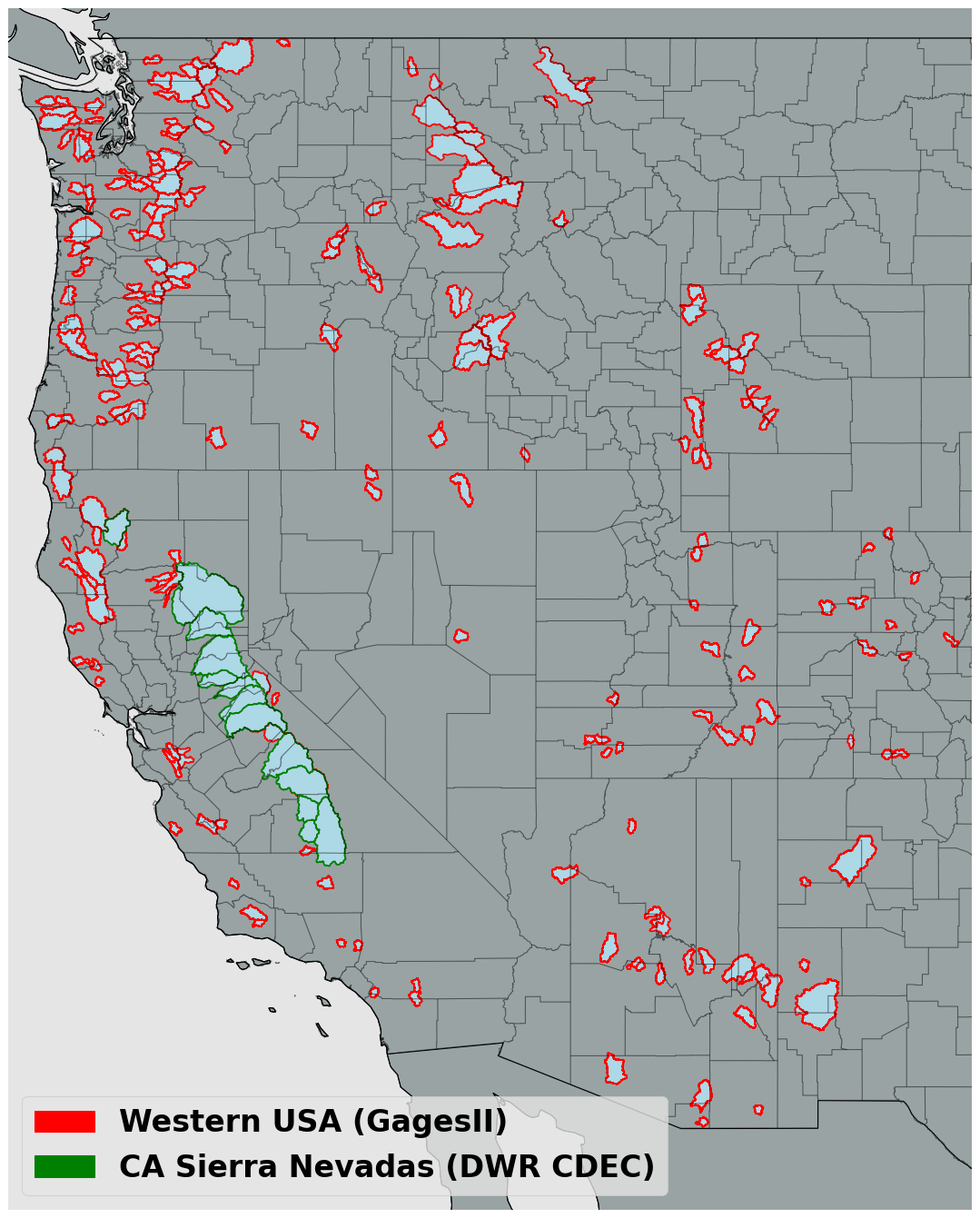
Figure 2A total of 263 river basins for which calibration was performed. The Gages II reference basins are delineated with red boundaries and the CA Sierra Nevada basins with green boundaries.
2.2 Land surface models
The two models we used (VIC and Noah-MP) were chosen due to their broad application and proven effectiveness in hydrological simulations. The VIC model is renowned globally for its success in runoff simulation, as evidenced by studies such as Adam and Lettenmaier (2003), Adam et al. (2006), Livneh et al. (2013), and Schaperow et al. (2021). Conversely, Noah-MP, though relatively newer, forms the hydrologic core of the U.S. National Water Model (NWM) and is increasingly used both within the United States and abroad.
Our selection is further reinforced by a study conducted by Cai et al. (2014), which assessed the hydrologic performance of four LSMs in the United States using the North American Land Data Assimilation System (NLDAS) test bed. This study highlighted Noah-MP's proficiency in soil moisture simulation and its strong performance in total water storage (TWS) simulations, while recognizing VIC's capabilities in streamflow simulations.
Table 1Overview of hydrologic model components and parameter data sources.
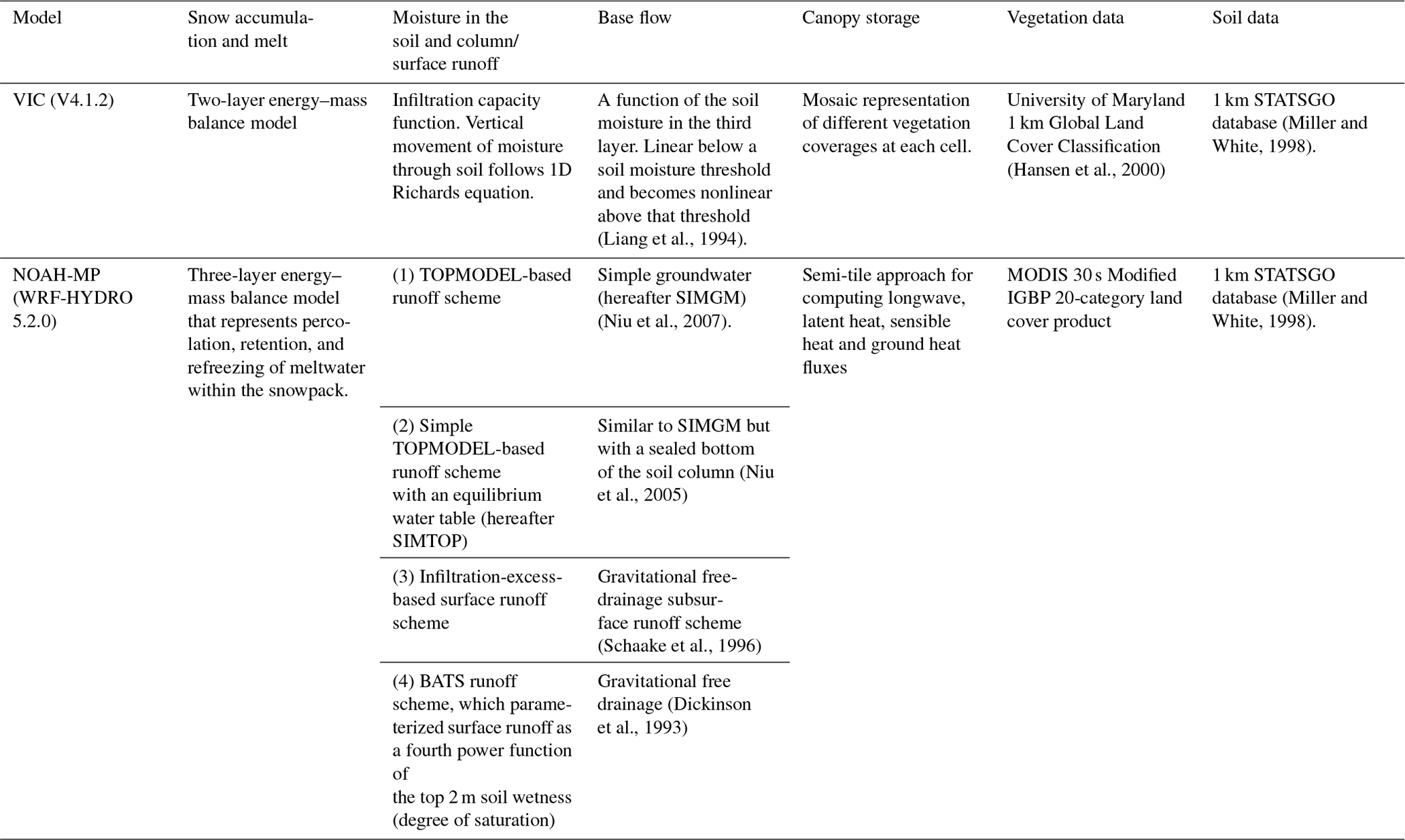
Our choice of models also was informed by the varying levels of complexity these two models offer in conceptualizing the effects of vegetation, soil, and seasonal snowpack on the land surface energy and water balances (refer to Table 1 for more details). VIC and Noah-MP employ different parameterizations for various hydrological processes, such as canopy water storage, base flow, and runoff. Noah-MP features four runoff physics options (see Table 1). It utilizes four soil layers, each with a fixed depth. In contrast, the VIC model, with its variable infiltration capacity approach (Liang et al., 1994), uses up to three soil layers per grid cell with variable depths, providing flexibility in modeling soil moisture dynamics. The unique runoff generation methodologies of each model are particularly pertinent for capturing the diverse hydrological characteristics of the WUS.
The calibrated parameters we develop here for both models will provide future researchers with essential tools for comprehensive hydrological analysis across the WUS. Utilizing these two distinct models, each with unique strengths and methods, will facilitate thorough exploration of the WUS's varied hydrological characteristics and response of the watersheds in the region to climate change, as well as implementation of improved streamflow forecast methods. Our results will help to facilitate a deeper understanding of hydrological processes and spatial variability across the entire WUS region.
In our implementation of both models, we accumulated runoff over each of the calibration watersheds. We chose not to implement the channel routing schemes of either model since their impact on daily streamflow simulations is small given the relatively small size of most of the basins. This aligns with earlier research (e.g., Li et al., 2019). However, in both the case of VIC and Noah-MP, the output of our simulations (runoff) could be used as input to routing models, such as those that are options in the implementation of both models. We describe below the particulars of the two models.
2.2.1 VIC
VIC is a macroscale, semi-distributed hydrologic model (described in detail by Liang et al., 1994) that determines land surface moisture and energy states and fluxes by solving the surface water and energy balances. VIC is a research model, and in its various forms it has been employed to study many major river basins worldwide (e.g., Adam and Lettenmaier, 2003; Adam et al., 2006; Livneh et al., 2013; Schaperow et al., 2021). This model enjoys a broad user community – as per the citation index Web of Science, the initial VIC paper has been referenced more than 2600 times, with contributing authors spanning at least 56 different countries (Schaperow et al., 2021). We obtained initial VIC model parameters from Livneh et al. (2013), who validated model discharges over major continental United States (CONUS) river basins. The origins of the soil and land cover data are outlined in Table 1. The version of the VIC model implemented here is 4.1.2, and it operates in energy balance mode. We selected VIC 4.1.2 for two key reasons: first, our initial parameters were based on Livneh et al. (2013), who validated model discharges over major CONUS river basins using this model version. Second, in a preliminary assessment of snow water equivalent (SWE) simulation skills at select SNOTEL sites across the WUS, we found that VIC 4.1.2 demonstrated superior performance compared to VIC 5 (see Fig. S1). This finding, coupled with our research group's extensive experience and proven results with VIC 4.1.2, informed our decision to use this version.
2.2.2 Noah-MP
Noah-MP was originally designed as the land surface scheme for numerical weather prediction (NWP) models like the Weather Research and Forecasting (WRF) regional atmospheric model. Currently, it is being utilized for physically based, spatially distributed hydrological simulations as a component of the National Water Model (NWM) (NOAA, 2016). It enhances the functionalities of the Noah LSM (as per Chen et al., 1996 and Chen and Dudhia, 2001) previously used in NOAA's suite of numerical weather prediction models by offering multiple options for key processes that control land–atmosphere transfers of moisture and energy. These include surface water infiltration, runoff, evapotranspiration, groundwater movement, and channel routing (see Niu et al., 2007; 2011). The model has been widely used for forecasting seasonal climate, weather, droughts, and floods not only across the continental United States (CONUS) but also globally (Zheng et al., 2019). We utilized the most current version (WRF-HYDRO 5.2.0)
2.3 Forcing dataset
We ran both models at a 3 h time step and at latitude–longitude spatial resolution. The forcings were the gridded observation dataset developed by Livneh et al. (2013) and extended to 2018 by Su et al. (2021) (hereafter referred to as L13). This dataset spans the period from 1915 to 2018. For the VIC model, the L13 dataset provided daily values of precipitation, maximum and minimum temperatures, and wind speed (additional variables used by VIC, including downward solar and longwave radiation and specific humidity, are computed internally using MTCLIM algorithms as described by Bohn et al., 2013). The Noah-MP model, on the other hand, necessitated additional meteorological data such as specific humidity, surface pressure, and downward solar and longwave radiation, in addition to precipitation, wind speed, and air temperature. We used the MTCLIM algorithms, as detailed by Bohn et al. (2013), to calculate specific humidity and downward solar radiation. We employed the Prata (1996) algorithm to compute the downward longwave radiation. Additionally, we deduced surface air pressure by considering the grid cell elevation in conjunction with standard global pressure lapse rates. Following this, we transitioned the daily data to hourly metrics using a cubic spline to interpolate between Tmax and Tmin and derived other variables using the methods explained by Bohn et al. (2013). Lastly, we distributed the daily precipitation evenly across 3-hourly intervals.
We used a 3 h simulation time step given numerical considerations with Noah-MP (which do not affect VIC; however for consistency we used a 3 h time step for VIC as well). Despite the fact that precipitation in particular was available daily (and hence apportioned equally to 3 h time steps), resolving the diurnal cycle is sometimes important in the case of snow (accumulation and ablation) processes which vary diurnally.
3.1 Calibration methods
The initial step in our calibration effort was to optimize the land surface parameters of the two models for the 263 WUS basins. These parameters, primarily soil properties which can exhibit a substantial degree of uncertainty, were iteratively updated via hundreds of simulations to accurately reflect streamflow conditions in each basin.
Our focus on calibrating soil-related parameters was based on their critical role in runoff generation. In this respect, we focused on key processes including infiltration, soil moisture storage, and groundwater recharge. The calibration of parameters that control these processes was prioritized to improve the representation of soil–water interactions, a major driver of runoff variability in the region. Given the importance of snow processes across much of the region, we conducted snow simulation verification at 20 Snow Telemetry (SNOTEL) (Natural Resources Conservation Service, 2023) sites across WUS. Our assessment (see Fig. S1) indicated that the existing parameterizations for snow processes in both models reproduced observed SWE well across our study region.
Table 2Calibration methods, parameters, and modifications to their initial default values evaluated in the calibration.
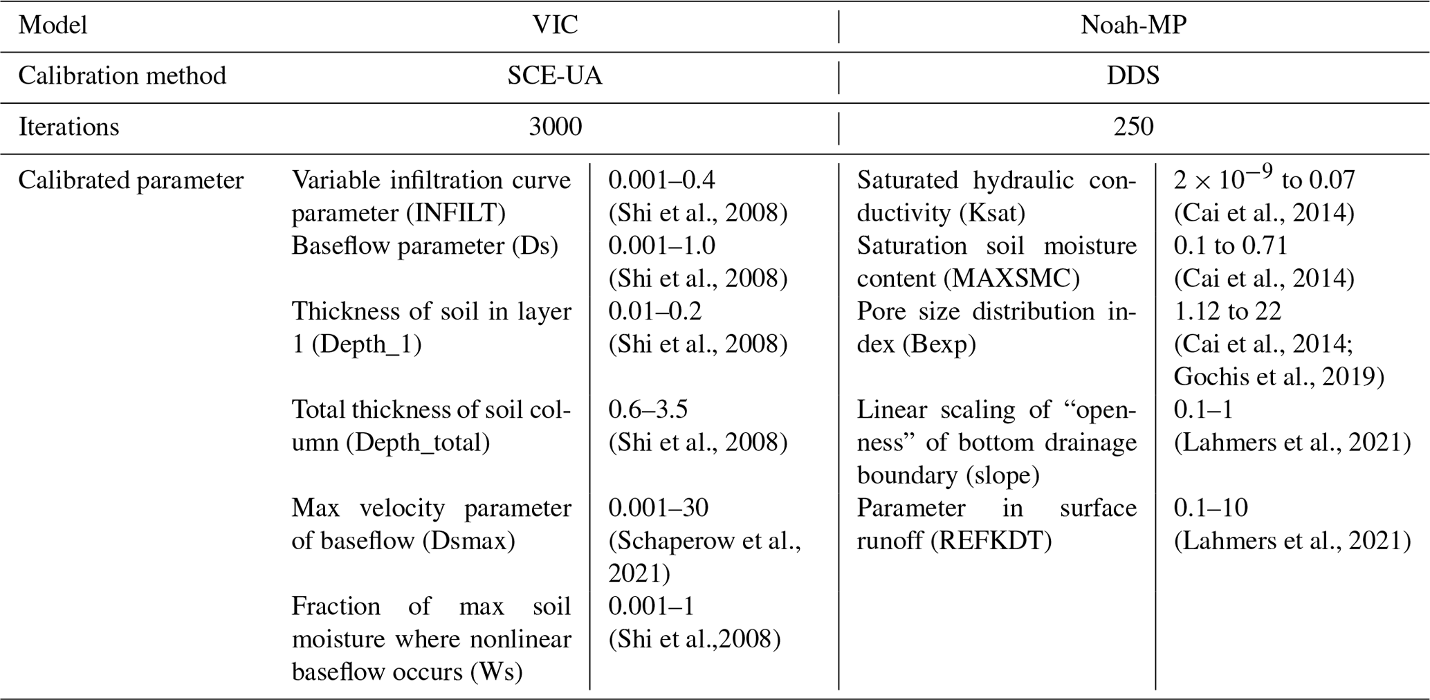
Prior to calibration, we conducted a sensitivity analysis to identify the most influential parameters for streamflow simulation in both models. We also drew on insights from previous research in this respect (Mendoza et al., 2015; Hussein, 2020; Shi et al., 2008; Holtzman et al., 2020; Bass et al., 2023; Schaperow et al., 2021). We then performed a sensitivity analysis, focusing on how variations in the most sensitive parameters impacted Kling–Gupta efficiency (KGE; Gupta et al., 2009). Based on these analyses, we chose to calibrate six parameters for the VIC model and five for the Noah-MP model (Table 2). For each parameter, we defined a physically viable range (refer to Table 2), drawing from values utilized in prior studies (Cai et al., 2014; Mendoza et al., 2015; Hussein, 2020; Shi et al., 2008; Gochis et al., 2019; Holtzman et al., 2020; Lahmers et al., 2021; Bass et al., 2023; Schaperow et al., 2021).
In recent years, the development of hydrologic model calibration has evolved from manual, trial-and-error approaches to advanced automated techniques. This has included a shift towards global optimization methods, notably the Shuffled Complex Evolution algorithm (SCE-UA; Duan et al.,1992). Typically, SCE-UA has been applied to computationally efficient models (simulation time often on the order of a few minutes or less; see, e.g., Franchini et al., 1998). However, its application becomes less practical with more recent distributed hydrologic models such as the Noah-MP, which require longer simulation times. To address these computational challenges, Tolson and Shoemaker (2007) introduced the Dynamically Dimensioned Search (DDS) algorithm, tailored for complex, high-dimensional problems. DDS is more computationally efficiency than SCE-UA, and we therefore used it for our Noah-MP calibrations.
To assure that the parameter sets we estimated were not dependent on the optimization method, we conducted a comparison between SCE-UA and DDS for calibrating VIC across 20 randomly chosen basins. We found that the DDS algorithm achieved optimal calibration with fewer iterations (typically around 3000 iterations vs only about 250 for DDS). The parameter sets identified were nearly identical, affirming our decision to use distinct algorithms tailored to the computational demands of each model.
For both models, our objective function was the KGE metric for daily streamflow. KGE is a widely used performance measure because of its advantages in orthogonally considering bias, correlation, and variability (Knoben et al., 2019). KGE = 1 indicates perfect agreement between simulations and observations; KGE values greater than −0.41 indicate that a model improves upon the mean flow benchmark (Konben et al., 2019).
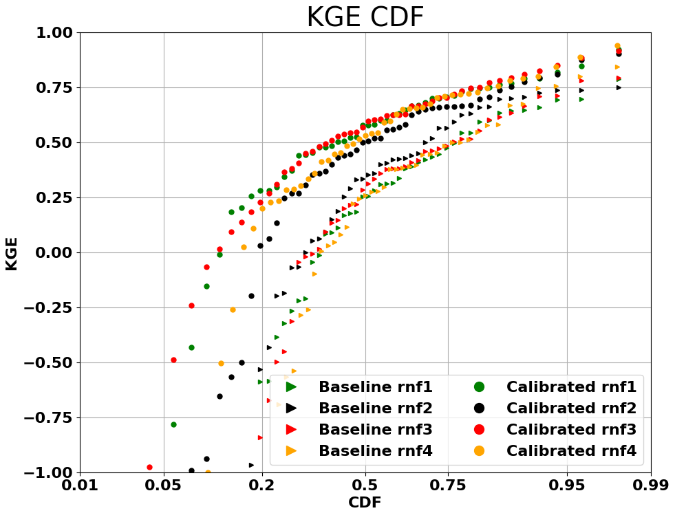
Figure 3Streamflow performance (KGE of daily streamflow simulations) of different Noah-MP runoff generation options across 50 (of 263) randomly selected basins. The performances are shown for both baseline and calibrated simulations.
3.2 Noah-MP parameterization
As specified in Table 1, Noah-MP has four runoff and groundwater physics options (rnf). Initially, we adopted the options that are incorporated in the NWM, as elaborated in Gochis et al. (2020). Before we could proceed with calibrating Noah-MP for all the WUS basins, it was necessary to determine suitable rnf's. To streamline computational time, we initially selected 50 basins randomly from the total of 263 from which we created four experimental groups. Each group employed a different rnf option. We applied the DDS method to these groups and compared the cumulative distribution functions (CDFs) of their baseline and calibrated KGEs (Fig. 3). From this figure, it is apparent that the KGE improved post-calibration for all four rnf's. Notably, rnf3, also known as free drainage, exhibited the most substantial performance enhancement after calibration. As a result, we chose to continue using this option, which is incorporated in the NWM. Nonetheless, it is worth noting that the use of different options for different basins – a feature currently not utilized in Noah-MP or WRF-Hydro – could potentially result in improved overall model performance.
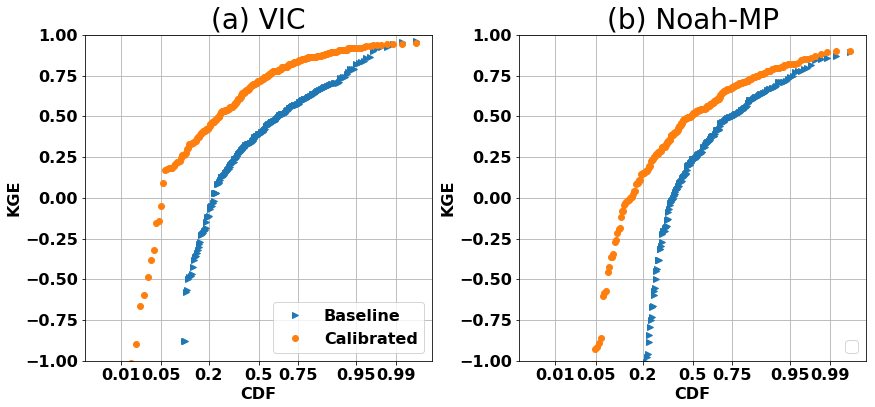
Figure 4Cumulative distribution function (CDF) plot of the daily streamflow KGE for (a) VIC and (b) Noah-MP, comparing baseline and calibrated runs across all 263 basins.
3.3 Calibration of gauged basins
Following the selection of the most effective set of runoff generation options across the domain, we estimated model parameters for all 263 basins. The comparative performance of the models, before and after calibration, is shown in Fig. 4. It is apparent from the figure that both Noah-MP and VIC have significantly enhanced their daily streamflow simulation skills post-calibration. After calibration, the median KGE of Noah-MP improved from 0.22 to 0.54, and the VIC's median KGE increased from 0.37 to 0.70. When contrasting the two models, we observed that VIC outperformed Noah-MP both pre- and post-calibration. One possible explanation could be that the baseline VIC parameters were taken from Livneh et al. (2013), and these parameters had already been validated and adjusted for major US basins (although not for our 263 basins specifically), while the Noah-MP parameters are default values from NWM. Another possibility is inherent differences in the physics of streamflow simulation between the two models (VIC primarily generates runoff via the saturation excess mechanism), although that is not the main focus of our research.
Following the calibration with data from the past 20 years, we performed a test where we calibrated the streamflow using the first 10 years of data and validated with the subsequent 10 years of data. This test revealed that the KGE distribution from the 10 year calibration is similar to that from the 20 year data. The median KGE values for VIC and Noah-MP after calibration with 10 years of observations were 0.52 and 0.69, respectively. Correspondingly, the median KGEs during the validation period were 0.50 and 0.68, respectively, which are only slightly lower. These comparisons demonstrate general consistency over time in the performance of the calibrated parameters.
To validate the robustness of our calibration methodology, we calculated alternative (to KGE) performance metrics, specifically the Nash–Sutcliffe efficiency (NSE) and bias. Our analyses, detailed in Figs. S2 and S3, revealed significant enhancements in model performance as measured by these metrics. The observed improvements across multiple evaluation criteria affirm the efficacy of our calibration process and in particular that the performance of our procedures is not contingent upon the choice of evaluation metrics.
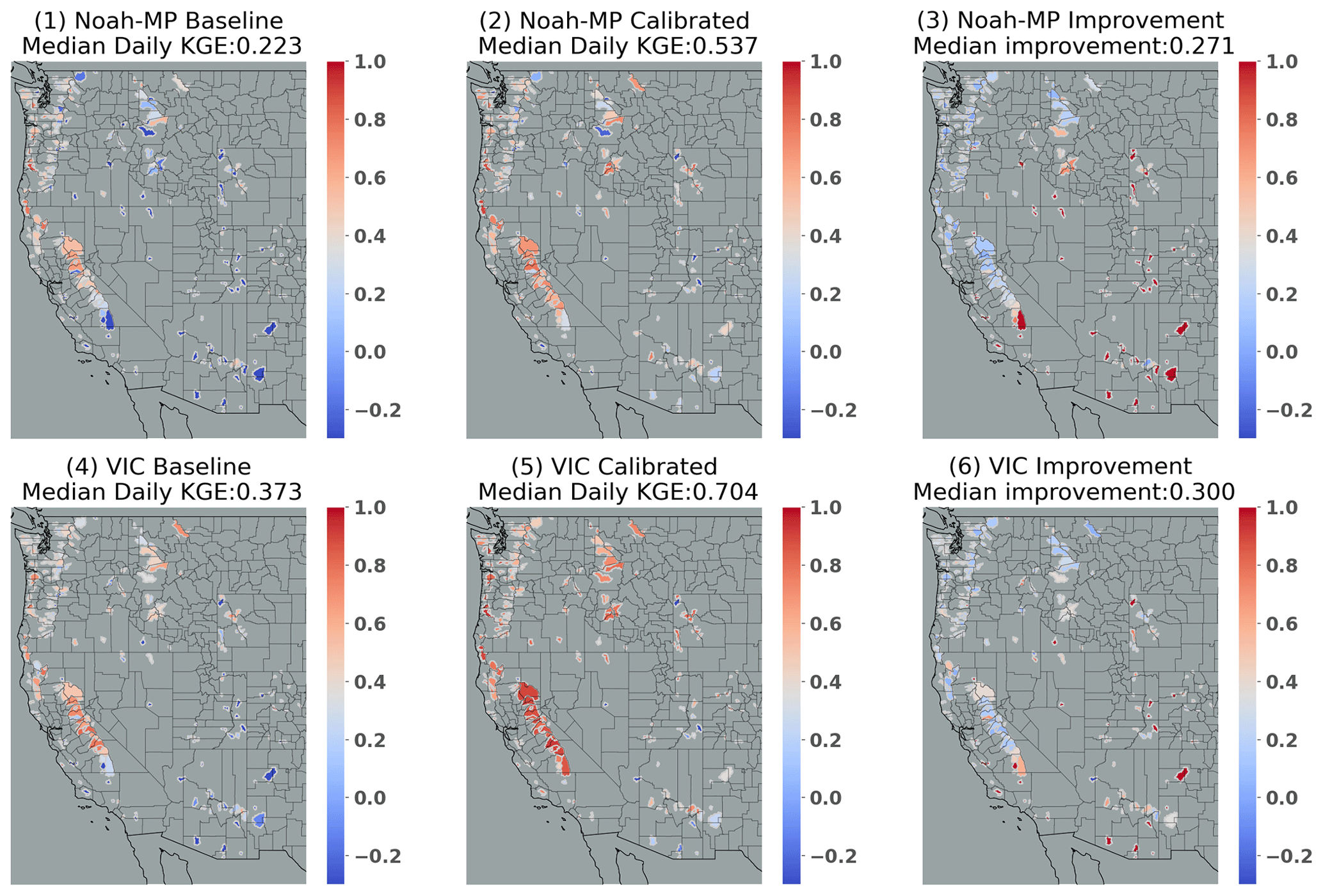
Figure 5Spatial distribution of daily streamflow KGE for Noah-MP baseline (1), calibrated Noah-MP (2), difference between calibrated and baseline Noah-MP (3), VIC baseline (4), calibrated VIC (5), and difference between calibrated and baseline VIC (6).
We examined the spatial variability of daily streamflow KGE for Noah-MP and VIC, both before and after the calibration (see Fig. 5). The highest baseline KGEs are along the Pacific coast, in central to northern CA, for both models. VIC's baseline KGE generally is high in the Pacific Northwest. Post-calibration improvements occurred for both models in most areas, especially in regions where the baseline KGE was low, such as southern CA and the southeastern part of the study region. Median improvements after calibration were 0.27 for Noah-MP and 0.30 for VIC.
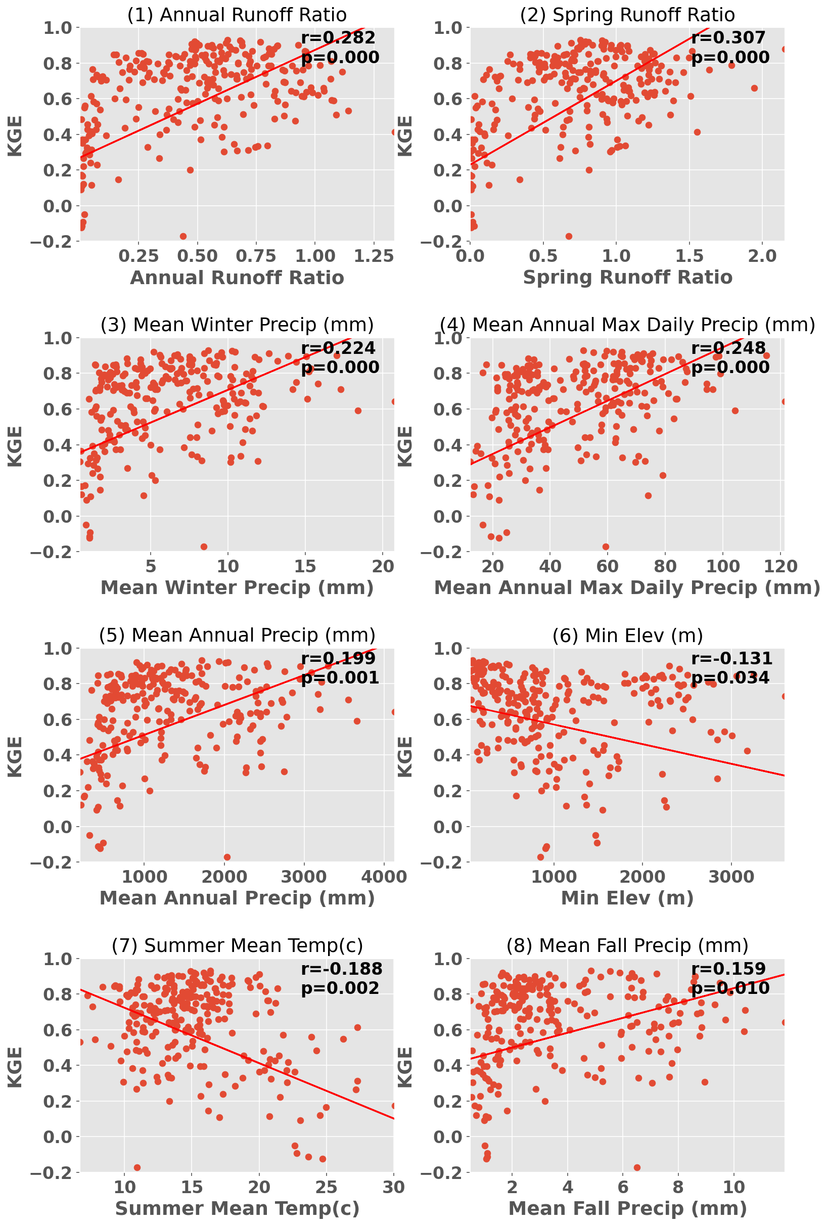
Figure 6Scatter plots of VIC KGE in relation to significantly correlated characteristics. Each subplot indicates the corresponding Pearson correlation coefficients and the P value.
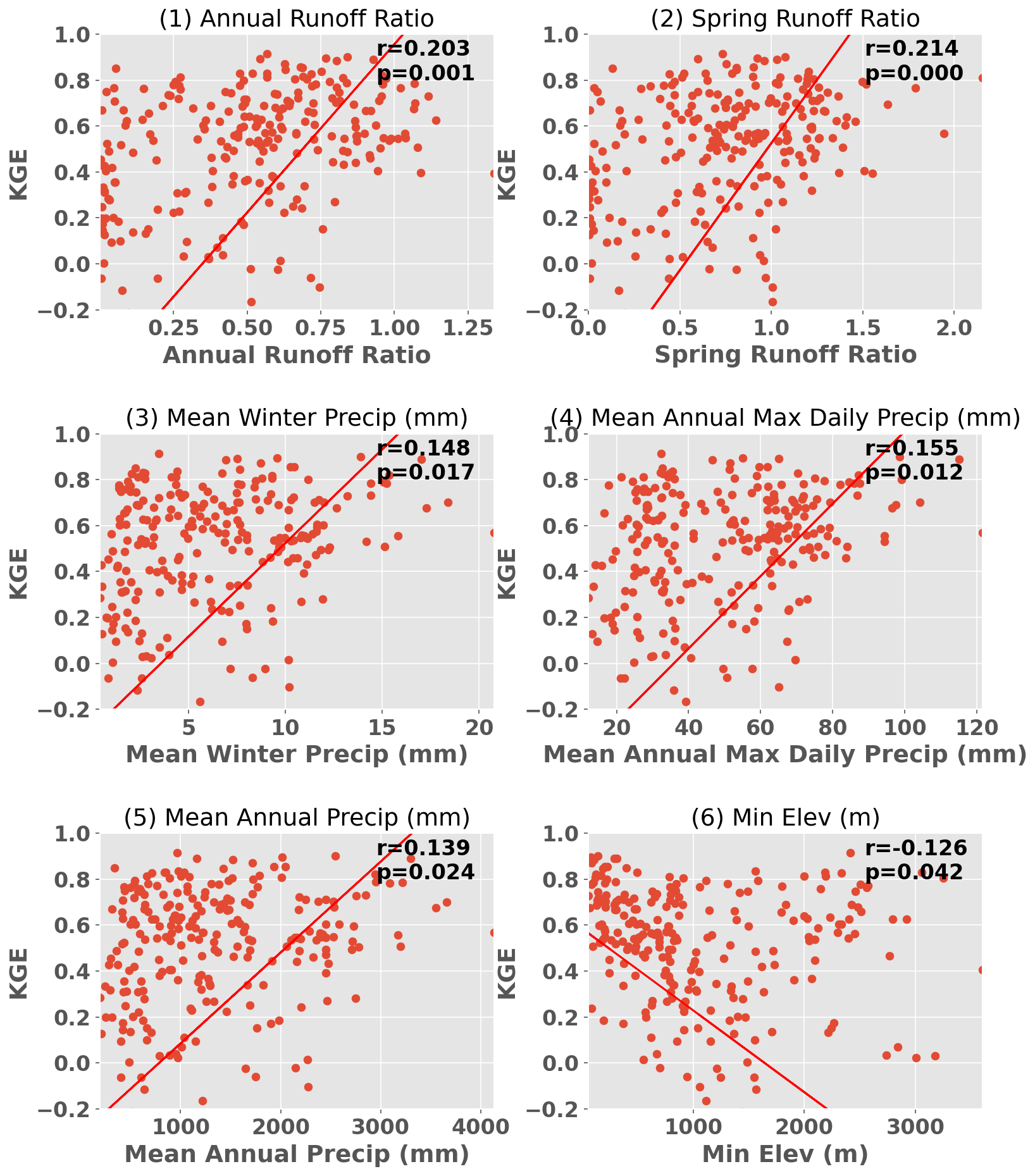
Figure 7Scatterplot of Noah-MP KGE in relation to significantly correlated characteristics. Each subplot indicates the corresponding Pearson correlation coefficients and the P value.
We observed that basins displaying higher KGE values typically were more humid than those with lower KGE. To further delve into the relationship between KGE and basin characteristics, we explored correlations between KGE and 21 different characteristics, including drainage area, elevation, seasonal/annual average temperature and precipitation, annual maximum precipitation, and seasonal/annual runoff ratio. Of these, 12 characteristics were statistically significantly correlated with the VIC KGE, including four seasonal and annual runoff ratios; mean precipitation in winter, spring, and fall; annual maximum precipitation; and minimum elevation. Figure 6 shows scatter plots of eight representative characteristics. Apart from minimum elevation and mean summer temperature, all other characteristics were positively correlated with KGE. Typically, spring runoff ratio, annual runoff ratio, mean annual max precipitation, and mean winter precipitation exhibited the highest correlations with KGE. This implies that basins with higher runoff ratios (particularly in spring), higher precipitation (especially maximum precipitation), lower summer temperature, and lower elevation are more likely to exhibit strong VIC performance. The same applies to Noah-MP, as indicated in Fig. 7, although Noah-MP showed relatively weaker correlations. Correlations between mean summer temperature and mean fall precipitation and Noah-MP KGE were not statistically significant.
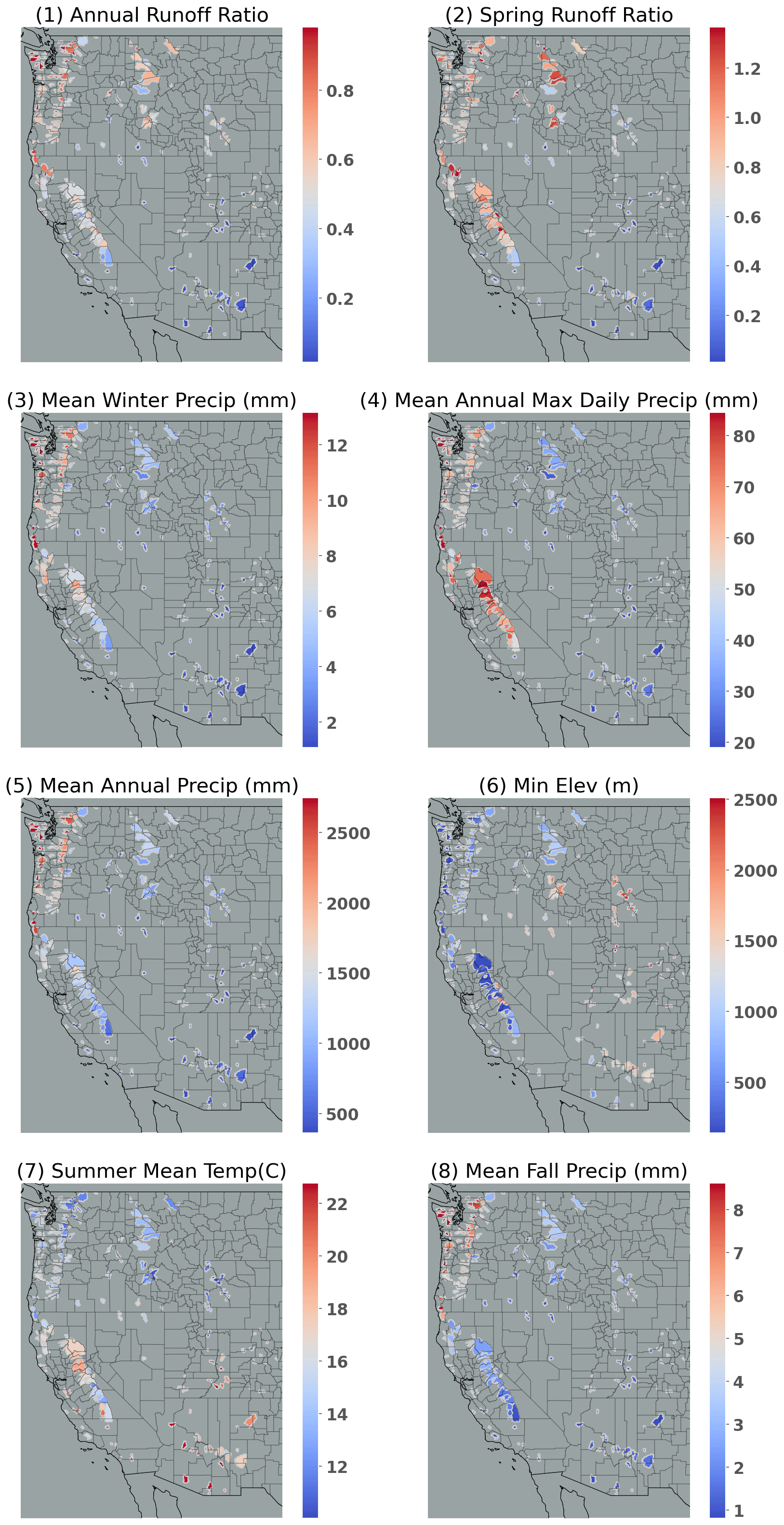
Figure 8Spatial distribution of characteristics that are statistically significantly correlated with KGE. Note that all characteristics are significantly correlated with VIC KGE, whereas only (1)–(6) are significantly correlated with Noah-MP KGE.
The spatial distribution of the eight characteristics is qualitatively similar with the KGE spatial distribution, as shown in Fig. 8. Generally, basins with higher KGE have higher characteristic values when the correlation is positive and lower characteristic values when the correlation is negative. As noted above, both models show good baseline performance along the Pacific coast and in central to northern CA (Fig. 5). Those areas have high runoff ratios (specifically spring and annual) and high mean winter precipitation. These features generally lead to runoff physics that are dominated by the saturation-excess mechanism, which is well represented by both VIC and Noah-MP. VIC's baseline KGE generally is high in the inland Northwest which has somewhat lower runoff ratios and (relatively) deeper groundwater tables. VIC's superior performance relative to Noah-MP may also be because of its variable rather than fixed soil moisture depths (as is the case for Noah-MP).
To distribute parameters from the calibration basins to the entire region, we used the donor-basin method as implemented in numerous previous studies (e.g., Arsenault and Brissette, 2014; Poissant et al., 2017; Razavi and Coulibaly, 2017; Gochis et al., 2019; Qi et al., 2021; Bass et al., 2023). Following the calibration process, we regionalized the parameters from gauged to ungauged basins based on a mathematical assessment of the spatial and physical proximity between the gauged and ungauged basins. We considered two primary methods for implementing the donor-basin approach. The first uses models calibrated to spatially continuous gridded runoff metrics (Beck et al., 2015; Yang et al., 2019). The second approach, which we ultimately adopted, calibrates models to individual gauges and then extends these parameters to ungauged basins, based either on a statistical or mathematical similarity measures (e.g., Arsenault and Brissette, 2014; Razavi and Coulibaly, 2017). Our preference for the second method was guided by a key limitation of the first approach; specifically it is limited to calibrating against runoff metrics, such as long-term mean flow and flow percentiles, rather than streamflow time series.
In the donor-basin method, an ungauged basin inherits its land surface parameters from the most similar gauged basin(s) (or the n most similar gauged basins). Here, we evaluated the similarity or proximity between gauged and ungauged basins based on the similarity index SI as defined and used by Burn and Boorman (1993) and Poissant et al. (2017):
In Eq. 1, k stands for the total number of features considered; represents the ith feature of the gauged basin G; is the ith feature of a specific ungauged basin; and ΔXi is the range of potential values for the ith feature, grounded in the data from the gauged basins. This yields a unique value of SI for each gauged basin, contingent on the specific ungauged basin it is compared with. Typically, gauged basins that exhibit greater resemblance to the ungauged basin will have a smaller SI.
We assessed the donor-basin method's efficacy using a cross-validation approach, where each gauged basin was treated as ungauged one at a time. The pseudo-ungauged basin inherits its hydrological parameters from its three most similar gauged basins, determined by SI. The parameters inherited are a weighted average from the three donor basins. After testing one to five donor basins, we found that using three donors yielded the best results. Thus, every basin inherits parameters from the three most similar gauged basins in each simulation, offering a concise evaluation of the donor-basin method's regionalization performance.
We used 18 basin-specific features in the donor-basin method, detailed in Table S1 in the Supplement, calculated based on the forcings and parameters used in the study. For feature selection in the donor-basin method, we adopted an iterative approach, explained in detail in the following paragraph. Only basins with a KGE exceeding 0.3 were considered, following previous studies suggesting that inclusion of poorly performing basins can lower regionalization performance. We found that a KGE threshold of 0.3 resulted in a median performance improvement of 0.08 larger than a KGE threshold of 0 did; hence it was chosen. After screening, 223 basins were utilized in VIC regionalization and 194 in Noah-MP regionalization. We note that the parameters used for calibration and the features used to determine the similarity index in the regionalization process are different. The physics that control the key hydrological processes of the two models are different, so we explored their best regionalization features separately.
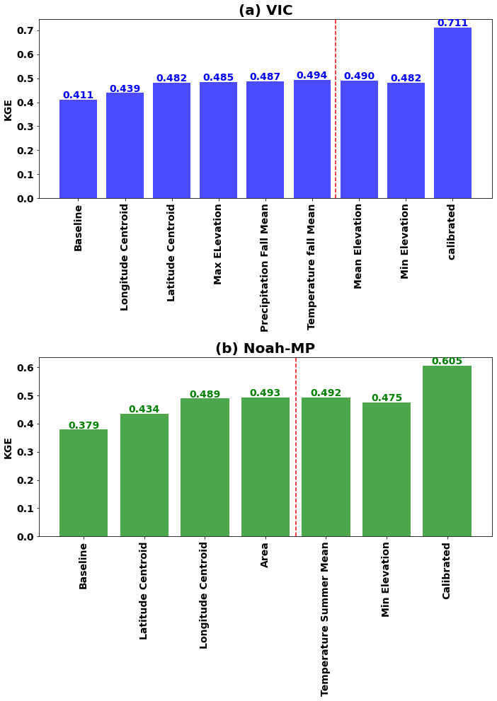
Figure 9Best regionalization features for (a) VIC and (b) Noah-MP. The final regionalization to ungauged basins of the WUS incorporated all features up to the point marked by the red line since the addition of further features does not improve KGE.
To determine the most effective regionalization features from the 18 basin characteristics listed in Table S1, we employed a systematic iterative approach. The first iteration includes 18 simulations, each of which incorporates one of the 18 features. The feature that yielded the greatest increase in the median KGE across all basins, based on leave-one-out cross validation, was then retained. In the second iteration, we conducted 17 simulations, each combining the retained feature from the first iteration with one of the remaining 17 features. This process was repeated iteratively, reducing the number of features considered in each subsequent round, until the addition of new features no longer resulted in an appreciable increase in median KGE. The sequence of features shown in Fig. 9 (also shown in Table S1) indicated the importance of the features. This iterative approach ensured that each feature's individual and combined contribution to model performance was thoroughly assessed. It allowed us to identify a subset of features that, when used together, optimally improved model accuracy. We recognize the potential existence of inter-feature correlations that may exert a discernible influence on their collective efficacy when utilized in combination.
This procedure resulted in five features that generated the best regionalization performance for VIC (longitude centroid, latitude centroid, maximum elevation, fall mean precipitation, and fall mean temperature). Three features were found to be best for Noah-MP (latitude centroid, longitude centroid, and drainage area) (see Fig. 9). Among them, latitude and longitude are the common features that contribute the most to regionalization when using the similarity index method. This suggests that geographical similarities are the most important factor in parameter information transfer from gauged to ungauged basins.
Upon evaluating the performance of baseline, calibrated, and regionalized simulations, the respective median daily KGEs for the VIC model were found to be 0.41, 0.71, and 0.49. For the Noah-MP, these values were 0.38, 0.60, and 0.49 (refer to Figs. 9 and S4). These metrics are for basins that have a calibrated KGE greater than 0.3 only, resulting in higher median KGEs than for all 263 basins (see Fig. 4). The KGE distribution also improved overall. It is noteworthy that the regionalization improvement relative to baseline is higher for Noah-MP than for VIC. While VIC's baseline and calibrated KGE skill distributions outperform Noah-MP's, the differences between regionalized skills of Noah-MP and VIC are decreasing. We will explore more on this in the following section.
After optimizing the features and specific design of the donor-basin method, parameters were regionalized to 4816 ungauged USGS hydrologic unit code (HUC)-10 basins across the WUS. HUCs are delineated and quality-controlled by USGS using high-resolution DEMs. For each of the 4816 HUC-10 basins, we calculated a similarity index with the calibrated basins using the selected features. The three most similar basins were identified as donor basins, and their weighted average parameters were then adopted by the target HUC-10 basin. The final hydrologic parameters for both VIC and Noah-MP for all WUS HUC-10 basins are shown in Figs. S5 and S6. The baseline HUC-10 parameters are shown in Figs. S7 and S8.
Comparison of Figs. S5 and S6 to S7 and S8 makes it clear that the baseline model parameters lack accuracy and exhibit significant spatial uniformity where large geographical regions share identical parameter values. For example, parameters such as Ds and Soil_Depth1 in VIC show this uniformity. Furthermore, certain parameters, such as SLOPE and REFKDT in Noah-MP, remain invariant across all spatial domains and do not reflect real-world conditions. Regionalization improved the parameters, leading to increased accuracy and strengthening of region-specific characteristics.
Our primary calibration objective was to enhance the accuracy of daily streamflow simulations. However, to ensure the versatility of our parameter sets for research related to both floods and dry conditions, we also evaluated the models' capabilities in reproducing high and low streamflow. To understand the capabilities of the two models in reconstructing high and low streamflow, we assessed their performance across baseline, calibrated, and regionalized settings.
- a.
Evaluation of high flow performance.
We used the peaks-over-threshold (POT) method (Lang et al., 1999) to identify extreme streamflow events as in Su et al. (2023a) and Cao et al. (2019, 2020). We first applied the event independence criteria from USWRC (1982) to daily streamflow data to identify independent events. We set thresholds at each basin that resulted in three extreme events per year on average (denoted as POT3). After selecting the flood events over the study period based on the observation, we sorted the floods based on the return period and then calculated the KGE of baseline, calibrated, and regionalized floods. Figure S9 displays the associated CDF plots. The median KGE for baseline floods in Noah-MP was 0.14, which rose to 0.37 post-calibration and receded to 0.22 after regionalization. For VIC, the flood KGE started at 0.11, increased to 0.41 after calibration, and declined to 0.20 post-regionalization. As anticipated, these numbers are lower than (all) daily streamflow skill due to our calibration target being daily streamflow. Still, flood competencies experienced considerable enhancement, surpassing the Noah-MP KGE benchmark of −0.41 found by Knoben et al. (2019).
- b.
Evaluation of low flow performance.
To assess low flow performance, we utilized the 7q10 metric. This hydrological statistic, commonly adopted in water resources management and environmental engineering, is the lowest 7 d average flow that occurs (on average) once every 10 years (EPA,2018). Scatter plots of 7q10 (Fig. S10) showed high correlation between our model's simulated low flows and the observed data. Post-calibration, this alignment intensified. The VIC model tended to underestimate the low flows. After calibration, the median bias improved from −23.6 % to −9.9 %, and with regionalization, it was −11.7 %. In contrast, Noah-MP began with an 11.20 % overestimation in the baseline, which improved to 0.61 % post-calibration and was −9.5 % after regionalization. The outcomes underline the proficiency of both models for low flow prediction, exhibiting enhanced competencies post-calibration and commendable performance after regionalization.
- c.
Comparison of VIC and Noah-MP simulation skill.
In Sect. 4, we demonstrated that while VIC's baseline and calibrated daily streamflow KGE skill distributions were better than Noah-MP's, the disparity was reduced following regionalization. We further explored the skill differences between the two models for baseline, calibrated, and regionalized parameters for different hydroclimatic conditions. Figure 10 shows the CDF of the daily streamflow KGE differences between VIC and Noah-MP across the study basins. The skill gap between VIC and Noah-MP generally narrows from the baseline through calibrated to regionalized runs, although VIC outperforms Noah-MP in most of the basins for all three runs.
We further divided the study region into four different categories following Huang et al. (2022): coastal-snow-dominated basins, coastal-rain-dominated basins, interior wet basins, and interior dry basins. In the baseline runs (Figs. 10 and 11 (1)), VIC generally outperforms Noah-MP with a median KGE difference of 0.168, particularly in interior dry basins, and in some interior wet and coastal basins. Following calibration (Figs. 10 and 11 (2)), the median KGE difference decreases to 0.126. VIC has superior performance in most of the basins, especially interior wet and coastal basins. In interior dry basins (mostly in the southeastern part of our domain), VIC's performance is similar to or worse than Noah-MP's. This discrepancy is attributable to more pronounced improvements in VIC after calibration in coastal and northern WUS, while Noah-MP shows greater improvements in the southeastern WUS (mostly dry interior). Post-regionalization (Figs. 10 and 11 (3)), the KGE differences further narrow to a median of 0.054, with VIC still outperforming Noah-MP in most coastal and interior wet basins. Nonetheless, VIC is inferior in a few interior dry basins scattered across WUS, where both models exhibit relatively low skill. This is also shown in Fig. S11 CDFs, which indicate that VIC's performance varies notably across the spectrum: it falls below Noah-MP at the lower end of the skill distribution. Conversely, VIC KGEs exceed those of Noah-MP in areas where its skill is strongest. Across all basins collectively, VIC outperforms Noah-MP post-regionalization, as evidenced by higher VIC median skill (Fig. 10 inset).
We also evaluated the performance of the two models after regionalization in simulating annual average flows, flood flows (POT3), and low flows (measured as 7q10). The results (see Figs. S12 and S13) show that VIC outperforms Noah-MP in simulating annual mean streamflow (Fig. S12) and (in most cases) floods (Fig. S13). Conversely, Noah-MP generally performs better in simulating low flows (Fig. S10).
- d.
Comparison of post-regionalization and post-calibration performance.
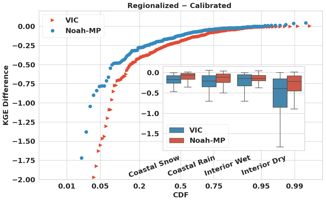
We further analyzed the performance differences between the regionalized and calibrated runs for each model. As depicted in Fig. 12, both VIC and Noah-MP have declining skill for post-regionalization relative to post-calibration runs, with VIC demonstrating a more pronounced decrease, reflected in a median KGE difference of −0.199, compared to −0.117 for Noah-MP. For both models, coastal basins and interior wet basins tend to have smaller skill decreases from post-calibration to post-regionalization, and interior dry basins have the largest skill decreases. VIC has greater decreases than Noah-MP in most basins. The most significant drops in performance generally occur in basins where baseline skills are low, yet post-calibration skills are relatively high.
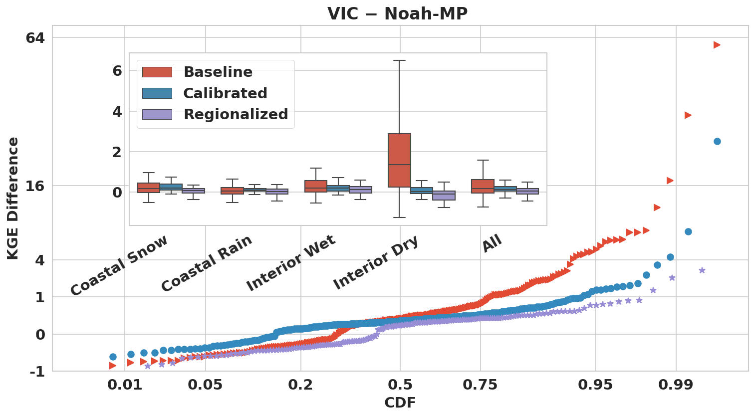
Figure 10Cumulative distribution function (CDF) plot of the daily streamflow KGE differences between VIC and Noah-MP in the study basins for baseline, calibrated, and regionalized runs. The inset figure shows box plots of KGE differences for four different categories: coastal-snow-dominated basins (54 basins), coastal-rain-dominated basins (103 basins), interior wet basins (53 basins), and interior dry basins (53 basins). We also show all basins collectively (263 total) for reference purposes.
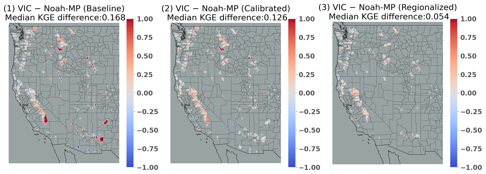
Figure 11Map of the daily streamflow KGE differences between VIC and Noah-MP in the study basins for (1) baseline, (2) calibrated and (3) regionalized runs.
We summarize our key accomplishments in calibrating the two hydrological models, we examine our approach to choosing calibration objective functions and metrics, and we consider lessons learned in model regionalization.
- a.
Improved parameter sets.
We generated calibrated parameter sets for the VIC and Noah-MP hydrological models at ° latitude–longitude scale across WUS. These calibrated parameter sets are intended to facilitate the use of the two models for climate change and water investigations across the region, among other applications. Our focus on calibrating daily streamflow aligns with common practice in hydrology, providing a comprehensive representation of catchment hydrology dynamics which should enhance future understanding of hydrological phenomena and their spatial variations across the region.
- b.
Selection of calibration objective function.
We used objective functions based on streamflow observations. We chose this approach due to its applicability elsewhere, given the widespread accessibility of streamflow observations as compared to alternative metrics such as soil moisture or evapotranspiration (Demaria et al., 2007; Gao et al., 2019; Troy et al., 2008; Yadav et al., 2007). While we acknowledge the potential of remote sensing products like MODIS, SMAP, SMOS, ESA, and ALEXI to improve calibration efforts, especially for variables like actual evapotranspiration (AET) and soil moisture (SM), we were limited by the scarcity of observations for these variables. Future studies could, nonetheless, leverage from the methods we have employed to incorporate additional variables into the objective functions we used.
- c.
Selection of calibration metric.
We used the KGE metric applied to daily streamflow, which we chose for its ability to address bias, correlation, and variability simultaneously (Knoben et al., 2019). We also evaluated NSE and bias metrics, and found substantial improvements in both models' performance after calibration when these metrics were used in place of KGE (See Figs. S2 and S3). Our assessment of high and low flow reconstruction in Sect. 5 further validated our generated parameter sets. While we used a single objective function due to data and computing constraints, incorporating multiple objective functions is feasible in principle.
- d.
Regionalization possibilities.
We calibrated model parameters directly for individual basins, considering their unique hydrological features, and then transferred these calibrated parameters to similar basins based on similarity assessments. Alternative parameter transfer strategies could be used within the same framework we employed (e.g., pedo-transfer functions, e.g., Imhoff et al.,2020) or multiscale parameter regionalization (e.g., Schweppe et al.,2022). We do note that our regionalization approach facilitates the transfer of calibrated parameters to comparable regions, which could be explored in future research.
Our intent was to develop a regional parameter estimation strategy for the VIC and Noah-MP land surface schemes and to apply it across the WUS region at the HUC-10 catchment scale. We have described what we believe is a robust framework that can be applied in future hydrological and climate change studies across the WUS and is applicable to other regions as well. Our key findings and conclusions are given in the following.
Our catchment-scale calibration of the two models to 263 sites across WUS resulted in major improvements in the performance of both models relative to a priori parameters, but performance improvement was the greatest for Noah-MP – although this may be in part because VIC a priori parameters benefitted from prior calibration and hence resulted in better baseline performance than the a priori Noah-MP did.
Both models performed best in more humid basins, mainly in the Pacific Northwest and central to northern CA where runoff ratios are high. This is consistent with previous results (e.g., Bass et al.,2023).
Post-calibration regional model performance improved for both models in most areas, especially where the baseline KGE was low, such as southern CA and the southeastern part of the study region.
VIC performance across all calibration basins was mostly better than for Noah-MP. However, Noah-MP performance benefitted more from regionalization than VIC did, and ultimately post-regionalization VIC performance was only slightly superior to that of Noah-MP. When partitioned into hydroclimatic categories, VIC outperforms Noah-MP in all but interior dry basins following regionalization, where Noah-MP is better.
Post-regionalization, both VIC and Noah-MP performance declines in comparison with the calibrated run, with declines more pronounced for VIC. The performance degradation is greatest in interior dry basins for both models.
VIC outperforms Noah-MP in simulating annual mean streamflow and flood simulations in most cases. Conversely, Noah-MP performs better for low flows. These results should provide guidance for selecting the most appropriate model depending on the hydrological condition being analyzed.
The Livneh (2013) forcings are available at http://livnehpublicstorage.colorado.edu:81/Livneh.2013.CONUS.Dataset/ (Livneh et al., 2013). The extended forcings used in this study are available at ftp://livnehpublicstorage.colorado.edu/public/sulu (Su et al., 2021). The results are available online at https://figshare.com/s/66fe8305bff516e80f6f (Su, 2023b).
The supplement related to this article is available online at https://doi.org/10.5194/hess-28-3079-2024-supplement.
LS and DPL conceptualized the study. LS generated the dataset and analysis with the support of DPL, MP, and BB. LS drafted the manuscript with the support of DPL.
The contact author has declared that none of the authors has any competing interests.
Publisher's note: Copernicus Publications remains neutral with regard to jurisdictional claims made in the text, published maps, institutional affiliations, or any other geographical representation in this paper. While Copernicus Publications makes every effort to include appropriate place names, the final responsibility lies with the authors.
This work was supported in part by the Center for Western Weather and Water Extremes at Scripps Institution of Oceanography, University of California San Diego, through funding from the Atmospheric River Program Phases 2 and 3 supported by the California Department of Water Resources (awards 4600013361 and 4600014294 respectively), and the Forecast Informed Reservoir Operations Program supported by the U.S. Army Corps of Engineers Engineer Research and Development Center (award USACE W912HZ-15-2-0019).
This paper was edited by Markus Hrachowitz and reviewed by Juraj Parajka and one anonymous referee.
Adam, J. C. and Lettenmaier, D. P.: Adjustment of global gridded precipitation for systematic bias, J. Geophys. Res., 108, 1–14, https://doi.org/10.1029/2002JD002499, 2003.
Adam, J. C., Clark, E. A., Lettenmaier, D. P., and Wood, E. F.: Correction of Global Precipitation Products for Orographic Effects, J. Climate, 19, 15–38, https://doi.org/10.1175/JCLI3604.1, 2006.
Anghileri, D., Voisin, N., Castelletti, A., Pianosi, F., Nijssen, B., and Lettenmaier, D. P.: Value of Long-Term Streamflow Forecasts to Reservoir Operations for Water Supply in Snow-Dominated River Catchments, Water Resour. Res., 52, 4209–4225, 2016.
Arsenault, R. and Brissette, F. P.: Continuous streamflow prediction in ungauged basins: The effects of equifinality and parameter set selection on uncertainty in regionalization approaches, Water Resour. Res., 50, 6135–6153, https://doi.org/10.1002/2013WR014898, 2014.
Bass, B., Rahimi, S., Goldenson, N., Hall, A., Norris, J., and Lebow, Z. J.: Achieving Realistic Runoff in the Western United States with a Land Surface Model Forced by Dynamically Downscaled Meteorology, J. Hydrometeorol., 24, 269–283, 2023.
Beck, H. E., de Roo, A., and van Dijk, A. I. J. M.: Global maps of streamflow characteristics based on observations from several thousand catchments, J. Hydrometeorol., 16, 1478–1501, https://doi.org/10.1175/JHM-D-14-0155.1, 2015.
Bohn, T. J., Livneh, B., Oyler, J. W., Running, S. W., Nijssen, B., and Lettenmaier, D. P.: Global evaluation of MTCLIM and related algorithms for forcing of ecological and hydrological models, Agr. Forest Meteorol., 176, 38–49, https://doi.org/10.1016/j.agrformet.2013.03.003, 2013.
Burn, D. H. and Boorman, D. B.: Estimation of hydrological parameters at ungauged catchments, J. Hydrol., 143, 429454, https://doi.org/10.1016/0022-1694(93)90203-L, 1993.
Cai, X., Yang, Z.-L., David, C. H., Niu, G.-Y., and Rodell, M.: Hydrological evaluation of the Noah-MP land surface model for the Mississippi River Basin, J. Geophys. Res.-Atmos., 119, 23–38, https://doi.org/10.1002/2013JD020792, 2014.
California Department of Water Resources: California data exchange center: Daily full natural flow for December 2022, California Department of Water Resources, https://cdec.water.ca.gov/reportapp/javareports?name=FNF (last access: 1 October 2021), 2021.
Cao, Q., Mehran, A., Ralph, F. M., and Lettenmaier, D. P.: The role of hydrological initial conditions on atmospheric river floods in the Russian River basin, J. Hydrometeorol., 20, 16671686, https://doi.org/10.1175/JHM-D-19-0030.1, 2019.
Cao, Q., Gershunov, A., Shulgina, T., Ralph, F. M., Sun, N., and Lettenmaier, D. P.: Floods due to atmospheric rivers along the U.S. West Coast: The role of antecedent soil moisture in a warming climate, J. Hydrometeorol., 21, 1827–1845, https://doi.org/10.1175/JHM-D-19-0242.1, 2020.
Chen, F. and Dudhia, J.: Coupling an advanced land surface–hydrology model with the Penn State–NCAR MM5 modeling system. Part I: Model implementation and sensitivity, Mon. Weather Rev., 129, 569–585, https://doi.org/10.1175/1520-0493(2001)129<0569:CAALSH>2.0.CO;2, 2001.
Chen, F., Mitchell, K., Schaake, J., Xue, Y., Pan, H.L., Koren, V., Duan, Q. Y., Ek, M., and Betts, A.: Modeling of land surface evaporation by four schemes and comparison with FIFE observations. J. Geophys. Res.-Atmos., 101, 7251–7268, 1996.
Demaria, E. M., Nijssen, B., and Wagener, T.: Monte Carlo sensitivity analysis of land surface parameters using the Variable Infiltration Capacity model, J. Geophys. Res., 112, D11113, https://doi.org/10.1029/2006JD007534, 2007.
Dembélé, M., Hrachowitz, M., Savenije, H. H., Mariéthoz, G., and Schaefli, B.: Improving the predictive skill of a distributed hydrological model by calibration on spatial patterns with multiple satellite data sets, Water Resour. Res., 56, e2019WR026085, https://doi.org/10.1029/2019WR026085, 2020.
Demirel, M. C., Mai, J., Mendiguren, G., Koch, J., Samaniego, L., and Stisen, S.: Combining satellite data and appropriate objective functions for improved spatial pattern performance of a distributed hydrologic model, Hydrol. Earth Syst. Sci., 22, 1299–1315, https://doi.org/10.5194/hess-22-1299-2018, 2018.
Dickinson, R. E., Henderson-Sellers, A., and Kennedy, P. J.: Biosphere–Atmosphere Transfer Scheme (BATS) version 1e as coupled to the NCAR Community Climate Model, NCAR Tech. Note TN383+STR, NCAR, https://www.osti.gov/biblio/5733868 (last access: 12 July 2023), 1993.
Duan, Q., Sorooshian, S., and Gupta, V.: Effective and efficient global optimization for conceptual rainfall-runoff models, Water Resour. Res., 28, 1015–1031, https://doi.org/10.1029/91WR02985, 1992.
Environmental Protection Agency (EPA) Office of Water: Low Flow Statistics Tools: A How-To Handbook for NPDES Permit Writers, EPA-833-B-18-001, https://www.epa.gov/sites/default/files/2018-11/documents/low_flow_stats_tools_handbook.pdf (last access: 1 July 2024), 2018.
Falcone, J.: GAGES-II: Geospatial attributes of gages for evaluating streamflow, U.S. Geological Survey, https://water.usgs.gov/GIS/metadata/usgswrd/XML/gagesII_Sept2011.xml (last access: 1 April 2021), 2011.
Fisher, R. A. and Koven, C. D.: Perspectives on the future of land surface models and the challenges of representing complex terrestrial systems, J. Adv. Model. Earth Sy., 12, e2018MS001453, https://doi.org/10.1029/2018MS001453, 2020. .
Franchini, M., Galeati, G., and Berra S.: Global optimization techniques for the calibration of conceptual rainfall-runoff models, Hydrolog. Sci. J., 43, 443–458, 1998.
Gao, H., Birkel, C., Hrachowitz, M., Tetzlaff, D., Soulsby, C., and Savenije, H. H. G.: A simple topography-driven and calibration-free runoff generation module, Hydrol. Earth Syst. Sci., 23, 787–809, https://doi.org/10.5194/hess-23-787-2019, 2019.
Gochis, D., Yates, D., Sampson, K., Dugger, A., McCreight, J., Barlage, M., RafieeiNasab, A., Karsten, L., Read, L., Zhang, Y., and McAllister, M.: Overview of National Water Model Calibration: General strategy and optimization, National Center for Atmospheric Research, 30 pp., https://ral.ucar.edu/sites/default/files/public/9_RafieeiNasab_CalibOverview_CUAHSI_Fall019_0.pdf (last access: 1 January 2023), 2019.
Gochis, D. J., Barlage, M., Cabell, R., Casali, M., Dugger, A., FitzGerald, K., McAllister, M., McCreight, J., RafieeiNasab, A. , Read, L., Sampson, K., Yates, D., and Zhang, Y.: The WRF-Hydro® modeling system technical description, (Version 5.1.1), NCAR Technical Note, 107 pp., https://ral.ucar.edu/sites/default/files/docs/water/wrf-hydro-v511-technical-description.pdf (last access: 10 July 2024), 2020.
Gong, W., Duan, Q., Li, J., Wang, C., Di, Z., Dai, Y., Ye, A., and Miao, C.: Multi-objective parameter optimization of common land model using adaptive surrogate modeling, Hydrol. Earth Syst. Sci., 19, 2409–2425, https://doi.org/10.5194/hess-19-2409-2015, 2015.
Gou, J., Miao, C., Duan, Q., Tang, Q., Di, Z., Liao, W., Wu, J., and Zhou, R.: Sensitivity analysis-based automatic parameter calibration of the VIC model for streamflow simulations over China, Water Resour. Res., 56, e2019WR025968, https://doi.org/10.1029/2019WR025968, 2020.
Gupta, H. V., Kling, H., Yilmaz, K. K., and Martinez, G. F.: Decomposition of the mean squared error and NSE performance criteria: Implications for improving hydrological modelling, J. Hydrol., 377, 80–91,2009.
Hansen, M. C., DeFries, R. S., Townshend, J. R. G., and Sohlberg, R.: Global land cover classification at 1 km spatial resolution using a classification tree approach, Int. J. Remote Sens., 21, 1331–1364, 2000.
Holtzman, N. M., Pavelsky, T. M., Cohen, J. S., Wrzesien, M. L., and Herman, J. D.: Tailoring WRF and Noah-MP to improve process representation of Sierra Nevada runoff: Diagnostic evaluation and applications, J. Adv. Model. Earth Sy., 12, e2019MS001832, https://doi.org/10.1029/2019MS001832, 2020.
Huang, H., Fischella, M., Liu, Y., Ban, Z., Fayne, J., Li, D., Cavanaugh, K., and Lettenmaier, D. P.: Changes in mechanisms and characteristics of Western U.S. floods over the last sixty years, Geophys. Res. Lett., 49, e2021GL097022, https://doi.org/10.1029/2021GL097022, 2022.
Hussein, A.: Process-based calibration of WRF-hydro model in unregulated mountainous basin in Central Arizona, MS thesis, Ira A. Fulton Schools of Engineering, Arizona State University, 110 pp., https://keep.lib.asu.edu/items/158362 (last access: 1 December 2023), 2020.
Imhoff, R. O., Van Verseveld, W. J., Van Osnabrugge, B., and Weerts, A. H.: Scaling point-scale (pedo) transfer functions to seamless large-domain parameter estimates for high-resolution distributed hydrologic modeling: An example for the Rhine River, Water Resour. Res., 56, e2019WR026807, https://doi.org/10.1029/2019WR026807, 2020.
Fisher, R. A. and Koven, C. D.: Perspectives on the Future of Land Surface Models and the Challenges of Representing Complex Terrestrial Systems, J. Adv. Model. Earth Sy., 12, e2018MS001453, https://doi.org/10.1029/2018MS001453, 2020.
Knoben, W. J. M., Freer, J. E., and Woods, R. A.: Technical note: Inherent benchmark or not? Comparing Nash–Sutcliffe and Kling–Gupta efficiency scores, Hydrol. Earth Syst. Sci., 23, 4323–4331, https://doi.org/10.5194/hess-23-4323-2019, 2019.
Lahmers, T. M., Hazenberg, P., Gupta, H., Castro, C., Gochis, D., Dugger, A., Yates, D., Read, L., Karsten, L., and Wang, Y. H.: Evaluation of NOAA national water model parameter calibration in semiarid environments prone to channel infiltration, J. Hydrometeorol., 22, 2939–2969, 2021.
Lang, M., Ouarda, T. B., and Bobée, B.: Towards operational guidelines for over-threshold modeling, J. Hydrol., 225, 103–117, 1999.
Li, D., Lettenmaier, D. P., Margulis, S. A., and Andreadis, K.: Theroleofrain-on-snowinflooding over the conterminous United States, Water Resour. Res., 55, 8492–8513, https://doi.org/10.1029/2019WR024950, 2019.
Liang, X., Lettenmaier, D. P., Wood, E. F., and Burges S. J. : A simple hydrologically based model of land surface water and energy fluxes for general circulation models, J. Geophys. Res., 99, 14415–14428, https://doi.org/10.1029/94JD00483, 1994.
Livneh, B., Rosenberg, E. A., Lin, C., Nijssen, B., Mishra, V., Andreadis, K. M., Maurer, E. P., and Lettenmaier, D. P.: A long-term hydrologically based dataset of land surface fluxes and states for the conterminous United States: Update and extensions, J. Climate, 26, 9384–9392, https://doi.org/10.1175/JCLI-D-12-00508.1, 2013 (data available at: http://livnehpublicstorage.colorado.edu:81/Livneh.2013.CONUS.Dataset/, last access: 1 October 2023).
Maidment, D. R.: Conceptual Framework for the National Flood Interoperability Experiment, J. Am. Water Resour. As., 53, 245–57, 2017.
Mascaro, G., Hussein, A., Dugger, A., and Gochis, D. J.: Process-based calibration of WRF-Hydro in a mountainous basin in southwestern US, J. Am. Water Resour. As., 59, 49–70, 2023.
Maurer, E. P., Wood, A. W., Adam, J. C., Lettenmaier, D. P., and Nijssen, B.: A long-term hydrologically based dataset of land surface fluxes and states for the conterminous United States, J. Climate, 15, 3237–3251, 2002.
Mendoza, P. A., Clark, M. P., Mizukami, N., Newman, A. J., Barlage, M., Gutmann, E. D., Rasmussen, R. M., Rajagopalan, B., Brekke, L. D., and Arnold, J. R.: Effects of hydrologic model choice and calibration on the portrayal of climate change impacts, J. Hydrometeorol., 16, 762–780, 2015.
Miller, D. A. and White, R. A.: A conterminous United States multilayer soil characteristics dataset for regional climate and hydrology modeling, Earth Interact., 2, 1–26, 1998.
Natural Resources Conservation Service: SNOTEL (Snow Telemetry) Data, USDA, https://www.nrcs.usda.gov/wps/portal/wcc/home/ (last access: 1 January 2024), 2023.
Niu, G. Y., Yang, Z. L., Dickinson, R. E., and Gulden, L. E.: A simple TOPMODEL-based runoff parameterization (SIMTOP) for use in global climate models, J. Geophys. Res.-Atmos., 110, D21106, https://doi.org/10.1029/2005JD006111, 2005.
Niu, G.-Y., Yang, Z.-L., Dickinson, R. E., Gulden, L. E., and Su, H.: Development of a simple groundwater model for use in climate models and evaluation with gravity recovery and climate experiment data, J. Geophys. Res., 112, D07103, https://doi.org/10.1029/2006JD007522, 2007.
Niu, G. Y., Yang, Z. L., Mitchell, K. E., Chen, F., Ek, M. B., Barlage, M., Kumar, A., Manning, K., Niyogi, D., Rosero, E., and Tewari, M.: The community Noah land surface model with multiparameterization options (Noah-MP): 1. Model description and evaluation with local-scale measurements, J. Geophys. Res., 116, D12109, https://doi.org/10.1029/2010JD015139, 2011.
NOAA (National Oceanic and Atmospheric Administration): National Water Model: Improving NOAA's Water Prediction Services, https://water.noaa.gov/assets/styles/public/images/wrn-national-water-model.pdf (last access: 26 June 2024), 2016.
Prata, A. J.: A new long-wave formula for estimating downward clear-sky radiation at the surface, Q. J. Roy. Meteor. Soc., 122, 1127–1151, 1996.
Poissant, D., Arsenault, A., and Brissette, F.: Impact of parameter set dimensionality and calibration procedures on streamflow prediction at ungauged catchments, J. Hydrol. Reg. Stud., 12,220–237, https://doi.org/10.1016/j.ejrh.2017.05.005, 2017.
Qi, W. Y., Chen, J., Li, L., Xu, C.-Y., Xiang, Y.-H., Zhang, S.-B., and Wang, H.-M.: Impact of the number of donor catchments and the efficiency threshold on regionalization performance of hydrological models, J. Hydrol., 601, 126680, https://doi.org/10.1016/j.jhydrol.2021.126680, 2021.
Raff, D., Brekke, L., Werner, K., Wood, A., and White. K.: Short-Term Water Management Decisions: User Needs for Improved Climate, Weather, and Hydrologic Information, U.S. Bureau of Reclamation, https://water.noaa.gov/assets/styles/public/images/wrn-national-water-model.pdf (last access: 13 October 2023), 2013.
Razavi, T. and Coulibaly, P.: An evaluation of regionalization and watershed classification schemes for continuous daily streamflow prediction in ungauged watersheds, Can. Water Resour. J., 42,2–20, https://doi.org/10.1080/07011784.2016.1184590, 2017.
Schaake, J. C., Koren, V. I., Duan, Q.-Y., Mitchell, K., and Chen, F.: Simple water balance model for estimating runoff at different spatial and temporal scales, J. Geophys. Res., 101, 7461–7475, https://doi.org/10.1029/95JD02892, 1996.
Schaperow, J. R., Li, D., Margulis, S. A., and Lettenmaier D. P.: A near-global, high resolution land surface parameter dataset for the variable infiltration capacity model, Scientific Data, 8, 216, https://doi.org/10.1038/s41597-021-00999-4, 2021.
Schweppe, R., Thober, S., Müller, S., Kelbling, M., Kumar, R., Attinger, S., and Samaniego, L.: MPR 1.0: a stand-alone multiscale parameter regionalization tool for improved parameter estimation of land surface models, Geosci. Model Dev., 15, 859–882, https://doi.org/10.5194/gmd-15-859-2022, 2022.
Sharma, P. and Machiwal, D.: Chapter 1 – Streamflow forecasting: overview of advances in data-driven techniques, in: Advances in Streamflow Forecasting, Elsevier, 1–50, 9780128206737, https://doi.org/10.1016/B978-0-12-820673-7.00013-5, 2021.
Shi, X., Wood, A. W., and Lettenmaier, D. P.: How essential is hydrologic model calibration to seasonal streamflow forecasting?, J. Hydrometeorol., 9, 1350–1363, 2008.
Sofokleous, I., Bruggeman, A., Camera, C., and Eliades, M.: Grid-based calibration of the WRF-Hydro with Noah-MP model with improved groundwater and transpiration process equations, J. Hydrol., 617, 128991, https://doi.org/10.1016/j.jhydrol.2022.128991, 2023.
Su, L., Cao, Q., Xiao, M., Mocko, D. M., Barlage, M., Li, D., Peters-Lidard, C. D., and Lettenmaier, D. P.: Drought variability over the conterminous United States for the past century, J. Hydrometeorol., 22, 1153–1168, https://doi.org/10.1175/JHM-D-20-0158.1, 2021.
Su, L., Cao, Q., Xiao, M., Mocko, D. M., Barlage, M., Li, D.,Peters-Lidard, C. D., and Lettenmaier, D. P.: Drought variability over the conterminous United States for the past century, J. Hydrometeorol., 22, 1153–1168, https://doi.org/10.1175/JHM-D-20-0158.1, 2021 (data available at: ftp://livnehpublicstorage.colorado.edu/public/sulu, last access: 1 October 2023).
Su, L., Cao, Q., Shukla, S., Pan, M., and Lettenmaier, D. P.: Evaluation of Subseasonal Drought Forecast Skill over the Coastal Western United States, J. Hydrometeorol., 24, 709–726, 2023a.
Su, L.: Improving Runoff Simulation in the Western United States with Noah-MP and VIC, figshare [data set], https://figshare.com/s/66fe8305bff516e80f6f (last access: 1 June 2024), 2023b.
Tangdamrongsub, N.: Comparative Analysis of Global Terrestrial Water Storage Simulations: Assessing CABLE, Noah-MP, PCR-GLOBWB, and GLDAS Performances during the GRACE and GRACE-FO Era, Water, 15, 2456, https://doi.org/10.3390/w15132456, 2023.
Tolson, B. A. and Shoemaker, C. A.: Dynamically dimensioned search algorithm for computationally efficient watershed model calibration, Water Resour. Res., 43, W01413, https://doi.org/10.1029/2005WR004723, 2007.
Troy, T. J., Wood, E. F., and Sheffield, J.: An efficient calibration method for continental-scale land surface modeling, Water Resour. Res., 44, W09411, https://doi.org/10.1029/2007WR006513, 2008.
USWRC: Guidelines for determining flood flow frequency, Bulletin 17B of the Hydrology Subcommittee, 183 pp., https://water.usgs.gov/osw/bulletin17b/dl_flow.pdf (last access: 19 October 2023), 1982.
Yang, Y., Pan, M., Beck, H. E., Fisher, C. K., Beighley, R. E., Kao, S. C., Hong, Y., and Wood, E. F.: In quest of calibration density and consistency in hydrologic modeling: Distributed parameter calibration against streamflow characteristics, Water Resour. Res., 55, 7784–7803, 2019.
Yadav, M., Wagener, T., and Gupta, H.: Regionalization of constraints on expected watershed response behavior for improved predictions in ungauged basins, Adv. Water Resour., 30, 1756–1774, https://doi.org/10.1016/j.advwatres.2007.01.005, 2007.
Zheng, H., Yang, Z.-L., Lin, P., Wei, J., Wu, W.-Y., Li, L., Zhao, L., and Wang, S.: On the sensitivity of the precipitation partitioning into evapotranspiration and runoff in land surface parameterizations, Water Resour. Res., 55, 95–111, https://doi.org/10.1029/2017WR022236, 2019.
- Abstract
- Introduction
- Study basins, land surface models, and forcing dataset overview
- Model calibration
- Regionalization
- Evaluation of calibration and regionalization skills
- Discussion
- Conclusions
- Data availability
- Author contributions
- Competing interests
- Disclaimer
- Financial support
- Review statement
- References
- Supplement