Quantifying and reducing flood forecast uncertainty by the CHUP-BMA method

The Bayesian model averaging (BMA), hydrological uncertainty processor (HUP), and HUP-BMA methods have been widely used to quantify flood forecast uncertainty. This study proposes the copula-based hydrological uncertainty processor BMA (CHUP-BMA) method by introducing a copula-based HUP in the framework of BMA to bypass the need for a normal quantile transformation of the HUP-BMA method. The proposed ensemble forecast scheme consists of eight members (two forecast precipitation inputs; two advanced long short-term memory, LSTM, models; and two objective functions used to calibrate parameters) and is applied to the interval basin between the Xiangjiaba and Three Gorges Reservoir (TGR) dam sites. The ensemble forecast performance of the HUP-BMA and CHUP-BMA methods is explored in the 6–168 h forecast horizons. The TGR inflow forecasting results show that the two methods can improve the forecast accuracy over the selected member with the best forecast accuracy and that the CHUP-BMA performs much better than the HUP-BMA. Compared with the HUP-BMA method, the forecast interval width and continuous ranked probability score metrics of the CHUP-BMA method are reduced by a maximum of 28.42 % and 17.86 % within all forecast horizons, respectively. The probability forecast of the CHUP-BMA method has better reliability and sharpness and is more suitable for flood ensemble forecasts, providing reliable risk information for flood control decision-making.

1 Introduction

Accurate and reliable flood forecasting is one of the necessary measures to reduce flood disasters and improve water resource utilization (Zhou et al., 2019; Vegad and Mishra, 2022). With the development of hydrological theory and flood forecasting techniques, the flood forecasting accuracy and lead time have been significantly improved in recent years (Xu et al., 2023; Cui et al., 2023). However, neither physically based and conceptual hydrological models nor data-driven models can guarantee obtaining perfect forecasting in real conditions. Because of the influence of the changing environment and the limitations of the human perception of complex hydrological processes, the meteorological forcing and other inputs, hydrological model structure, and parameters, etc. contain significant uncertainties (Cloke and Pappenberger, 2009), which leads to the simulation and forecast results of the model inevitably containing integrated uncertainties from multiple sources (Liu et al., 2022). Traditional flood forecasting schemes are mostly deterministic forecast results without considering forecast uncertainty (Zhong et al., 2018a; Gelfan et al., 2018), which makes decision-makers unable to grasp useful risk information beyond the forecast value. Excessive superstition regarding a single forecast value will likely lead to poor decision-making (Krzysztofowicz, 1999). Therefore, it is essential to quantify and reduce flood forecast uncertainty in practical applications.

Probabilistic flood forecasting is one of the effective methods of quantifying integrated forecast uncertainty (Matthews et al., 2022). It provides not only a deterministic forecast value, but also forecast uncertainty (or risk) information by means of a quantile, confidence interval, or density function (Biondi and Todini, 2018; Ferretti et al., 2020; Zhou et al., 2022), which is more scientifically reasonable and practically useful compared with deterministic forecasts and helps decision-makers consider forecast risk quantitatively (Todini, 2008). Various probabilistic forecasting methods based on statistical post-processing of numerical forecast data have been developed in recent years. Among these methods, probabilistic ensemble forecasting is considered to be able to overcome the limitations of a single model or a simple average with fixed model weights (Han and Coulibaly, 2017) and contains richer forecast information because it can consider the ensemble forecast results of multiple models to quantify and reduce integrated uncertainty that contains uncertainties in the inputs, model structure, and parameters (Li et al., 2017; Saleh et al., 2016). Bayesian model averaging (BMA), proposed by Raftery et al. (2005), uses the Bayesian theory and a total probability formulation to transform ensemble forecasts into probabilistic forecasts and is one of the most representative and reliable methods that has been widely used to supplement uncertainty information beyond point estimates (Shu et al., 2022).

The BMA method has been applied to temperature, precipitation, and wind speed ensemble forecasts of meteorological forcing (Raftery et al., 2005; Sloughter et al., 2007, 2010). After confirming that the BMA method can effectively quantify forecast uncertainty and obtain highly accurate deterministic forecasts, it is now widely used in hydrological forecasting to quantify forecast uncertainty from different sources, such as model inputs, structure, and parameters. The standard BMA method assumes that each member's posterior probability distribution approximately obeys a normal distribution (Huang et al., 2019; Guo et al., 2021). However, some variables, such as wind speed, rainfall, and runoff, usually obey skewed distributions and require methods such as Box–Cox to convert non-Gaussian variables to standard normal variables that affect the accuracy of probability distribution estimation (Duan et al., 2007; Liu et al., 2018). Many authors have investigated the applicability of BMA in flood ensemble forecasting and tried to overcome its limitations (Madadgar and Moradkhani, 2014; Darbandsari and Coulibaly, 2020). Sloughter et al. (2010) proposed an improved BMA method by assuming that the posterior probability distribution of each member could obey a specific non-normal distribution (e.g., Gamma distribution) and using the member forecast values to estimate the mean and variance of the distribution. Madadgar and Moradkhani (2014) introduced the Copula function to solve the posterior probability distribution of members in the BMA method and proposed the Copula-based BMA method, which avoids the assumption of the posterior probability distribution and further reduces the application limitation of the BMA method. In order to ensure that the quantiles of forecast distributions after the Box–Cox transformation are within the actual physical range, Baran et al. (2019) introduced upper and lower truncated normal distributions into the BMA and found that the double truncated BMA had reliable forecasting ability compared to ensemble model output statistics. The advantage was more obvious when rolling window training periods are used. Hemri et al. (2013) introduced the principle of geostatistical output perturbation to the BMA method and proposed a multivariate BMA, which extended the membership probability distribution into a multivariate normal distribution function. Relative to the univariate BMA method, the multivariate BMA can not only consider the temporal correlation between forecast flows, but also improve the forecast reliability when the forecast system is changing; i.e., fewer models are available due to dropping out at particular lead times. Meanwhile, the BMA method usually ensembles the forecast results of multiple models to be as close to the actual values as possible. However, too many ensemble members may generate redundant information. Darbandsari and Coulibaly (2020) introduced the Shannon entropy theory to select the forecast members that satisfy the above conditions before applying BMA. Their results showed that the BMA method incorporating entropy could improve the probabilistic forecasting performance for high flows over the standard BMA method. In addition, some studies have developed various methods based on the BMA principle, such as the multi-model ensemble forecasting method based on a vine copula (Zhang et al., 2022) and the combination of BMA and data assimilation techniques (Parrish et al., 2012).

However, most studies ignore an essential issue: the BMA does not consider the constraint of initial conditions (i.e., observed flow at the start of the forecast). It can be shown from Raftery et al. (2005) that the conditional distribution of the member (Q_f,i) in the BMA is assumed to follow the normal distribution with expectation ${\mathit{\mu }}_i=a_i+b_i\cdot Q_{\mathrm{f},i}$ (a_i and b_i are the bias correction coefficients) and variance σ_i, which implies that the conditional distribution is only related to the member's forecasted flow and not affected by the observed flow at the forecast start time. It is unreasonable to produce the same posterior distribution when the forecast results are the same at different moments.

The hydrological uncertainty processor (HUP) can obtain the posterior distribution function of the actual value under the condition of the forecast value and the observed flow at the start time based on Bayesian principles and the assumption of perfect rainfall forecasting (Krzysztofowicz and Kelly, 2000). Darbandsari and Coulibaly (2021) firstly utilized the HUP method to derive the posterior distribution of each member considering the initial constraints and then used the BMA method to weight the conditional distribution of all members to obtain the final posterior distribution, which is called the HUP-BMA method. Their results showed that the HUP-BMA method outperforms the HUP method and improves the BMA method in short-term probabilistic forecasting. In addition, the derivability of the posterior distribution for the ensemble members is theoretically enhanced, the heteroskedasticity of the ensemble members is considered, and the interpretability and logical rationality of the BMA method are improved.

Although it has been demonstrated that considering initial conditions in the BMA method can improve ensemble forecast performance, there are still issues to be explored. The HUP-BMA method requires a normal quantile conversion method to convert the flow data series to Gaussian space to solve the posterior distribution. The process is not only tedious and complicated, but also prone to bias in the inverse conversion. To this end, Liu et al. (2018) adopted a copula to derive the conditional distribution of the observed flow under the conditions of the forecasted flow, which avoids the assumption that the flow series obeys a normal distribution in the HUP and relaxes the application limitation. The study shows that the copula-based hydrological uncertainty processor (CHUP) can improve the probabilistic forecasting performance of the HUP method. It is anticipated that coupling CHUP with the BMA may improve the HUP-BMA accuracy and applicability, which motivates the current study.

The main innovations and research steps are shown as follows: (1) a novel CHUP-BMA method is proposed for the first time by coupling CHUP with BMA, which not only avoids the normal distribution assumption in HUP-BMA, but also considers the constraints of the initial condition of the forecast. (2) An ensemble forecast containing eight members is constructed by combining two types of forecast precipitation, two long short-term memory (LSTM) models, i.e., the recursive encoder–decoder (RED) structure-based LSTM-RED model and the feature–temporal dual-attention-based DA-LSTM-RED model, and two objective functions of model calibration. (3) The ensemble forecast performance of the proposed method is analyzed and discussed in comparison to the HUP-BMA benchmark method in terms of the deterministic and probabilistic forecasts. The interval basin between Xiangjiaba Dam and the Three Gorges Dam in the Yangtze River, China, is selected as case study.

The rest of the paper is organized as follows. Section 2 introduces the case study and materials. The methods are presented in Sect. 3. Section 4 evaluates the deterministic and ensemble forecast results. Conclusions and prospects are given in Sect. 5.

2 Case study and materials

2.1 Study basin

The Three Gorges Reservoir (TGR) is the largest hydraulic project in the world and plays a vital role in flood control, power generation, and other water resource management issues (Zhong et al., 2020). The TGR controls a watershed area of about 1×10⁶ km². The total reservoir capacity is about 39.3×10⁹ m³, with a flood control capacity of about 22.15×10⁹ m³.

The TGR inflow is directly influenced by the runoff yield of the cascade reservoir interval basin between Xiangjiaba and TGR (Fig. 1), with a basin area of about 127 400 km² (Zhou et al., 2019). The inflow of the TGR consists of the outflow discharge from the Xiangjiaba Reservoir; the inflow of several tributaries such as Min, Tuo, Jialing, and Wu rivers; and the rainfall of the interval basin. The flow sources are complex and have different effects on the TGR inflow. Moreover, TGR is a river-type reservoir with a length of about 600 km at the normal storage level (175 m) and an average width of only 1.1 km, resulting in uncertainty in rainfall intensity and storm-center positioning (Zhong et al., 2020). Therefore, there is significant uncertainty in the flood forecast of TGR. It has been a major challenge to quantify and reduce forecast uncertainty.

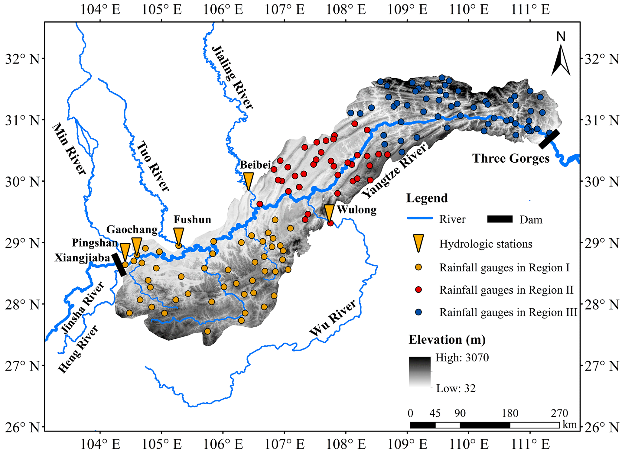
Figure 1 Schematic diagram of the interval basin between the Xiangjiaba and TGR dam sites, which is divided into three sub-regions.

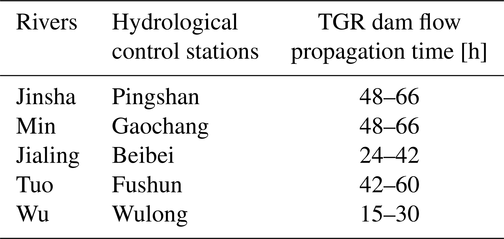
Table 1 shows the flow propagation time from the hydrological control stations of the mainstream and tributaries to the TGR dam. The outflow discharge of Xiangjiaba Reservoir, located on the Jinsha River, is observed at the Pingshan hydrological station and represents the mainstream flow. The discharge values from large tributaries (Min, Jialing, Tuo, and Wu rivers) are observed at the Gaochang, Fushun, Beibei, and Wulong hydrological stations, respectively.

Table 1 List of flow propagation time for hydrological control stations to the TGR dam site.

Considering the uneven distribution of rainfall intensity because of the narrow and long basin, the interval basin between the Xiangjiaba and TGR dam sites is divided into three sub-basins: Pingshan–Cuntan, Cuntan–Wanxian, and Wanxian–TGR dam site. Their watershed areas are 76 900, 22 900, and 27 600 km², respectively. Meanwhile, there are 45, 38, and 60 gauged rainfall stations in these three sub-regions, respectively.

2.2 Study materials

This study collects 6 h observed flow discharges at the TGR dam site and five hydrological stations (Table 1) and 6 h observed rainfall in the interval basin during the 2010–2021 flood season (May–September). The Thiessen polygon method is used to calculate areal average rainfall using rainfall station data for each sub-basin area. Meanwhile, this study collects the forecasted precipitation data issued by the European Centre for Medium-Range Weather Forecasts (ECMWF) and the Hydrology Bureau of the Yangtze River Water Resources Commission (HBYRWRC) for the 2017–2021 flood season in the three sub-basins. Their forecast time starts at 08:00 LT, with the 6–168 h forecast horizons and the 6 h forecast interval. The spatial resolution of each grid for the ECMWF forecasted precipitation is 0.125°×0.125°. The HBYRWRC forecasted precipitation is the areal average forecasted precipitation data.

The training period is from 2010 to 2016, and the validation period is from 2017 to 2021. Since the precipitation forecast starts at 08:00 LT, the forecasted flow for the 6–168 h forecast horizons is also calculated from the 08:00 LT daily in the validation period.

3 Methods

3.1 Proposed CHUP-BMA method

3.1.1 Bayesian model averaging (BMA)

Bayesian model averaging (BMA) method's principle is as follows:

$$\begin{array}{}\text{(1)}& p(Q_{\mathrm{o}}\mathrm{|}{Q}_{\mathrm{f},\mathrm{1}},Q_{\mathrm{f},\mathrm{2}},\mathrm{\dots },Q_{\mathrm{f},k})=\sum _{i=\mathrm{1}}^k{w}_i\cdot p\left(Q_{\mathrm{o}}\mathrm{|}{Q}_{\mathrm{f},i}\right),\end{array}$$

where p(⋅) denotes the probability density function. Q_o denotes the observed flow corresponding to the forecast moment (target value). k is the number of ensemble members. Q_f denotes the forecasted flow of ensemble members. w_i denotes the weight of the ith model. p(Q_o|Q_f,i) denotes the conditional probability density of Q_o conditional on Q_f,i, which is assumed to approximately obey a normal distribution with the expectation of ${\mathit{\mu }}_i=a_i+b_i\cdot Q_{\mathrm{f},i}$ and variance of σ_i. a_i and b_i are the bias correction coefficients obtained by the linear fitting of Q_f,i to Q_o.

Therefore, Eq. (1) can be rewritten as follows:

$$\begin{array}{}\text{(2)}& p(Q_{\mathrm{o}}\mathrm{|}{Q}_{\mathrm{f},\mathrm{1}},Q_{\mathrm{f},\mathrm{2}},\mathrm{\dots },Q_{\mathrm{f},k})=\sum _{i=\mathrm{1}}^k{w}_i\cdot N\left(Q_{\mathrm{o}}\mathrm{|}{\mathit{\mu }}_i{\mathit{\sigma }}_i\right).\end{array}$$

From Eq. (2), it can be seen that the BMA method does not consider the influence of the initial state (the actual observed flow at the start of the forecast) on the posterior distribution. When the member forecasts at different times are the same, the posterior probability distribution generated by the BMA is also the same, which lacks logical rationality.

3.1.2 Hydrological uncertainty processor (HUP)

Based on the assumption that the precipitation uncertainty is zero, the posterior distribution of Q_o conditional on Q_f,i and Q_b is as follows:

$$\begin{array}{}\text{(3)}& {\displaystyle }p(Q_{\mathrm{o}}\mathrm{|}{Q}_{\mathrm{f},i},Q_{\mathrm{b}})={\displaystyle \frac{p(Q_{\mathrm{f},i}\mathrm{|}{Q}_{\mathrm{o}},Q_{\mathrm{b}})\cdot p\left(Q_{\mathrm{o}}\mathrm{|}{Q}_{\mathrm{b}}\right)}{{\int }_{-\mathrm{\infty }}^{+\mathrm{\infty }}p(Q_{\mathrm{f},i}\mathrm{|}{Q}_{\mathrm{o}},Q_{\mathrm{b}})\cdot p\left(Q_{\mathrm{o}}\mathrm{|}{Q}_{\mathrm{b}}\right)\mathrm{d}{Q}_{\mathrm{o}}}},\end{array}$$

where p(Q_o|Q_b) is the prior density function, $p(Q_{\mathrm{f},i}\mathrm{|}{Q}_{\mathrm{o}},Q_{\mathrm{b}})$ is the likelihood density function, and $p(Q_{\mathrm{o}}\mathrm{|}{Q}_{\mathrm{f},i},Q_{\mathrm{b}})$ is the posterior density function.

The HUP method assumes that flow series transformed to normal space obey the Gaussian distribution. The cumulative distribution function is different for forecasted and observed flows. The common normal quantile transformation is key to the application of the HUP method and is significant for making the HUP method applicable to variables with any marginal distributions, heteroskedasticity, and nonlinear dependence structures (Krzysztofowicz and Kelly, 2000; Darbandsari and Coulibaly, 2021).

$$\begin{array}{}\text{(4)}& {\widehat{Q}}_{\mathrm{o}}=N^{-\mathrm{1}}\left(P\right(Q_{\mathrm{o}}\left)\right),{\widehat{Q}}_{\mathrm{f},i}=N^{-\mathrm{1}}\left(P\right(Q_{\mathrm{f},i}\left)\right),\end{array}$$

where P(⋅) denotes the probability distribution function. $N^{-\mathrm{1}}(\cdot )$ denotes the inverse function of the standard normal distribution. ${\widehat{Q}}_{\mathrm{o}}$ and ${\widehat{Q}}_{\mathrm{f},i}$ are the observed and forecasted flow transformed to the normal space, respectively.

The HUP method also assumes that the observed flow obeys the strictly stationary first-order Markov process (Krzysztofowicz and Kelly, 2000); i.e., the flows between adjacent forecast horizons obey the linear constraint after the normal transformation.

$$\begin{array}{}\text{(5)}& {\widehat{Q}}_{\mathrm{o},t}=c_t\times {\widehat{Q}}_{\mathrm{o},t-\mathrm{1}}+{\mathit{\epsilon }}_t,\end{array}$$

where ${\widehat{Q}}_{\mathrm{o},t}$ is the observed flow corresponding to the tth forecast horizon. c is the regression coefficient. ε is the residual, obeying $N(\mathrm{0},\mathrm{1}-c_t^{\mathrm{2}})$.

The prior density function expressions are as follows:

$$\begin{array}{}\text{(6)}& {\displaystyle }p\left({\widehat{Q}}_{\mathrm{o},t}\mathrm{|}{\widehat{Q}}_{\mathrm{b}}\right)={\displaystyle \frac{\mathrm{1}}{(\mathrm{1}-C_t^{\mathrm{2}}{)}^{\mathrm{0.5}}}}n\left\{{\displaystyle \frac{{\widehat{Q}}_{\mathrm{o},t}-C_t\times {\widehat{Q}}_{\mathrm{b}}}{(\mathrm{1}-C_t^{\mathrm{2}}{)}^{\mathrm{0.5}}}}\right\},C_t=\prod _{i=\mathrm{1}}^t{c}_i,\end{array}$$

where n(⋅) denotes standard normal density function and ${\widehat{Q}}_{\mathrm{b}}$ is the observed flow at the start of the forecast transformed to the normal space.

${\widehat{Q}}_{\mathrm{b}}$, ${\widehat{Q}}_{\mathrm{o}}$, and ${\widehat{Q}}_{\mathrm{f},i}$ are assumed to obey a linear relationship. The expression of the likelihood function in normal space is as follows:

$$\begin{array}{}\text{(7)}& {\displaystyle }& {\displaystyle }{\widehat{Q}}_{\mathrm{f},i,t}=a_t\times {\widehat{Q}}_{\mathrm{o},t}+d_t\times {\widehat{Q}}_{\mathrm{b}}+b_t+{\mathit{\theta }}_t,\text{(8)}& {\displaystyle }& {\displaystyle }p({\widehat{Q}}_{\mathrm{f},i,t}\mathrm{|}{\widehat{Q}}_{\mathrm{o},t},{\widehat{Q}}_{\mathrm{b}})={\displaystyle \frac{\mathrm{1}}{{\mathit{\sigma }}_t}}n\left\{{\displaystyle \frac{{\widehat{Q}}_{\mathrm{f},i,t}-(a_t\times {\widehat{Q}}_{\mathrm{o},t}+d_t\times {\widehat{Q}}_{\mathrm{b}}+b_t)}{{\mathit{\sigma }}_t}}\right\},\end{array}$$

where θ_t is an independent variable obeying $N(\mathrm{0},{\mathit{\sigma }}_t^{\mathrm{2}}$). a_t, d_t, and b_t are regression coefficients.

The posterior density function under normal space can be derived by substituting Eqs. (6) and (7) in Eq. (3):

$$\begin{array}{}\text{(9)}& \begin{array}{rl}& p({\widehat{Q}}_{\mathrm{o},t}\mathrm{|}{\widehat{Q}}_{\mathrm{f},i,t},{\widehat{Q}}_{\mathrm{b}})={\displaystyle \frac{\mathrm{1}}{Y_t}}n\left\{{\displaystyle \frac{{\widehat{Q}}_{\mathrm{o},t}-(A_t\times {\widehat{Q}}_{\mathrm{f},i,t}+D_t\times {\widehat{Q}}_{\mathrm{b}}+B_t)}{Y_t}}\right\},\\ & A_t={\displaystyle \frac{a_t{y}_t^{\mathrm{2}}}{a_t^{\mathrm{2}}{y}_t^{\mathrm{2}}+{\mathit{\sigma }}_t^{\mathrm{2}}}},B_t={\displaystyle \frac{-a_t{b}_t{y}_t^{\mathrm{2}}}{a_t^{\mathrm{2}}{y}_t^{\mathrm{2}}+{\mathit{\sigma }}_t^{\mathrm{2}}}},\\ & D_t={\displaystyle \frac{C_t{\mathit{\sigma }}_t^{\mathrm{2}}-a_t{d}_t{y}_t^{\mathrm{2}}}{a_t^{\mathrm{2}}{y}_t^{\mathrm{2}}+{\mathit{\sigma }}_t^{\mathrm{2}}}},Y_t={\left({\displaystyle \frac{y_t^{\mathrm{2}}{\mathit{\sigma }}_t^{\mathrm{2}}}{a_t^{\mathrm{2}}{y}_t^{\mathrm{2}}+{\mathit{\sigma }}_t^{\mathrm{2}}}}\right)}^{\mathrm{0.5}},\\ & y_t^{\mathrm{2}}=\mathrm{1}-C_t^{\mathrm{2}}.\end{array}\end{array}$$

The posterior distribution function under the normal space can be converted to the original space by Jacobian transformation (Liu et al., 2016). The posterior density function of Q_o,t under $Q_{\mathrm{f},i,t}$ and Q_b conditions is as follows:

$$\begin{array}{}\text{(10)}& \begin{array}{rl}p(Q_{\mathrm{o},t}\mathrm{|}& Q_{\mathrm{f},i,t},Q_{\mathrm{b}})={\displaystyle \frac{J\left(Q_{\mathrm{o},t}\right)}{Y_t}}n\\ & \left\{{\displaystyle \frac{\left\{\begin{array}{c}{N}^{-\mathrm{1}}\left(P\right(Q_{\mathrm{o},t}\left)\right)\\ -A_t{N}^{-\mathrm{1}}\left(P\right(Q_{\mathrm{f},i,t}\left)\right)\\ -D_t{N}^{-\mathrm{1}}\left(P\right(Q_{\mathrm{b}}\left)\right)-B_t\end{array}\right\}}{Y_t}}\right\},\\ & J\left(Q_{\mathrm{o},t}\right)={\displaystyle \frac{p\left(Q_{\mathrm{o},t}\right)}{n\left(N^{-\mathrm{1}}\right(P\left(Q_{\mathrm{o},t}\right)\left)\right)}},\end{array}\end{array}$$

where J(⋅) is the Jacobian transformation function.

3.1.3 HUP-BMA method

Darbandsari and Coulibaly et al. (2021) applied the hydrological uncertainty processor (HUP) to the ensemble forecast members, substituted the posterior density function obtained by the HUP method (Eq. 9) in the BMA framework (Eq. 2), and then obtained the posterior distribution function of the target flow based on the initial state and the forecasted flow of the ensemble member. Therefore, the expression of the HUP-BMA method is as follows:

$$\begin{array}{}\text{(11)}& \begin{array}{rl}p(Q_{\mathrm{o}}\mathrm{|}& Q_{\mathrm{f},\mathrm{1}},Q_{\mathrm{f},\mathrm{2}},\mathrm{\dots },Q_{\mathrm{f},k},Q_{\mathrm{b}})=\sum _{i=\mathrm{1}}^k{w}_i\cdot {\displaystyle \frac{J\left(Q_{\mathrm{o},t}\right)}{Y_t}}\\ & n\left\{{\displaystyle \frac{\left\{\begin{array}{c}{N}^{-\mathrm{1}}\left(P\right(Q_{\mathrm{o},t}\left)\right)\\ -A_t{N}^{-\mathrm{1}}\left(P\right(Q_{\mathrm{f},i,t}\left)\right)\\ -D_t{N}^{-\mathrm{1}}\left(P\right(Q_{\mathrm{b}}\left)\right)-B_t\end{array}\right\}}{Y_t}}\right\}.\end{array}\end{array}$$

3.1.4 Copula-based HUP-BMA (CHUP-BMA) method

Copula-based HUP

According to Sklar's theorem (Sklar, 1959), the joint distribution of m variables is as follows:

$$\begin{array}{}\text{(12)}& P(x_{\mathrm{1}},x_{\mathrm{2}},\mathrm{\dots }\mathrm{\dots },x_m)=C_m\left(P\right(x_{\mathrm{1}}),P(x_{\mathrm{2}}),\mathrm{\dots }\mathrm{\dots },P(x_m\left)\right),\end{array}$$

where C_m(⋅) denotes the m-dimensional copula distribution.

The copula-based HUP method (CHUP), which can avoid the normal quantile transformation process of the flow series in the standard HUP method, was proposed by Liu et al. (2018). With the help of the copula function, the prior density function in Eq. (3) can be derived as follows:

$$\begin{array}{}\text{(13)}& {\displaystyle }\begin{array}{rl}{\displaystyle }p\left(Q_{\mathrm{o}}\mathrm{|}{Q}_{\mathrm{b}}\right)& {\displaystyle }={\displaystyle \frac{{\partial }^{\mathrm{2}}{C}_{\mathrm{2}}\left(P\right(Q_{\mathrm{o}}),P(Q_{\mathrm{b}}\left)\right)}{\partial P\left(Q_{\mathrm{o}}\right)\partial P\left(Q_{\mathrm{b}}\right)}}\cdot {\displaystyle \frac{\mathrm{d}P\left(Q_{\mathrm{o}}\right)}{\mathrm{d}{Q}_{\mathrm{o}}}}\\ {\displaystyle }& {\displaystyle }=c_{\mathrm{2}}\left(P\right(Q_{\mathrm{o}}),P(Q_{\mathrm{b}}\left)\right)\cdot p\left(Q_{\mathrm{o}}\right),\end{array}\end{array}$$

where c_m(⋅) denotes the m-dimensional copula density function. m denotes the dimension.

The likelihood density function in Eq. (3) can be derived as follows:

$$\begin{array}{}\text{(14)}& \begin{array}{rl}p(Q_{\mathrm{f},i}\mathrm{|}{Q}_{\mathrm{o}},Q_{\mathrm{b}})& ={\displaystyle \frac{{\displaystyle \frac{{\partial }^{\mathrm{3}}{C}_{\mathrm{3}}\left(P\right(Q_{\mathrm{o}}),P(Q_{\mathrm{f},i}),P(Q_{\mathrm{b}}\left)\right)}{\partial P\left(Q_{\mathrm{o}}\right)\cdot \partial P\left(Q_{\mathrm{f},i}\right)\cdot \partial P\left(Q_{\mathrm{b}}\right)}}}{{\displaystyle \frac{{\partial }^{\mathrm{2}}{C}_{\mathrm{2}}\left(P\right(Q_{\mathrm{o}}),P(Q_{\mathrm{b}}\left)\right)}{\partial P\left(Q_{\mathrm{o}}\right)\cdot \partial P\left(Q_{\mathrm{b}}\right)}}}}\\ & \cdot {\displaystyle \frac{\mathrm{d}P\left(Q_{\mathrm{f},i}\right)}{\mathrm{d}{Q}_{\mathrm{f},i}}}={\displaystyle \frac{c_{\mathrm{3}}\left(P\right(Q_{\mathrm{o}}),P(Q_{\mathrm{f},i}),P(Q_{\mathrm{b}}\left)\right)}{c_{\mathrm{2}}\left(P\right(Q_{\mathrm{o}}),P(Q_{\mathrm{b}}\left)\right)}}\\ & \cdot p\left(Q_{\mathrm{f},i}\right).\end{array}\end{array}$$

The posterior density function in Eq. (3) can be derived as follows:

$$\begin{array}{}\text{(15)}& \begin{array}{rl}p(Q_{\mathrm{o}}\mathrm{|}{Q}_{\mathrm{f},i},Q_{\mathrm{b}})& ={\displaystyle \frac{c_{\mathrm{3}}\left(P\right(Q_{\mathrm{o}}),P(Q_{\mathrm{f},i}),P(Q_{\mathrm{b}}\left)\right)}{{\int }_{\mathrm{0}}^{\mathrm{1}}{c}_{\mathrm{3}}\left(P\right(Q_{\mathrm{o}}),P(Q_{\mathrm{f},i}),P(Q_{\mathrm{b}}\left)\right)\mathrm{d}P\left(Q_{\mathrm{o}}\right)}}\\ & \cdot p\left(Q_{\mathrm{o}}\right).\end{array}\end{array}$$

Copula-based HUP-BMA method

Applying CHUP to the ith ensemble member, the posterior probability distribution function $p(Q_{\mathrm{o}}\mathrm{|}{Q}_{\mathrm{f},i},Q_{\mathrm{b}})$ of Q_o based on Q_f,i and Q_b can be obtained. Coupling $p(Q_{\mathrm{o}}\mathrm{|}{Q}_{\mathrm{f},i},Q_{\mathrm{b}})$ with the BMA framework, the copula-based HUP-BMA (CHUP-BMA) method can be constructed and Eq. (2) can become as follows:

$$\begin{array}{}\text{(16)}& {\displaystyle }\begin{array}{rl}{\displaystyle }p(& {\displaystyle }{Q}_{\mathrm{o}}\mathrm{|}{Q}_{\mathrm{f},\mathrm{1}},Q_{\mathrm{f},\mathrm{2}},\mathrm{\dots },Q_{\mathrm{f},k},Q_{\mathrm{b}})={\sum }_{i=\mathrm{1}}^k{w}_i\\ {\displaystyle }& {\displaystyle }\cdot {\displaystyle \frac{c_{\mathrm{3}}\left(P\right(Q_{\mathrm{o}}),P(Q_{\mathrm{f},i}),P(Q_{\mathrm{b}}\left)\right)}{{\int }_{\mathrm{0}}^{\mathrm{1}}{c}_{\mathrm{3}}\left(P\right(Q_{\mathrm{o}}),P(Q_{\mathrm{f},i}),P(Q_{\mathrm{b}}\left)\right)\mathrm{d}P\left(Q_{\mathrm{o}}\right)}}\cdot p\left(Q_{\mathrm{o}}\right).\end{array}\end{array}$$

The forecast uncertainty is quantified by the forecast interval with a 90 % confidence level. Before constructing the copula, selecting the marginal distribution and the copula type is usually necessary. This study intends to select the appropriate marginal distribution and copula function from five common distribution functions, such as Pearson type III (P-III), gamma, normal, lognormal, and Weibull, and five common copula functions, such as the Gumbel–Hougaard, Frank, Clayton, Student t (Student), and Gaussian copulas, according to the root mean square error (RMSE) minimization criterion, respectively. For the definition and mathematical expressions of copula functions, refer to Liu et al. (2018) and Chen and Guo (2019).

Darbandsari and Coulibaly (2021) demonstrated that the HUP-BMA method could improve the probabilistic forecasting performance of the HUP and BMA methods in the short forecast horizons. Therefore, this paper focuses on analyzing and comparing the performance of the HUP-BMA and CHUP-BMA methods. The HUP-BMA and CHUP-BMA methods only calibrate the ensemble members' weights through the expectation–maximization (EM) algorithm (Darbandsari and Coulibaly, 2021). Meanwhile, since the forecast accuracy of ensemble members may change with time due to seasonality and other factors (Zhong et al., 2020), the sliding window approach is used to update the weighting parameters. Parrish et al. (2012) and Darbandsari and Coulibaly (2020) have shown that the BMA method with the sliding window can obtain better probabilistic forecast performance compared to the method without the sliding window.

3.2 Ensemble forecasting scheme

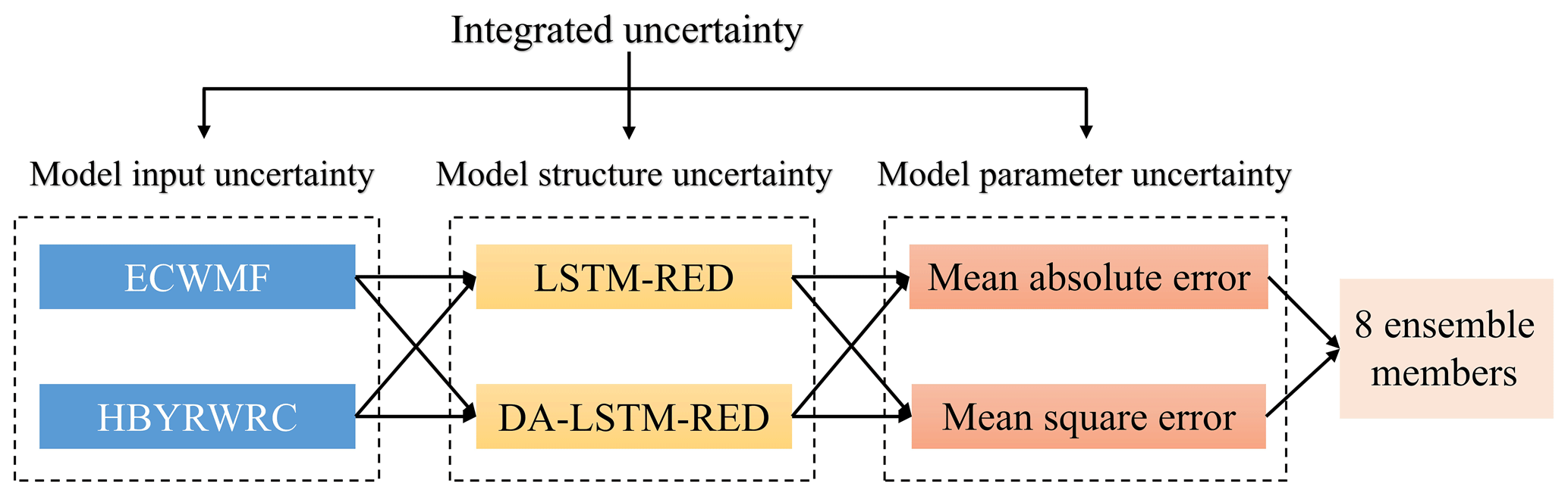
An ensemble forecast scheme containing multi-source uncertainties in the model input, the model structure, and the parameter is constructed using a multi-member approach consisting of two forecasted precipitations, two models, and two objective functions used to calibrate parameters, as shown in Fig. 2.

Figure 2 The TGR's flood ensemble forecast scheme.

3.2.1 Model input uncertainty

There are five flow discharge inputs from five large tributaries (Jinsha, Min, Jialing, Tuo, and Wu rivers) in our case study. The flow discharges are observed at the Pingshan, Gaochang, Fushun, Beibei, and Wulong controlled hydrological stations, respectively. Since these observed (or forecasted) flows are regulated by their respective upstream cascade reservoirs, these flow data inputs are more accurate than the rainfall inputs. This study collected the forecasted precipitation data from the European Centre for Medium-Range Weather Forecasts (ECMWF) and HBYRWRC in these three sub-basins. Since the rainfall data are more diverse and have relatively large uncertainty, the forecast rainfall input variable is used to explore the impact of forecast rainfall uncertainty on the TGR inflow forecasts. The TGR is a river-type reservoir, so building a river confluence model for flood forecasting is necessary. The observed and forecasted precipitations are converted into the effective precipitation in the three sub-basin areas, which accounts for the losses of plant reception, infiltration, evaporation, etc. The rainfall–runoff relationship (Fedora and Beschta, 1989) is commonly used in the Yangtze River basin to calculate the effective precipitation. The antecedent precipitation index, which is the key variable of the method, can be calculated by the following equation to represent the soil moisture content (Zhong et al., 2018b):

$$\begin{array}{}\text{(17)}& {\displaystyle }{P}_{\mathrm{a},t+\mathrm{1}}=k(P_{\mathrm{a},t}+P_t),\text{(18)}& {\displaystyle }{P}_{\mathrm{a},t+\mathrm{1}}\le I_m,\end{array}$$

where P_a,t denotes the antecedent precipitation index on the tth day, P_t is the daily precipitation, I_m is the water storage capacity of the basin, and k denotes evaporation reduction index.

The values of k and I_m for these three sub-basins are listed in Table 2, which are obtained from the HBYRWRC. Since the rainfall–runoff relationship graph method has been widely used for runoff generation calculation in the Yangtze River basin, the rainfall–runoff relationship between the Xiangjiaba and Three Gorges dam sites uncontrolled interval basin is established and plotted in Fig. 3 and is used to calculate the effective precipitation based on the antecedent precipitation index (P_a) and observed (or forecasted) precipitation for these three sub-basins.

Table 2 The k and I_m values for the three sub-basin areas.

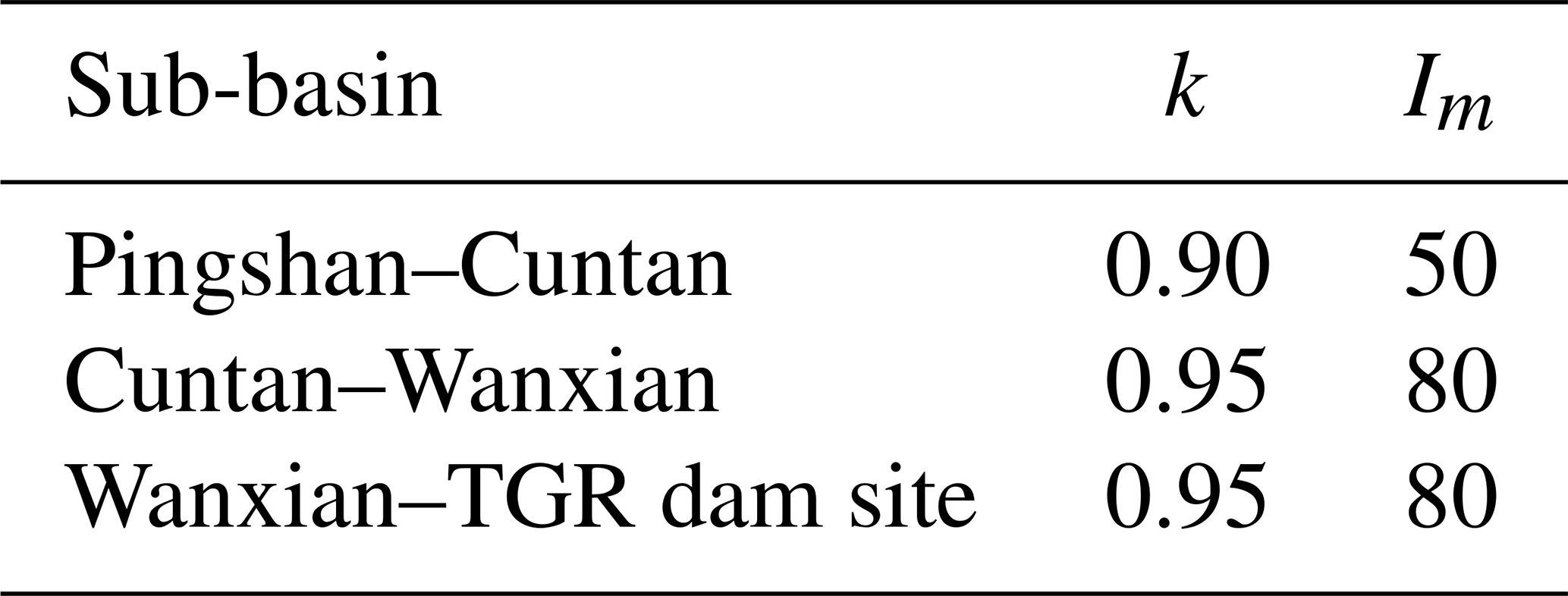
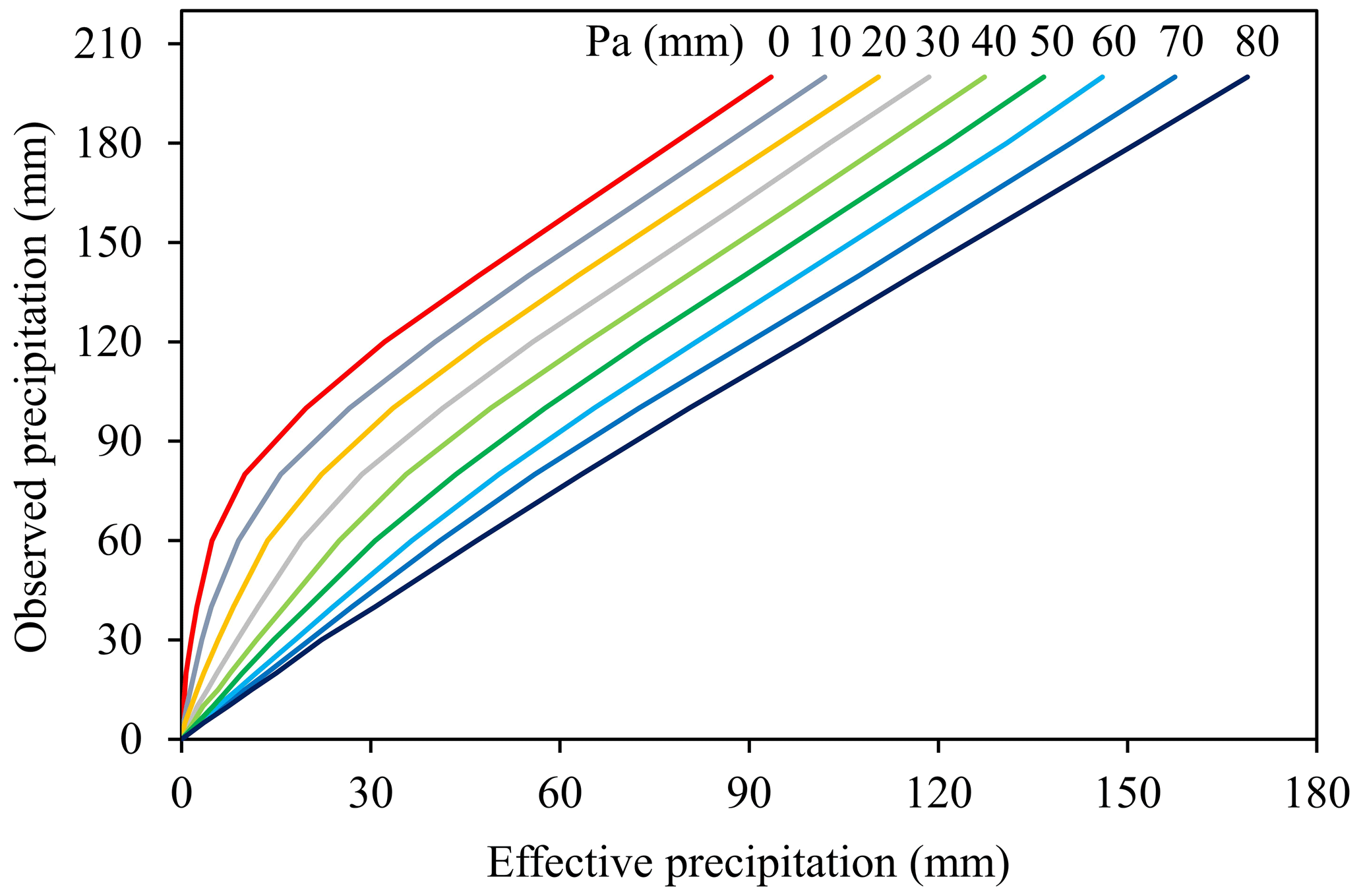
Figure 3 Rainfall–runoff relationship between the Xiangjiaba and Three Gorges dam sites' uncontrolled interval basin.

After obtaining the daily antecedent precipitation index at 08:00 LT, the antecedent precipitation index for the 6 h timescale is calculated as follows:

$$\begin{array}{}\text{(19)}& P_{\mathrm{a},t,m}=(P_{\mathrm{a},t}+\sum P_{t,n})\times k^{\frac{h}{\mathrm{24}}},\end{array}$$

where $P_{\mathrm{a},t,m}$ denotes the antecedent precipitation index at m:00 LT on the tth day. $\sum P_{t,n}$ denotes the cumulative observed precipitation from 08:00 to m:00 LT on the tth day. h denotes the time gap from 08:00 to m:00 LT on the tth day.

3.2.2 Model structure uncertainty

The TGR inflow forecasting is influenced by the upstream mainstream and tributary reservoir scheduling decisions, the rainfall intensity and distribution in the interval basin, and the changes in the subsurface characteristics, which is challenging to establish complex and physically based hydrological models (Yang et al., 2019; Cho and Kim, 2022; Hauswirth et al., 2023). The simulation or forecast accuracy in this interval basin needs to be improved to meet the needs of the work. Therefore, two advanced data-driven models for obtaining multi-step-ahead flood processes forecasting, namely the long short-term memory model based on a recursive encoder–decoder structure (LSTM-RED) and the coupled dual attention LSTM-RED (DA-LSTM-RED) model, are used for confluence calculations as a way to consider the uncertainty in the model structure. Since the forecast data series at the outlets of tributaries are inconsistent, the observed flow at the outlets of five large tributaries is used to train and validate the proposed models.

Long short-term memory model based on encoder–decoder structure

The structure of the LSTM neural network includes the forgetting gate, input gate, updating the state of the memory unit, and output gate (Hochreiter and Schmidhuber, 1997). The forgetting gate can select the relatively important information in the previous memory unit. The input gate can select useful information from the input variables in the current moment. The memory unit state can store relatively important information extracted from historical moments, which is updated under the control of the forgetting gate and the input gate. The output gate selects and outputs useful information from the memory cell state. More detailed procedures of the LSTM neural network formulation have been described by Kratzert et al. (2018).

This study nests an LSTM neural network into a recursive encoder–decoder (RED) structure that can be obtained for forecasting flood processes to build an LSTM-RED model. Among them, the RED structure is similar to that of Kao et al. (2020). The description of the LSTM neural network can be found in Cui et al. (2022). The encoding process of the RED structure is used to extract the critical information (C_t) of the input (Xiang et al., 2020). In the decoding process, forecast information of the same category as the encoding process is another input to the neural network of the latter moment apart from the C_t and the output of the hidden layer in the previous moment.

LSTM-RED neural network coupled dual attention mechanism

The LSTM-RED model based on the dual attention mechanism (DA-LSTM-RED) is established by adding the feature–temporal dual attention mechanism to the LSTM-RED model, which can enable the model to highlight effective information in different types and moments of the input. The DA mechanism (Fig. 4) consists of the feature attention module, the temporal attention module, and the forecast input processing module.

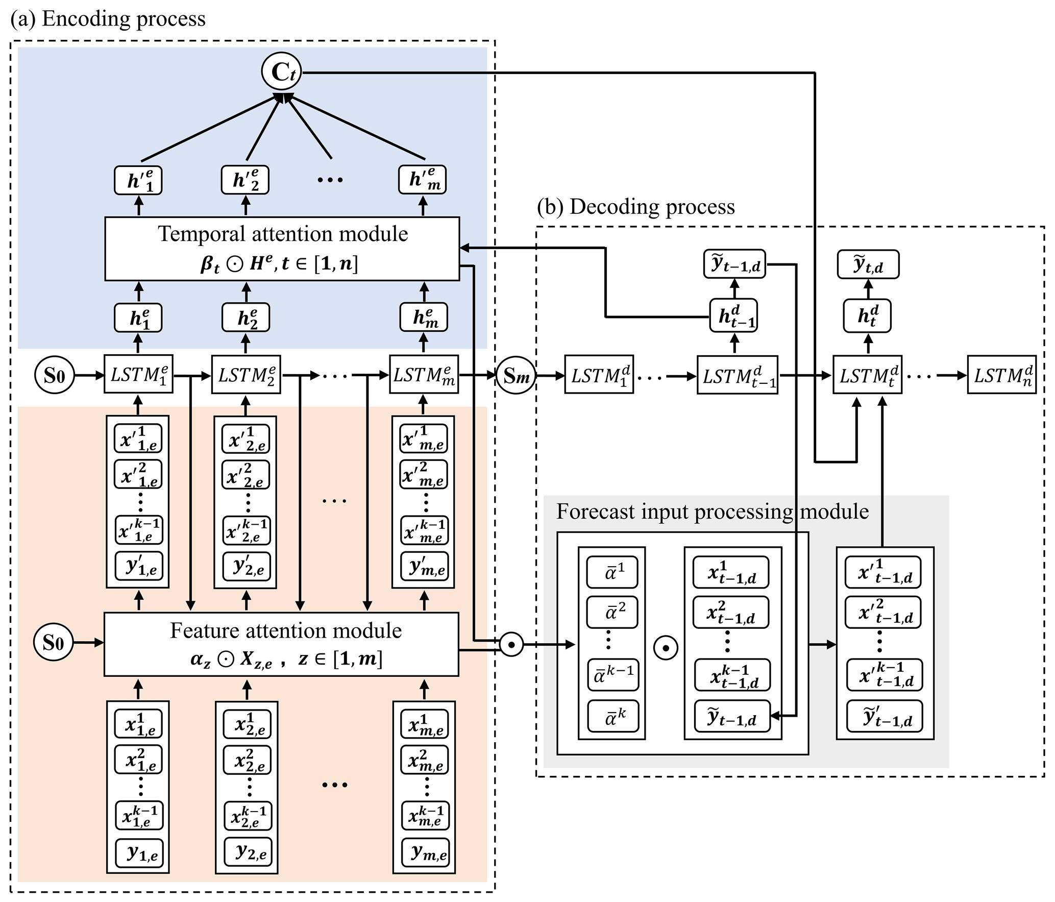
Figure 4 Schematic diagram of the DA-LSTM-RED model. Illustrations a and b are the encoding and decoding processes, respectively. k is the number of input types. X_z,e is the input variable of encoding process; ${\mathit{X}}_{\mathbf{z},\mathbf{e}}=\mathit{\{}{x}_{z,e}^{\mathrm{1}},x_{z,e}^{\mathrm{2}},\mathrm{\dots },x_{z,e}^{k-\mathrm{1}},y_{z,e}\mathit{\}}$. α_z denotes the weights of the input variables; ${\mathit{\alpha }}_{\mathbf{z}}=\mathit{\{}{\mathit{\alpha }}_z^{\mathrm{1}},{\mathit{\alpha }}_z^{\mathrm{2}}\mathrm{\dots },{\mathit{\alpha }}_z^k\mathit{\}}$. m is the input time steps in the encoding process. S is the hidden layer output. n is the maximum forecast horizon. H^e is the hidden layer state; ${\mathit{H}}^{\mathit{e}}=\mathit{\{}{h}_{\mathrm{1}}^e,h_{\mathrm{2}}^e,\mathrm{\dots },h_m^e\mathit{\}}$. β_t denotes the weights of the hidden layer states of the encoding process; ${\mathit{\beta }}_{\mathit{t}}=\mathit{\{}{\mathit{\beta }}_t^{\mathrm{1}},{\mathit{\beta }}_t^{\mathrm{2}},\mathrm{\dots },{\mathit{\beta }}_t^m\mathit{\}}$. C denotes the key information highlighted by the temporal attention. $\stackrel{\mathrm{‾}}{\mathit{\alpha }}$ denotes the forecast input weights.

The feature attention module can adaptively highlight the critical input types by assigning feature weights to the input of the encoding process (Qin et al., 2017). The temporal attention module can highlight the information (hidden layer states) extracted at a critical time step by assigning temporal weights to the information extracted at all time steps in the encoding process (Ding et al., 2020). Meanwhile, the feature weights are averaged based on temporal weights and applied to the forecast information inputted in the decoding process, thus highlighting the key forecast input variables. The principle of the DA-LSTM-RED model can be found in Cui et al. (2023).

Model input and hyperparameter selection

In this study, the input types for the encoding process include effective precipitation in the three sub-basins, flow discharge in the mainstream and tributaries (i.e., five hydrological stations in Table 1), and previously observed inflow to the TGR for a total of nine data types. In order to make the model learn comprehensive information, input variables with the last 11 time steps (66 h) are inputted to the encoding process according to the flow propagation times from the hydrological stations to the TGR dam site in Table 1.

The forecasted effective precipitation, the forecasted flow of the mainstream and tributaries, and the forecasted flow for the previous forecast horizon are used as inputs to the decoding process. Among them, the forecasted effective precipitation is calculated by the observed precipitation during the training period and by the forecast precipitation during the validation period. The forecasted flow of the upstream mainstream and tributaries is replaced by the observed flow during the training and validation periods. The TGR's observed inflow for the 6–168 h forecast horizons is the target output, which is needed for practical forecasting.

The input and output data are handled by the normalization method. Moreover, the trial-and-error method is used for debugging the network hyperparameters. The model is trained by the Adam method (Kingma and Ba, 2014).

3.2.3 Model parameter uncertainty

Different parameter optimization objective functions may focus on different forecast results (Zhong et al., 2020). For example, the mean absolute error function focuses on the magnitude of the error mean. The mean square error function is usually sensitive to outliers with large errors, which may make the model parameters with different objective functions produce forecast results with different focus points (Duan et al., 2007). Therefore, it is necessary to consider the uncertainty of the model parameters. Neural network models usually train model parameters (such as model internal weights and bias values) based on loss functions, so this paper uses two common loss functions, namely the mean absolute error and the mean square error, to train the model as a way of considering the uncertainty of model parameters.

3.3 Evaluation metrics

3.3.1 Deterministic forecast evaluation metrics

The accuracy of deterministic forecast is evaluated by three metrics: the Nash–Sutcliffe efficiency (NSE; Nash and Sutcliffe, 1970), the mean absolute error (MAE), and the relative error in total runoff (RE).

$$\begin{array}{}\text{(20)}& {\displaystyle }\text{NSE}=\mathrm{1}-{\displaystyle \frac{{\sum }_{i=\mathrm{1}}^N(Q_{\mathrm{o},i}-Q_{\mathrm{f},i}{)}^{\mathrm{2}}}{{\sum }_{i=\mathrm{1}}^N(Q_{\mathrm{o},i}-\stackrel{\mathrm{‾}}{Q_{\mathrm{o}}}{)}^{\mathrm{2}}}},\text{(21)}& {\displaystyle }\text{RE}={\displaystyle \frac{{\sum }_{i=\mathrm{1}}^N{Q}_{\mathrm{f},i}-{\sum }_{i=\mathrm{1}}^N{Q}_{\mathrm{o},i}}{{\sum }_{i=\mathrm{1}}^N{Q}_{\mathrm{o},i}}}\times \mathrm{100}\mathit{\%},\text{(22)}& {\displaystyle }\text{MAE}={\displaystyle \frac{\mathrm{1}}{N}}\sum _{i=\mathrm{1}}^N|Q_{\mathrm{o},i}-Q_{\mathrm{f},i}|,\end{array}$$

where N is the sample number and $\stackrel{\mathrm{‾}}{Q_{\mathrm{o}}}$ and $\stackrel{\mathrm{‾}}{Q_{\mathrm{f}}}$ are the average of the observed and forecasted flow, respectively.

The Nash–Sutcliffe efficiency (NSE) is one of the most important metrics in flood forecasting, reflecting the degree of fit between forecasted and observed flows (Nash and Sutcliffe, 1970). Since the accurate runoff volume predictions are more important than peak discharge for the operation of a large reservoir (Cui et al., 2023), the relative error for total runoff volume (RE) is also chosen. The mean absolute error (MAE) can reflect the forecast error for each moment and is compared with the continuous ranked probability score (CRPS) of the ensemble forecast (Raftery et al., 2005), which can reflect the effectiveness of the ensemble forecast correction.

3.3.2 Probabilistic forecast evaluation metrics

Forecast interval evaluation metrics

The forecast interval is evaluated by three metrics: the average coverage rate (CR), the average interval width (IW), and the percentage of observations bracketed by the unit confidence interval (PUCI; Li et al., 2011).

$$\begin{array}{}\text{(23)}& {\displaystyle }\text{CR}={\displaystyle \frac{n_c}{N}},\text{(24)}& {\displaystyle }\text{IW}={\displaystyle \frac{\mathrm{1}}{N}}\sum _{i=\mathrm{1}}^N(Q_{\mathrm{u},i}-Q_{\mathrm{l},i}),\text{(25)}& {\displaystyle }\text{PUCI}={\displaystyle \frac{\text{CR}}{\frac{\mathrm{1}}{N}{\sum }_{i=\mathrm{1}}^N\left(\frac{Q_{\mathrm{u},i}-Q_{\mathrm{l},i}}{Q_{\mathrm{o},i}}\right)}},\end{array}$$

where n_c denotes the number of values of Q_o located in the forecast interval. Q_u and Q_l are the upper and lower boundaries of the forecast interval, respectively, with a 90 % confidence level.

The average coverage rate (CR) is one of the most necessary metrics for evaluating the reliability of forecast intervals (Li et al., 2021). The average interval width (IW) is the metric that directly reflects the level of forecast uncertainty, which is an important metric for evaluating the effectiveness of the proposed methods. The percentage of observations bracketed by the unit confidence interval (PUCI) is a comprehensive metric for evaluating the performance of forecast intervals in quantifying uncertainty (Xiong et al., 2009). Therefore, the CR, RB, and PUCI metrics are selected to evaluate the forecast intervals performance.

Probabilistic forecast evaluation metrics

The probabilistic forecast is evaluated by three metrics: the α_index (Renard et al., 2010), the ignorance score (IGS) (Gneiting et al., 2005), and the continuous ranked probability score (CRPS) (Raftery et al., 2005).

$$\begin{array}{c}\text{(26)}& {\displaystyle }\mathit{\alpha }\mathit{\_}\text{index}=\mathrm{1}-{\displaystyle \frac{\mathrm{2}}{N}}\sum _{i=\mathrm{1}}^N|q_{\mathrm{e},i}-q_{\text{th},i}|,\text{(27)}& {\displaystyle }\text{IGS}=-{\displaystyle \frac{\mathrm{1}}{N}}\sum _{i=\mathrm{1}}^N\ln \left(p\right(Q_{\mathrm{o},i}\left)\right),\text{(28)}& {\displaystyle }\text{CRPS}={\displaystyle \frac{\mathrm{1}}{N}}\sum _{i=\mathrm{1}}^N\underset{\mathrm{0}}{\overset{+\mathrm{\infty }}{\int }}\left(P_i\right(r)-I(r-Q_{\mathrm{o},i}){)}^{\mathrm{2}}\mathrm{d}r,{\displaystyle }I(r-Q_{\mathrm{o},i})=\left\{\begin{array}{ll}\mathrm{1},& r\ge Q_{\mathrm{o},i},\\ \mathrm{0},& r<Q_{\mathrm{o},i},\end{array}\right.\end{array}$$

where, q_e,i and q_th,i denote the observed and theoretical p values of Q_o,i, respectively. The p value denotes the posterior probability distribution value of the Q_o,i (Renard et al., 2010). I(⋅) denotes the indicator function. r denotes the flow variable.

The α_index metric can quantitatively assess the reliability of ensemble probabilistic forecasts from the perspective of distribution function values (Renard et al., 2010). The closer the α_index value is to 1, the more reliable the probabilistic forecast. The IGS and CRPS metrics can reflect the reliability and sharpness of the probabilistic forecast. The former can quantify the forecast probability density at the observation, while the latter can indicate the fit performance between the posterior probabilistic distribution and the actual probabilistic distribution of Q_o (Raftery et al., 2005). Both CRPS and IGS are negative scores; i.e., the smaller the value, the better. The IGS imposes severe penalties for particularly poor probabilistic predictions and may be extremely sensitive to outliers and extreme events, yet it also lacks robustness (Raftery et al., 2005).

4 Result evaluation

4.1 Deterministic forecast results of ensemble members

Since the study focuses on the differences in ensemble forecast performance between the HUP-BMA and CHUP-BMA methods, the overall forecast accuracy of members is analyzed (Fig. 5) and the differences in forecast accuracy between members are not explicitly analyzed. As shown in Fig. 5, using the observed values as input during the training period, high forecast accuracy can be acquired in different forecast horizons, with the NSE values exceeding 0.95, the MAE values being below 1400 m³ s⁻¹, and the absolute value of RE staying within 4 %.

Figure 5 Statistical chart of evaluation metrics of eight ensemble members.

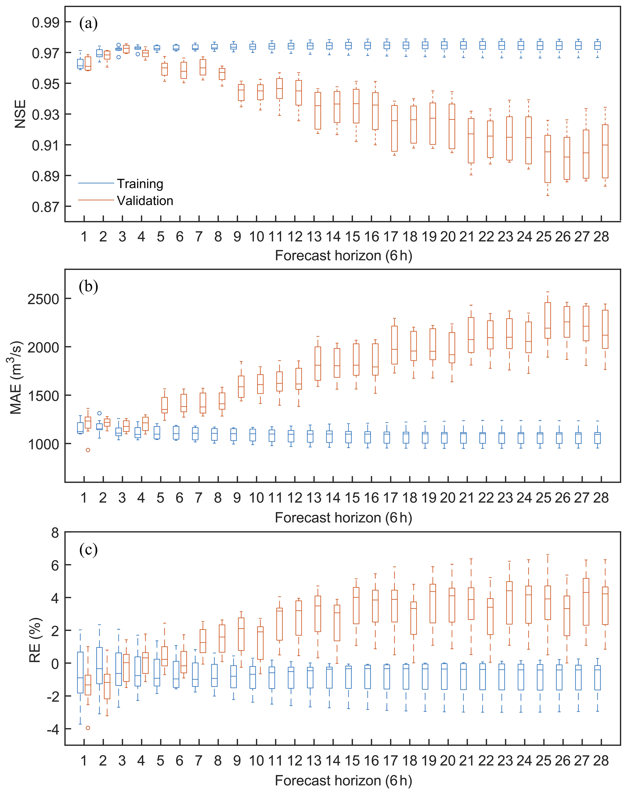
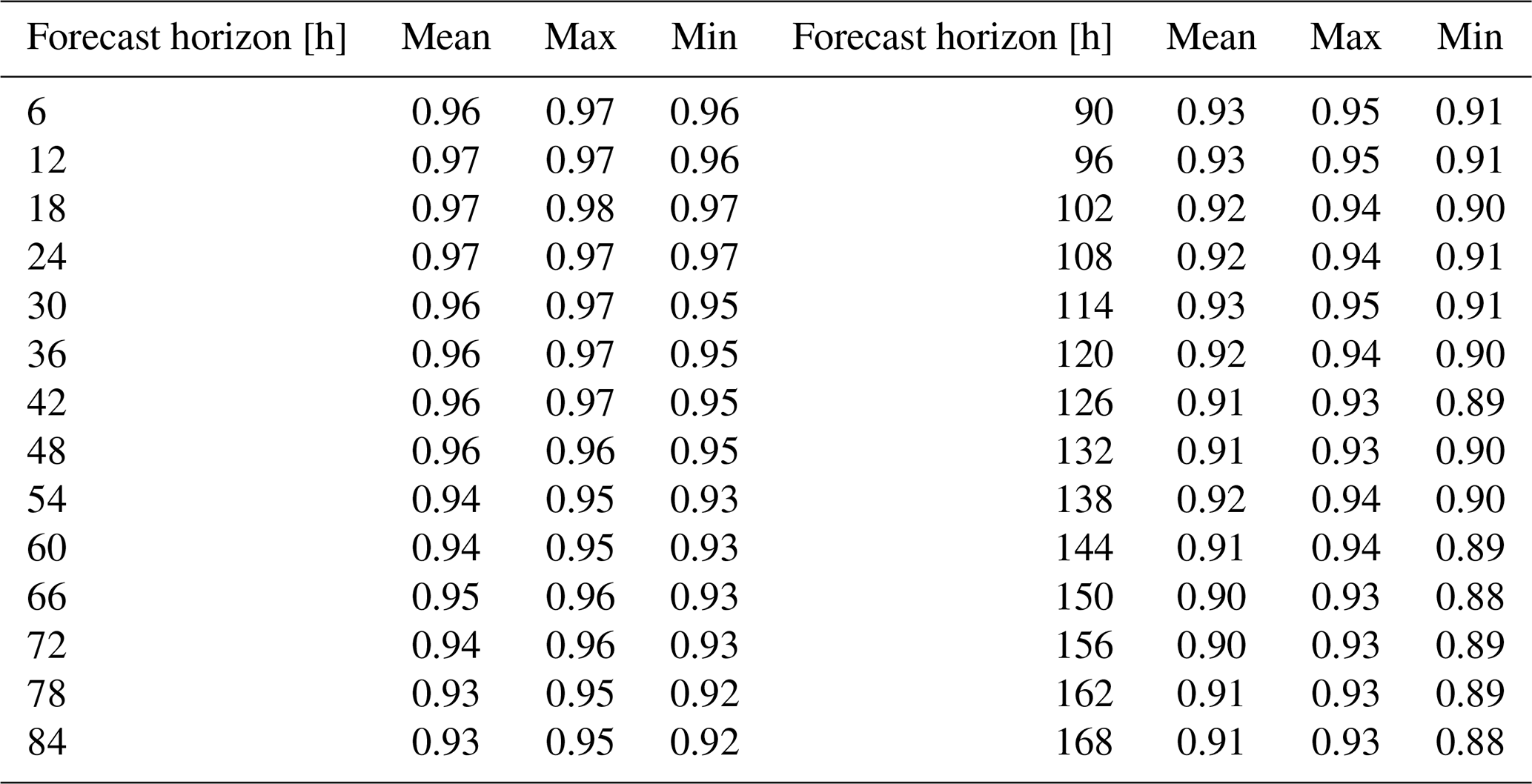
After combining the forecasted precipitation during the validation period, the NSE values show a decreasing trend and the MAE and RE values show an increasing trend with the increase in the forecast horizon. Taking the NSE metrics of the 1–7 d forecast horizons as an example (Table 3), the average value of the NSE metric decreases from 0.97 to 0.89, which indicates that the forecast accuracy gradually decreases. Meanwhile, the range of evaluation metrics gradually increases with the increase in the forecast horizon. It can be seen from Table 3 that the difference between the maximum and minimum values of NSE indicators for the 1 d forecast horizon is only 0.01. In contrast, the difference for the 7 d forecast horizon is as high as 0.05, which indicates that the difference in forecast accuracy of members is also more significant and that the forecast uncertainty gradually increases. Overall, the NSE values of the forecast members in the 6–168 h forecast horizons are higher than 0.88, and the absolute values of the RE metrics are within 7 %. Hence, the forecast accuracy of members is relatively high and the forecast error is low, which can be used for flood ensemble forecasting.

Table 3 Mean, minimum, and maximum values of NSE metrics for eight ensemble members in the validation period.

4.2 Ensemble forecast results

4.2.1 Marginal distribution and copula function selection

It is necessary to first fit the marginal distributions of the observed flow and the forecasted flow of the 6–168 h forecast horizons. The Q_o and Q_b obey the same distribution. The RMSE criterion is used to select the marginal distribution type. In each forecast horizon, the RMSE values of the eight members are averaged to obtain the marginal distribution suitable for the forecasted flow intuitively. Meanwhile, according to Eq. (14), the three-dimensional joint distribution of Q_o, Q_b, and Q_f needs to be constructed. The RMSE criterion is used to select the copula function. Similarly, the RMSE values for the eight members of each forecast horizon were averaged.

Figure 6a and b show the RMSE values generated by fitting the marginal distribution and copula function, respectively. It can be seen from Fig. 6a that the lognormal distribution has the lowest RMSE value among the five alternative marginal distributions and is chosen as the sequence marginal distribution type. As shown in Fig. 6b, the Student copula has the lowest RMSE value in the 6–168 h forecast horizons and is chosen to construct the three-dimensional joint distribution function of Q_o, Q_b, and Q_f.

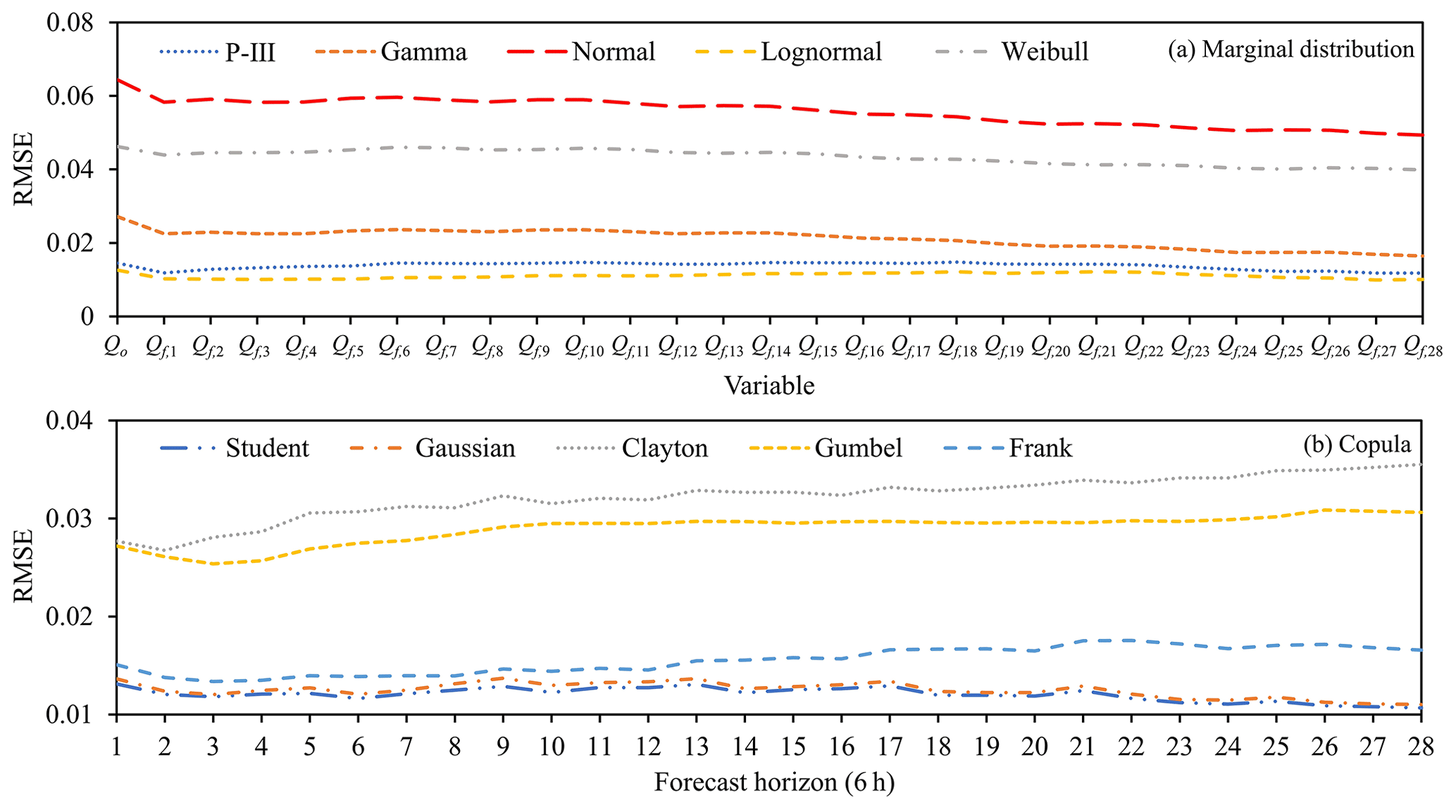
Figure 6 The RMSE values of Q_o, Q_b, and Q_f sequence marginal distributions and copula functions. 1, 2, … , 28 denote 6, 12, … , 168 h forecast horizons, respectively.

4.2.2 Sliding window length selection

Since there is no specific method or rule to calculate the sliding window length, this study adopts the CRPS metric as the objective function and the trial-and-error method to select the sliding window length. The range of window lengths is [40,200].

To facilitate the selection of the sliding window lengths, Fig. 7 shows the average CRPS values of the HUP-BMA and CHUP-BMA methods for all forecast horizons with different window lengths. It can be seen from Fig. 7 that the HUP-BMA and CHUP-BMA methods all have the lowest CRPS values at the sliding window length of 80. Therefore, 80 is the optimal window length for the ensemble forecasting study.

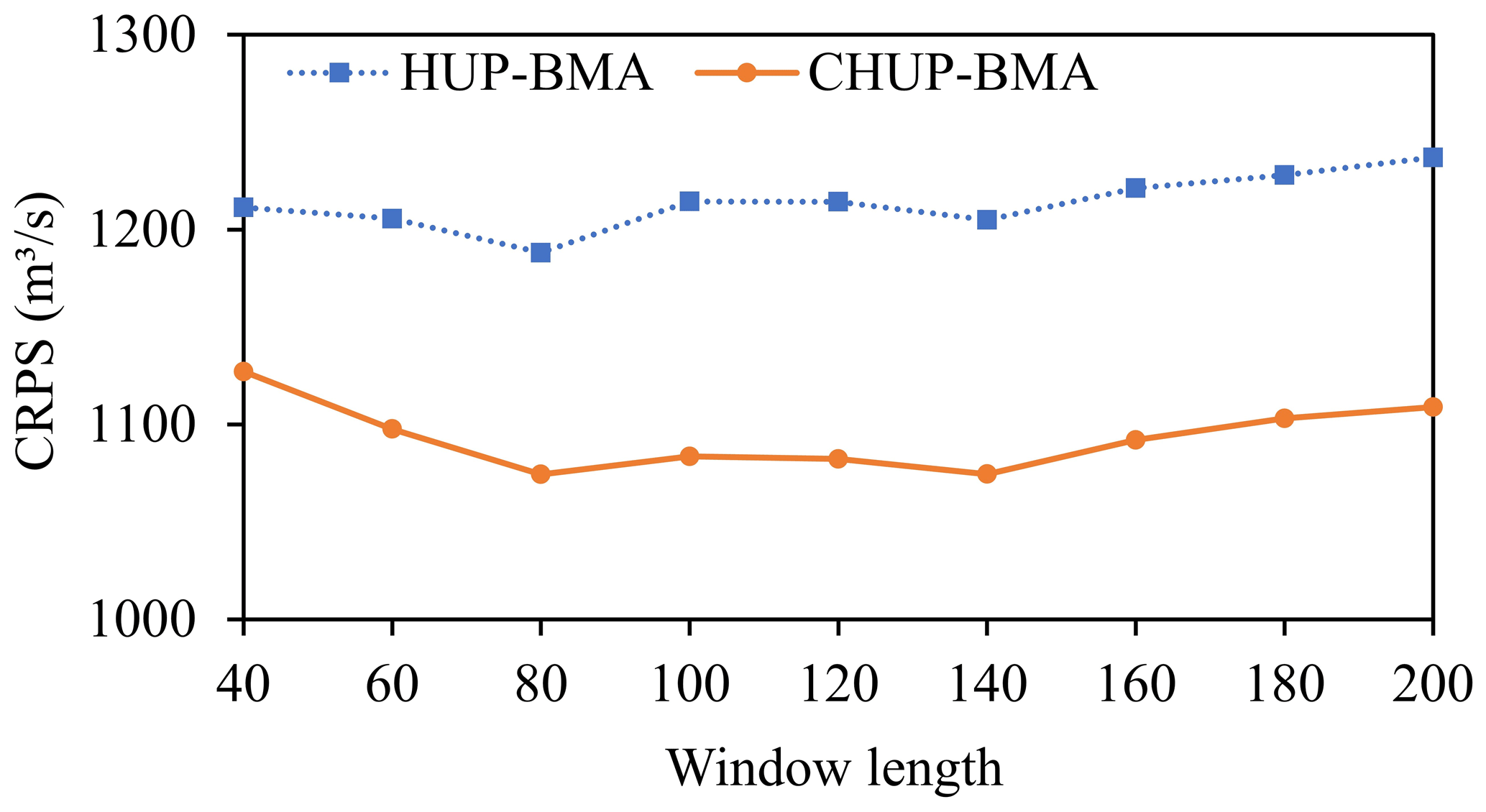
Figure 7 The average CRPS values of the CHUP-BMA and HUP-BMA methods with different window lengths.

4.2.3 Deterministic forecast results of ensemble forecast

The HUP-BMA and CHUP-BMA methods use expected values of ensemble forecasts as deterministic forecast results. In order to analyze the deterministic forecast performance of ensemble forecasts, one member with the best forecast accuracy is selected for comparative analysis based on the criteria of the relatively low RE and MAE values and relatively high NSE values, which are composed of the forecast rainfall from ECWMF, the DA-LSTM-RED model, and the objective function with mean square error to optimize the parameters.

Figure 8a–c show the NSE, MAE, and RE metrics of three deterministic forecast results, respectively. It can be seen that the NSE metrics show a decreasing trend and that the MAE metrics show an increasing trend as the forecast horizon increases, indicating a gradual decrease in forecast accuracy.

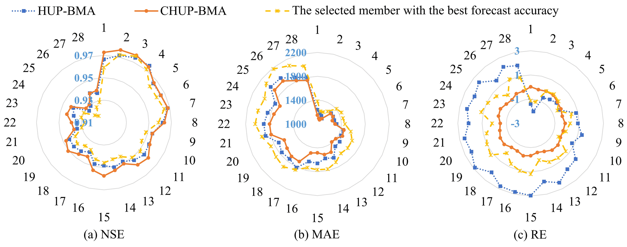
Figure 8 Deterministic forecast evaluation metrics for the HUP-BMA, the CHUP-BMA, and the selected member with the best forecast accuracy.

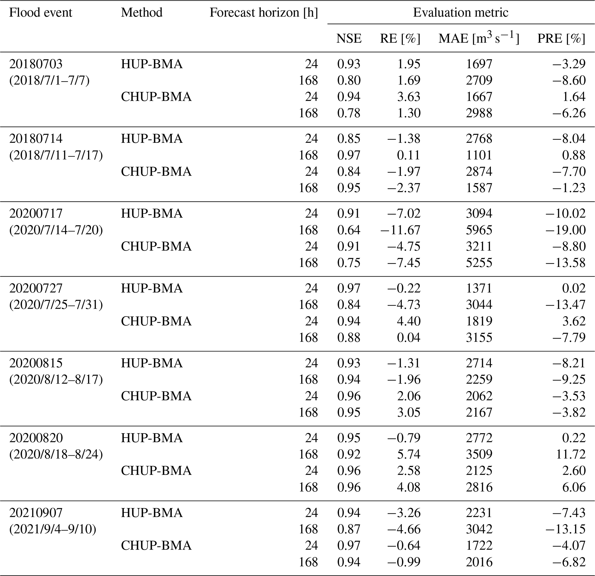
Table 4 Evaluation metrics for forecast flood events for 24 and 168 h forecast horizons.

As shown in Fig. 8a, the NSE metrics of three forecast results are at least 0.92 during the 6–168 h forecast horizons. The difference between the two is small, not more than 0.02. Among them, the CHUP-BMA method has the best NSE metrics. However, the advantage value gradually decreases as the forecast horizon increases. The NSE metrics of the HUP-BMA method are better than those of the selected forecast member in most forecast horizons. From Fig. 8b, the maximum and mean values of MAE are 1923 and 1513 m³ s⁻¹ for the CHUP-BMA method, 1999 and 1582 m³ s⁻¹ for the HUP-BMA method, and 2179 and 1719 m³ s⁻¹ for the selected forecast member, respectively. The CHUP-BMA method has the best MAE metric, with the maximum and average reduction of 10.69 % and 4.36 % relative to the HUP-BMA method, respectively. Meanwhile, the MAE values of two ensemble forecasting methods are lower than those of the selected forecast members. As shown in Fig. 8c, the maximum and mean of the RE metric are 0.02 % and −0.27 % for the CHUP-BMA method, 2.97 % and 1.36 % for the HUP-BMA method, and 1.20 % and 0.34 % for the selected forecast member, respectively. The CHUP-BMA method can reduce the RE metrics of the selected forecast member in most forecast horizons, while the HUP-BMA method has no advantage in the RE metric. Overall, ensemble forecast methods can somewhat improve the selected best member forecast accuracy. The CHUP-BMA method's expectation forecast has the best accuracy, which indicates that the copula-based CHUP-BMA method can improve the performance of the HUP-BMA method in correcting errors.

To further analyze the accuracy of ensemble forecast methods, seven floods with peaks exceeding 50 000 m³ s⁻¹ during the 24 and 168 h forecast horizons in the validation period (2017–2021) are selected for analyzing. The average relative error metric of peak (PRE) (Cui et al., 2022) is added to analyze the forecasting performance for flood peaks. Table 4 demonstrates the forecast evaluation metrics for the seven flood events. With the increase in the forecast horizon, the NSE metric shows a decreasing trend and the RE and MAE metrics show an increasing trend, indicating a gradual decrease in forecasting performance. It can be seen from Table 4 that (1) in the 24 h forecast horizon, the forecast accuracy of the two methods is similar for most flood events and quality metrics, and (2) in the 168 h forecast horizon, the forecast accuracy of the CHUP-BMA method is better than that of the HUP-BMA method in most flood events and quality metrics. The average values of NSE, RE, MAE, and PRE are 0.88, −0.63 %, 2980 m³ s⁻¹, and −4.55 % for CHUP-BMA and 0.84, −2.38 %, 3188 m³ s⁻¹, and −6.46 % for HUP-BMA, respectively, indicating an overall improvement of CHUP-BMA over HUP-BMA in forecasting accuracy.

To further demonstrate the accuracy of flood process forecasting and applicability of the two methods, four relatively large flood events are selected for comparative analysis for the 168 h forecast horizon (Fig. 9). In the 20180703 flood event (Fig. 9a), the two methods have similar forecast performance, underestimating the peak and rising water processes and overestimating the receding water process. The CHUP-BMA method has relatively low PRE and total runoff error values. The HUP-BMA method accurately forecasts the peak present time. In the 20200815 flood event (Fig. 9b), two methods underestimate the flood peak and overestimate the receding water process. The HUP-BMA method has a larger flood peak error, and the CHUP-BMA method has a better fitting performance. In the 20200820 flood event (Fig. 9c), two methods overestimate the observed flood process, with the CHUP-BMA method having the lower peak and total runoff error than the HUP-BMA method. In the 20210907 flood event (Fig. 9d), the CHUP-BMA and HUP-BMA methods underestimate the flood peak and delay the forecast peak occurring time. The former has smaller peak and water volume error.

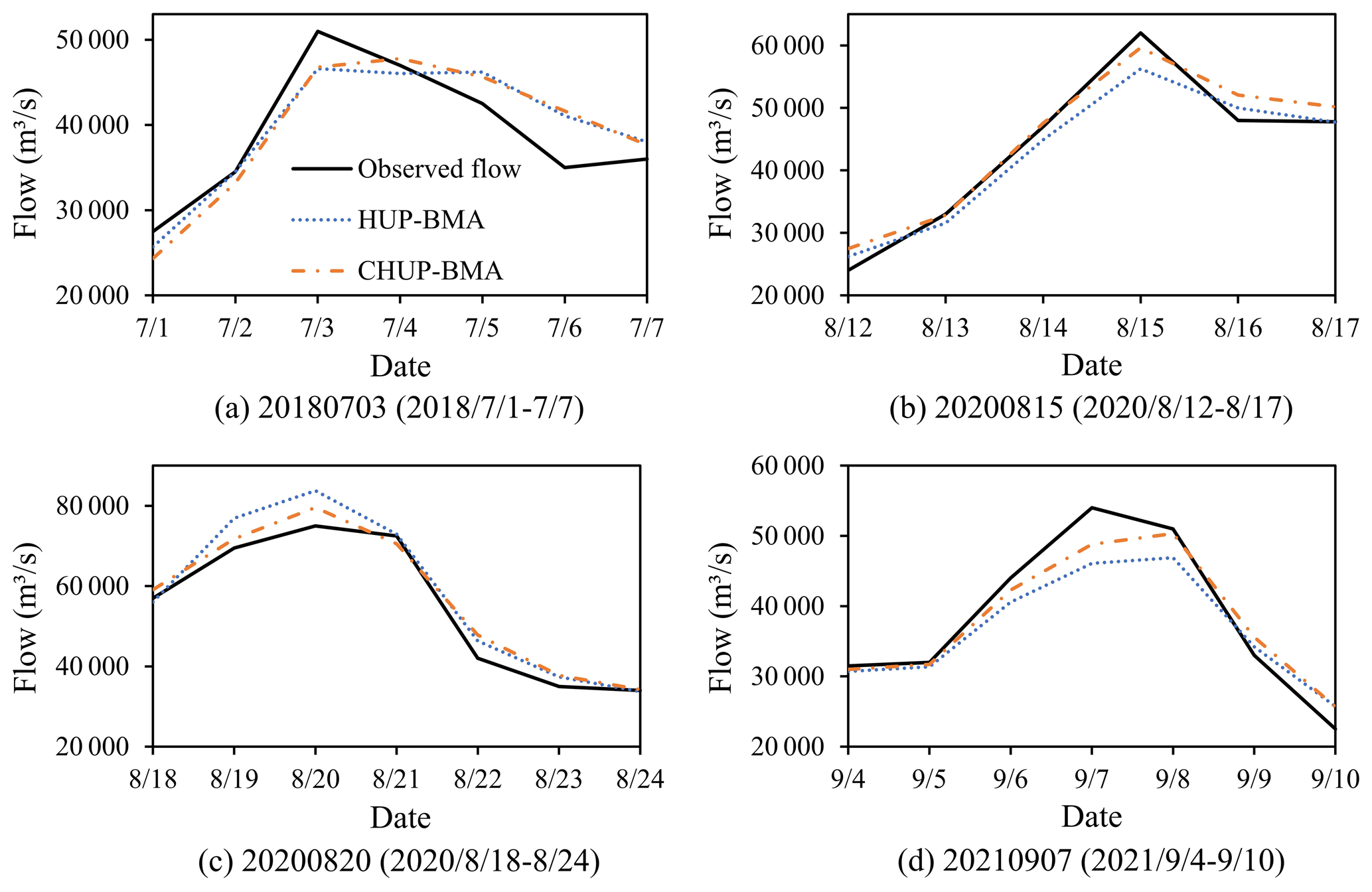
Figure 9 Forecasted flood events during the 168 h forecast horizon for the HUP-BMA and the CHUP-BMA methods.

4.2.4 Probabilistic forecast results of ensemble forecast

Evaluation of forecast interval

Figure 10a–c show the CR, IW, and PUCI metrics for the forecast interval, respectively, with a 90 % confidence level. Figure 10a shows that during the 6–168 h forecasting period, the maximum, minimum, and mean of the CR metric for the forecast interval of the CHUP-BMA method are 0.92, 0.88, and 0.89 and 0.93, 0.88, and 0.91 for the HUP-BMA method, respectively. The CR values of the two methods' forecast intervals are close to or exceed the 90 % confidence level, indicating that the forecast intervals are reliable.

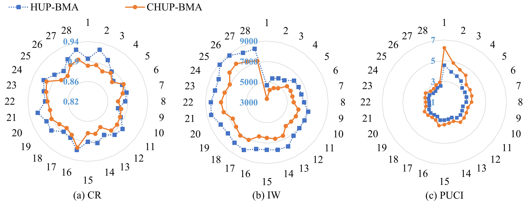
Figure 10 Evaluation metrics of forecast intervals with the 90 % confidence level of the HUP-BMA and CHUP-BMA methods.

It is obvious from Fig. 10b that the forecast interval width tends to increase with the increase in the forecast horizon, indicating that the forecast uncertainty gradually increases. The maximum, minimum, and mean of the IW metrics for the forecast interval of the CHUP-BMA method are 7820, 3337, and 6257 m³ s⁻¹ and 8888, 4662, and 7345 m³ s⁻¹ for the HUP-BMA method, respectively. The forecast intervals of the CHUP-BMA method are significantly narrower than those of the HUP-BMA method, with the maximum and average reduction of 28.42 % and 15.32 %, respectively, which indicates that the CHUP-BMA method can effectively reduce the interval width and forecast uncertainty.

From Fig. 10c, the maximum, minimum, and mean of the PUCI metric for the forecast interval of the CHUP-BMA method are 6.24, 2.65, and 3.48 and 4.55, 2.35, and 2.95 for the HUP-BMA method, respectively. The CHUP-BMA method has the higher PUCI values, indicating that the forecast interval of the CHUP-BMA method reflects the forecast uncertainty relatively well.

In summary, the CHUP-BMA outperforms the HUP-BMA method under the premise that the CR values are close to or exceed the 90 % confidence level. The CHUP-BMA method has narrower forecast intervals and better performance in quantifying forecast uncertainty. Although the HUP-BMA method has a higher CR value, its IW value is larger and the PUCI value is smaller for the long forecast horizon, indicating that the forecast interval is too conservative to reasonably estimate the uncertainty range.

In order to visually analyze the ability of the CHUP-BMA method to quantify forecast uncertainty, the forecast intervals with a 90 % confidence level of the HUP-BMA and CHUP-BMA methods for 168 h forecast horizon in the 2020 flood season are compared. It can be seen from Fig. 11 that the forecast intervals of the two ensemble forecasts can cover most of the observed flows and always cover the annual maximum flood peak, indicating that the forecast intervals are reliable. Meanwhile, the forecast intervals of the CHUP-BMA method are remarkably narrower than those of the HUP-BMA method, indicating that the forecast uncertainty of the former is relatively low, which can provide more reasonable risk information for TGR flood control decisions.

Figure 11 Forecast intervals with the 90 % confidence level for the HUP-BMA and CHUP-BMA methods from 1 July 08:00 LT to 24 September 2020 08:00 LT.

Evaluation of overall probabilistic forecast

Figure 12 shows the probability integral transform (PIT) histograms of the HUP-BMA and CHUP-BMA methods for the 24, 96, and 168 h forecast horizons. It can be significantly observed that the PIT plots of the HUP-BMA method show an upside-down-U-shaped distribution, which indicates that the forecast distribution is over-dispersed and overestimates the forecast uncertainty, explaining the phenomenon of wide intervals. Meanwhile, the PIT plot of CHUP-BMA is more uniformly distributed than that of the HUP-BMA method, which can obtain a better calibration performance.

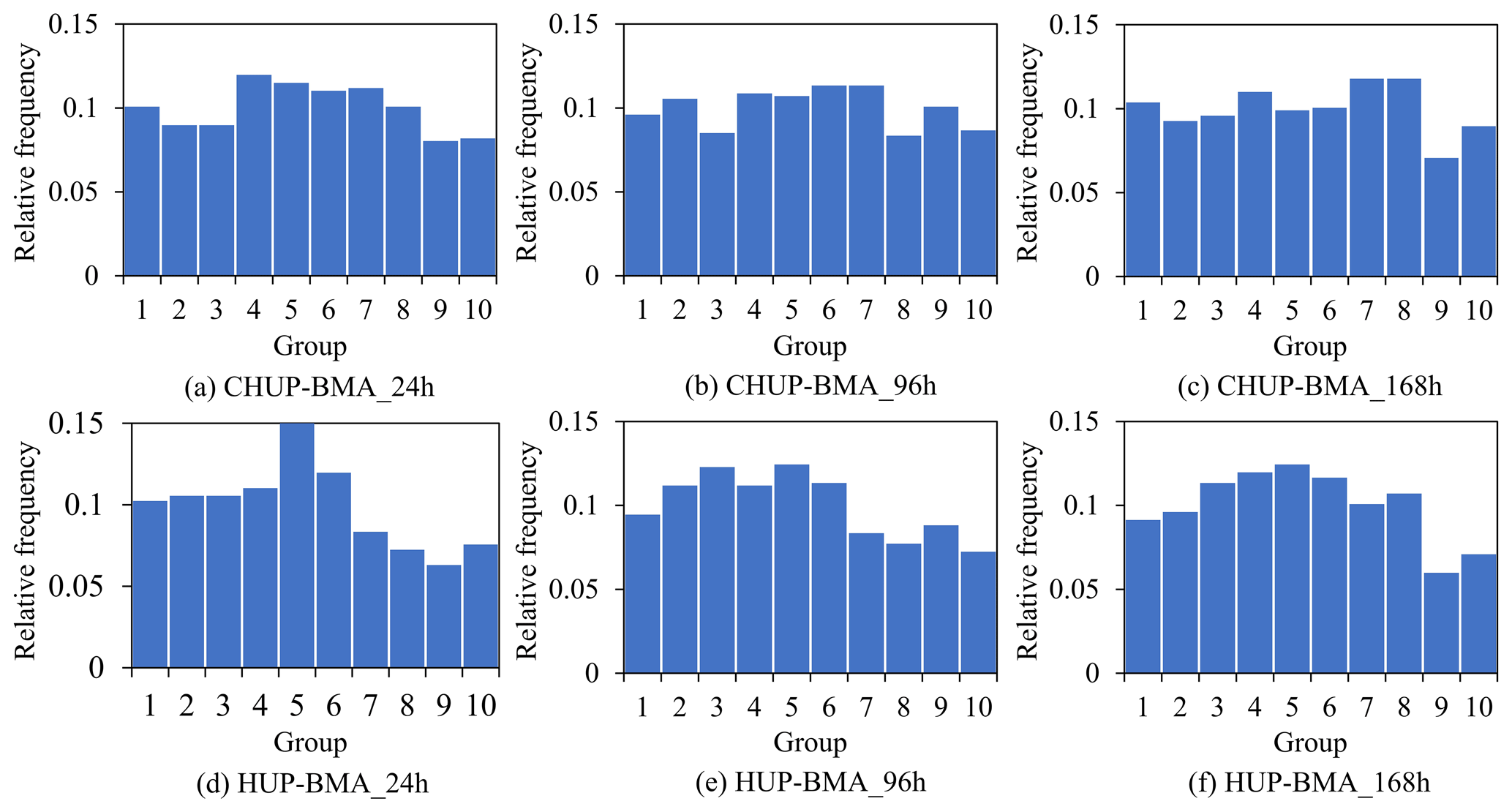
Figure 12 The probability integral transform (PIT) histograms of the HUP-BMA and CHUP-BMA methods for the ensemble forecasts of the 24, 96, and 168 h forecast horizons.

Meanwhile, Fig. 13a–c show the evaluation metrics of α_index, IGS, and CRPS metrics for the two ensemble probabilistic forecasts, respectively. It can be seen from Fig. 13a that the α_index metrics of the CHUP-BMA method-based probabilistic forecasts are significantly higher than those of the HUP-BMA method in the 6–168 h forecast horizons. Among them, the maximum, minimum, and mean of the α_index metric for CHUP-BMA method-based probabilistic forecasts are 0.98, 0.93, and 0.97 and 0.95, 0.88, and 0.93 for the HUP-BMA method, respectively. The α_index metric of the CHUP-BMA method-based probabilistic forecast is closer to the perfect value of 1, indicating that its probability forecast is the more reliable one.

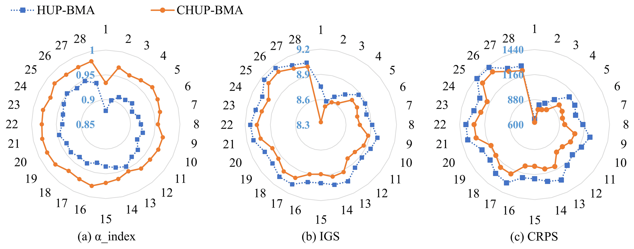
Figure 13 Evaluation metrics of α_index, IGS, and CRPS metrics of two ensemble forecasts. The α_index metric can assess the reliability of ensemble forecasts, while the IGS and CRPS metrics can reflect the reliability and sharpness of the ensemble forecast. The closer the α_index metric is to 1 and the smaller the IGS and CRPS metrics are, the better the performance of the ensemble forecast.

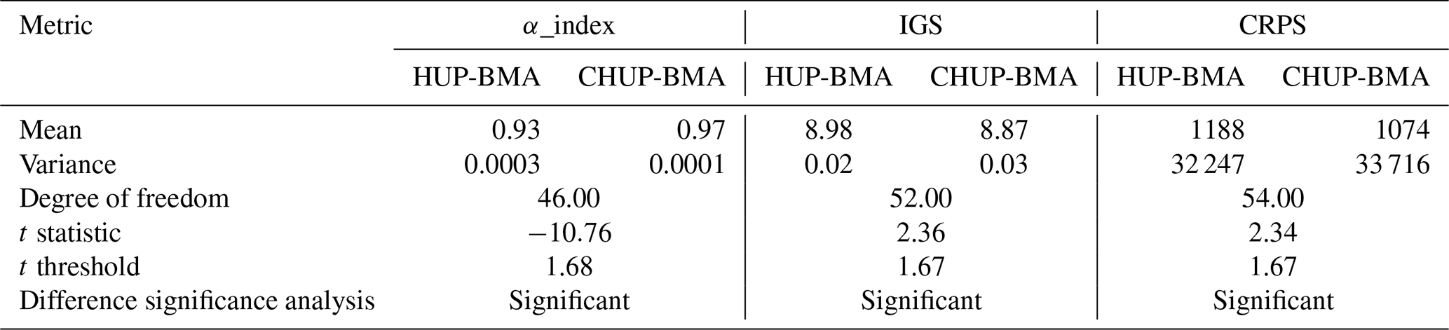
Table 5 T test results of ensemble forecast metrics at the 0.05 significance level.

It can be seen from Fig. 13b that the IGS values of the two methods gradually increase with the increase in the forecast horizon, indicating that the forecast uncertainty gradually increases. The maximum, minimum, and mean of the IGS metric for the CHUP-BMA method are 9.10, 8.33, and 8.87 and 9.16, 8.59, and 8.98 for the HUP-BMA method, respectively. It can be seen that the IGS metrics of the CHUP-BMA method are consistently lower than those of the HUP-BMA method, which indicates that the CHUP-BMA method has better ensemble forecast performance relative to the HUP-BMA method by assigning a higher probability density around the actual values.

As shown in Fig. 13c, the CRPS values of the two methods are lower than the MAE values of the selected member (Fig. 8b), indicating that the probabilistic forecasts are effective and can fit the probabilistic distribution of the target values well. Meanwhile, during the 6–168 h forecast horizons, the maximum, minimum, and mean of the CRPS metric for the CHUP-BMA method are 1356, 625, and 1074 m³ s⁻¹ and 1425, 662, and 1188 m³ s⁻¹ for the HUP-BMA method, respectively. It can be seen that the CRPS values of the CHUP-BMA method are lower than those of the HUP-BMA method, with a maximum and average reduction of 17.86 % and 9.71 %, respectively. It can be seen that the CHUP-BMA method can fit the posterior distribution of the actual values better and effectively improve the probabilistic forecast performance of the HUP-BMA method.

From Table 5, it can be seen that the t statistic values at the 0.05 significance level for all three metrics are higher than the threshold value, indicating that there is a significant difference between the scores of the CHUP-BMA and HUP-BMA methods; i.e., the CHUP-BMA method is significantly better than the HUP-BMA method for ensemble forecasting metrics and performance.

In summary, the CHUP-BMA method considers the influence of the initial state on the ensemble forecast, bypasses the normal quantile transformation of the HUP-BMA method, derives the posterior distribution of the target flow without restrictions, and improves the probabilistic forecast performance of the HUP-BMA method. Therefore, the ensemble forecasting by CHUP-BMA method can provide more reasonable and reliable risk information for the TGR.

5 Conclusion and prospects

In this study, we propose a novel CHUP-BMA method, which can not only consider the influence of the initial state on the ensemble forecast, but also avoid the assumption of normal distribution in the HUP-BMA method and derive the posterior distribution function more accurately. An ensemble forecast scheme that consists of two forecasted precipitation, two hydrological models, and two objective functions of parameter calibration was established. The ensemble forecasting performance of the HUP-BMA and CHUP-BMA methods was discussed from the perspective of deterministic and probabilistic forecasts. The flood ensemble forecasting experiment with 6–168 h forecast horizons was conducted in the Xiangjiaba–TGR dam site interval basin. The main conclusions were summarized as follows:

1. The two ensemble forecasting methods can improve the members' forecast accuracy. The proposed CHUP-BMA method performs better than the HUP-BMA method, and the MAE metric is reduced by a maximum of 10.69 % within 6–168 h forecast horizons.

2. The coverage rate of the forecast interval of the CHUP-BMA method is close to or exceeds the specified 90 % confidence level, and the forecast interval is significantly narrower than that of the HUP-BMA method, with a maximum reduction of 28.42 % during 6–168 h forecast horizons, which can effectively reduce the forecast uncertainty.

3. The probabilistic forecast of the CHUP-BMA method has better reliability and sharpness, and its CRPS values are reduced by a maximum of 17.86 % relative to the HUP-BMA method, which indicates that the CHUP-BMA method can fit the posterior distribution of the actual values better.

4. The CHUP-BMA method can derive the posterior distribution of the target flow without restriction under the condition that the initial constraint is considered, which brings the BMA method closer to perfection. Therefore, it is more suitable for flood forecasting in the 6–168 h forecast horizons and provides reliable risk information for reservoir scheduling decision-making.

The present study focuses on flood ensemble forecasting for the TGR 6–168 h forecast horizons. Future studies can explore the ensemble forecasting performance of the proposed CHUP-BMA method for longer forecast horizons and further validate the effectiveness of the proposed method in global basins. Meanwhile, the vine copula, which facilitates multivariate joint distribution modeling, can be considered for constructing the CHUP-BMA method and exploring its advantages and effectiveness in ensemble flood forecasting. The effective way or method of guiding reservoir scheduling based on ensemble forecasts can also be further explored so that ensemble forecasts can be widely used in decision-making.

Appendix A: The model parameters for ensemble membership

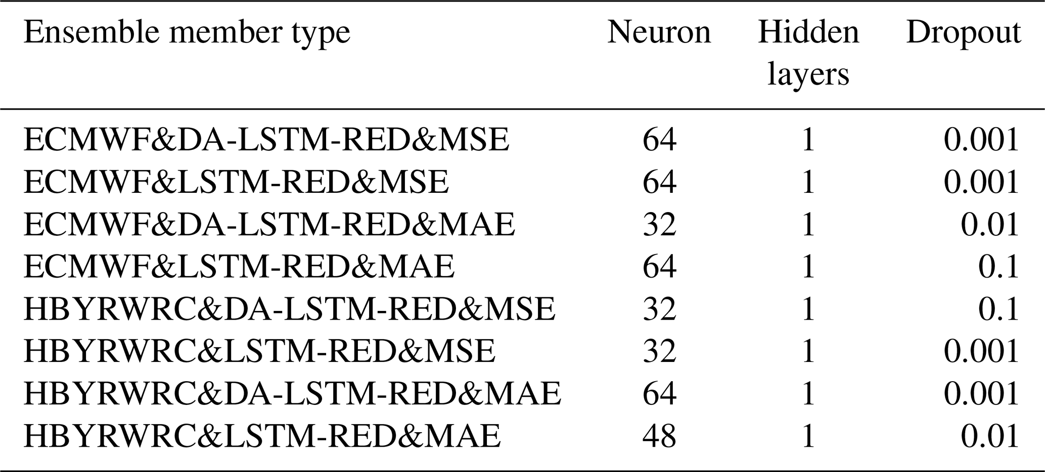
We set the number of neural network layers and neurons to be the same for the encoding and decoding processes, with trial-and-error preferences for the number of hidden layers, neurons, and dropout. Meanwhile, the batch size, epoch, and learning rate are set to 100, 500, and 0.001, respectively. The different model parameters are shown in Table A1.

Table A1 The model parameters for ensemble membership.