Enhancing long short-term memory (LSTM)-based streamflow prediction with a spatially distributed approach

Deep learning (DL) algorithms have previously demonstrated their effectiveness in streamflow prediction. However, in hydrological time series modelling, the performance of existing DL methods is often bound by limited spatial information, as these data-driven models are typically trained with lumped (spatially aggregated) input data. In this study, we propose a hybrid approach, namely the Spatially Recursive (SR) model, that integrates a lumped long short-term memory (LSTM) network seamlessly with a physics-based hydrological routing simulation for enhanced streamflow prediction. The lumped LSTM was trained on the basin-averaged meteorological and hydrological variables derived from 141 gauged basins located in the Great Lakes region of North America. The SR model involves applying the trained LSTM at the subbasin scale for local streamflow predictions which are then translated to the basin outlet by the hydrological routing model. We evaluated the efficacy of the SR model with respect to predicting streamflow at 224 gauged stations across the Great Lakes region and compared its performance to that of the standalone lumped LSTM model. The results indicate that the SR model achieved performance levels on par with the lumped LSTM in basins used for training the LSTM. Additionally, the SR model was able to predict streamflow more accurately on large basins (e.g., drainage area greater than 2000 km²), underscoring the substantial information loss associated with basin-wise feature aggregation. Furthermore, the SR model outperformed the lumped LSTM when applied to basins that were not part of the LSTM training (i.e., pseudo-ungauged basins). The implication of this study is that the lumped LSTM predictions, especially in large basins and ungauged basins, can be reliably improved by considering spatial heterogeneity at finer resolution via the SR model.

1 Introduction

Reliable streamflow prediction is critical in water resources management. Following recent developments in artificial intelligence (AI), an increasing number of hydrological studies have focused on adopting deep learning (DL) techniques, such as long short-term memory (LSTM), to improve basin-scale streamflow prediction compared with traditional physically based hydrological models and conventional machine learning (ML) algorithms (Kratzert et al., 2018; Frame et al., 2021; Gauch et al., 2021). LSTM is a type of recurrent neural network (RNN) that can capture long-term dependencies in hydrological time series data and has demonstrated promising results in tasks such as streamflow prediction (Kratzert et al., 2018; Gauch et al., 2021), precipitation forecasting (Tao et al., 2021), and drought monitoring (Wu et al., 2022). A recent large-sample model intercomparison study, namely the Great Lakes Runoff Intercomparison Project in the Great Lakes region (GRIP-GL; Mai et al., 2022a), showed that a LSTM model exhibited significant superiority in streamflow predictions compared with 12 other physically based hydrological models, regardless of whether they were lumped or spatially distributed (Mai et al., 2022a). The development of LSTM in hydrology has been driven by the need for more accurate and sophisticated models that can handle the complex and non-linear relationships in hydrological processes.

Despite the recent popularity of data-driven modelling (e.g., ML and DL models) in hydrological modelling studies, process-based hydrological models (physically based or conceptual models) continue to be used for operational streamflow forecasting. In contrast with data-driven prediction, traditional process-based models often rely more on a spatially distributed representation of the region or basin being simulated. They utilize gridded meteorological forcings and, more importantly, break the basin up into various smaller response units, such as grid cells (fully distributed model) or subbasins (semi-distributed model). Compared with lumped models, distributed models consider spatial variability at a finer resolution and also incorporate the routing process within the simulated basin. With the recognition that data-driven models and process-based models possess distinct advantages, the hybridization of these two types of models has drawn growing attention in environmental modelling studies. Hybrid models can be categorized into two primary structural types: serial and parallel. In most cases, a serial hybrid model involves the sequential coupling of one data-driven model and one process-based model (Hunt et al., 2022). This is typically achieved by feeding (to train) a data-driven model with the outputs of a process-based model (Frame et al., 2021; Liu et al., 2021; Nevo et al., 2022), which implies that the data-driven model usually serves as a post-processor within a hybrid modelling workflow. On the contrary, a recent study by Bindas et al. (2024) employed a DL network to infer the parameterizations of a river routing model for enhanced streamflow prediction. In a parallel hybrid model, the data-driven model and process-based model are integrated in parallel with each simulating different processes (Slater et al., 2023). In general, these hybrid modelling approaches allow researchers, to a certain extent, to incorporate spatial variability in input variables into the data-driven prediction scheme.

It is widely acknowledged that having ample training data is advantageous for DL models. Kratzert et al. (2018) argued that training a local LSTM streamflow model at an individual gauged basin is an inferior approach compared with training a regional LSTM model over many gauged basins. They trained a single LSTM model for lumped rainfall–runoff simulation on a large sample of 241 basins using meteorological forcing data and static basin attributes and then compared the performance of this regionally trained LSTM streamflow model to that of individual local LSTM streamflow models trained separately for each of the 241 basins. The results revealed that the regionally trained LSTM model was able to outperform the local LSTM models. Nevertheless, in previous studies regarding LSTM-based streamflow prediction (to the best of our knowledge), most regionally trained LSTM models only consider the spatial heterogeneity between training basins where LSTM inputs are at the lumped training basin scale. That is, each attribute (i.e., LSTM input variable) is computed for the entire basin and the basin is considered a single response unit such that streamflow is only predicted at the outlet of the basin (Kratzert et al., 2018, 2019; Feng et al., 2020; Gauch et al., 2021; Xie et al., 2022; Arsenault et al., 2023; Tang et al., 2023; Pokharel et al., 2023). Typically, this involves cropping the gridded dynamic input variables (e.g., precipitation and temperature) to the basin polygon and calculating a basin average (or weighted average) to produce the lumped time series of the dynamic input variables (Lees et al., 2022).

The rationale behind employing a lumped model is the architectural limitation of LSTM networks: they are not compatible with gridded data (i.e., image-like data) with various shapes (i.e., basin outlines) as inputs. Additionally, a lumped model enables effective learning of static basin attributes, such as drainage area and frequency of high precipitation (Kratzert et al., 2019). However, the aggregation of climatic forcings results in neglecting the heterogeneous spatial distribution of various rainfall events. A study by Hunt et al. (2022) explained that a lumped LSTM probably failed to appropriately characterize rainfall over a large and arid basin due to averaging rainfall to the basin scale. Wang and Karimi (2022) argued that lumped LSTM rainfall–runoff models are unable to fully utilize the spatial variability in input features. In their experiments, the spatial variability in rainfall was represented by a 20-element vector feature. For each of the 10 basins where they trained the LSTM, the vector consists of rainfall data at all hydrological response units within the basin. Their results show that LSTM models trained on spatially distributed rainfall data outperformed those driven by basin-averaged rainfall data. Nonetheless, their method does not clarify how to generalize the process of supplying the LSTM model with spatially distributed rainfall information in the context of predicting outcomes in ungauged basins (PUB).

Conceptually, the predictive accuracy of lumped hydrological modelling will eventually degrade as basin size increases. This is due to the fact that meteorological forcing inputs are simply not well approximated by assuming they are constant over space. For example, in their paper presenting the CAMELS (Catchment Attributes and Meteorology for Large-sample Studies) dataset of attributes for 671 basins in the contiguous United States, Addor et al. (2017) cautioned against using the largest of these basins for lumped hydrological modelling. They argued that the significance of basin-averaged input attributes diminishes with an increase in basin drainage area, because a larger basin tends to necessitate a heightened consideration of spatial heterogeneity, requiring the incorporation of a spatially distributed representation. Nevertheless, the threshold at which basin area leads to poor lumped model performance is not precisely known and will likely vary by watershed location. In a study of benchmarking multiple hydrological models, Newman et al. (2017) excluded basins in the CAMELS dataset over 2000 km² in drainage area. Additionally, a lumped LSTM modelling study by Kratzert et al. (2019) and the original set of basins in the Caravan lumped global large-sample hydrology dataset (Kratzert et al., 2023) both employ 2000 km² as an upper threshold. Given the past use of the 2000 km² threshold, we apply this criterion to define a “large basin” in our study.

Hydrological routing across a drainage network is a general technique commonly used in distributed hydrological models, and it allows the model to represent the transport of water more accurately throughout large, heterogeneous basins. A recent study by Bindas et al. (2024) presented a novel differentiable river routing method to improve the streamflow prediction in a single large basin. They employed a regionally trained LSTM to predict discharge at the subbasin-level and then map the LSTM predictions to a river network for routing. The results of the final routing model showed promise by simulating predicted subbasin-level discharge from a lumped LSTM. However, their study presented limited empirical evidence demonstrating the superiority of their routing model over the lumped LSTM. Specifically, the comparison was conducted within one single basin for a short testing period of 1 year, and the routing model outperformed the lumped LSTM in one of the three untrained gauges with more than 2000 km² of drainage area. As for methodology, an intermediate (scale-specific and basin-specific) process is required to translate the LSTM predictions into lateral flow inputs for each reach in the river network. Furthermore, the routing model requires the training of a multilayer perceptron network to update the parameters. As such, their basin-scale approach is challenging to directly generalize to new basins or to different spatial scales for modelling.

Our study aims to identify an easy-to-implement, generalizable, regional-scale (or larger) approach for applying spatially distributed inputs to effectively improve upon lumped data-driven streamflow prediction, especially in large, ungauged basins. In pursuit of this goal, we propose the Spatially Recursive (SR) model. The SR model first employs a lumped data-driven prediction model (regionally trained on a large sample of basins) to predict local streamflow at subbasins discretized from the basin of interest. Then, it utilizes a semi-distributed hydrological routing-only model, capable of explicit lake simulation, to route subbasin streamflow to the basin outlet. The data-driven prediction model is considered spatially recursive because it is trained at the basin scale and further applied at the subbasin scale to incorporate finer-resolution forcing data and subbasin attributes.

The paper is structured as follows: Sect. 2 provides a description of the SR model, datasets, and experimental design; Sect. 3 presents key results and discussion; and, finally, Sect. 4 concludes the findings and outlines future work.

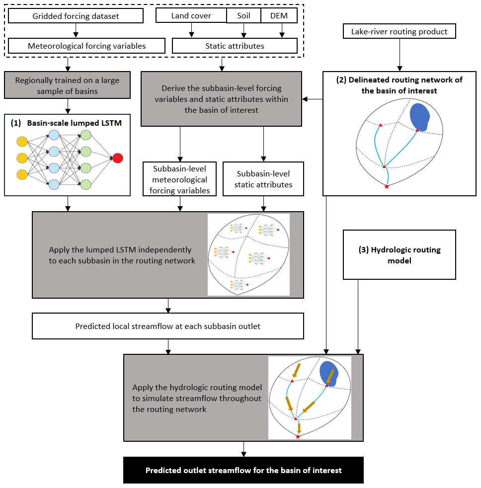
Figure 1 The Spatially Recursive model workflow for an arbitrary basin of interest. Note that the workflow is conceptually model-agnostic (e.g., the lumped LSTM can be replaced by another data-driven model), while each component needs to generate outputs compatible with other components. Components with multiple arrows are utilized multiple times throughout the workflow.

2 Material and methods

2.1 Overview of the Spatially Recursive (SR) model

The proposed SR model is composed of three workflow components (see Fig. 1): a regional LSTM for basin outlet streamflow prediction that is trained using a large sample of basins, a vector-based lake–river routing network that breaks up basins into subbasins, and a process-based routing model that only simulates the movement of LSTM-predicted subbasin-level streamflow through the routing network. The fundamental concept of the SR model is to firstly employ a regional LSTM to predict local streamflow at each subbasin outlet (delineated in the lake–river routing network) for a basin where streamflow at the basin outlet is of interest. Note that local streamflow for a subbasin is defined as the streamflow at the subbasin outlet that would occur if there were no upstream subbasins. Then, the predicted streamflow at each subbasin outlet serves as input to the routing-only model, which simulates how water is transported through the lake–river routing network and, ultimately, the streamflow at the basin outlet.

In general, none of the three workflow components are novel when considered individually, as numerous existing studies have explored and assembled them in various ways. The distinctive aspect of our research lies in the smooth coupling of the LSTM and the routing model. The regionally trained LSTM is applied to directly produce the local streamflow at the subbasin scale (i.e., the spatial scale of the routing model); thus; there is no need for scale transformation when we use the LSTM prediction as the direct input to the routing model. Additionally, the SR model does not require any further training/calibration of either the regional LSTM or the routing model, making it generalizable to any designated gauge or basin outlet within the LSTM training region. The lake–river routing product, such as the MERIT Hydro global database (Yamazaki et al., 2019) and the North American Lake–River Routing Product (NALRP; Han et al., 2020), which features vector-based watershed discretization, should typically have a finer spatial resolution to break up each basin polygon into subbasins, at least for the majority of the streamflow gauging stations used for LSTM training. The following subsections explain the specifics of the components that we selected in this study to demonstrate the spatially recursive modelling approach.

2.1.1 GRIP-GL lumped LSTM

In this study, we precisely replicated the lumped LSTM built for streamflow prediction in the Great Lakes region of North America by Mai et al. (2022a). That is, we trained our version of the lumped LSTM model using the same hyperparameters and input features as the LSTM model trained in the GRIP-GL project. The decision to employ an existing lumped LSTM for streamflow prediction, rather than attempting to add more basins and retrain a new LSTM, was intentional, as we wanted to explicitly demonstrate that the proposed spatially distributed methodology works to improve upon an existing lumped LSTM without the need for LSTM retraining.

A brief summary of the model setup, training, and testing procedures of the lumped LSTM is presented here. Section S3 in the Supplement details the hyperparameter settings and the full list of all model input features. Following the training procedures outlined by Mai et al. (2022a), our trained model is an ensemble of 10 LSTM models with the same architecture but different random seeds, and the final prediction is the average of the 10 models' outputs. Each LSTM model was simultaneously trained on 141 gauged basins (also referred to as “calibration basins” in the GRIP-GL project) located in the Great Lakes region, over the period from January 2000 to December 2010 (referred to as the “calibration period” in GRIP-GL). The LSTM model was constructed using the NeuralHydrology Python library (Kratzert et al., 2022). It was implemented to conduct sequence-to-one prediction – that is, the LSTM model predicts the average streamflow for a single day based on the input sequence of the previous 365 d of data.

The input features were derived for each basin, which include the target variable (observational streamflow at the daily timescale), 9 dynamic variables (meteorologic forcings; listed in Table S2 in the Supplement), and 30 static basin attributes describing soils, topography, land cover types, and climate. The observed discharge data are from either Water Survey Canada (WSC) or the United States Geological Survey (USGS). The meteorologic forcings and climatic attributes were taken from the Canadian Surface Reanalysis Version 2 (CaSR-v2; previously known as the Regional Deterministic Reanalysis System, or “RDRS” for short; Gasset et al., 2021). CaSR-v2 is a gridded reanalysis product that covers North America with a 10 km × 10 km spatial resolution on an hourly time step; this product was downloaded for the region from the Canadian Surface Prediction Archive (CaSPAr; Mai et al., 2020). Soil attributes were derived from the Global Soil Dataset for Earth System Models (GSDE; Shangguan et al., 2014). Topological attributes (e.g., mean elevation, mean slope) were computed from the HydroSHEDS digital elevation model (DEM) product (Lehner et al., 2008). The North American Land Change Monitoring System (NALCMS) product was used to derive the land cover attributes. The target variable and dynamic variables were aggregated from an hourly to a daily timescale. All dynamic variables and static attributes were spatially averaged for each gauged basin in the study. All input features derived for our replication of the GRIP-GL LSTM model were completely consistent with the derived input features in the original GRIP-GL study. This consistency check against GRIP-GL was important because our LSTM input derivation scripts are reapplied here for numerous and generic smaller subbasin polygons. Most importantly, the resultant trained GRIP-GL LSTM model rebuilt here generated practically identical quality hydrographs to the GRIP-GL LSTM in Mai et al. (2022a), with differences in the median Kling–Gupta efficiency (KGE) performance metric of less than 0.01 (due only to different random seeds used in training).

After the model training, the lumped LSTM model was evaluated in three validation experiments according to the testing procedures outlined by Mai et al. (2022a). These three validation experiments are used consistently throughout this study and are listed as follows:

1. temporal validation – conducted for 141 calibration basins that were used to train the LSTM, predicting the daily streamflow over the period from January 2011 to December 2017 (referred as the “validation period” in GRIP-GL);

2. spatial validation – conducted for 71 basins that were not used for model training (referred as the “validation basins” in GRIP-GL), predicting the daily streamflow over the training/calibration period (January 2000 to December 2010);

3. spatiotemporal validation – conducted for the 71 validation basins, predicting the daily streamflow over the validation period (January 2011 to December 2017).

Note that we used the term “validation” and “testing” interchangeably in this study in order to be consistent with the experimental design of GRIP-GL; it is not same as the “validation” terminology normally used in machine learning applications.

2.1.2 Spatially distributed prediction based on a lake–river routing network

The lake–river routing network for an arbitrary basin defines the connectivity between the lakes/reservoirs (river channels and subbasins) as well as initial values for subbasin, lake, and channel characteristics required for running a spatially distributed hydrological simulation. A routing product is defined as a collection of routing networks covering large geographic regions, and all included networks in a routing product should be delineated using the same source geographic information system (GIS) products (e.g., Lake polygons and DEM) (Han et al., 2023).

In this study, we tested our SR model with two routing products: the GRIP-GL common routing product (used in Mai et al., 2022a) and the North American Lake–River Routing Product v2.1 (NALRP; Han et al., 2020). Both products were generated by the BasinMaker Python library (Han et al., 2023), which supports the delineation of vector-based routing networks from any DEM and user-defined lake polygons. The GRIP-GL common routing product was derived from the HydroSHEDS DEM, with a spatial resolution of 3 arcsec. The river network and subbasin (discretization) were defined by a constant flow accumulation threshold of 5000; that is, for a given point of interest, the contributing drainage area would be at least 5000 DEM cells, which corresponds to approximately 40.5 km². On the other hand, the NALRP was produced based on the MERIT DEM (Yamazaki et al., 2019) with the same 3 arcsec resolution, and the value of flow accumulation threshold is 2000 DEM cells (approximately 16.2 km²). Additionally, attributes of lakes were taken from the HydroLAKES database (Messager et al., 2016) for both the GRIP-GL routing product and the NALRP. While the NALRP product included all lakes in HydroLAKES, the GRIP-GL routing product does not include small lakes with an area of less than 5 km².

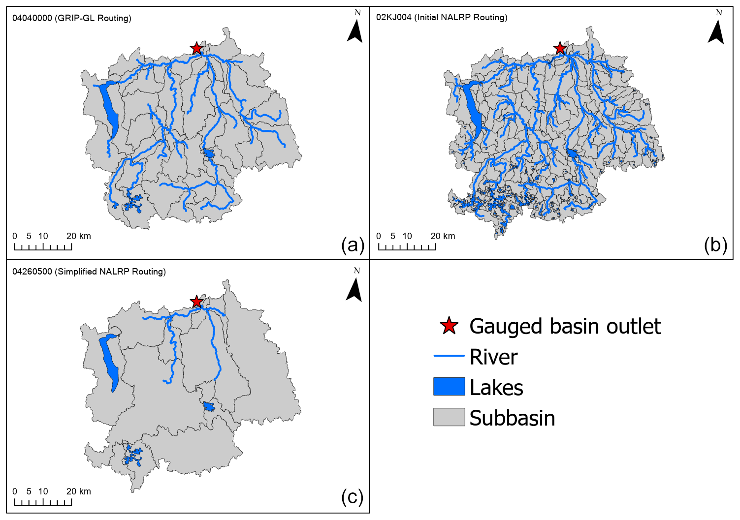
Figure 2 An example lake–river routing network for the Ontonagon River watershed (USGS gauge ID: 04040000), which is one of the GRIP-GL calibration basins: (a) the network from the default GRIP-GL common routing product; (b) the network from the initial NALRP without simplification; (c) the simplified NALRP network delineated by a minimum lake area of 5 km² and a minimum subbasin drainage area of 500 km².

We use the GRIP-GL routing product directly in order to replicate in our SR model the precise routing networks that Mai et al. (2022a) used for their semi-distributed hydrological models. The average subbasin size in the routing networks of all GRIP-GL basins is approximately 131 km². In contrast, we used the NALRP product here to provide flexibility to run our SR model in Non-GRIP-GL basins and to evaluate SR model sensitivity to alternative routing model configuration decisions. The BasinMaker library includes post-processing functions to further simplify the routing networks in the NALRP. When applying simplification to the routing network, the resolution of the routing network was reduced (Han et al., 2023) by incorporating fewer vector elements (e.g., river channels and subbasin polygons) into the routing network. For example, users can specify a minimum lake area threshold, to remove the lakes with an area smaller than the threshold, and a minimum subbasin drainage area (MDA) threshold, to merge upstream subbasins (with a drainage area smaller than the MDA threshold) to their downstream subbasin. It should be noted that the subbasin will not be merged if there is a lake or gauge located within it. Figure 2 shows a single basin discretized into three example lake–river routing networks, including the GRIP-GL routing network in Fig. 2a, the original high-resolution NALRP network in Fig. 2b, and a simplified NALRP network in Fig. 2c (derived from the original NALRP network by applying BasinMaker functions). Note that our lake subbasins include only one lake that is completely contained within the subbasin boundary and our non-lake subbasins only have a single channel reach.

As shown in Fig. 1, given the trained LSTM and the corresponding lake–river routing network discretizing a basin into subbasins, LSTM input features at the subbasin level need to be derived. This derivation is based on the original geospatial data and spatiotemporal data (see Sect. 2.1.1) and, thus, leverages the inherent spatial variability in the original data (as opposed to simply applying the basin-scale average input features in a basin to all the subbasins in that basin). With subbasin-level LSTM input features, the lumped LSTM is then deployed in each subbasin to predict the local subbasin outlet streamflow.

2.1.3 Routing-only mode in the Raven hydrological modelling framework

In this study, we constructed a physically based routing-only model in the Raven hydrological modelling framework (Craig et al., 2020) to move local subbasin outlet streamflow through the routing network in each basin. Note that the lake–river routing network generated by BasinMaker incorporates all of the necessary Raven routing model inputs and parameters (e.g., channel roughness and lake outlet characterization).

The intermediate results from our previous step in Sect. 2.1.2 (i.e., the LSTM local streamflow predictions at the subbasin level) can be seen as distributed subbasin-specific streamflow fluxes at various points within a routing network of streams and lakes (if there are any). The routing-only mode in the Raven framework can simulate the routing of distributed surface runoff (Han et al., 2020; Craig et al., 2020), but here we use it for the first time to route local subbasin outlet streamflow. This is accomplished within Raven by representing the local streamflow input (at each subbasin) as hourly precipitation instantly flushing to the subbasin outlet.

The routing model combines this local streamflow at an hourly time step with the upstream subbasin streamflow that was routed from the subbasin inlet to the subbasin outlet. This process continues from upstream to downstream subbasins to the basin outlet. The routing model time step is hourly, even though input streamflow from the LSTM comprises daily averages. We transformed the daily LSTM streamflow predictions to hourly routing simulation inputs by assuming that the streamflow is constant over the day. That is, for a given date, the LSTM-predicted streamflow is assigned to all 24 hourly time steps. The simulated hourly streamflow at each basin outlet (stream gauge) is aggregated to daily streamflow, which is the final prediction of the SR model.

The routing model is initialized with the lakes filled to the crest outlet elevation (point of zero outflow). For lake subbasins, the flushing operation sends all local subbasin streamflow into the lake instantly (rather than the subbasin outlet at the outlet of the lake), and it then becomes subject to the lake routing process in Raven. As water area is an input attribute in our LSTM, the LSTM has implicitly been trained to at least partially reflect lake routing impacts. Hence, our approach within Raven means that, for lake subbasins, the local subbasin streamflow delivery to the subbasin outlet is only approximate, as this typically small fraction of the total streamflow reaching the subbasin outlet has lake routing impacts applied in two ways instead of only one. This approximation is unavoidable within the Raven modelling system; however, to be clear, the impacts are negligible given that, for most lakes, local subbasin streamflow is only a small fraction of the total streamflow entering the lake considering all upstream subbasins.

The Raven framework provides the option to manipulate the routing algorithms and to calibrate routing-related parameters. In this study, we utilized the default configurations of the Raven framework and refrained from calibrating the routing-only model. We selected the diffusive wave channel routing option (where an analytical solution to the diffusive wave equation is used to relate inflow and outflow in each reach), and level-pool outflows from lakes are assumed to be governed by the broad-crested weir equation. As subbasin-level streamflow is predicted by a calibrated (trained) lumped LSTM model, we assume that routing calibrated fluxes through a reasonably configured default routing model will typically yield reasonable quality results. Effectively, this approach provides a lower-bound estimate of the SR model performance given that the routing model parameters are uncalibrated.

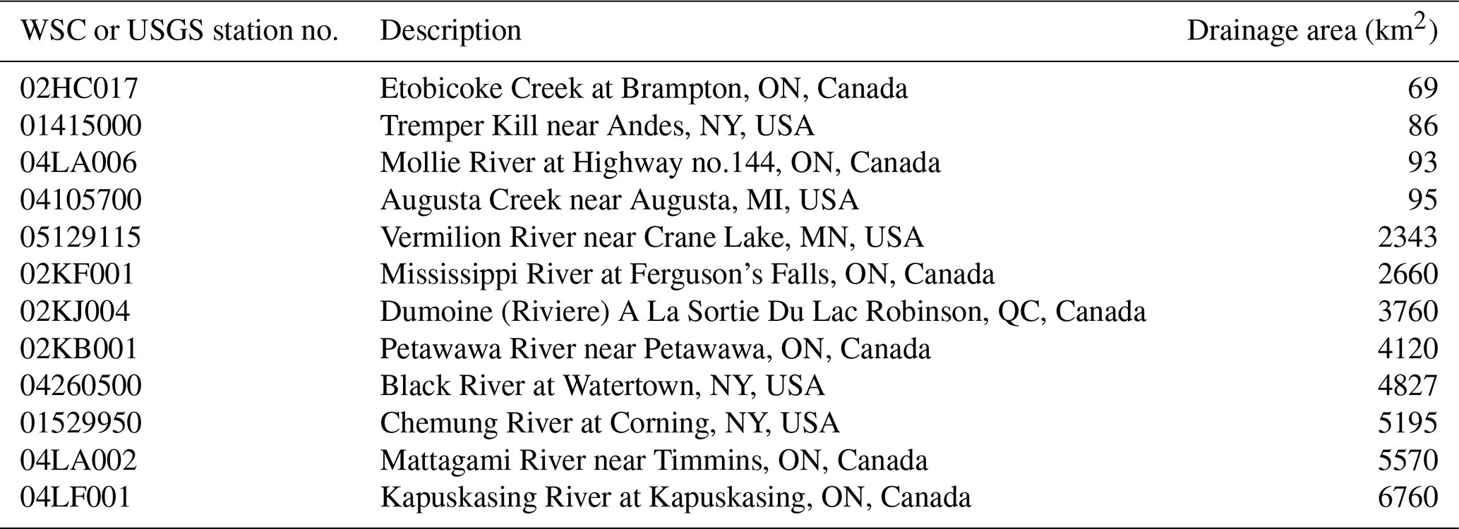
Table 1 Summary of the 12 Non-GRIP-GL gauging basins selected for this study.

2.2 Selection of additional gauging locations for concept validation

We posit that the effective scale of LSTM prediction (i.e., generalizability to various watershed sizes) might be affected by the range and distribution of the drainage area of the training/calibration basins, due to the variation in streamflow patterns in watersheds with different sizes. For instance, hydrological responses in small watersheds tend to be raging and flashy (Camera et al., 2020). The lumped LSTM was trained exclusively on basins with a drainage area exceeding 200 km², in accordance with the selection criteria of gauging basins in the GRIP-GL project. Considering the watershed delineation schemes (GRIP-GL routing and simplified NALRP) deployed in this study, many of the delineated subbasins would have a drainage area smaller than 100 km². Furthermore, the GRIP-GL basins show a skewed distribution in terms of size, with 109 of the 141 calibration basins having a drainage area of between 200 and 2000 km². Similarly, 56 of the 71 validation basins fall within this range. To assess the LSTM performance at the subbasin level (smaller than 200 km²) and for larger watersheds (greater than 2000 km²), we selected 12 additional gauging basins (not used in the GRIP-GL) in the Great Lakes region (within the bounding box defined by the minimum and maximum latitudes and longitudes of the GRIP-GL drainage basin) for spatial and spatiotemporal validation. These basins (summarized in Table 1) include four small basins with a drainage area below 100 km² and eight large basins ranging in size from 2000 to 7000 km².

All Non-GRIP-GL gauged basins are selected based on the following additional criteria:

1. the basin is not heavily regulated by dams or reservoirs;

2. the basin has less than 5 % of missing data in streamflow observation for the study period;

3. the gauge ID at the basin outlet is included in NALRP and, thus, defines a pre-existing routing network.

These criteria, along with the obvious requirement that none of the 212 existing GRIP-GL gauges could be used as additional testing basins, functioned to eliminate more than 1000 streamflow gauges in the region from consideration and, hence, resulted in a relatively small sample size of additional test basins.

2.2.1 Comparison of different routing structures

This analysis aims to investigate the sensitivity of the SR model prediction quality to the chosen delineation method (i.e., the routing network source and spatial resolution). BasinMaker post-processing functions were applied to simplify the initial NALRP routing network for the eight large Non-GRIP-GL basins. Firstly, small lakes were removed using the same minimum lake area threshold as that used for the GRIP-GL routing product (5 km²). Secondly, subbasins were merged by specifying the MDA threshold. For each basin, we delineated seven routing networks, which are defined as follows:

1. Mimic GRIP-GL routing – the same discretization strategy as the GRIP-GL routing product;

2. NALRP_10 % – MDA threshold is calculated as 10 % of each basin's total drainage area;

3. NALRP_100 – MDA threshold is 100 km² for all basins;

4. NALRP_300 – MDA threshold is 300 km² for all basins;

5. NALRP_500 – MDA threshold is 500 km² for all basins;

6. NALRP_800 – MDA threshold is 800 km² for all basins;

7. NALRP_1000 – MDA threshold is 1000 km² for all basins.

2.3 Performance metrics

In this study, the KGE (Gupta et al., 2009) is used to evaluate the performance of the lumped LSTM model and the proposed SR model. The KGE measures the degree of correspondence between two time series (e.g., observations versus a model prediction of those observations). Here, it is computed for daily average streamflow time series and is defined as follows:

$$\begin{array}{}\text{(1)}& \mathrm{KGE}=\mathrm{1}-\sqrt{(r-\mathrm{1}{)}^{\mathrm{2}}+(\mathit{\beta }-\mathrm{1}{)}^{\mathrm{2}}+(\mathit{\alpha }-\mathrm{1}{)}^{\mathrm{2}}},\end{array}$$

where r is the Pearson correlation coefficient, which measures the linear correlation between the observed time series and predicted time series; β denotes the bias term, which indicates whether the model is prone to overestimate or underestimate the streamflow; and α  denotes error in flow variability. The range of the KGE is $(-\mathrm{\infty },\mathrm{1}]$, where KGE = 1 signifies a perfect prediction. It is common to use KGE = 0 as the threshold for determining whether a model exhibits good predictive performance (Knoben et al., 2019). On the other hand, in the GRIP-GL project paper, Mai et al. (2022a) carefully argued that a KGE less than 0.48 would generally be considered a poor model and that models with higher KGE values are of medium or higher quality.

2.4 Experimental design

Three sets of experiments are used to evaluate the quality of the SR model. The first experimental set involved implementing the SR model using the four small Non-GRIP-GL basins. The main objective of this task was to validate the predictive capabilities of the lumped LSTM model with respect to estimating streamflow at a local subbasin-level (LSTM extrapolation to small basins). This was conducted by testing the lumped LSTM on basins that are much smaller than the minimum drainage area in the training dataset. Additionally, we also implemented a single-subbasin routing model in Raven to ensure that our approach to push local streamflow into Raven worked as expected.

In the second set of experiments, we utilized the SR model to predict streamflow on the 212 GRIP-GL basins. This task aims to evaluate the overall performance of the SR model compared with the lumped LSTM. Following the evaluation scheme of the GRIP-GL project, the KGE was calculated separately for temporal validation (trained locations and untrained period), spatial validation (untrained locations and trained period), and spatiotemporal validation (untrained locations and untrained period). Moreover, for validation basins (untrained locations), we calculated the KGE for the whole study period (2001–2017). As mentioned earlier, only the GRIP-GL common routing product was used as the routing structure in this task.

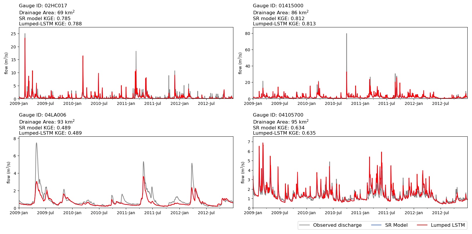
Figure 3 Comparison of observation (grey), lumped LSTM prediction (red), and SR model prediction (blue) for the four small Non-GRIP-GL basins. KGE values over the period from 2001 to 2017 are given for each basin.

For the third set of experiments, the SR model was applied to the eight large Non-GRIP-GL basins. These basins are equivalent to the validation basins in the GRIP-GL project, where we had no previous knowledge or experience applying the LSTM. Each basin was tested with the seven routing structures described in Sect. 2.2.1, in order to investigate the impacts of using alternative routing networks. Note that these routing networks derived from the MERIT DEM differ from those in the second set of experiments, which were derived from the HydroSHEDS DEM, as described in Sect. 2.1.2.

For all experiments, the KGE metric was calculated for the lumped LSTM model predictions and for the semi-distributed SR model predictions, respectively. The lumped LSTM is the benchmark model for comparison with the integrated SR model.

3 Results and discussion

Regarding all hydrographs (line plots) in this section, only the data from January 2009 to December 2012 were plotted (i.e., 2 years in the calibration period and 2 years in the validation period) for better visualization, and the displayed KGE for each basin was calculated for the whole study period (2001–2017). Note that the lumped LSTM and SR models both make predictions starting from the year 2001, as their LSTM models take the year 2000 as the initial input sequence.

3.1 Extrapolating LSTM to small Non-GRIP-GL basins

The lumped LSTM prediction quality for the four small basins (69–95 km²) is quite good, with KGE values for these new test locations of 0.785, 0.812, 0.634, and 0.489, respectively. These KGE values compare favourably with the median GRIP-GL validation performance level of 0.767 reported in Mai et al. (2022a) for the same LSTM applied to much larger basins. Figure 3 shows the daily observed streamflow and the respective predicted streamflow from the lumped LSTM and SR model at each of these four small basins. The predictions from the SR model (blue) are not visible because, as expected, they are the virtually the same as the predictions from the lumped LSTM (red). This can be explained by the fact that the delineation is geometrically identical to the basin outline (i.e., no spatial discretization and each basin is only a single subbasin). In the routing simulation, the LSTM-predicted subbasin streamflow would be directly flushed without delay to the basin outlet, making it equivalent to a lumped prediction.

Overall, these results indicate that the lumped LSTM adequately extrapolates to much smaller basins than those it was trained for and that the translation of LSTM-predicted streamflow into the routing model is correct.

Table 2 Median KGE for the predictive performance of the lumped LSTM and the SR models. The top performing model is indicated by bold font.

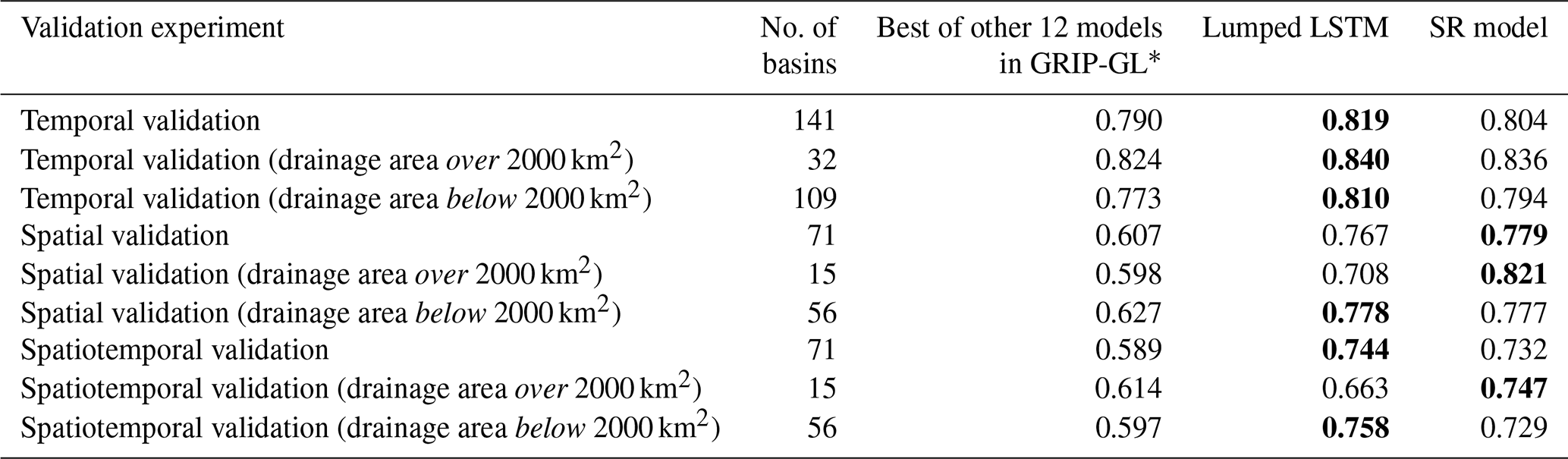
^∗ The 12 models are physically based/physically inspired models.

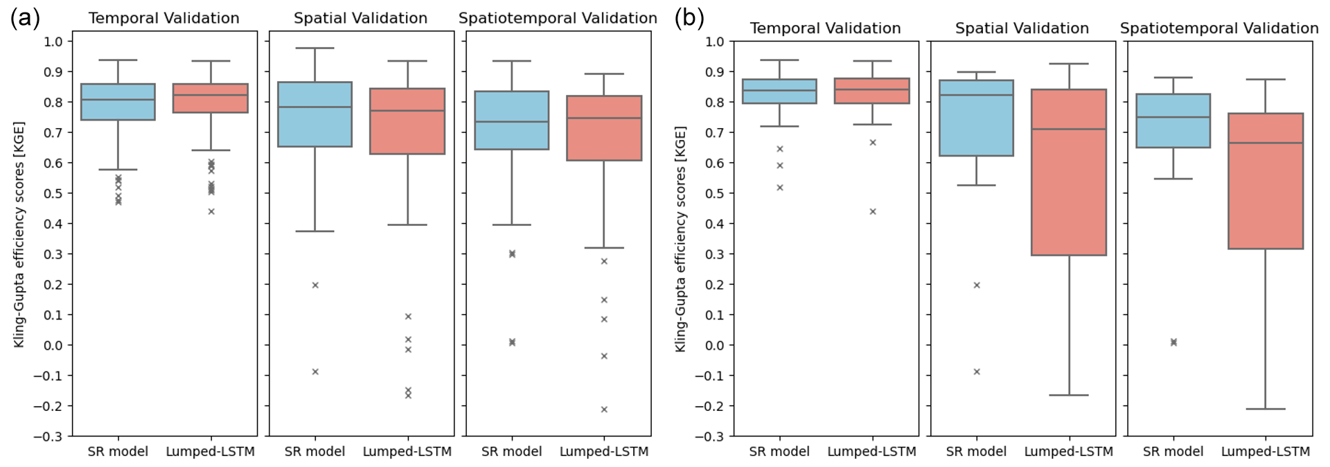
Figure 4 Box plots of KGE validation scores for the SR model (blue) and the lumped LSTM (red): (a) the results of all basins participating in each validation experiment; (b) the results of basins with a size larger than 2000 km².

3.2 Comparing the lumped LSTM and the SR model on GRIP-GL basins

The SR modelling approach should be able to outperform the lumped LSTM for basins with large drainage areas, as spatially distributed modelling will mitigate the information loss caused by feeding the lumped LSTM with basin-averaged features, and the SR model will take advantage of maintaining such spatial heterogeneity. Therefore, the results are evaluated in two ways: results first include all basins (corresponding to the validation experiment in the GRIP-GL study), while the second way focuses solely on basins larger than 2000 km².

The performance results of the lumped LSTM and the SR model for GRIP-GL basins are summarized in Table 2 and visually compared in Fig. 4. In the temporal validation experiment, the SR model predictions shows a comparable level of quality to those of the lumped LSTM. The interquartile range of the lumped LSTM is slightly narrower than that of the SR model, suggesting less variability in the KGE score distribution. The results indicate that the lumped LSTM better captures the temporal trends and seasonal patterns at trained locations, while the SR model, relying on an uncalibrated process-based routing model, shows no improvement (slightly reduced KGE values) relative to the lumped LSTM results for both large (> 2000 km²) and small (< 2000 km²) basins. However, the SR model results for all basins are better than the best of 12 physically based/physically inspired GRIP-GL hydrological models (see Table 2).

In the spatial validation and spatiotemporal validation experiments, both the SR model and the lumped LSTM exhibit similar performance degradation relative to temporal validation performance (considering all basins). These two experiments primarily focus on assessing the models' robustness with respect to predicting streamflow in an ungauged basin scenario (where no local streamflow observations were used to train the model). It is worth mentioning that the LSTM prediction at each subbasin is practically also a prediction of streamflow in an ungauged basin (refer to the first task described in Sect. 3.1).

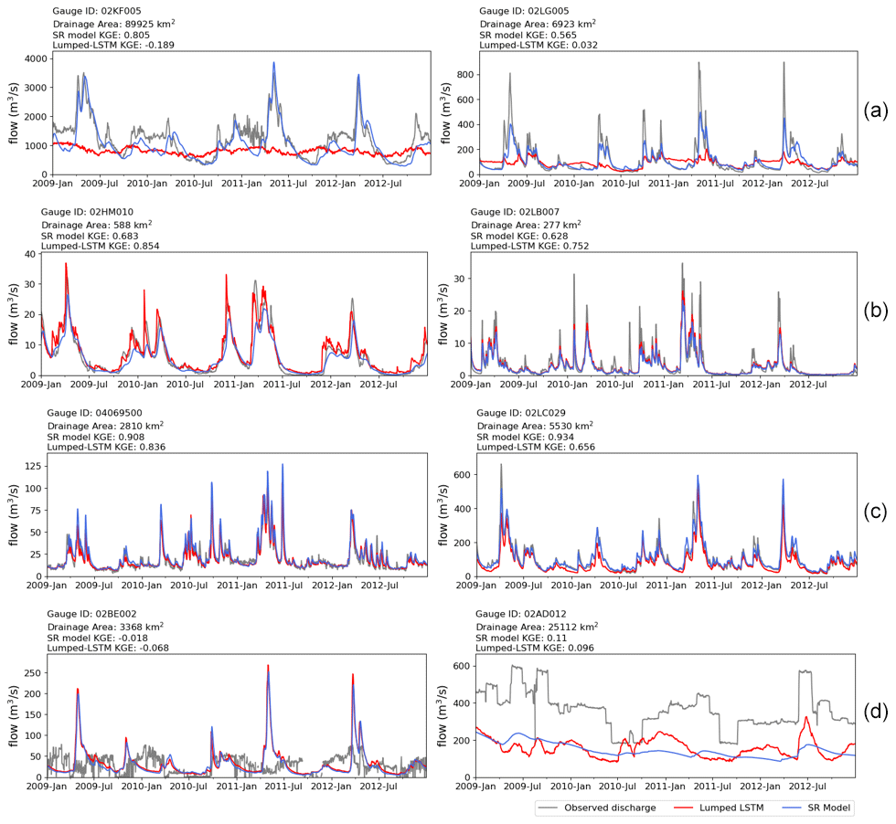
Figure 5 Comparison of time series of observation (grey), lumped LSTM prediction (red), and SR model prediction (blue) for representative GRIP-GL validation basins, over the selected period from 2009 to 2012. KGE values over the whole study period from 2000 to 2017 are given for each basin. (a) The two basins that show the most significant improvement compared with the lumped LSTM. (b) The two basins that show the most significant degradation compared with the lumped LSTM. (c) The two basins where the SR model achieves the highest KGE scores. (d) The two basins where the SR model achieves the lowest KGE scores.

As with the temporal validation, when considering all basins in spatial or spatiotemporal validation, the SR model shows no real difference in median KGE values relative to the lumped LSTM results. However, the advantage of the SR model in larger basins becomes apparent in these untrained locations. Compared with the lumped LSTM, for large basins over 2000 km², the median KGE of the SR model is 0.113 KGE units higher for the spatial validation and 0.084 KGE units higher for the spatiotemporal validation. These improvements for large basins came with no real performance drops for small basins (< 2000 km²), as the median KGE values for both the SR model and the lumped LSTM were within 0.030 KGE units difference across all three validation modes (0.016 for temporal validation, 0.001 for spatial validation, and 0.029 for spatiotemporal validation). Furthermore, the SR model results are substantially better than the best of 12 physically based/physically inspired GRIP-GL hydrological models for all basins. This is notable given that 7 of these 12 models in GRIP-GL were spatially distributed (not lumped) and utilized the same routing network discretization as the SR model for each basin.

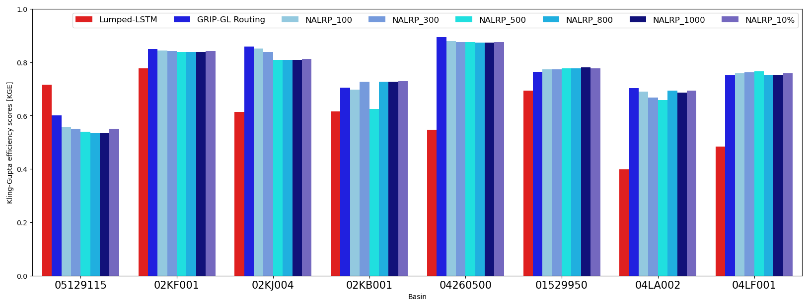
Figure 6 Overall model performance when adopting different routing network delineations in the eight large Non-GRIP-GL basins, during the whole study period 2000–2017. The basins are sorted (from left to right) in ascending order according to size, from smallest (2343 km²) to largest (6760 km²).

Figure 5 displays the time series of observations, model predictions, and KGE scores for representative GRIP-GL validation basins. Figure 5a shows the hydrographs of the two basins where the SR model demonstrates the largest improvement (better by more than 0.5 KGE units) compared with the lumped LSTM. Among them, 02KF005 (Ottawa River at Britannia) is the largest basin studied in the GRIP-GL project, with an almost 90 000 km² drainage area. The other basin is approximately 6923 km² in size (WSC gauge 02LG005, Gatineau Riviere Aux Rapides Ceizur). The deficiency in the lumped LSTM model is evident, as it fails to capture the peaks and seasonal variations in these two large watersheds and predicts constantly low flow throughout the study period. Figure 5b compares hydrographs at WSC gauges 02HM010 (Salmon River at Tamworth) and 02LB007 (South Nation River at Spencerville), where the prediction accuracy of the SR model shows the worst degradation relative to the lumped model (by 0.17 and 0.12 KGE units, respectively). These two gauges are small (588 km² broken into nine subbasins in the SR model and 277 km² broken into three subbasins in the SR model) and within the range of training basin sizes. It is important to note that the spatial resolution of the CaSR-v2 dataset is 10 km  × 10 km; thus, each grid covers an area of approximately 100 km², and breaking these small basins up into a handful of smaller subbasins is likely unnecessary in terms of representing the spatial rainfall patterns. In general, the SR model aligns with the overall pattern of the observed streamflow, but it tends to underestimate peak flows, and the lumped LSTM predicts larger peaks for these small basins. This underestimation of peak flow events is not evident in most of the high-quality SR model hydrographs; in fact, in the larger two basins shown in Fig. 5c, the SR model predicts higher peaks than the lumped LSTM. Figure 5c shows the two basins where the SR model achieves the highest KGE scores (both over 0.9 and both large basins), and these are both notably improved over the lumped LSTM. The hydrographs of two basins where the SR model achieves the lowest KGE scores (both around 0) are shown in Fig. 5d. It is evident that both the lumped LSTM and the SR model were unable to simulate flow in these basins, which, according to the observed hydrograph, appear to be substantially impacted by regulation. The failure of both models in regulated basins is not surprising given that none of the LSTM attributes measure or indicate the degree of regulation within a basin.

3.3 New testing basins and the impact of routing network delineation

Eight large basins (not used in the GRIP-GL study) were identified as suitable additional independent testing basins according to the criteria in Sect. 2.2 in order to conduct further comparisons between the lumped LSTM and the SR model built with varying routing networks. Like the GRIP-GL validation basins, neither model was trained on these eight new basins.

Figure 6 summarizes the comparative results and shows the KGE of each model in each of the eight basins. From Fig. 6, it can be seen that the choice of the delineation method (routing network resolution) has a minor impact on predictive performance. In general, the differences in overall KGE scores among the seven different resolution routing networks are not significant at each basin. This could be attributed to the consistent representation of lakes across all of the routing networks (all resolutions retain lakes more than 5 km² in area in the network) combined with the crucial role that these lakes play in modelling the transport of water.

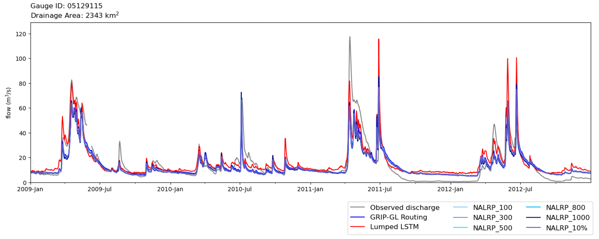
Figure 7 Comparison of the time series of observation (grey), lumped LSTM prediction (red), and SR model predictions with different routing networks for the Vermilion River basin 05129115. Note that the lines of NALRP time series all follow extremely similar trends to the GRIP-GL routing series and, thus, are not distinguishable.

In terms of relative model performance, the SR model outperforms the lumped LSTM model in seven of the eight tested basins (improved by an average of 0.160 KGE units, using the GRIP-GL routing network resolution). This result strongly reinforces the findings in Sect. 3.1, showing that the SR model tends to exhibit better relative performance in basins with larger drainage areas. The SR model achieved the worst KGE score in the basin identified by the USGS gauge 05129115 (Vermilion River near Crane Lake), and this is the only basin where the lumped LSTM (KGE score of 0.716) outperformed the SR model (KGE scores from 0.534 to 0.600). As depicted in Fig. 6, the KGE scores at this basin exhibit a gradual decrease as the resolution of the routing network becomes coarser, such as with NALRP_800 and NALRP_1000. Figure 7 shows the hydrographs for USGS gauge 05129115; while it is evident that the SR model successfully captures the timing of the peaks, it consistently underestimates their magnitude in comparison with the observations and the lumped LSTM.

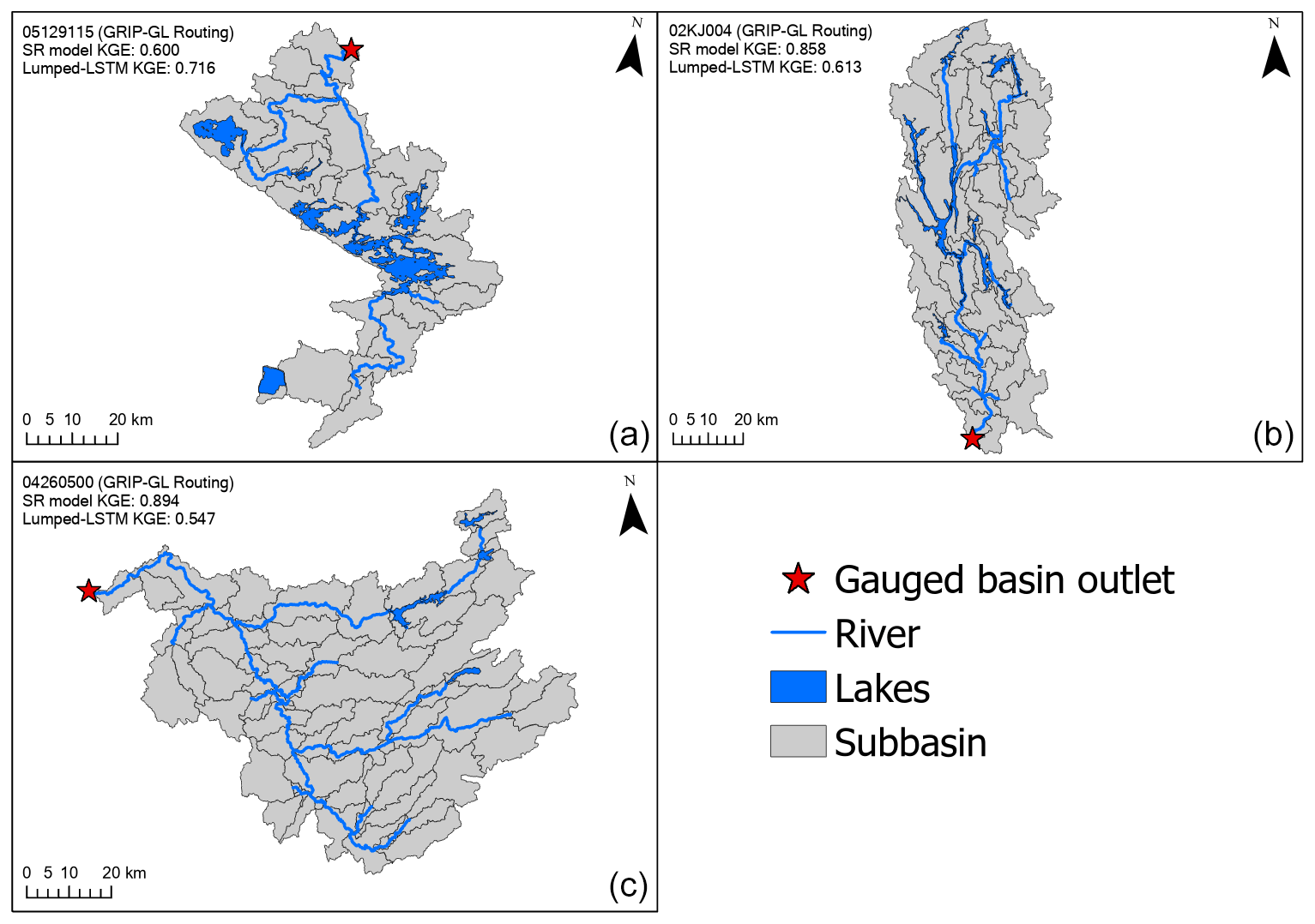
Figure 8 Comparison of the routing networks of three large Non-GRIP-GL basins to illustrate the variation in different lake densities: (a) gauged basin 05129115 (5 lakes, 14 % of the basin is covered by lakes); (b) gauged basin 02KJ004 (11 lakes, 10 % of the basin is covered by lakes); (c) gauged basin 04260500 (4 lakes, 4 % of the basin is covered by lakes). The three illustrated routing networks were delineated to mimic the GRIP-GL routing delineation strategy.

The degradation in performance could be attributed to the heavy presence of lakes within this basin (as shown in Fig. 8a). Among the eight tested basins, 05129115 stands out with the largest fraction of its area covered by lakes, accounting for approximately 14 % of its total area. In contrast, the SR model shows significant improvement in basin 02KJ004, which has the second highest proportion of lake coverage, approximately 10 % (as depicted in Fig. 8b). However, the lake areas are vastly different in these two basins. Lakes in 05129115 are mainly concentrated as one very large lake in the middle of the basin, whereas the lakes in 02KJ004 are more numerous, smaller, and generally long and narrow. On the other hand, the SR model shows a substantial improvement over the lumped LSTM (by over 0.347 KGE units) in a lake-sparse basin gauged by USGS station 04260500 (see Fig. 8c). Notably, this is also the additional testing basin where the SR model achieved the highest KGE score of 0.894.

4 Conclusions

In this study, we proposed a hybrid modelling approach named the Spatially Recursive (SR) model that aims to enhance the accuracy of streamflow predictions made by lumped data-driven models. For a basin of interest, a regionally trained lumped LSTM is used to predict the local streamflow at the subbasin level (as delineated in the basin's lake–river routing network), and a process-based hydrological routing-only model then simulates the transport of local streamflow from the subbasin outlet to the basin outlet. The novelty of the SR model is threefold: (1) it considers the spatial variability in input variables at finer spatial resolution by having smaller response units than the training dataset (i.e., in our case, this is from the basin scale to the subbasin scale); (2) it integrates physically based lake–river hydrological routing with data-driven learning to form a generalizable modelling approach for enhanced streamflow prediction in large, ungauged basins; (3) it operates without the need for further fine-tuning, parameter transfer, or training/calibration, given that the trained LSTM is available.

Three sets of experiments were conducted to examine the applicability and performance of the SR model. First, we validated the concept of predicting streamflow at the local subbasin-level with an LSTM trained using much larger basins. This was done by predicting streamflow at four small testing basins (< 100 km²) which were used as mimic local subbasins. The results revealed that the lumped LSTM can indeed be applied to predict streamflow in basins below the minimum drainage area threshold of the training dataset.

Subsequently, the SR model was evaluated on 212 basins from the GRIP-GL project. The results showed that the SR model is comparable to lumped LSTM in terms of overall performance across basins of all drainage areas. The SR model exhibits a noticeable advantage with respect to predicting streamflow in large basins (> 2000 km²), which demonstrates that incorporating spatially distributed inputs can be beneficial to the hydrological modelling in large basins, due to the fact that the spatial heterogeneity is naturally more significant in larger regions. The empirical performance improvement over the lumped LSTM is most significant in a PUB context. For the 15 large GRIP-GL validation basins, the median KGE levels over the 10-year training period and the 7-year testing period, are 0.11 and 0.08 KGE units higher, respectively, than those of the lumped LSTM. Importantly, for smaller basins (< 2000 km²), the performance gains for large basins do not result in significant performance drops, as the median KGE difference between the SR model and the lumped LSTM were within 0.03 KGE units in all three validation modes.

Lastly, we investigated the impacts of the routing network delineation by testing the SR model in eight additional large basins (2343–6760 km²). This out-of-sample testing showed that the SR model was substantially better (by an average of 0.16 KGE units) than the lumped LSTM for seven of eight basins over the 17-year period. It further corroborated the superiority of our method for modelling large, heterogeneous basins. Results also clearly show that the substantial performance gains of the SR model over the lumped LSTM are not sensitive to a range of routing network configurations, and these performance gains occur in basins with both large and small fractions of the basin covered by lakes.

Moreover, these improvements in the SR model relative to the lumped data-driven model did not require calibration or additional training after the original lumped LSTM was trained. In fact, the reported results of the SR model reflect a conservative estimate (i.e., lower bound) of performance, considering the following factors: (1) the regional LSTM within the SR model could be improved with additional training data (Kratzert et al., 2024); (2) the SR model routing parameters could be calibrated and regionalized to further improve validation results; and (3) the regional LSTM could be purpose-built to train on a sufficient number of small basins better matching the subbasin-level spatial scale at which the lumped LSTM would be applied within the SR model (e.g., 131 km² as the average subbasin size of the GRIP-GL routing product).

The findings of this study highlight the importance of considering spatially distributed inputs to streamflow prediction and demonstrate a new way that data-driven models can benefit from such information. This research opens up new avenues for future research regarding hybrid modelling in hydrology, by improving an existing data-driven model with an uncalibrated hydrological routing approach. The simplicity of our approach, combined with the explosive growth of regionally trained LSTM models for streamflow prediction, means that our approach should be accessible to all hydrological modellers. Future refinement of the proposed SR modelling approach could focus on two key aspects: the training strategy of the lumped data-driven predictor (e.g., larger dataset, targeted training basin sizes, and different neural networks) and the calibration of hydrological-routing-related parameters.