A framework for parameter estimation, sensitivity analysis, and uncertainty analysis for holistic hydrologic modeling using SWAT+

Parameter sensitivity analysis plays a critical role in efficiently determining main parameters, enhancing the effectiveness of the estimation of parameters and uncertainty quantification in hydrologic modeling. In this paper, we demonstrate an uncertainty and sensitivity analysis technique for the holistic Soil and Water Assessment Tool (SWAT+) model coupled with new gwflow module, spatially distributed, physically based groundwater flow modeling. The main calculated groundwater inflows and outflows include boundary exchange, pumping, saturation excess flow, groundwater–surface water exchange, recharge, groundwater–lake exchange and tile drainage outflow. We present the method for four watersheds located in different areas of the United States for 16 years (2000–2015), emphasizing regions of extensive tile drainage (Winnebago River, Minnesota, Iowa), intensive surface–groundwater interactions (Nanticoke River, Delaware, Maryland), groundwater pumping for irrigation (Cache River, Missouri, Arkansas) and mountain snowmelt (Arkansas Headwaters, Colorado).

The main parameters of the coupled SWAT+gwflow model are estimated utilizing the parameter estimation software PEST. The monthly streamflow of holistic SWAT+gwflow is evaluated based on the Nash–Sutcliffe efficiency index (NSE), percentage bias (PBIAS), determination coefficient (R²) and Kling–Gupta efficiency coefficient (KGE), whereas groundwater head is evaluated using mean absolute error (MAE). The Morris method is employed to identify the key parameters influencing hydrological fluxes. Furthermore, the iterative ensemble smoother (iES) is utilized as a technique for uncertainty quantification (UQ) and parameter estimation (PE) and to decrease the computational cost owing to the large number of parameters.

Depending on the watershed, key identified selected parameters include aquifer specific yield, aquifer hydraulic conductivity, recharge delay, streambed thickness, streambed hydraulic conductivity, area of groundwater inflow to tile, depth of tiles below ground surface, hydraulic conductivity of the drain perimeter, river depth (for groundwater flow processes), runoff curve number (for surface runoff processes), plant uptake compensation factor, soil evaporation compensation factor (for potential and actual evapotranspiration processes), soil available water capacity and percolation coefficient (for soil water processes). The presence of gwflow parameters permits the recognition of all key parameters in the surface and/or subsurface flow processes, with results substantially differing if the base SWAT+ models are utilized.

1 Introduction

Hydrologic models have been developed to enhance our understanding of the dynamics of hydrological fluxes to address practical issues related to water resource management (Liu et al., 2020; Wei et al., 2018), especially under the influence of anthropogenic activities and climate change, which can result in significant changes in the hydrological system (Abbas et al., 2022; Pokhrel et al., 2021). Typically, hydrologic models include several parameters to represent the hydrologic processes and to consider spatial variations resulting from climate, soil type, land use, etc. (Fatichi et al., 2016; Čerkasova et al., 2021).

To employ hydrologic models in a responsible manner for system understanding and scenario analysis, sensitivity analysis (SA), uncertainty analysis (UA) and parameter estimation (PE) are key steps in the modeling process due to the presence of spatial heterogeneities (Bennett et al., 2013; Doherty and Hunt, 2009) and, often, the use of a broad suite of model parameters. SA identifies model parameters that have a strong influence on model output (e.g., streamflow), and results generally can provide insights into system behavior and point to system parameters that require more data collection or management strategies that may be efficient in controlling a certain system response (Leta et al., 2015). UA relates uncertainty in model parameters to model output and hence can provide ranges of system output possibilities, e.g., when using the model in scenario analysis as a decision support tool, to answer questions regarding the effects of system changes. PE provides the best values for matching model predictions to historical observations.

SA methods can be classified into local sensitivity analysis (LSA) and global sensitivity analysis (GSA) (Santos et al., 2022). Examples of LSA approaches are the one-variable-at-a-time (OAT) method and the differential analysis (DA) method (Devak and Dhanya, 2017); these are less reputable since they disregard considering the interaction between several parameters and cannot precisely estimate optimal parameters value (Helton, 1993). On the other hand, GSA techniques such as regional sensitivity analysis (RSA), Morris screening, variance-based sensitivity analysis (the Sobol method) and the Fourier amplitude sensitivity test (FAST) have been developed and used in many applications (Olaya-Abril et al., 2017; Devak and Dhanya, 2017). These methods take into account the interaction between different parameters by altering several parameters of models together (Pianosi et al., 2017; Devak and Dhanya, 2017). GSA is gaining prominence in hydrologic and environmental modeling (e.g., Plischke et al., 2013; Pianosi et al., 2017). GSA is employed for the detection of insignificant parameters and the identification of influential parameters with a significant impact on model outputs (Santos et al., 2022).

Other GSA applications include identification of model behavior, prioritization for uncertainty estimation and reduction, and for simplification of the model (Pianosi et al., 2017). However, these methods typically require a large number of model evaluations. More recently, iterative ensemble smoother (iES) techniques have been developed for uncertainty quantification (UQ) and for more efficient parameter estimations (PE) by reducing the number of model evaluations incurred by large numbers of parameters (Chen and Oliver, 2012); this technique can be implemented in a non-intrusive and/or model-independent approach, resulting in a desirable option for application to analyses of hydrologic and environmental modeling. The iES has been utilized in several applications (e.g., Bocquet and Sakov, 2014; Crestani et al., 2013).

The null-space Monte Carlo approach (NSMC) is not dissimilar to the iES approach in their goals: to represent posterior parameter uncertainty, especially as it relates to null-space parameters and parameter components (i.e., non-unique parameters). However, NSMC uses a full-rank Jacobian filled using finite-difference perturbations, linearized at the final calibration parameter set to project a prior parameter ensemble, realization by realization, toward being calibrated under the assumption of linearity. In contrast, the iES approach propagates the prior parameter ensemble directly during history matching and avoids filling a full-rank Jacobian, instead using an ensemble approximation of the Jacobian, an approximation that is more regional or even global compared to the linearized local Jacobian used in the NSMC. Because of this, ensemble methods can, in general, cope with higher levels of nonlinearity in the relation between parameters and observations and can also scale to much larger numbers of parameters (since the relation between the number of parameters and number of model runs is removed).

Although SA–UA–PE methods have been applied numerous times to watershed models such as SWAT (Arnold et al., 1998) (e.g., Pianosi et al., 2017; Nossent et al., 2011; Qiu et al., 2019), their application to coupled surface–subsurface models is sparse (e.g., Herzog et al., 2021; Wu et al., 2014; Ryken et al., 2020). For example, the coupled SWAT-MODFLOW model (Bailey et al., 2016) has been applied to regions worldwide (e.g., Izady et al., 2022; Abbas et al., 2022; Sith et al., 2019), and more recently, the SWAT+ model (Bieger et al., 2017) with the gwflow module (Bailey et al., 2020) has been applied to simulate hydrological processes in watershed systems; but these models have been applied without SA and in a deterministic manner, i.e., without including UA. In addition, PE has been challenging, with SWAT and MODFLOW often being calibrated separately before being linked, which can be attributed to the complexity in the interaction between SWAT and MODFLOW, as well as the high dimensionality of the parameter space of these two models.

In this paper, we demonstrate the use of SA, PE and UA methods in a coupled SWAT+gwflow model to identify surface and subsurface parameters that control two key watershed responses: streamflow and groundwater head. Hydrologic fluxes in the coupled model include vegetation ET, surface runoff, infiltration, soil percolation and recharge, saturation excess flow, groundwater–stream exchange, soil lateral flow, groundwater pumping, groundwater–lake exchange, tile drainage outflow, and boundary exchange. Targeted parameters include soil properties, evaporation parameters, runoff curve number, snow parameters, aquifer properties (hydraulic conductivity, specific yield), streambed properties (hydraulic conductivity, thickness) and tile drain parameters. The chosen SA method is the Morris screening method, joined to a PE method using the PEST (Parameter ESTimation Tool) software program (Doherty, 2020). In an alternate method, we demonstrate the use of UA in the PE process, using an iterative ensemble smoother (iES) to establish prior and posterior ensembles of parameters and system responses. Both methods (PE–SA and iES) can be key components in the application of coupled surface–subsurface models to watershed systems. While, in this paper, we demonstrate methods for the SWAT+gwflow modeling system, they can be applied to other hydrologic models.

We demonstrate the methods for four eight-digit watersheds throughout the conterminous United States: Nanticoke River (Delaware, Maryland), Arkansas Headwaters River (Colorado), Winnebago River (Minnesota, Iowa) and Cache River (Missouri, Arkansas). These watersheds are chosen owing to their distinct hydrologic characteristics, such as their snowmelt-dominant basin (Arkansas Headwaters), their shallow groundwater (Nanticoke), the extensive networks of subsurface tile drains (Winnebago), and groundwater pumping for irrigation (Cache). The SWAT+gwflow models were simulated for each watershed from 2000 to 2015, with a 2-year warm-up period (2000–2001), 7-year calibration period (2002–2008) and 7-year testing period (2009–2015). These models were tested based on annual groundwater head and measured monthly streamflow measured at USGS monitoring wells and stream gages, correspondingly. Preliminary models of SWAT+gwflow for the Winnebago River watershed, the Nanticoke River watershed and the Cache River watershed were presented in Bailey et al. (2023), but only uncalibrated results were provided. This current study establishes possible SA–UA–PE methods to increase model accuracy to a level suitable for scenario analysis (e.g., conservation practices, changes in climate and land use) in these watersheds.

2 Materials and methods

2.1 Modeling framework for the study watersheds

Figure 1 presents four watersheds in United States with different hydrologic features that were selected for SWAT+gwflow simulation: Nanticoke River (Delaware, Maryland), Arkansas Headwaters River (Colorado), Winnebago River (Minnesota, Iowa) and Cache River (Missouri, Arkansas). A comprehensive summary of the primary characteristics of each watershed is presented in Table 1. The annual precipitation rates vary between 425 mm (Arkansas Headwaters) to 1287 mm (Cache), while the total surface area of the watersheds varies considerably, from 1787 km² for Winnebago to 7940 km² for Arkansas Headwaters. Each watershed is a headwater eight-digit watershed and is in a different two-digit region.

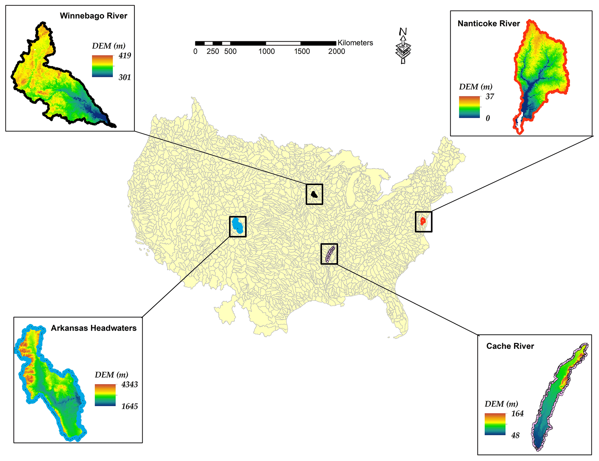
Figure 1 Geographical locations and digital elevation model of the four study watersheds: Arkansas Headwaters River, Winnebago River, Nanticoke River and Cache River.

Table 1 Key features for the four study basins.

These four watersheds were specifically chosen on account of distinctive hydrologic characteristics that demonstrate informative application of the gwflow, such as high baseflow with extensive groundwater discharge to streams (Nanticoke; Wolock, 2003), extensive presence of tile drainage (Winnebago), humid climate (Cache and Nanticoke), semi-arid climate (Arkansas Headwaters), extensive groundwater pumping for irrigation (Cache) and mountain snowmelt (Arkansas Headwaters). A detailed map of the study areas showing watershed boundaries, streams, 12-digit catchment boundaries (i.e., subbasin), USGS river gage stations, USGS groundwater monitoring well locations, weather station locations and water bodies is shown in Fig. 2.

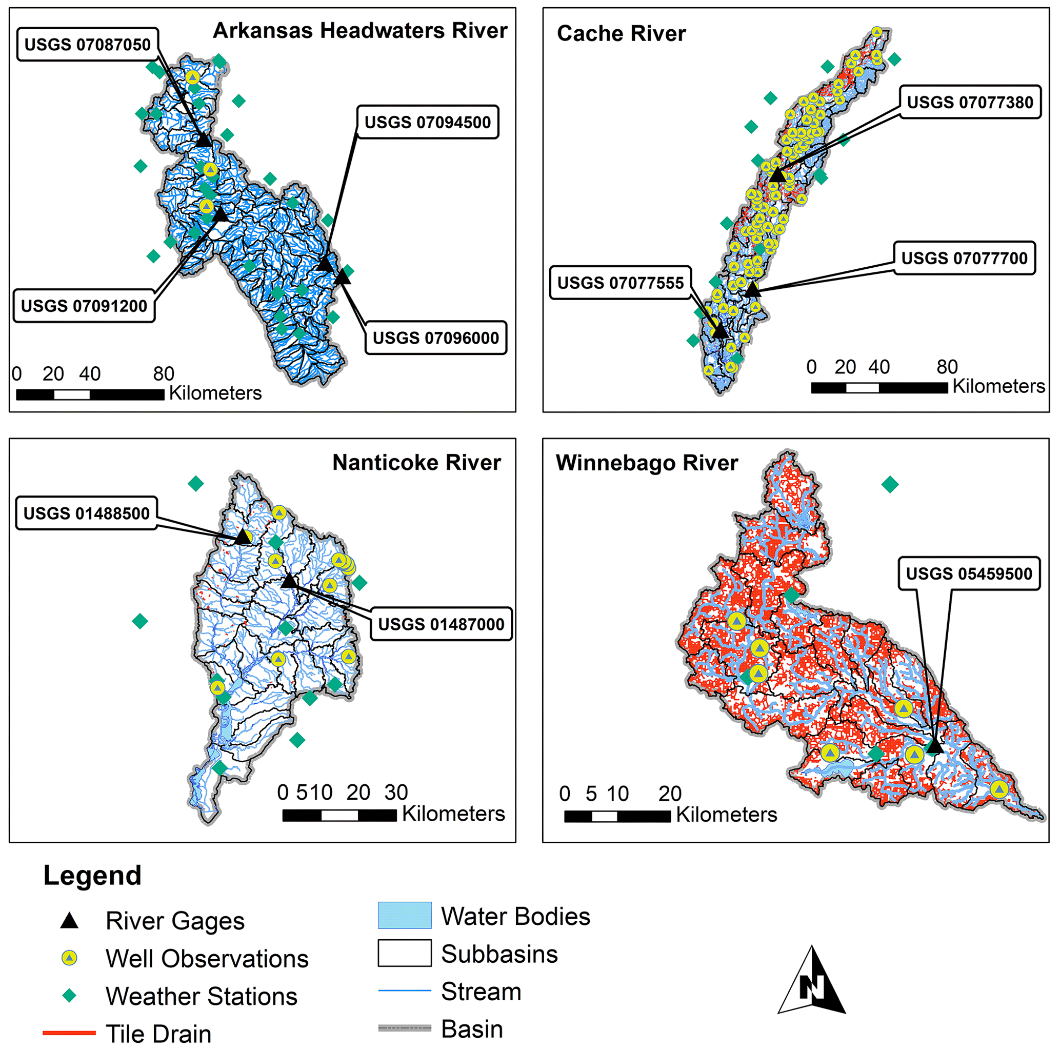
Figure 2 Detailed maps of the study watersheds, revealing the location of water bodies, streams, USGS monitoring wells, weather stations, subbasin boundaries, tile drains and river gage stations.

2.1.1 SWAT+ model

The Soil and Water Assessment Tool (SWAT; Arnold et al., 1998) is a process-based, basin-scale, semi-distributed, continuous-time hydrologic model that has been applied in many countries around the world for watershed management, policy development and environmental planning (Bieger et al., 2015; Zhang et al., 2020). The SWAT model was developed and designed by the Agricultural Research Service (ARS) of the United States Department of Agriculture (USDA) to simulate spatial and temporal variations in processes and fluxes of water, nutrients and sediment. Common uses of the model include assessing water supply, nutrient loads and sediments loads under historical and future conditions of climate, land use and land management practices within watersheds and river basins of varying scale (e.g., Ghaffari et al., 2010; Wang et al., 2018; Bhatta et al., 2019). The main computational unit within SWAT is the hydrologic response unit (HRU), unique geographic areas of soil type, land use and topographic slope (Neitsch et al., 2011), with fluxes aggregated at the subbasin level and then routed to streams. Stream routing occurs from upstream to downstream, with the total watershed yield of water, nutrients and sediment occurring at the watershed outlet.

The SWAT modeling code has recently been restructured to SWAT+ (Bieger et al., 2017), which provides additional flexibility in routing water, nutrients and sediment between watershed spatial objects (HRUs, aquifers, reservoirs, channels, routing units, wetlands). As an example, fluxes can be routed from HRU to HRU or from channel to channel within a single subbasin, whereas the original SWAT only allowed routing from HRUs to channels, and each subbasin had a single channel. However, as with the original SWAT model, the groundwater processes are treated simplistically, assuming steady-state conditions and homogeneous aquifers, and without physically based movement of groundwater and exchange with surface water features using hydraulic head potential and differences. Hence, the gwflow module was created for SWAT+ to allow the representation of groundwater processes and fluxes in a physically based manner (Bailey et al., 2020), as described in Sect. 2.1.2.

In this study, we use SWAT+ models that have been created within the National Agroecosystem Model, NAM (White et al., 2022; Arnold et al., 2020), a national effort for improving environmental assessments and conservation strategies. Within the NAM, a SWAT+ model is constructed for each of the 2139 HUC8 (eight-digit hydrologic unit code) watersheds within the conterminous United States, simulating hydrologic processes and management according to five domains: main rivers (>150 km²), tributaries (15–150 km²), headwaters (1–15 km²), transitions (0.2–2.0 km²) and fields (1–50 ha). Table 2 lists the data sets used to create each SWAT+ model using publicly available data sources. Each cultivated field is designated as a unique HRU, with remaining HRUs delineated based on topographic slope, land use and soil type. Subbasin boundaries coincide with HUC12 catchments within each HUC8 watershed. Each National Hydrography Dataset (NHD+) channel segment is designated as a unique channel in SWAT+. White et al. (2022) provide detailed information on model construction and input data sets. We use these model set-ups for the four study watersheds.

Table 2 Data sets utilized to create the gwflow inputs and the base SWAT+ models (Bailey et al., 2023).

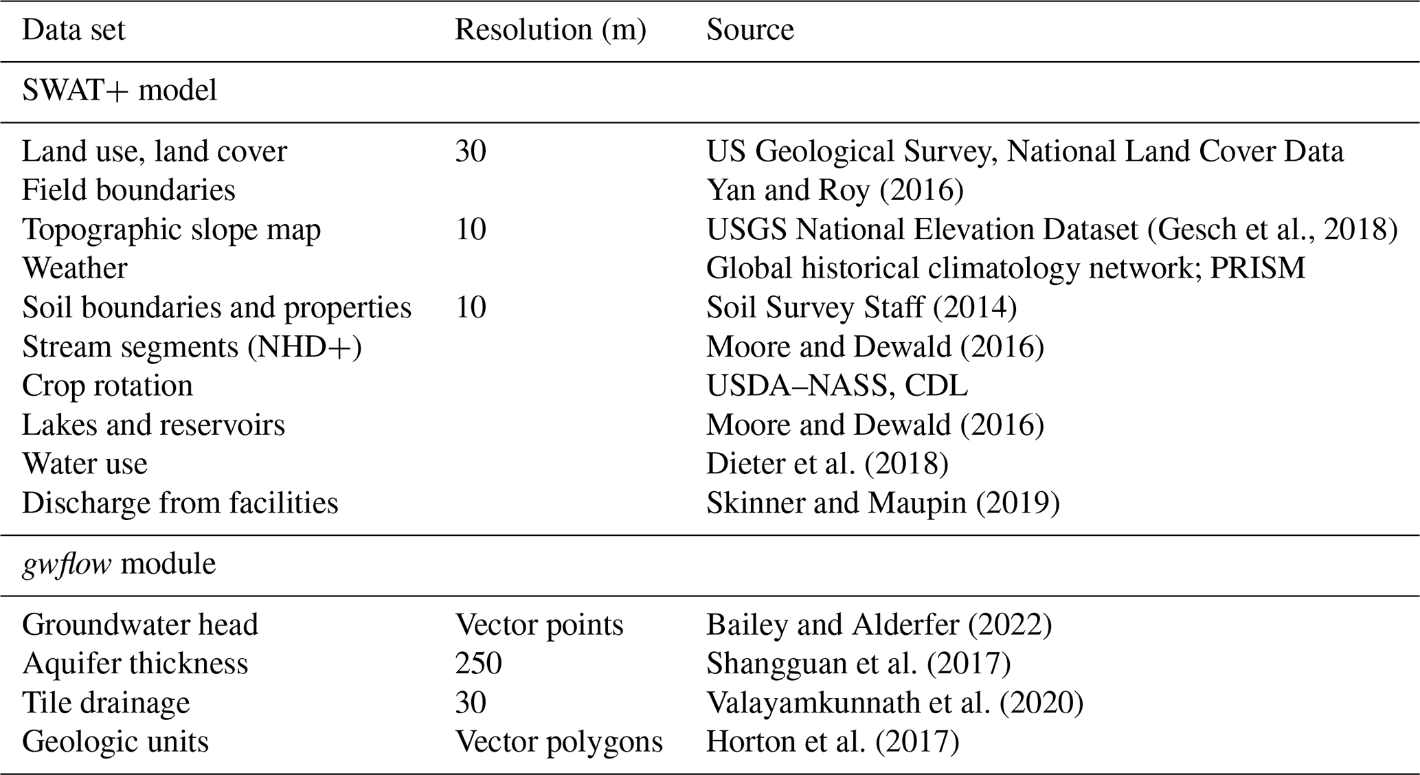
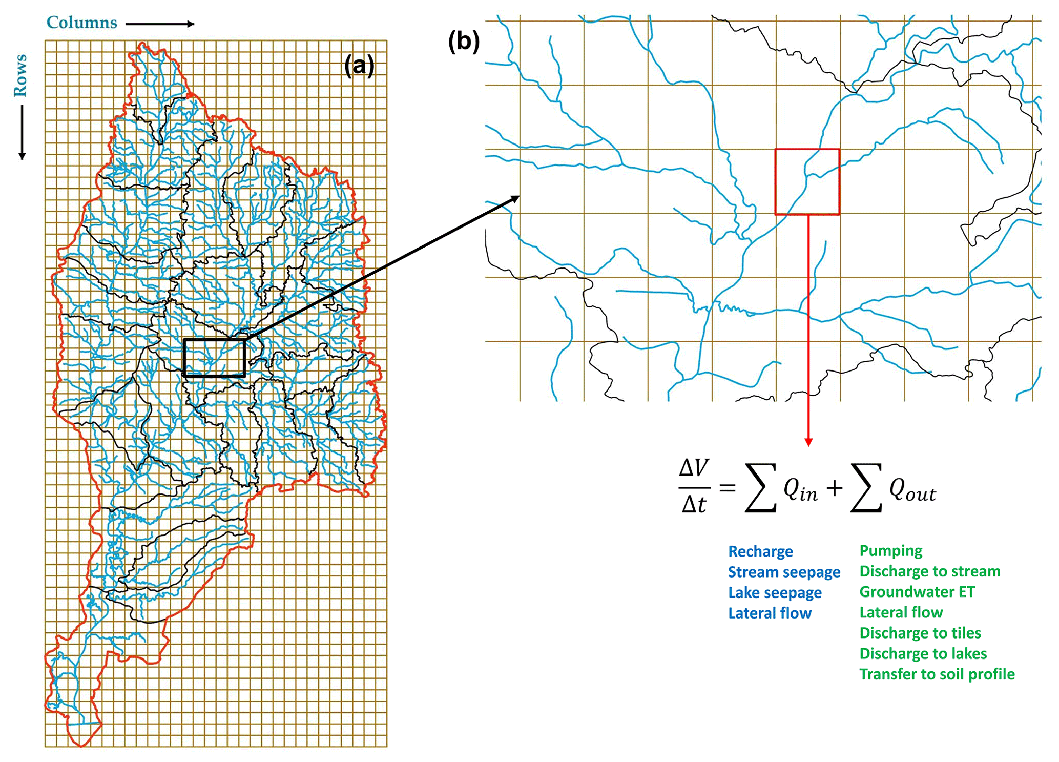
Figure 3 Geographical layout and computation method of the gwflow module, presenting (a) grid cells, watershed boundary (red line), stream channels (blue lines) and subbasins (black lines) for the Nanticoke watershed and (b) zoomed-in section of channels and grid, demonstrating the water balance computations for each cell.

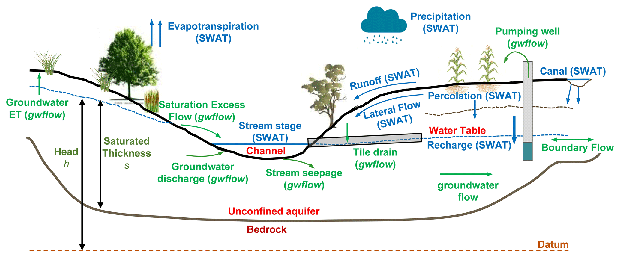
Figure 4 Schematic representation of the hydrologic processes in a typical watershed stream–aquifer system showing the main hydrologic elements and hydrologic processes for SWAT+ and gwflow. Blue arrows outline fluxes that are calculated by SWAT+, and green arrows are for flow processes that are computed by gwflow.

2.1.2 gwflow module

The gwflow module (Bailey et al., 2020, 2023) is constructed and combined with SWAT+ for physically based, spatially distributed groundwater storage and flow modeling in unconfined aquifer systems to replace the original SWAT+ groundwater module. The default SWAT+ groundwater module simulates groundwater fluxes with homogeneous aquifer properties, an absence of groundwater flow between nearby aquifer systems, and groundwater discharge to streams based on aquifer storage and release parameters, acting as a substitute to distributed values of gradients and head differences. If the gwflow module is activated, the routine is called during each daily time step of the simulation; gwflow utilizes a set of grid cells to simulate groundwater storage and flow through time (Fig. 3). Each grid cell has a specified aquifer volume, calculated using the ground surface elevation, bedrock elevation and specific cell widths. Groundwater storage V (m³) is updated during each daily time step (time n to time n+1) for each cell (i, j) using a groundwater balance equation:

$$\begin{array}{}\text{(1)}& \begin{array}{rl}{V}_{i,j}^{n+\mathrm{1}}=& V_{i,j}^n+\left({\mathrm{sources}}_{i,j}^n-{\mathrm{sinks}}_{i,j}^n\mp \mathrm{lateral}{\mathrm{flow}}_{i,j}^n\right)\\ & \left(t^{n+\mathrm{1}}-t^n\right).\end{array}\end{array}$$

Sources consist of recharge, stream seepage and lake seepage; sinks consist of groundwater ET, saturation excess flow, groundwater discharge to streams, pumping, tile drainage outflow and groundwater discharge to lakes; and lateral flow refers to the Darcy flow between adjacent cells based on cell-specific hydraulic conductivity (K) and head gradients. Recharge is provided from HRUs using a geographic intersection between HRUs and grid cells. Groundwater–stream exchange, groundwater–lake exchange and tile drainage outflow are calculated with Darcy's law using object properties (e.g., streambed conductivity, stream width, stream length). Groundwater pumping can be specified or simulated based on crop irrigation demand, conditioned on available groundwater storage. Once the new volume is calculated, a new value of head is calculated using the specific yield (S_y) of the grid cell. With the inclusion of the gwflow module, SWAT+ simulates land surface, soil and channel processes, and the gwflow module simulates subsurface processes (Fig. 4), with several interface fluxes (soil recharge, saturation excess flow, groundwater–stream exchange, groundwater–lake exchange and tile drainage to streams).

Cell size (m) for the Winnebago, Cache and Nanticoke watersheds was set at 500 m, whereas cell size for the Arkansas Headwaters, due to a larger spatial extent of the watershed, was set at 1000 m (Table 1). Data sets used to populate gwflow cell values (Table 2) include aquifer thickness (ground surface to bedrock; Fig. 5), geologic units for K and S_y, locations of tile drainage, and USGS groundwater monitoring wells for initial groundwater head in the year 2000. For the latter, spatial interpolation is used between wells to provide a head value for each cell. Cells for groundwater–stream exchange and groundwater–lake exchange are identified by intersecting cells with NHD+ channels and waterbodies (see Table 2, Fig. 2), respectively. We note that the basic model set-up for the Winnebago, Nanticoke and Cache watersheds is provided in Bailey et al. (2023) in an initial demonstration of modifying SWAT+ models of the NAM to include the gwflow module.

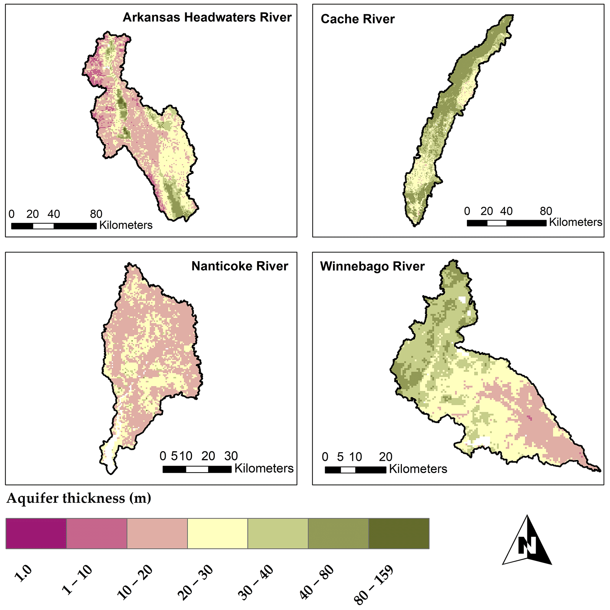
Figure 5 Schematic representation of aquifer thickness (m) maps for the four study watersheds of each grid cell.

As with the initial set-up of these models, the following features and limitations of the SWAT+gwflow modeling framework, as used in this study, should be noted:

1. The gwflow module only considers a single-layer heterogeneous unconfined aquifer in connection with the network of fields, channels and reservoirs.

2. Recharge from cultivated fields to the unconfined aquifer is explicitly simulated; however, recharge from non-field HRUs is not spatially explicit as the delineation of these HRUs is not provided in the NAM. Therefore, recharge for non-field areas is calculated using the average recharge rate for the 12-digit catchment.

3. The gwflow module does include an option to move water from the aquifer to the soil profile of the HRU if the water table rises above the base of the soil profile; using this process, shallow groundwater can be used as crop ET or discharged to nearby channels via soil lateral flow. However, due to the lack of spatial representation of non-field HRUs in the NAM, the groundwater → soil option is not possible. Therefore, shallow groundwater is allowed to rise to the ground surface, and, if groundwater head increases above the ground surface, the volume of water above the ground is routed as saturation excess flow to the nearest channel. We acknowledge this simplification but believe the methods to be adequate in regional-scale applications.

4. Groundwater fluxes along the boundary of the watershed are simulated using a boundary condition approach: the groundwater head in cells along the watershed boundary is assumed to be fixed at the initial value at the beginning of the simulation. If the cell head value is higher than adjacent head values, then groundwater inflow is simulated; if it is lower, then groundwater outflow is simulated. These fluxes are not calibrated per se; this is done indirectly as groundwater head values within the watershed are targets in model calibration.

2.2 SA–UA–PE methods for the SWAT+ models

In this section, we describe the application of SA, UA and PE tools to the watershed models constructed in Sect. 2.1. The general application of these tools to SWAT+gwflow is summarized in the schematic of Fig. 6. In this study, we demonstrate two possible operations: (1) PE with PEST followed by SA with the Morris method to identify system parameters that control streamflow and groundwater head for each watershed and (2) PE and UA with iES to provide prior and posterior ensembles of parameters and system responses (streamflow). The next sections describe the individual tools and how they are applied to the four watersheds.

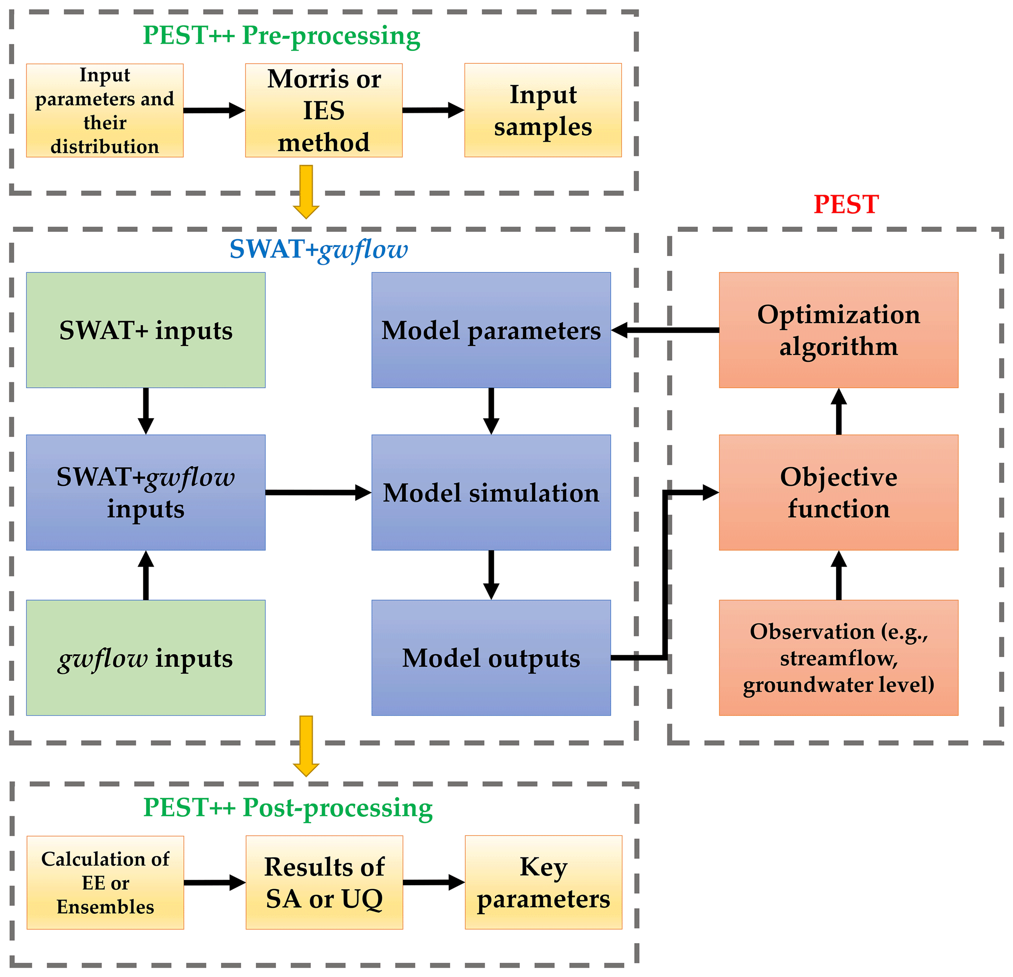
Figure 6 Schematic of PEST automatic calibration, sensitivity analysis and uncertainty analysis (iES) applied to the SWAT+gwflow models.

2.2.1 Method 1: Parameter ESTimation Tool (PEST) followed by sensitivity analysis

The SWAT+gwflow models are constructed based on a daily time step with a 2-year warm-up period (2000–2001) for the calibration period of 2002–2008 and validation period of 2009–2015. SWAT+gwflow models are first calibrated and tested using PEST (Doherty, 2020), a nonlinear, model-independent parameter estimator. PEST uses a local optimization technique that utilizes the Gauss–Marquardt–Levenberg algorithm (Doherty, 2004) to minimize the user-defined objective function (e.g., minimization of root mean squares between simulated and observed values). PEST has been broadly employed for sensitivity analysis, uncertainty quantification and model calibration for water quality and hydrologic models (e.g., Rode et al., 2007; Bahremand and De Smedt, 2010; Jiang et al., 2014).

In this study, we use all available monthly streamflow from USGS stream gage stations and average annual groundwater head from USGS monitoring wells in the objective function (OF). There are 1, 2, 3 and 4 stream gaging sites for the Winnebago, Nanticoke, Cache, and Arkansas Headwaters watersheds, respectively, and 7, 26, 92 and 3 monitoring wells (Fig. 2). The contributions of each of these sites to the composite OF were adjusted by manipulating the weights applied to the residuals to ensure that each site is of similar magnitude and significance in determining the optimal parameter values. Local optimization criterion (LOC) can be described as the weighted sum of the OF. The objective function is computed as the squared sum of weighted residuals. LOC and OF can be expressed as follows:

$$\begin{array}{}\text{(2)}& {\displaystyle }& {\displaystyle }\mathrm{OF}=\sum _{j=\mathrm{1}}^n{\left[x_{j,\mathrm{obs}}-x_{j,\mathrm{sim}}\right]}^{\mathrm{2}},\text{(3)}& {\displaystyle }& {\displaystyle }\mathrm{LOC}=\sum _{i=\mathrm{1}}^m{\mathit{\omega }}_i{\mathrm{OF}}_i,\end{array}$$

where n is the total number of the measured or simulated streamflow or groundwater monitoring wells, m is the total number of the observation groups of the observed streamflow from the gaging stations and groundwater monitoring wells, and ω is the weight of the related objective function.

The monthly simulated streamflow of the SWAT+gwflow models of the four study watersheds is evaluated using the determination coefficient (R²), Nash–Sutcliffe efficiency index (NSE), Kling–Gupta efficiency index (KGE) and percent of bias (PBIAS). The mean absolute error (MAE) is used to evaluate the performance of groundwater level at USGS monitoring wells. In our study, we set the maximum number of optimization iterations to 50. However, often, PEST converged after 22 iterations (1600 model calls) for Winnebago River, 13 iterations (674 model calls) and 36 iterations (2705 model calls) for Arkansas Headwaters, and 13 iterations (843 model calls) for Cache River.

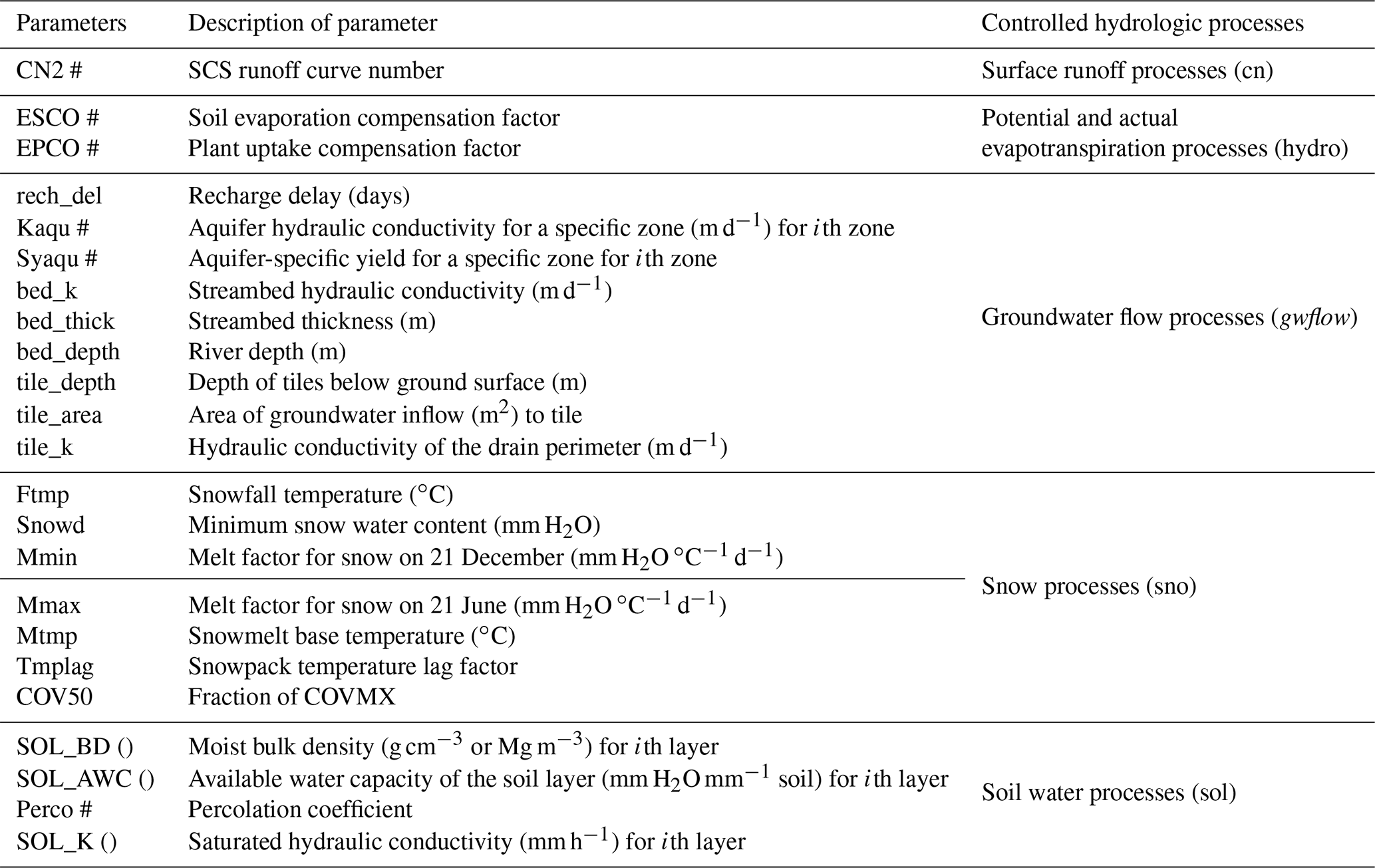
Based on SWAT model literature (e.g., Arnold et al., 2013; Koo et al., 2020), we selected 23 parameters to be modified by PEST (Table 3), focusing on surface runoff, evaporation, soil properties, groundwater processes, and snowmelt accumulation and melt processes. We set 2000–2001 as the warm-up period, 2002–2008 as the calibration period and 2009–2015 as the testing period. Therefore, in the initial PEST runs, we only use simulation periods of 2000–2008. Once PEST is finished for each watershed model, we then run each model for 2000–2015 to quantify criteria results (i.e., NSE, R², PBIAS, KGE and MAE).

Table 3 Description of hydrological fluxes of 23 selected parameters for the SWAT+gwflow model.

Once a parameter set was established using PEST, we applied the Morris screening method to each model to assess the impact of each parameter on streamflow and groundwater head. Morris screening (elementary-effects test) (Morris, 1991) is a qualitative global sensitivity analysis (GSA) technique that computes the relative sensitivity of model parameters by calculating the change in the model output given a change in the model parameter x_i value (i.e., elementary effect), with all other parameter values held constant. This procedure occurs over a range of parameter values, yielding a relationship between the parameter value and the model output. The following equation demonstrates the computation of a single elementary effect for the ith parameter:

$$\begin{array}{}\text{(4)}& {\mathrm{EE}}_i={\displaystyle \frac{f\left(x_{\mathrm{1}},\mathrm{\dots },x_i+{\mathrm{\Delta }}_i,\mathrm{\dots },x_p\right)-f\left(x\right)}{{\mathrm{\Delta }}_i}},\end{array}$$

where EE_i is the elementary-effect value of the ith model parameter; f represents the model; x₁, …, x_i is the model parameter value; and Δ represents the change. Within this method, the mean μ and standard deviation σ of all EE_i for a parameter are often used to assess the sensitivity or significance of parameters. To prevent the canceling of positive and negative values of EE_i, Campolongo et al. (2007) proposed using the absolute value of EE_i, yielding the mean μ^*. Therefore, μ^* and σ can be calculated as follows for a given parameter x_i:

$$\begin{array}{}\text{(5)}& {\displaystyle }& {\displaystyle }{\mathit{\mu }}_i^{*}={\displaystyle \frac{\mathrm{1}}{n}}\sum _{j=\mathrm{1}}^n\left|{\mathrm{EE}}_i\left(j\right)\right|,\text{(6)}& {\displaystyle }& {\displaystyle }{\mathit{\sigma }}_i=\sqrt{{\displaystyle \frac{\mathrm{1}}{n-\mathrm{1}}}\sum _{j=\mathrm{1}}^n{\left[{\mathrm{EE}}_i\left(j\right)-{\displaystyle \frac{\mathrm{1}}{n}}\sum _{j=\mathrm{1}}^n{\mathrm{EE}}_i\left(j\right)\right]}^{\mathrm{2}}},\end{array}$$

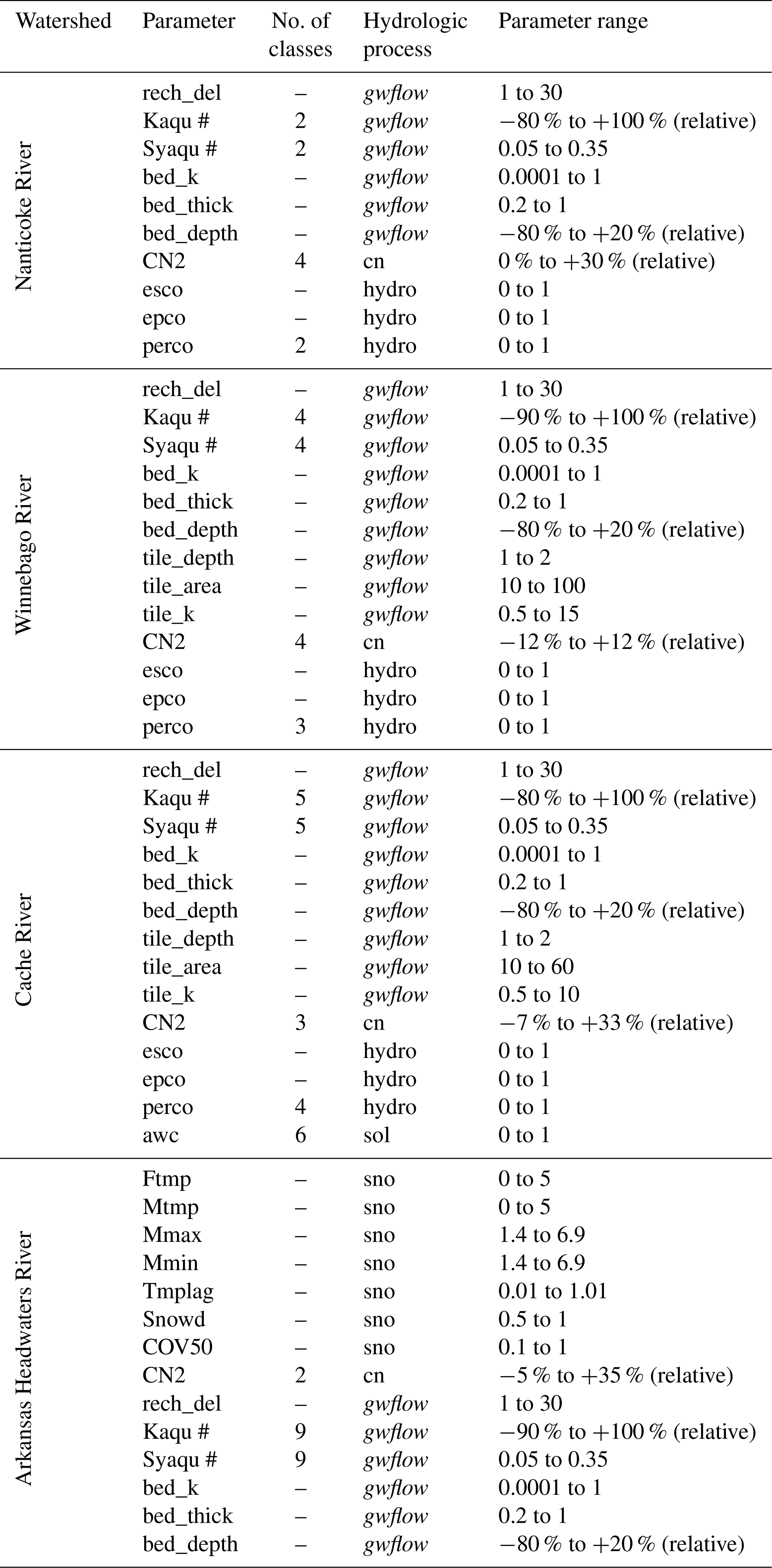
where n is the number of EE_i computations. The μ^* for the model parameters are then ranked to determine the parameters that have the strongest influence on model output. In this study, we implemented the Morris method using the software tool pestpp-sen (White et al., 2020), a variation of PEST. Table 4 lists parameters and their ranges for the four study watersheds. The number of classes (column 3) refers to the number of unique zones or categories for each parameter. For example, for Winnebago River, there are four aquifer zones, each with a different value of K and S_y.

Table 4 Selected parameters and ranges for the sensitivity and uncertainty analysis for the SWAT+gwflow model.

PEST is a powerful inverse modeling tool that can handle many parameters, needs linearity and a stable model, and requires several methods for parameter adjustment. However, determining the minimum of the objective function is restricted if there is a large amount of data error, if the model does not represent the data well, and if there is a high degree of correlation between the parameters.

2.2.2 Method 2: iterative ensemble smoother (iES) for parameter estimation and UA

In a second method, we use an iES (Chen and Oliver, 2013) to establish prior and posterior uncertainty estimates of model parameters within the pestpp-ies (White, 2018) framework that uses the PEST model interface. The iES is based on the original ensemble Kalman filter (EnKF) (Evensen, 1994), a data assimilation algorithm that updates state variables through assimilation of measured data into model results based on correlations between the state variables and the measurement data. For model parameters that have a strong influence on model results, the parameter values can also be updated through this data assimilation. Updates to state variables and parameters occur in a sequence of update steps. The EnKF was implemented in a smoother scheme, the ensemble smoother (ES) (Van Leeuwen and Evensen, 1996), in which all past states and parameters are updated in a single update step using all past measurement data. Chen and Oliver (2013) modified the ES to perform iteratively using the Gauss–Levenberg–Marquardt (GLM) algorithm, resulting in a significant decrease in computational burden for models with many parameters.

The iES method starts with an initial ensemble of values for each parameter (i.e., a prior ensemble). An estimation in relation to a Jacobian matrix of parameter sensitivities is computed based on the relationships between model parameters and model output using a range of parameter values based on the prior parameter ensemble (Chen and Oliver, 2013). The contents of the Jacobian matrix are then used to update the ensemble of each model parameter by seeking to minimize model residuals using the GLM algorithm. The result of the process is a posterior ensemble of model parameters that are optimally consistent with measured data. Table 4 lists parameters and their ranges used for iES application to the four study watersheds with three iterations of the data assimilation algorithm (250 model runs) in pestpp-ies. In general, the data assimilation approach assumes prior and posterior multivariate Gaussian parameter distributions.

3 Results and discussion

We first present hydrologic results for each of the four study watersheds through application of PEST, followed by the results of the Morris sensitivity analysis and the iES application.

3.1 Hydrologic state variables and fluxes

3.1.1 Streamflow and general water balance

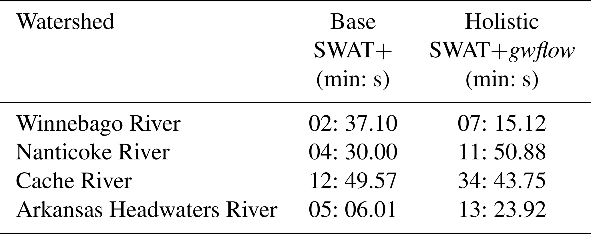
The comparison between observed and simulated monthly streamflow at 10 locations showed a good model performance based on NSE, R², PBIAS and KGE, as presented in Fig. 7 and Table 5, which shows the hydrograph of observed and simulated streamflow at four selected gages. By utilizing a desktop computer, an Intel^® Core^TM i7-10700 CPU @ 2.90 GHz with 64 GB RAM, simulation times for a whole period of simulation (2000–2015) for the four watersheds with SWAT+ and SWAT+gwflow are presented in Table 6, including the ranges 3–13 min for base SWAT+ and 7–35 min for SWAT+gwflow. These fast computation times greatly facilitate calibration, sensitivity analysis and uncertainty analysis for our regional-scale hydrologic models. Other physically based holistic hydrologic models could be used (e.g., HydroGeoSphere, Parflow, mHM), but the required heterogeneous parameters and long computation times are often prohibitive for the hundreds and thousands of simulations runs that are required for the sensitivity analysis and uncertainty analysis conducted in this study.

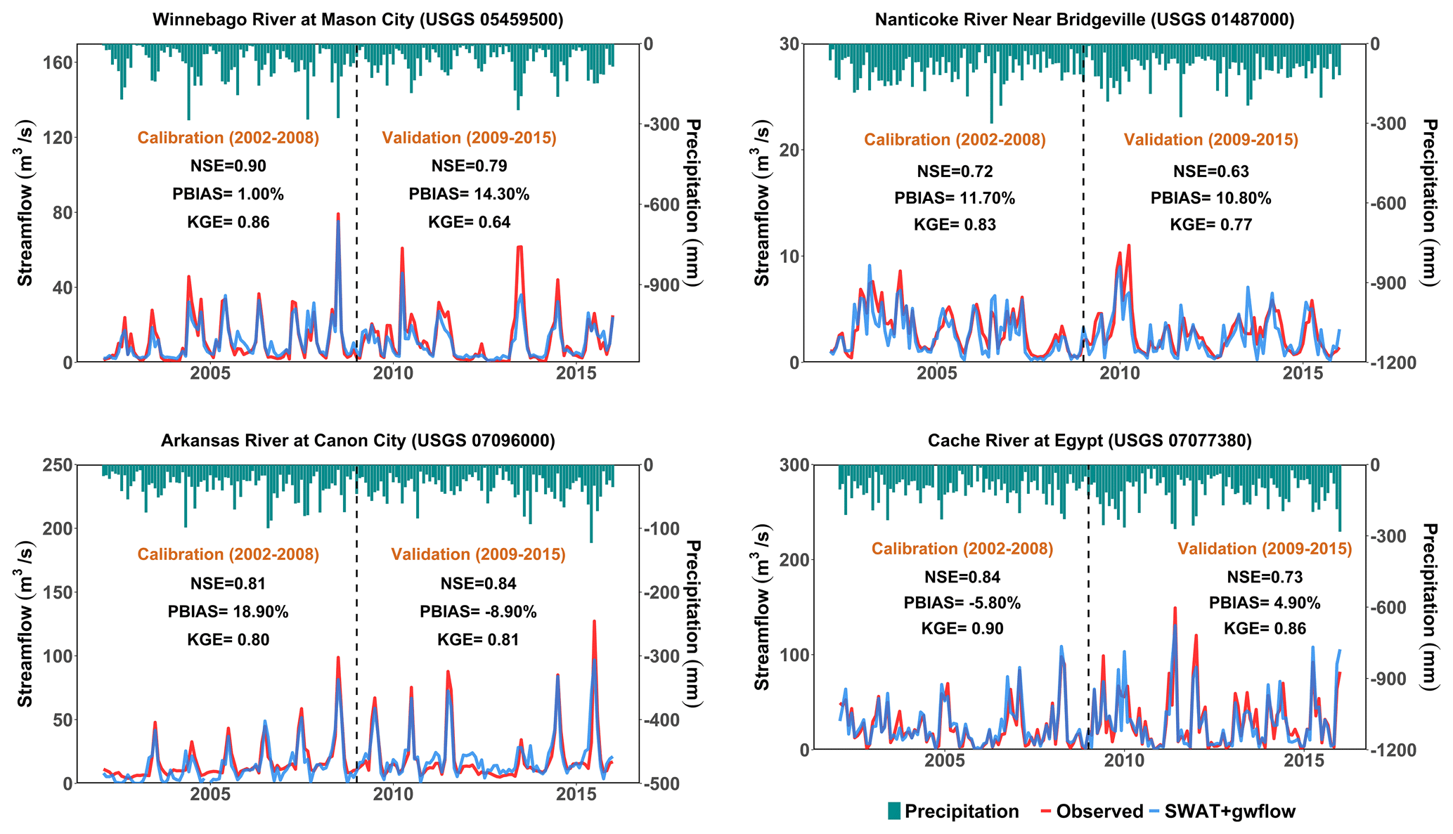
Figure 7 Measured and simulated monthly streamflow for SWAT+gwflow models for four selected river gage stations within the four study watersheds. Statistical model performances (NSE, PBIAS and KGE) are presented for each gage location.

Table 5 Monthly discharge statistical performance for the SWAT+gwflow simulation.

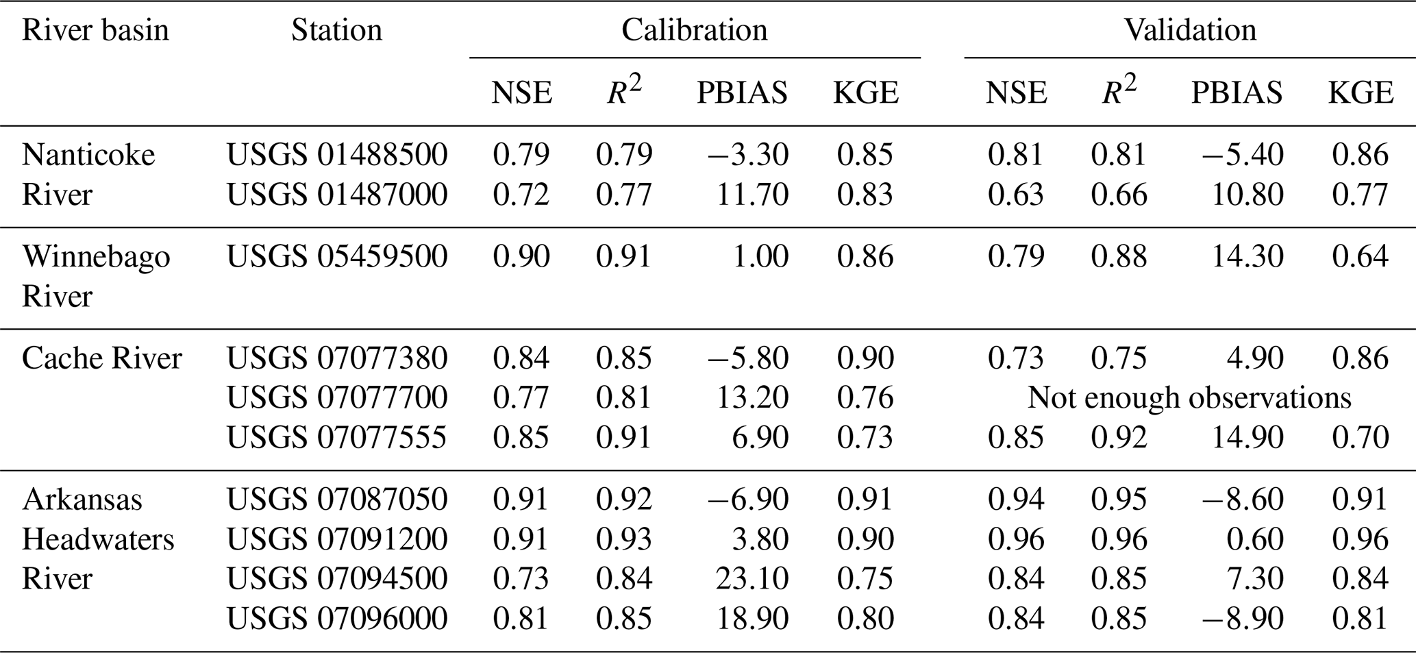
Table 6 Model run times for simulation period of 2000–2015 for four study areas using standalone SWAT+ and holistic SWAT+gwflow.

3.1.2 General watershed fluxes

Table 7 displays the annual average hydrologic fluxes for the four study watersheds. Catchment key inflows include groundwater inflow from adjacent aquifer along the catchment boundary and precipitation. Catchment key outputs comprise soil lateral flow, surface runoff, evapotranspiration ET, tile drainage flow, saturation excess flow and stream seepage.

Table 7 Mean annual hydrologic flow processes (mm) for four study watersheds with main flux fraction.

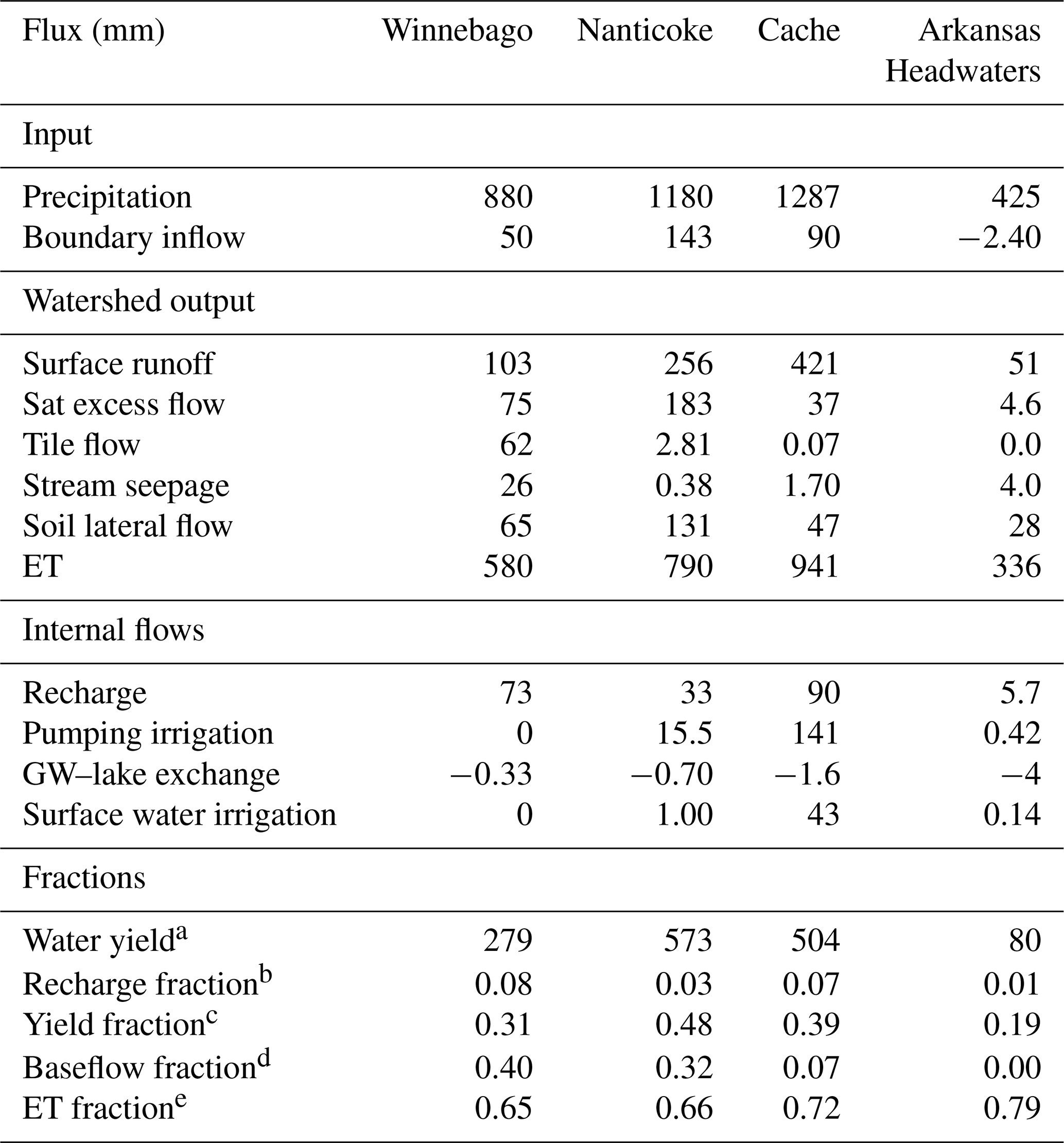
^a Water yield = surface runoff + lateral flow − stream seepage + saturation excess flow + tile flow. ^b Recharge$/$precipitation. ^c Water yield$/$precipitation. ^d Net groundwater inflow to streams (sat excess flow + tile flow − stream seepage)$/$water yield. ^e ET$/$precipitation.

The internal flows to the watershed include surface water irrigation (calculated by SWAT+), pumping irrigation (computed by gwflow), recharge (computed by gwflow), and groundwater–reservoir and groundwater–lake exchange (calculated by gwflow). Table 7 also reveals key hydrologic fractions and average annual water yield. Cache has an annual value of 141 mm for groundwater pumping for irrigation. Notably, Winnebago has the highest flow of tile drain (62 mm), and Nanticoke River demonstrates high fluxes of groundwater to the stream network with saturation excess flow of (183 mm).

Arkansas Headwaters and Cache have small net groundwater discharge to stream (+ 37 sat excess flow − 1.7 mm seepage = +35.3 mm for Cache) and (−4 mm seepage + 4.6 sat excess flow = +0.6 mm for Arkansas Headwaters) owing to deeper groundwater levels in comparison to stream stage. The baseflow contribution is moderate (>0.30) for Winnebago and Nanticoke rivers and low (<0.20) for the other watersheds. The yield fraction, i.e., the ratio of water yield in the streams to precipitation, ranges from 0.19 (Arkansas Headwaters) to 0.48 (Nanticoke). The recharge fraction ranges from 0.01 (Arkansas Headwaters) to 0.08 (Winnebago), with recharge fluxes for several of the watersheds being similar in magnitude to soil lateral flow and surface runoff.

3.1.3 Monthly hydrologic fluxes

Figure 8 reveals monthly hydrologic flow processes for the period of 2002–2015 for each watershed. Plots on the left show results for the entire watershed system, whereas plots on the right show results for the aquifer system. Key watershed inflows are boundary inflow and precipitation, where watershed outflows are tile drainage, groundwater saturation excess flow, runoff, surface ET and lateral flow, which showed watershed seasonal fluxes for each basin. The Winnebago River is notable for its high flux rates of tile drainage outflow, groundwater exchange with reservoirs and lakes in the Arkansas Headwaters River, seasonal pattern of saturation excess flow (i.e., groundwater that reaches the river due to groundwater flooding) in the Nanticoke River, and groundwater pumping in the Cache River watershed, exhibiting the unique hydrologic characteristics of each watershed in relation to groundwater storage and flow.

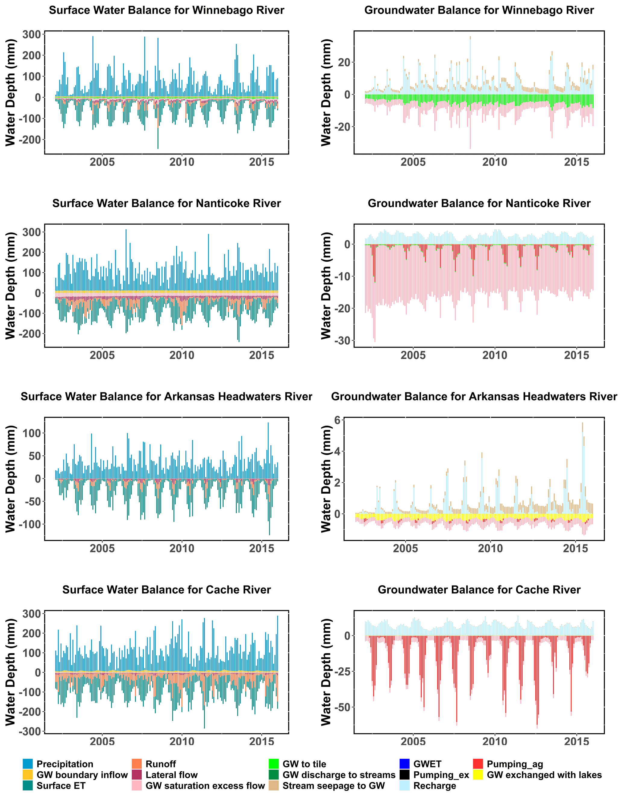
Figure 8 Monthly surface water fluxes (mm) (left panels) and groundwater fluxes (mm) (right panels) for the simulation period of 2002–2015 for the four study watersheds.

3.1.4 Groundwater head

Figure 9 contains the statistical performance based on mean absolute error (MAE) of annual groundwater level for four study watersheds for the period of 2000–2015. MAE results show an acceptable error (<1.5 m residual in groundwater level) between simulated and measured average annual groundwater head at each USGS monitoring well site. However, a few locations have higher error (2.5–3.6 m difference), although these residuals are small compared to the saturated thickness of the aquifer.

Figure 9 Maps showing statistical model performance based on mean absolute error (MAE) (m) for groundwater level for the simulation period of 2000–2015 in the study watersheds.

3.1.5 Spatial variation of groundwater fluxes

Figure 10 shows saturated-thickness maps (that is, vertical distance between bedrock and water table) for the final year of simulation (2015) for the study watersheds, with saturated thickness being similar in spatial pattern to the thickness of the unconfined aquifer (see Fig. 5) but differing due to spatial changes in groundwater head within each watershed.

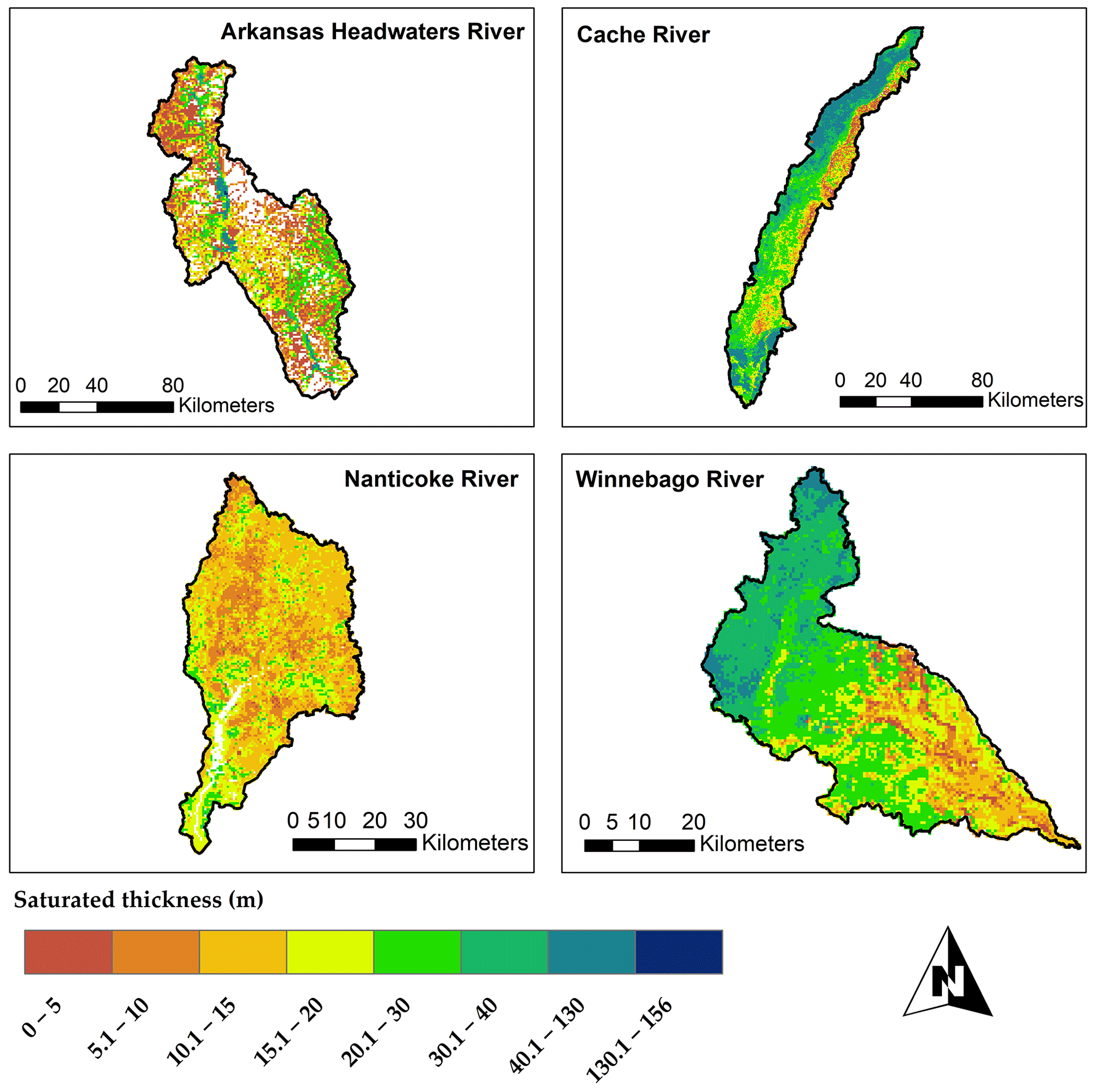
Figure 10 Maps of saturated thickness (m) in the four study watersheds.

Raster maps of average daily groundwater sink–source flow processes (Figs. 11–13) demonstrate zones of stress within the aquifer unit and regions of main inflows into the stream channel system. Spatial fluxes of recharge, groundwater–stream interaction (i.e., saturation excess flow) and groundwater pumping are presented as maps in Figs. 11–13, respectively. Saturation excess flow occurs where the water table is shallow. Groundwater pumping for irrigation is presented for Nanticoke and Cache since the other two watersheds do not experience groundwater pumping for irrigation. Cache has the highest pumping rates due to extensive irrigation practices in the region.

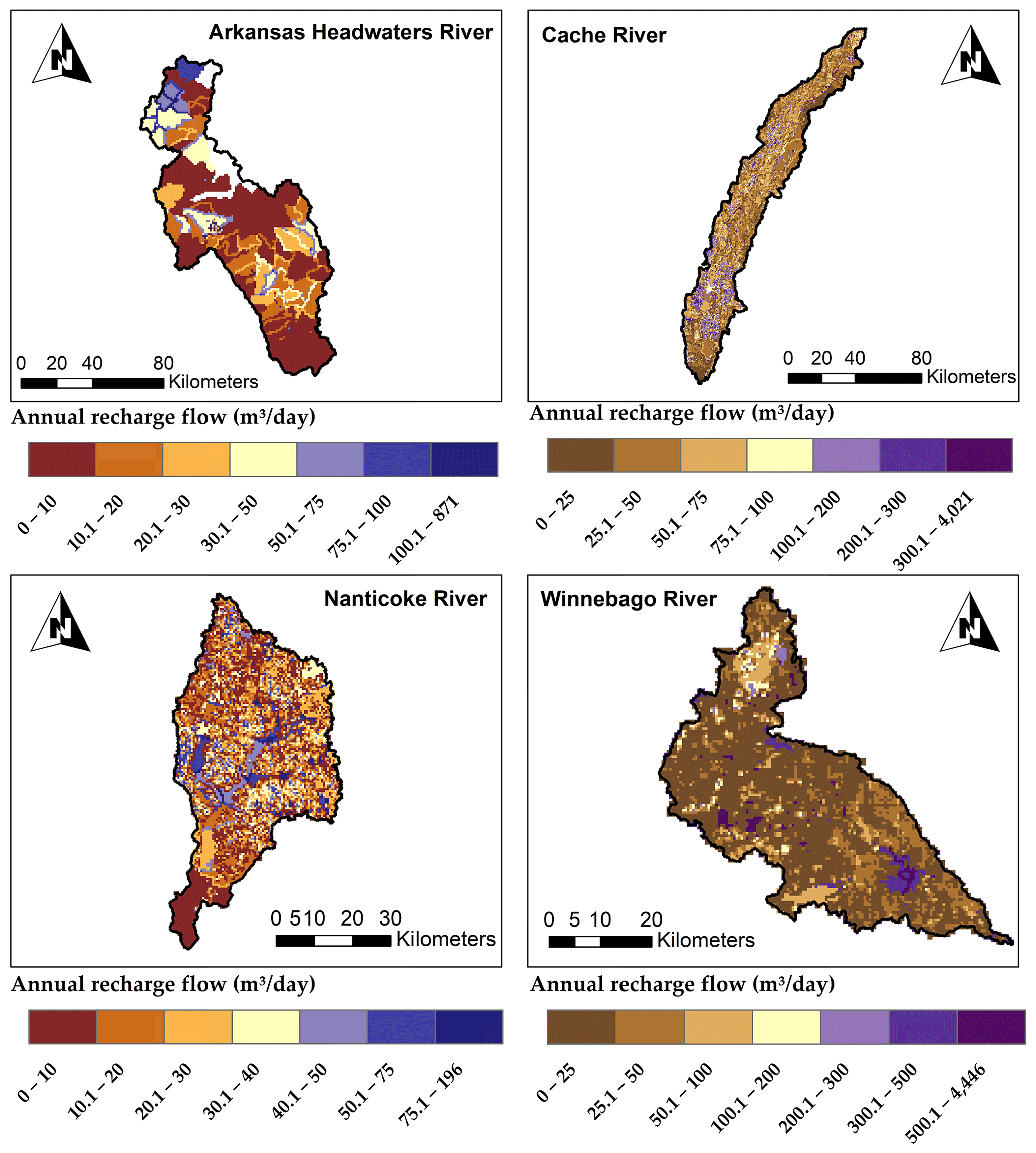
Figure 11 Maps of average annual recharge flow (m³ d⁻¹) for the period of 2000–2015 for each of the study watersheds for each grid.

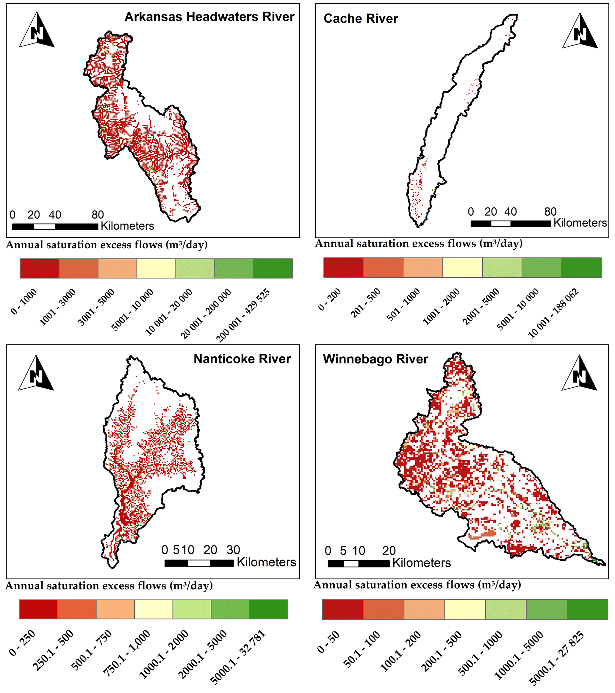
Figure 12 Maps of average annual saturation excess flow (m³ d⁻¹) for the period of 2000–2015 in each of the four study watersheds for each grid.

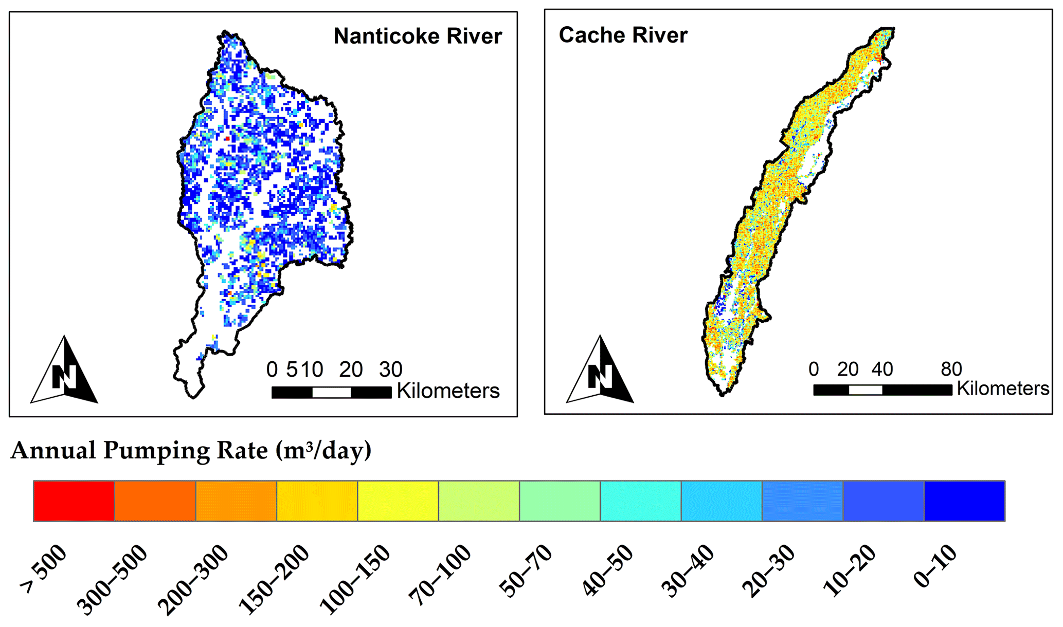
Figure 13 Maps of average annual groundwater pumping for irrigation (m³ d⁻¹) in the Cache and Nanticoke watersheds for each grid cell.

Within the SWAT+gwflow framework, stream seepage and groundwater saturation excess runoff constitute groundwater–stream interaction. Throughout the stream system, seepage to the aquifer occurs, with the highest rates typically being found along the major rivers because of the large head difference between the stream and the surrounding water table at those locations. High values of saturation excess runoff can be found in the vicinity of rivers and streams in areas of shallow groundwater levels.

3.2 Sensitivity analysis using the Morris screening method

The Morris results for parameter influence on streamflow (Fig. 14) show the most influential parameters for each study watershed:

1. For Winnebago, there is the percolation coefficient (Perco1), streambed thickness (bed_thick), hydraulic conductivity of the drain perimeter (tile_k) and streambed hydraulic conductivity (bed_k). These results indicate that streamflow is controlled principally by processes that affect tile drainage and stream–aquifer interactions. This is somewhat surprising as surface runoff is the dominant flux contributing to streamflow.

2. For Nanticoke, there is specific yield (syaqu2), hydraulic conductivity (kaqu2), streambed thickness (bed_thick) and streambed hydraulic conductivity (bed_k). These results indicate that groundwater properties and processes control streamflow, in agreement with the high baseflow fraction (0.32) of the watershed (Table 7).

3. For Arkansas Headwaters, there is the melt factor for snow on 21 June (Mmax), snowmelt base temperature (Mtmp), streambed thickness (bed_thick), snowpack temperature lag factor (Tmplag) and curve number (cn_frstgd). This is not surprising as the streamflow is dominated by springtime snowmelt patterns.

4. For Cache, there is the soil evaporation compensation factor (esco), percolation coefficient (Perco2), specific yield (syaqu4), streambed hydraulic conductivity (bed_k), curve number (rcsr_gd), available water capacity (awc3), thickness (bed_thick), plant uptake compensation factor (epco) and recharge delay (rech_del). Streamflow in this watershed is dominated by processes that affect surface runoff (421 mm in Table 7) and groundwater pumping (141 mm).

Morris results for the parameter influence on groundwater level (Fig. 15) show the most influential parameters for each study watershed:

1. For Winnebago, there is the streambed hydraulic conductivity (bed_k), indicating the strong influence of stream–aquifer interactions on groundwater head in the region.

2. For Nanticoke, there is the specific yield (syaqu2) and hydraulic conductivity (kaqu2).

3. For Arkansas Headwaters, there is the hydraulic conductivity (kaqu9) and specific yield (syaqu6).

4. For Cache, there is the soil evaporation compensation factor (esco), curve number (rcsr_gd) and available water capacity (awc3 and awc4), indicating the influence of land surface and soil processes on groundwater head due to their control on the volume of groundwater that is pumped from the aquifer.

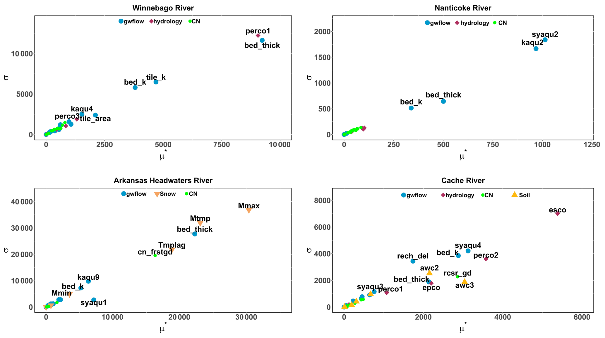
Figure 14 Parameter sensitivity analysis based on the Morris screening method for minimizing streamflow. Only the most sensitive parameters are labeled. σ reveals the degree of nonlinearity or factor interaction, and μ^* is the sensitivity measure. These sensitivity measures are based on elementary effects and are not related to the scale and magnitude of the input or output quantities; therefore, results show relative relation between parameters.

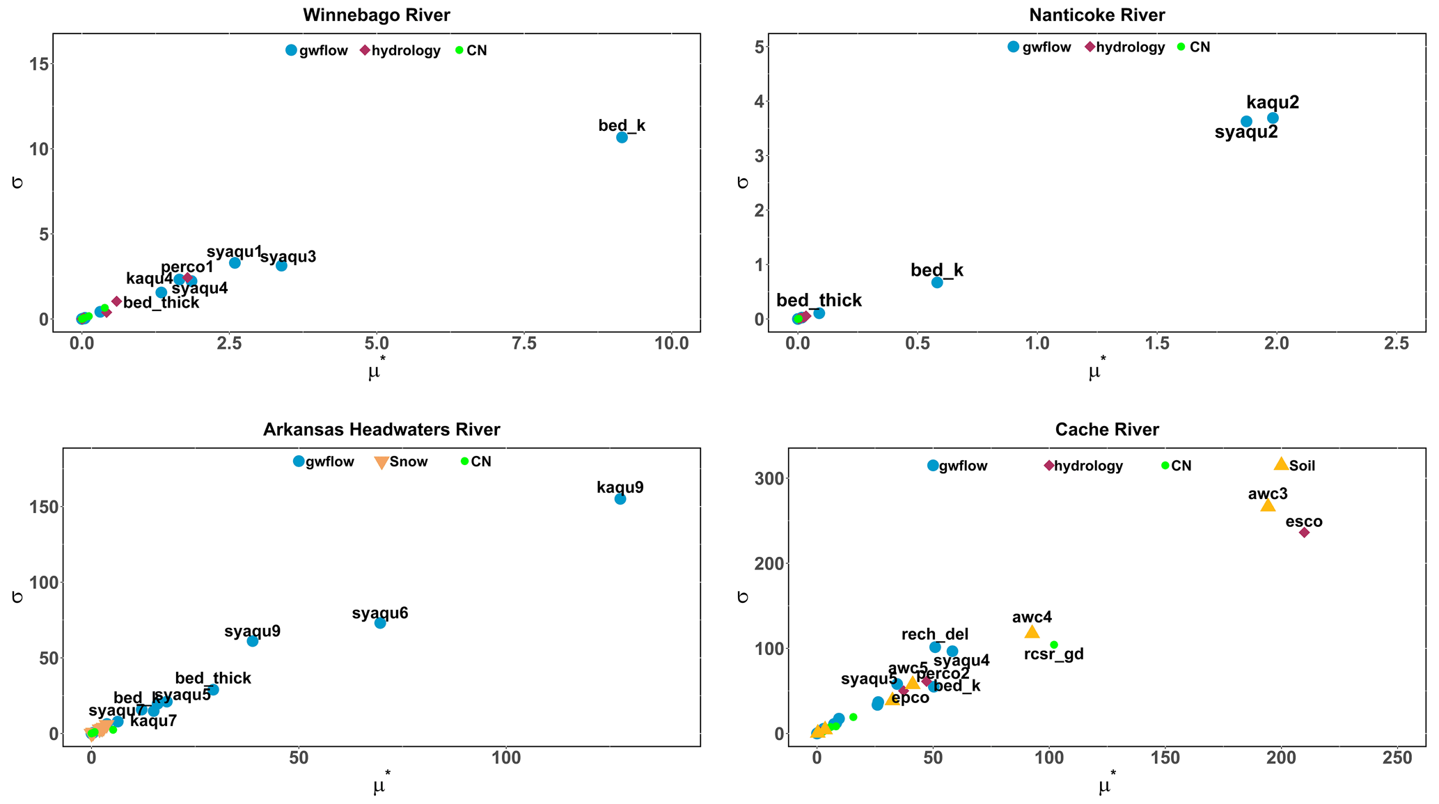
Figure 15 Parameter sensitivity analysis based on the Morris screening method for minimizing groundwater level. Only the most sensitive parameters are labeled. σ reveals the degree of nonlinearity or factor interaction, and μ^* is the sensitivity measure. These sensitivity measures are based on elementary effects and are not related to the scale and magnitude of the input or output quantities; therefore, results show relative relation between parameters.

The estimated time-varying parameter sensitivity calculated by the Morris method is represented in Fig. 16 for the most influential parameters in the four watersheds. These values are a combination of streambed parameters (bed_k), soil parameters (perc1, esco), snow parameters (Mmax, Mtmp) and aquifer parameters (syaqu2, kaqu2), depending on the watershed. The Nanticoke River model is dominated by aquifer parameters due to shallow groundwater levels and associated groundwater discharge to the stream network. The Arkansas River model is dominated by snow parameters due to mountainous terrain in the Rocky Mountains. These results indicate that these parameters have a seasonal fluctuation in their influence on streamflow due to the seasonal fluctuations and timing of groundwater levels, snowfall and crop growth.

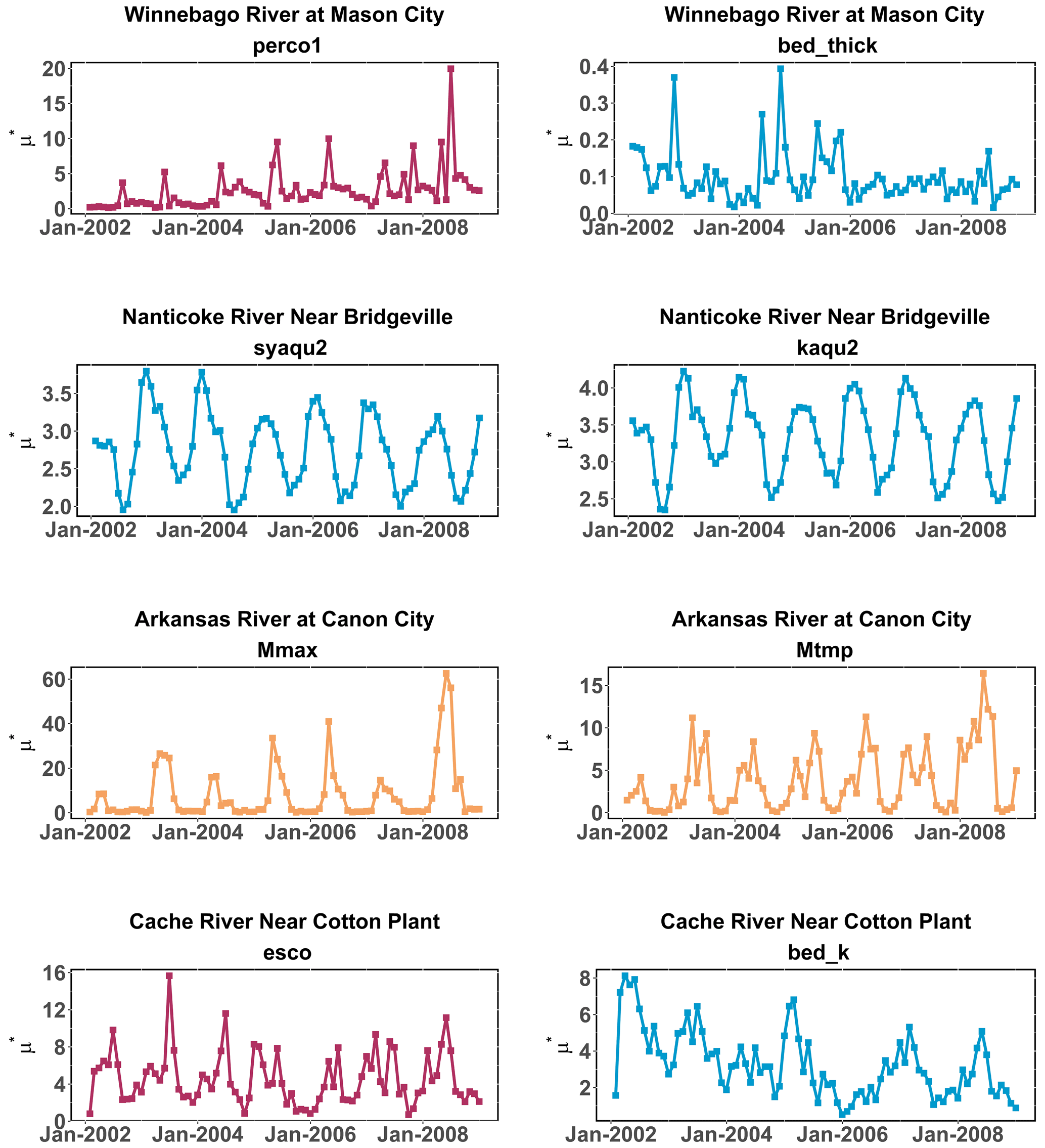
Figure 16 Estimated sensitivity that changes with time for the streamflow for the key influential parameters of the four study watersheds. The blue lines represent gwflow parameters, maroon lines are for hydrology parameters, and orange lines represent the snow parameters.

The strong influence of streambed parameters (streambed conductivity, streambed thickness) on system responses in each of the four study watersheds is expected due to the coupled surface–subsurface nature of the watersheds. Water exchange between channels and aquifers increases with increasing conductivity and decreasing thickness. Streambed parameters have a strong control on streamflow for each of the four watersheds, whereas they control groundwater head for only the Winnebago River watershed and the Nanticoke River watershed due to shallow groundwater levels in relation to ground surface and channel elevation. For streamflow, control is either in the direction of channel → aquifer (seepage) or aquifer → channel (discharge). For the Cache River watershed, extensive groundwater pumping (see Fig. 13) can lead to enhanced stream seepage (streamflow depletion) which, as noted by previous studies (Fox and Durnford, 2003; Fox, 2007), can be sensitive to streambed conductivity. In general, the importance of streambed parameters such as conductivity and thickness in the modeling of surface–groundwater (SW–GW) exchange fluxes has been noted extensively (Kalbus et al., 2009; Brunner et al., 2017; Partington et al., 2017), with many studies aiming to quantifying these parameters spatially (e.g., Fox, 2007; Crook et al., 2008; Wojnar et al., 2013; Shi and Wang, 2023).

3.3 Uncertainty analysis and parameter estimation using the iES

Figure 17 shows the observed and best estimated monthly streamflow with prior and posterior prediction uncertainty bands for the four study watersheds. The plots in the left column represent prior parameter ensembles (uncalibrated Monte Carlo results) with wide uncertainty bands. Meanwhile, the plots in the right column show the posterior ensemble that effectively reduces the uncertainty band. For example, in Arkansas Headwaters, the prior ensemble uncertainty band was shifted to the left of the measured streamflow, owing to an incorrect characterization of snowmelt timing and magnitude. However, the posterior ensemble uncertainty band is much narrower and fits the timing and magnitude of the measured streamflow.

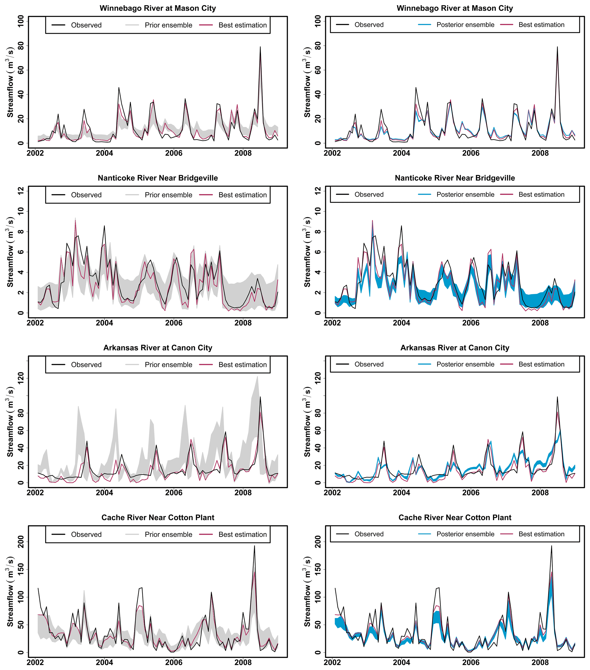
Figure 17 Prior (left panels) and posterior (right panels) prediction uncertainty bounds for streamflow estimation for SWAT+gwflow for four study watersheds.

Figure 18 demonstrates the effect of data assimilation on the parameters more quantitatively, which compares the histogram of prior parameter ensembles (gray) with the histogram of posterior parameter ensembles (blue) for nine of the most influential parameters in the four study watersheds. The posterior distribution of parameters is narrower than the prior distribution, which helps in the estimation of model parameters. The range parameters for curve number–Cache River (Fig. 18h) and specific yield–Nanticoke River (Fig. 18c) indicate the largest influence of data assimilation. Short correlation ranges have been reduced from the posterior.

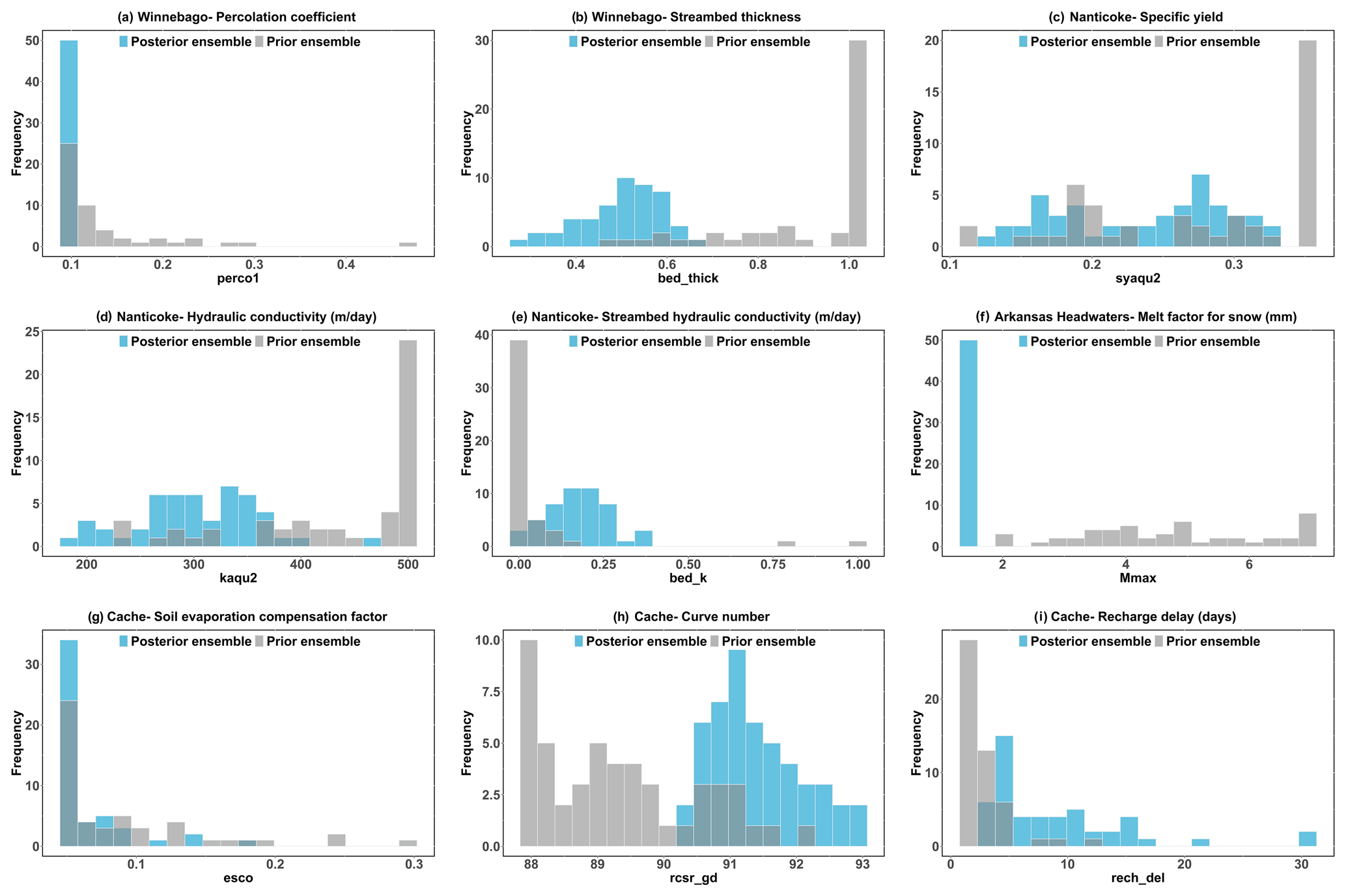
Figure 18 Histogram for prior and posterior for significant parameters for four study watersheds.

Figure 19 shows the influence of data assimilation on the average annual water balance more quantitatively, which compares the histogram of prior ensembles (gray) with the histogram of posterior ensembles (blue) for the eight most important water balance components in the four study watersheds. The posterior distribution of parameters is narrower than the prior distribution, which helps in the estimation of the water balance component.

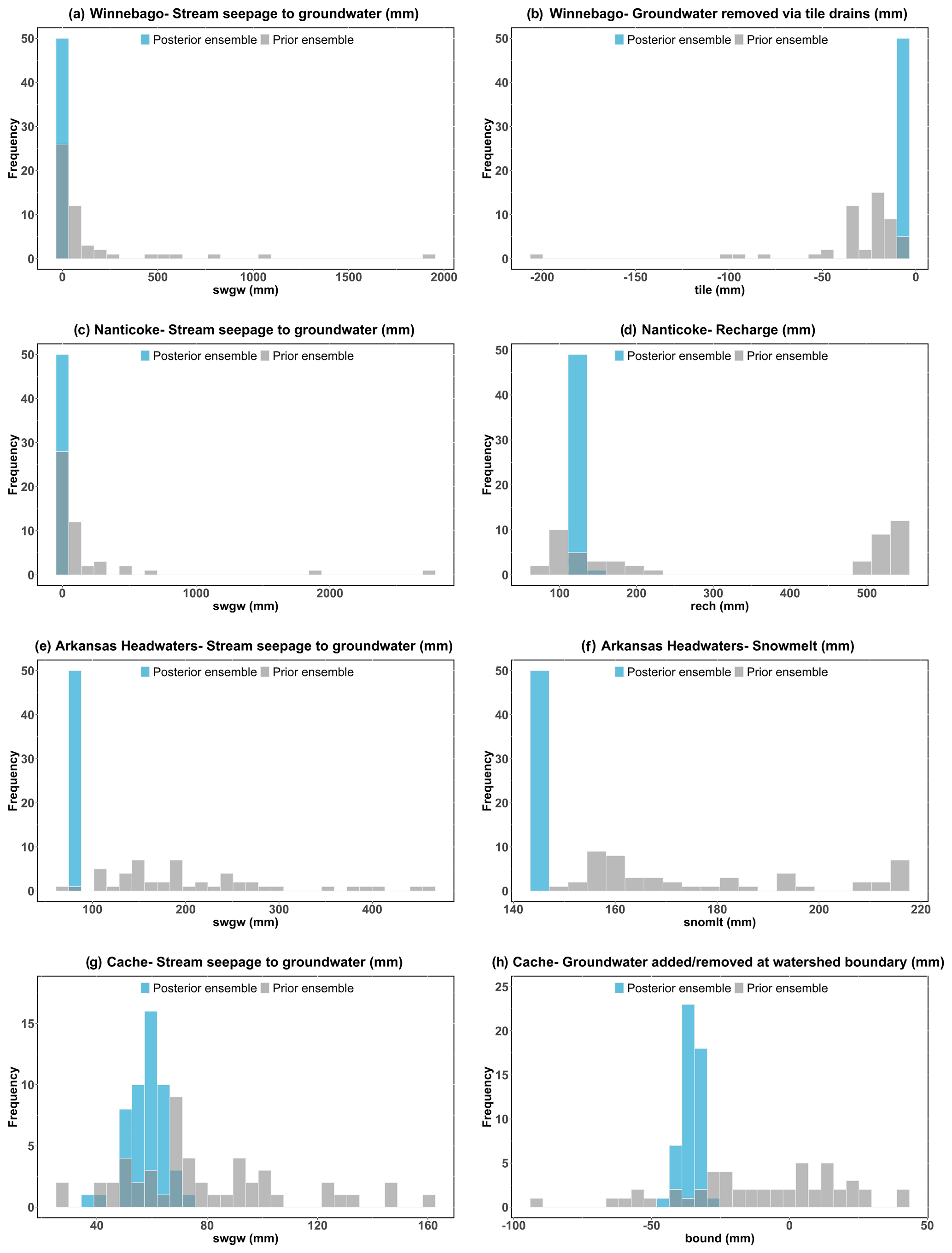
Figure 19 Histogram for prior and posterior average annual water balance components (significant components) for four study watersheds.

In general, the application of the iES can provide ensembles of posterior parameter sets that, when used in the model, provide simulation results that are in close comparison with measured data and, due to the use of ensembles, includes uncertainty in results. When used for scenario analysis and decision making, these models can employ the posterior ensembles of parameters to propagate uncertainty into model results, therefore serving effectively in the role of decision support.

In general, ensemble-based data assimilation naturally accommodates parameter correlation, both in the prior parameter distribution (as expressed in the prior parameter covariance matrix) and in correlations between parameters that give correlated responses to historic observations. The former is addressed simply by providing the requisite covariance matrix or by generating a prior parameter ensemble that is imbued with appropriate parameter relations. The latter correlations, those typically referred to as being non-unique, are handled algorithmically through the truncated singular value decomposition (SVD) solution as a mechanism to stabilize the inverse problem, as well as implicitly through the use of an ensemble that is naturally rank deficient (in that it does not fully occupy the range space of the parameter space). The rank-deficient ensemble used to approximate the Jacobian matrix only occupies the dominant singular components of the full Jacobian – these dominant singular components are a subspace that includes the parameter combinations that represent parameters that are non-unique with respect to the historical observations. It is worth noting that one of the strengths of an ensemble-based approach to history matching is that the posterior parameter spans this non-uniqueness. Results for stand-alone SWAT+ models, i.e., models without the gwflow module included, are provided in the Supplement.

4 Summary and conclusions

In this article, we present two methods to include sensitivity analysis, uncertainty analysis and parameter optimization into coupled surface–subsurface hydrologic models using the SWAT+ model as an example. The method utilizes the gwflow module, which is a spatially distributed, physically based groundwater flow module coupled to the SWAT+ model, which utilizes aquifer control volumes (i.e., grid cells) to compute daily water balance in an unconfined aquifer. We present our technique for four different US watersheds: Winnebago River, Nanticoke River, Cache River and Arkansas Headwaters. These watersheds were selected on account of their respective unique hydrologic features: an extensive network of tile drain (Winnebago), shallow groundwater (Nanticoke), snowmelt dominance (Arkansas Headwaters) and extensive groundwater pumping for irrigation. The SWAT+gwflow models are calibrated based on the monthly streamflow and annual groundwater level for the period of 2000–2008 with a 2-year warm-up period, validated for a period of 2009–2015. The parameter estimation software PEST and PEST$++$ are used for the calibration, sensitivity analysis and uncertainty analysis of hydrologic models. Additionally, watershed water balance fluxes are evaluated for the stability of models. All watershed models showed good statistical performance of streamflow simulation (10 river gage locations) and groundwater level results (128 monitoring wells); however, a few wells exhibited high values of mean absolute error results. Model outputs comprised saturated thickness (spatial maps), raster maps of groundwater flow processes (saturation excess flow, stream seepage, pumping, recharge), which can be utilized to validate the model and recognize areas that need further parameter estimation; groundwater head (time series and spatial maps of observation locations); and stream discharge. By combining average annual water balance fluxes, groundwater head and streamflow data, hydrologic flow processes can be restricted to realistic ranges. Increased fidelity in process representation allows these modeling tools to be utilized for the assessment of water resources under different land use and climate scenarios over a wide range of hydrologic conditions.

GSA using the Morris screening technique was applied to SWAT+gwflow models of study watersheds to assess the governing system factors in relation to surface runoff and groundwater fluxes. The pestpp-sen tool within the PEST$++$ environment is utilized to generate parameter values, update model files for SWAT+gwflow models, run the model simulations and compute sensitivity indices for the Morris method. The sensitivity of 23 parameters (including surface runoff fluxes, actual and potential evapotranspiration fluxes, groundwater flow fluxes, snow fluxes, and soil water fluxes) were investigated based on two model responses: minimizing monthly streamflow and minimizing the mean absolute error (MAE) of annual groundwater head data.

The iES method was used for the model input uncertainty for the prior (uncalibrated results) and posterior ensembles, thus resulting in better uncertainty prediction that will improve the utilization of hydrologic models in decision making. This technique is implemented using the pestpp-ies tool within the PEST$++$ environment.

From the results, we conclude the following:

1. Winnebago River (extensive presence of tile drainage). Groundwater-flow-related parameters and soil water parameters significantly affect streamflow and groundwater heads, especially percolation coefficient, streambed thickness, hydraulic conductivity of the drain perimeter and streambed hydraulic conductivity.

2. Nanticoke River (intensive surface–groundwater interaction). Groundwater-flow-related parameters notably influence streamflow and groundwater heads, specifically specific yield, hydraulic conductivity, streambed thickness and streambed hydraulic conductivity.

3. Arkansas Headwaters River (snowmelt-dominant basin). Snow processes and surface-runoff-flow-related parameters extensively affect streamflow, while groundwater flow parameters significantly influence groundwater heads. Snow parameters include the melt factor for snow on 21 June, snowmelt base temperature, streambed thickness, snowpack temperature lag factor and curve number for surface runoff processes. Groundwater flow parameters hydraulic conductivity and specific yield.

4. Cache River (extensive groundwater pumping for irrigation). Soil-water-related parameters significantly affect streamflow, including soil evaporation compensation factor and percolation coefficient. Meanwhile, groundwater flow and surface runoff have parameters with relatively less influence on stream discharge. For groundwater head, soil-water-related parameters pointedly affect streamflow comprising available water capacity and the soil evaporation compensation factor.

5. The iES method. This represents prior parameter ensembles (uncalibrated Monte Carlo results) with wide uncertainty bands, and the posterior ensemble effectively reduces the uncertainty band. This technique can give best-estimation parameter ranges, water balance components, and simulated streamflow and groundwater heads.

While these SA–UA–PO methods have been demonstrated here for the SWAT+gwflow model, they can be applied generally to other coupled surface–subsurface models or even stand-alone watershed models such as SWAT or SWAT+.