Hydrological objective functions and ensemble averaging with the Wasserstein distance

When working with hydrological data, the ability to quantify the similarity of different datasets is useful. The choice of how to make this quantification has a direct influence on the results, with different measures of similarity emphasising particular sources of error (for example, errors in amplitude as opposed to displacements in time and/or space). The Wasserstein distance considers the similarity of mass distributions through a transport lens. In a hydrological context, it measures the “effort” required to rearrange one distribution of water into the other. While being more broadly applicable, particular interest is paid to hydrographs in this work. The Wasserstein distance is adapted for working with hydrographs in two different ways and tested in a calibration and “averaging” of a hydrograph context. This alternative definition of fit is shown to be successful in accounting for timing errors due to imprecise rainfall measurements. The averaging of an ensemble of hydrographs is shown to be suitable when differences among the members are in peak shape and timing but not in total peak volume, where the traditional mean works well.

1 Introduction

1.1 Motivation

A fundamental aspect of hydrology is understanding the distribution and movement of water through the Earth system. It is therefore necessary to quantify the similarity of a pair of spatial (e.g. precipitation fields) or temporal (e.g. hydrographs) distributions of water. The goal of this quantification may simply be to gauge the semblance of the distributions. In other more complex cases, it may act as an objective function for parameter estimation, model calibration, or data assimilation, where the goal is to minimise the discrepancy between a model output and observed data. Again still, we may be interested in the “average” distribution of water among an ensemble. Each of these varied tasks is unified in the requirement of some measure of similarity between pairs of distributions, with the characteristics of this choice important for the quality of the result.

Such a quantification varies in nomenclature according to discipline and purpose, but some common terms are “objective”, “response”, or “misfit function”. While it is abundantly clear that there is a great need for comparative measures in hydrology, there remains ambiguity in selecting that which best quantifies discrepancy for any given application. In this selection process, we are led back to the more fundamental query: what is a good “fit”? The misfit function that we use must be intrinsically linked with what we perceive to be a “good fit” for the application and purpose at hand.

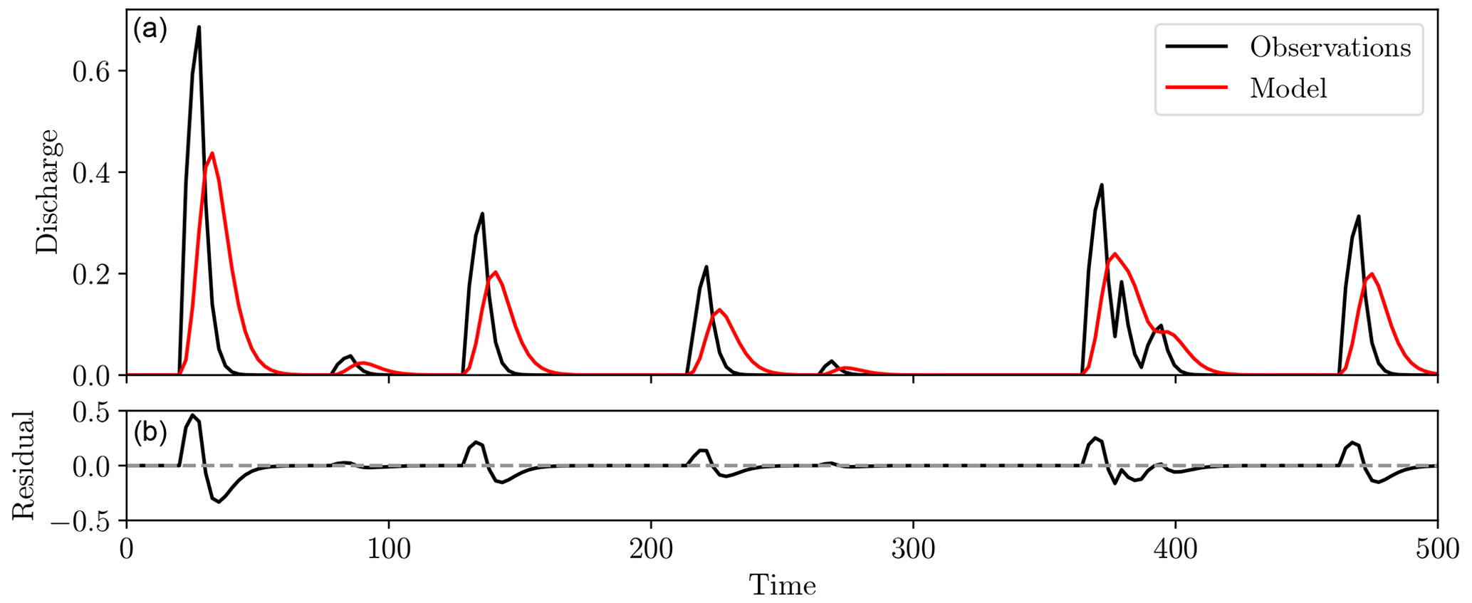
Figure 1 Two hydrographs (a, red and black) and the point-wise residuals between them (b). Both timing and amplitude differences are observed, but these are combined into a single amplitude error to give large residuals, even though the human eye might perceive these two distributions as being quite close.

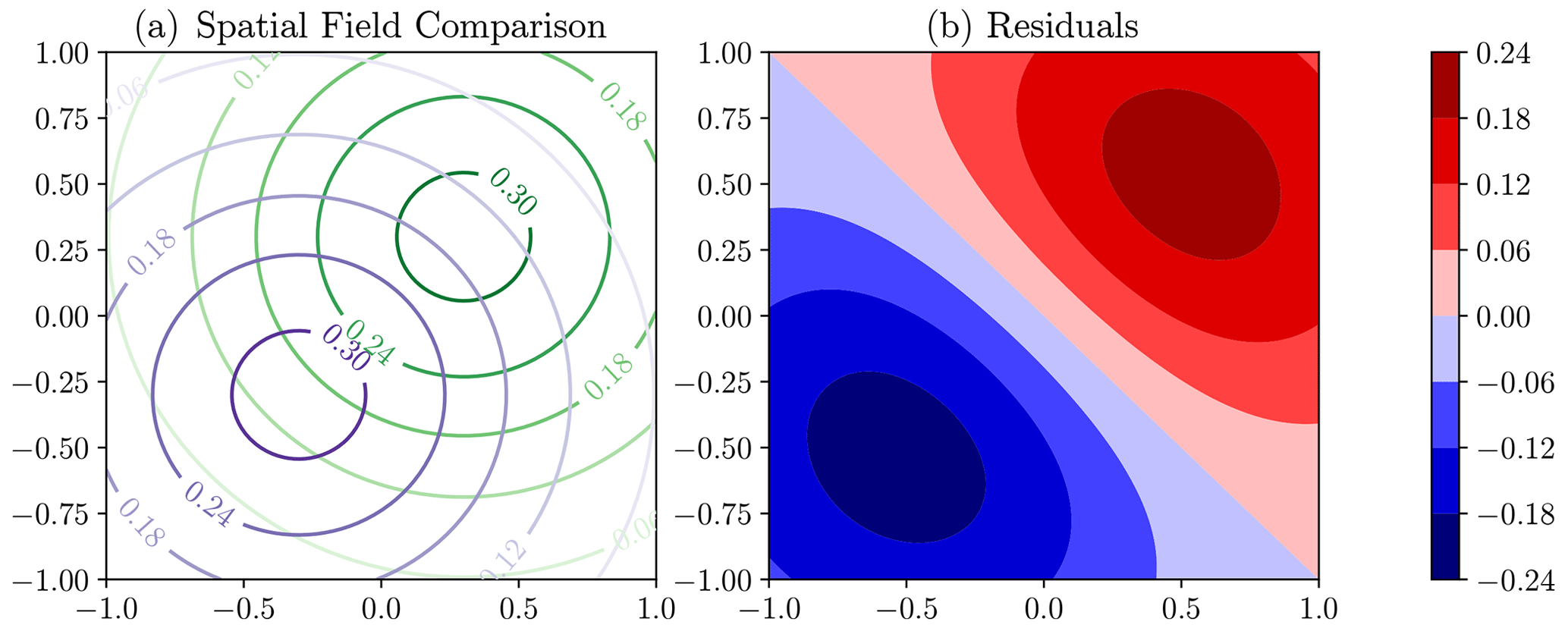
Figure 2 Synthetic example of the comparison of modelled (purple) and observed (green) spatial fields in panel (a). Panel (b) shows the residuals (green field minus purple field), which display the double-penalty effect as the error is in displacement rather than amplitude.

A commonly used metric for comparing both hydrographs and spatial fields is the root mean square error (RMSE), given by Eq. (1), where f and g are the functions under comparison and have known values at the N points x_i.

$$\begin{array}{}\text{(1)}& \mathrm{RMSE}=\sqrt{{\displaystyle \frac{\sum _{i=\mathrm{1}}^N{\left[f\left(x_i\right)-g\left(x_i\right)\right]}^{\mathrm{2}}}{N}}}\end{array}$$

For the RMSE, f and g are compared by studying the difference in amplitude at specified points. While varying in the details, there are a variety of metrics, such as the Nash–Sutcliffe efficiency (NSE) and L² distance, that are similar in their derivation and compare the amplitude of the functions at specified locations. We will refer to the metrics of this type collectively as “point-wise” misfit functions, as each datum is compared only with that equal in time and space. These are undoubtedly simple and computationally efficient, but they do not satisfactorily account for spatial or temporal displacement of features (Roberts and Lean, 2008; Wernli et al., 2008; Farchi et al., 2016). Figure 1 displays such an occurrence, where displacement is also a major source of difference between the two synthetic hydrographs rather than purely amplitude, yet for point-wise misfit functions such differences are forced to be represented by amplitude alone.

The cause of the large residuals in Fig. 1 stems from the underlying assumption that “like” features are already aligned when the misfit is computed. In essence, it is built upon the assumption that errors are strictly in amplitude rather than displacement (Lerat and Anderssen, 2015). In the case of hydrographs, even small time shifts can yield high misfits in steep rising limbs and recessions, a consequence of this amplitude-based misfit interpretation (Ewen, 2011; Ehret and Zehe, 2011). As we can expect errors in both timing and amplitude when modelling streamflow, point-wise metrics alone are frequently inadequate and therefore require some type of multi-objective function (Yapo et al., 1998).

In a more general, multi-variate setting, an analogous issue can occur. The misalignment of features displayed in Fig. 2 leads to the “double-penalty” effect, where large errors are assigned for small displacement errors, this occurring both where the model (purple in Fig. 2) has predicted the high amplitudes and where the high amplitudes are observed (green) (Wernli et al., 2008; Farchi et al., 2016).

This poor quantification of fit under the influence of the displacement of features has led to a range of other “scores” being used when validating forecasts from numerical weather predictions (see for example Roberts and Lean, 2008; Wernli et al., 2008). These attempt to account for both the differences in particular features of each field and the distance between these identified features.

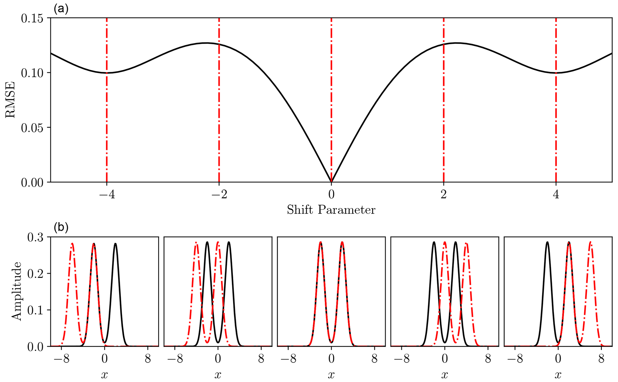
Figure 3 Root mean square error (a) between double Gaussians at a variety of time shifts (b, solid black and dash-dot red). Panel (b) corresponds to shift parameters indicated in panel a) with dash-dot red lines. In this example the situations shown in the far-left and far-right lower panels, with shift values of −4 and 4 respectively, both represent local minima in the RMSE function above, because the black curve has just a single peak aligned with the red dash-dot curve in each case, whereas the global minimum at shift value 0 has both peaks aligned.

An inadequate measure of fit can also lead to spurious local minima in the parameter estimation objective function, making local optimisation algorithms ineffectual (Engquist and Froese, 2014). These are especially common when the recorded signal is multi-modal. In these cases, displacement of such multi-modal features can lead to the “peaks” becoming incorrectly aligned and producing a locally low misfit (see Fig. 3).

Whether the misfit is unsuitable due to incorrect quantification of timing errors (Fig. 1), the double-penalty effect (Fig. 2), or local minima (Fig. 3), the key downfall of a point-wise metric can be traced to the same source: function comparisons occur in complete isolation, independently of all the other points. However, “cross-domain” comparisons are fundamentally necessary to recognise the temporal or spatial displacements which generate the problems. These types of issues are not exclusive to hydrology. For example, seismic signals can be compared by differences in amplitude or by considering differences in the travel times of seismic phases and thus timing errors. Local minima in the misfit function frequently arise when using amplitude-based misfit functions, this being the root of the infamous “cycle-skipping” problem commonly encountered in full waveform inversion, resulting from similar misalignment issues to those displayed in Fig. 3. Due to these similarities, we are motivated to explore the Wasserstein distance, derived from the field of optimal transport that has found recent use in seismology for quantifying waveform similarity in cases where amplitude-based misfit functions are inadequate (Engquist and Froese, 2014; Métivier et al., 2016).

While briefly addressed in Ehret and Zehe (2011), to the best of our knowledge the Wasserstein distance has had limited exposure in hydrology. It has been found to be beneficial for parameter estimation problems in geophysics, due to it comparing data holistically, rather than in isolated pairings, with this key property being what we seek to exploit (Engquist and Froese, 2014; Métivier et al., 2016). It has also been considered in the comparison of atmospheric contaminant fields (Farchi et al., 2016) and in some diagnostic data assimilation tasks with a similar rationale (Feyeux et al., 2018; Li et al., 2019).

Much like techniques considered in Roberts and Lean (2008) and Wernli et al. (2008), the Wasserstein distance is displacement-based, allowing more appropriate misfit quantification under temporal or spatial shifts. Its definition is derived from the concept of “transporting” one mass distribution onto the other and so naturally accounts for any such shifts. Consequentially, small timing errors for hydrograph comparison do not incur large penalties resulting from the misalignment of peaks in flow and are a more suitable measure of fit in the presence of timing errors than the RMSE or Nash–Sutcliffe efficiency. Use of the Wasserstein distance bears some similarity to the dynamic time-warping technique of Ouyang et al. (2010), the series distance (Ehret and Zehe, 2011), the hydrograph-matching algorithm of Ewen (2011), and the cumulative distribution method of Lerat and Anderssen (2015). While distinct from objective functions due to the need to understand the noise statistics of the data, some likelihood functions for Bayesian inference have attempted to account for temporally correlated residuals (e.g. Schoups and Vrugt, 2010; Vrugt et al., 2022). However, these generally operate directly in the point-wise residuals, while we use a different definition of “residual” based upon timing differences.

In this work, rather than detailing highly specific applications with complex models, we instead introduce methods that are suited for a range of tasks in (but not limited to) hydrology. The main goal is to highlight some of the key concepts of optimal transport and how they may find use in hydrology via simple, illustrative examples. The limitations of its use are also discussed and where further research is required. We also limit our experiments to one-dimensional problems, in particular the comparison of hydrographs. However, Sect. 1.2 details optimal transport in a more general sense, as it conserves its useful properties in multiple dimensions and so can also be used for comparing spatial fields.

1.2 Optimal transport

Optimal transport (OT) provides the numerical machinery for interrelating density functions. As distributions of water can be well represented as a density function with appropriate scaling, we suggest that OT gives the required tools for making more satisfactory comparisons than can be achieved by point-wise misfit functions.

Before the more modern interpretation with regards to density functions, OT originated with the work of Monge (1781), who was tasked with finding the most cost-effective way of filling a hole with a pile of dirt. OT is hence fundamentally concerned with reshaping one distribution of mass into another whilst minimising the requisite effort.

Little progress was made on generalised solution methods for this problem until it was rephrased by Kantorovich (1942). This forms the foundation of many modern computational methods (Peyré and Cuturi, 2019). However, we will introduce OT in a form closer to the original Monge definition, as this is based on continuous functions. While measured discretely, distributions of water have an underlying continuity in time or space, so this description is appropriate.

The central aspect of the Monge (1781) study was an optimal transport map acting as a directory between each location in the pile of dirt (known as the source) and an associated location in the hole (known as the target). By following this optimal map, the source distribution can be rearranged into the target distribution with minimal work. The relation between the source, target, and transport map is presented in Fig. 4.

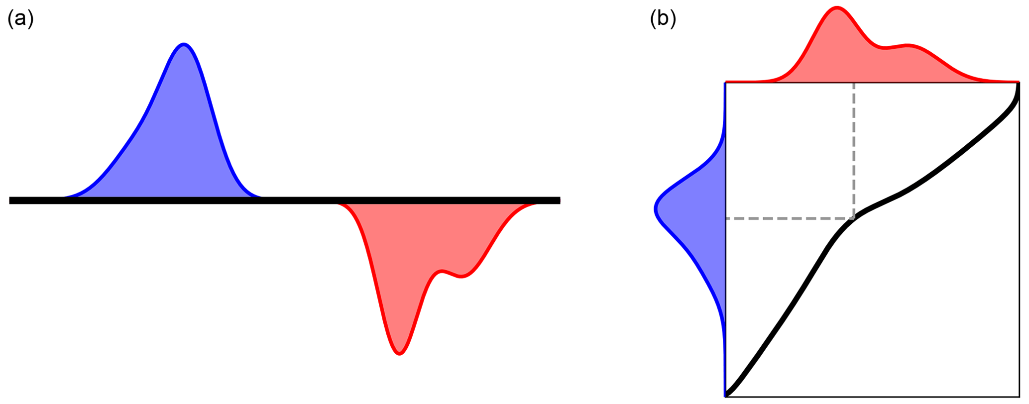
Figure 4 Panel (a) shows Monge's initial formulation of OT, with a source mass distribution (blue) and a target to be filled (red). Panel (b) shows the solution to the OT problem, with a transport map (black) transporting the source to the target. Dashed line shows the transport for a particular point.

Key restrictions for transport are mass conservation, meaning the source and target must have equal mass, and non-negativity, meaning that there cannot be negative mass at any point in either. These properties have led OT to be framed as between probability densities, as these naturally obey both requirements. If we denote the source as f and the target as g, these functions must satisfy Eqs. (2) and (3).

$$\begin{array}{}\text{(2)}& {\displaystyle }& {\displaystyle }\underset{\mathcal{X}}{\int }f\left(\mathit{x}\right)\mathrm{d}\mathit{x}\underset{\mathcal{Y}}{\int }g\left(\mathit{y}\right)\mathrm{d}\mathit{y}=\mathrm{1}\text{(3)}& {\displaystyle }& {\displaystyle }f\left(\mathit{x}\right)\ge \mathrm{0}\mathrm{for}\mathrm{all}\mathit{x}\in \mathcal{X},g\left(\mathit{y}\right)\ge \mathrm{0}\mathrm{for}\mathrm{all}\mathit{y}\in \mathcal{Y}\end{array}$$

Here, 𝒳 is the space over which f is defined, and 𝒴 is the space over which g is defined. In the case of hydrographs, these will be the time window over which the streamflow was measured, while for spatial fields, they will be the spatial extent of the recordings.

With the overarching goal of transporting f to g with minimal work, we must first define some notion of “effort” through the cost function, c(x,y), giving the amount of work it takes to transport one unit of mass from x to y. With this cost function in hand, the total cost of following some transport map T will be given by Eq. (4).

$$\begin{array}{}\text{(4)}& C\left(T\right)=\stackrel{\mathrm{cost}\mathrm{across}\mathit{all}\mathrm{points}}{\overbrace{\underset{\mathcal{X}}{\int }\underset{\mathrm{cost}\mathrm{for}\mathrm{a}\mathrm{single}\mathrm{point}}{\underbrace{c(\mathit{x},T(\mathit{x}\left)\right)f\left(\mathit{x}\right)\mathrm{d}\mathit{x}}}}}\end{array}$$

Finding the optimal transport map (denoted as T^*) therefore amounts to minimising Eq. (4), subject to the additional requirement that this map transports f exactly to g. Needless to say, this is a complicated functional minimisation problem and so will not be discussed in depth here as a simple analytical result is instead used. Direction to alternative methods is also provided in Sect. 2.1. As a mapping between densities, the optimal transport map is similar to transform-sampling methods such as inverse transform sampling or the trajectories in flow anamorphosis (van den Boogaart et al., 2017). However, we should reiterate that the optimal map differs in that it not only transforms between the densities, but also does so with minimal work.

Figure 5 Comparison of RMSE and squared 2-Wasserstein distance for the double-Gaussian problem displayed in Fig. 3. All misfits are scaled to a maximum of 1 for visualisation purposes.

Once found, the optimal transport map can be used to define the p-Wasserstein distance, the central concept of interest for this work. The p-Wasserstein distance (or simply the Wasserstein distance) is defined using the p norm raised to the pth power as the cost function, giving the cost of Eq. (5), where D is the dimensionality of the densities and sub-scripts are vector components.

$$\begin{array}{}\text{(5)}& c(\mathit{x},\mathit{y})=\sum _{d=\mathrm{1}}^D|{\mathit{x}}_d-{\mathit{y}}_d{|}^p=\Vert \mathit{x}-\mathit{y}{\Vert }_p^p\end{array}$$

The choice of p reflects how severely mass transport is to be penalised. That is, if p is large, mass transport across long distances will require more “work” relative to small transport distances and thus be avoided if possible. Upon finding the optimal transport map under the cost function Eq. (5), the Wasserstein distance is given by Eq. (6).

$$\begin{array}{}\text{(6)}& {\mathcal{W}}_p(f,g)={\left(\underset{\mathcal{X}}{\int }\Vert \mathit{x}-T^{*}\left(\mathit{x}\right){\Vert }_p^{p}f\left(\mathit{x}\right)\mathrm{d}\mathit{x}\right)}^{\frac{\mathrm{1}}{p}}\end{array}$$

The Wasserstein distance is symmetric and a true metric of the space of probability density functions, a deeper discussion of which can be found in Ambrosio et al. (2008) and Villani (2009). However, for the purposes of the present discussion, it is sufficient to state that similar mass distributions require little work to transport between them and thus have a low Wasserstein distance in comparison to dissimilar distributions, which require more work for transport. We will pay particular attention to the square of the 2-Wasserstein distance, ${\mathcal{W}}_{\mathrm{2}}^{\mathrm{2}}$, due to its convex properties that make it well suited for parameter estimation purposes (Engquist and Froese, 2014). We therefore set p=2 in Eqs. (5) and (6).

Armed with the Wasserstein distance, we can, for example, gauge the similarity of two hydrographs or a pair of precipitation fields. Again, note the key property that this is a global comparison, considering the total cost of transporting the entire source to the target rather than locally quantifying the distance using point-wise comparisons. It therefore naturally accounts for displacements through the transport map and assigns a more appropriate penalty for this type of error. We can see this through the simple numerical experiment in Fig. 5, where the Wasserstein distance provides a consistent interpretation of displacement, even when the features are not overlapping. It also mitigates the occurrence of local minima, due to cross-domain comparison. In a parameter estimation context, this provides a smooth, convex function well suited for gradient-based local optimisation methods.

These properties with respect to displacements have encouraged application in atmospheric chemistry and seismology alike (Farchi et al., 2016; Engquist and Froese, 2014; Métivier et al., 2016). However, while the Wasserstein distance naturally measures differences in shape and displacement, it is blind to differences in total mass between the source and target as they are scaled to unit mass prior to computation. Potential methods to counter this are proposed in Sect. 3 for applications where this may prove to be problematic.

1.3 Wasserstein barycentres

Beyond a straightforward measure of fit, the Wasserstein distance can also be used to define an “average” of density functions, known as the Wasserstein barycentre. The barycentre is the distribution that is the closest, in a Wasserstein sense, to the distributions we are finding the average of. This makes it the density that minimises a weighted sum of Wasserstein distances. If the ensemble of densities is denoted g_i and the barycentre is f, then f must obey both the requirements of density Eqs. (2) and (3) whilst minimising Eq. (7), with the relative weights of the component densities given by λ_i.

$$\begin{array}{}\text{(7)}& \min \left(\sum _{i=\mathrm{1}}^n{\mathit{\lambda }}_i{\mathcal{W}}_{\mathrm{2}}^{\mathrm{2}}\left(f,g_i\right)\right),\sum _{i=\mathrm{1}}^n{\mathit{\lambda }}_i=\mathrm{1}\end{array}$$

As OT makes cross-domain comparisons, the Wasserstein barycentre gives a more intuitive intermediate distribution when densities are separated in time or space. We can explore this through a simple example in Fig. 6.

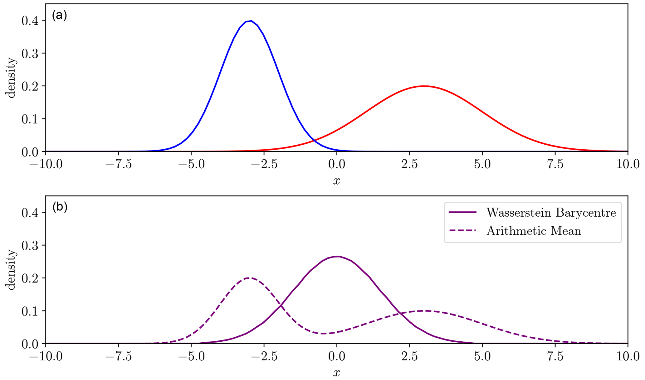
Figure 6 Two Gaussian density functions (blue, red, a) with one spatial/temporal dimension x. The Wasserstein barycentre of these densities (solid purple, b) and the mean (dashed purple, b).

Taking the arithmetic mean at each point of the two distributions gives a poor intermediate representation. Both of the densities have a single peak, but the intermediate one in Fig. 6 has two and so has not captured the characteristics of either. However, the Wasserstein distance provides a more satisfactory average conserving the shape of the peak. This again can be traced to how we define similarity. The conventional mean is defined with respect to amplitude, while the Wasserstein barycentre is an average with respect to the displacement pathway, also known as the geodesic (Ambrosio et al., 2008). Section 3 uses the Wasserstein barycentre to find the average hydrograph among an ensemble, each perhaps derived from a different climate or hydrological model, allowing conservation of peak shape and number in the case where equivalent peaks are equal in volume.

2 Computational methods

2.1 A brief survey

Now that the favourable properties of the Wasserstein distance for mass transport problems have been explored, we must discuss the computational methods. This aspect is perhaps the greatest difficulty in large-scale implementation. There are a variety of available techniques, some of which have been explored previously in similar applications, whilst others are a source of future discussion. A brief survey follows, with further details given in the associated references, many of which have unexplored potential for hydrological applications.

It was shown by Brenier (1991) that minimising Eq. (4) can be transformed into a partial differential equation when the squared Euclidean distance is used as the cost function. This can then be solved numerically; an example of one such solution is given in Benamou et al. (2014). This was the preferred method of Engquist and Froese (2014) and Yang et al. (2018) for comparison of seismic waveforms, although it is a technique not frequently seen in applied studies. The applicability of the method in seismology implies that this solution may be appropriate and warrant further consideration in the future for hydrology.

The more commonly used approach, especially for machine learning and graphics applications, is to use the Kantorovich formulation and thus consider the source and target densities to be discrete probability distributions, for which a linear program can be solved to obtain a transport plan (a generalised version of the transport map). While this is effective for a broader range of problems than the Monge–Ampère partial differential equation (PDE) that is specific to the squared Euclidean distance cost function, solving the linear program is computationally expensive and scales poorly with the size of the problem. This burden can be somewhat alleviated using the entropically regularised approach pioneered by Cuturi (2013), which has become the foundation for modern machine learning applications. Further efficiency can be achieved on regularly spaced data using the convolutional entropic regularisation developed in Solomon et al. (2015). Also derived from the entropically regularised approach are the stochastic optimisation methods of Genevay et al. (2016) and Seguy et al. (2018). These are particularly useful when samples can be drawn from the source and target densities.

There appears to be a bias in the literature towards discrete approaches, seemingly due to many machine learning problems not having a continuous interpretation, leaving the Monge–Ampère and related continuous approaches meaningless. We therefore should not be discouraged from using continuous methods for problems in the Earth sciences with spatial or temporal data, despite the relative lack of previous applications in the present literature. Indeed, we can see previous success of these methods in Engquist et al. (2016) and Yang et al. (2018).

2.2 One-dimensional transport

The method used in this work is structured around the special case of transport in one dimension, which accommodates a highly computationally efficient solution. When the source density f and target density g are both one-dimensional, the optimal transport map between them is given by Eq. (8).

$$\begin{array}{}\text{(8)}& T^{*}\left(x\right)=G^{-\mathrm{1}}\left(F\right(x\left)\right)\end{array}$$

Here, we have used F and G to represent the cumulative distribution functions (CDFs) of the source and target, these defined according to Eq. (9).

$$\begin{array}{}\text{(9)}& F\left(x\right)=\underset{-\mathrm{\infty }}{\overset{x}{\int }}f\left(x^{\prime }\right)\mathrm{d}{x}^{\prime },G\left(y\right)=\underset{-\mathrm{\infty }}{\overset{y}{\int }}g\left(y^{\prime }\right)\mathrm{d}{y}^{\prime }\end{array}$$

We should note here that in the one-dimensional case, using the optimal transport map is the same as the inverse transform-sampling method. Upon substituting the optimal map Eq. (8) into Eq. (6) to obtain the p-Wasserstein distance, a change in variables gives the simple form Eq. (10).

$$\begin{array}{}\text{(10)}& {\mathcal{W}}_p(f,g)={\left(\underset{\mathrm{0}}{\overset{\mathrm{1}}{\int }}{\left[F^{-\mathrm{1}}\left(s\right)-G^{-\mathrm{1}}\left(s\right)\right]}^p\mathrm{d}s\right)}^{\frac{\mathrm{1}}{p}}\end{array}$$

This reveals that, in the one-dimensional case, the Wasserstein distance is a measure of discrepancy between the inverse CDFs of the source and target. A visualisation of the one-dimensional Wasserstein distance under this interpretation is given in Fig. 7.

Figure 7 Process of moving from densities to 2-Wasserstein distance in one spatial/temporal dimension x. (a) Density functions from Fig. 4. (b) The cumulative distributions. (c) The inverse cumulative distributions with dashed lines showing transport pairs. (d) The difference between the inverse cumulative densities. (e) The area under the squared difference, giving the squared 2-Wasserstein distance.

In this study, we use the Nelder–Mead algorithm for optimisation, so the gradient of the Wasserstein distance is not required. However, if a gradient-based method were to be used, the derivative for the one-dimensional case can be derived directly from Eq. (10). Indeed, it was shown by Sambridge et al. (2022) that both the Wasserstein distance and its derivative can be computed through a sorting algorithm followed by a dot product. Engquist and Froese (2014) and Métivier et al. (2016) have also made use of the derivatives of the Wasserstein distance for parameter estimation, but they did not make use of the one-dimensional form.

Much like the Wasserstein distance, finding the Wasserstein barycentre of a series of densities is vastly simplified in one dimension. Rather than performing some type of optimisation scheme to minimise Eq. (7), we can find the barycentre directly from the inverse CDFs. Keeping the notation from Eq. (7), we have Eq. (11) (Bonneel et al., 2015).

$$\begin{array}{}\text{(11)}& F^{-\mathrm{1}}\left(s\right)=\sum _{i=\mathrm{1}}^n{\mathit{\lambda }}_i{G}_i^{-\mathrm{1}}\left(s\right),s\in [\mathrm{0},\mathrm{1}]\end{array}$$

That is, the inverse CDF of the barycentre is the weighted sum of the inverse CDFs of the component densities. Finding the barycentre then becomes a problem of converting an inverse CDF evaluated at a set of discrete points into a density function. Interchanging the (s, F⁻¹) coordinate pairs converts from the inverse CDF F⁻¹ to the CDF F. A finite-difference differentiation method can then be used to move from the CDF to the density function f. Finally, this can be interpolated into a smooth density function.

Overall, the Wasserstein barycentre definition of the average is equivalent to the histogram interpolation of Read (1999), although the author appears to have proposed this idea independently. The relation between the densities and their barycentre is displayed in Fig. 8.

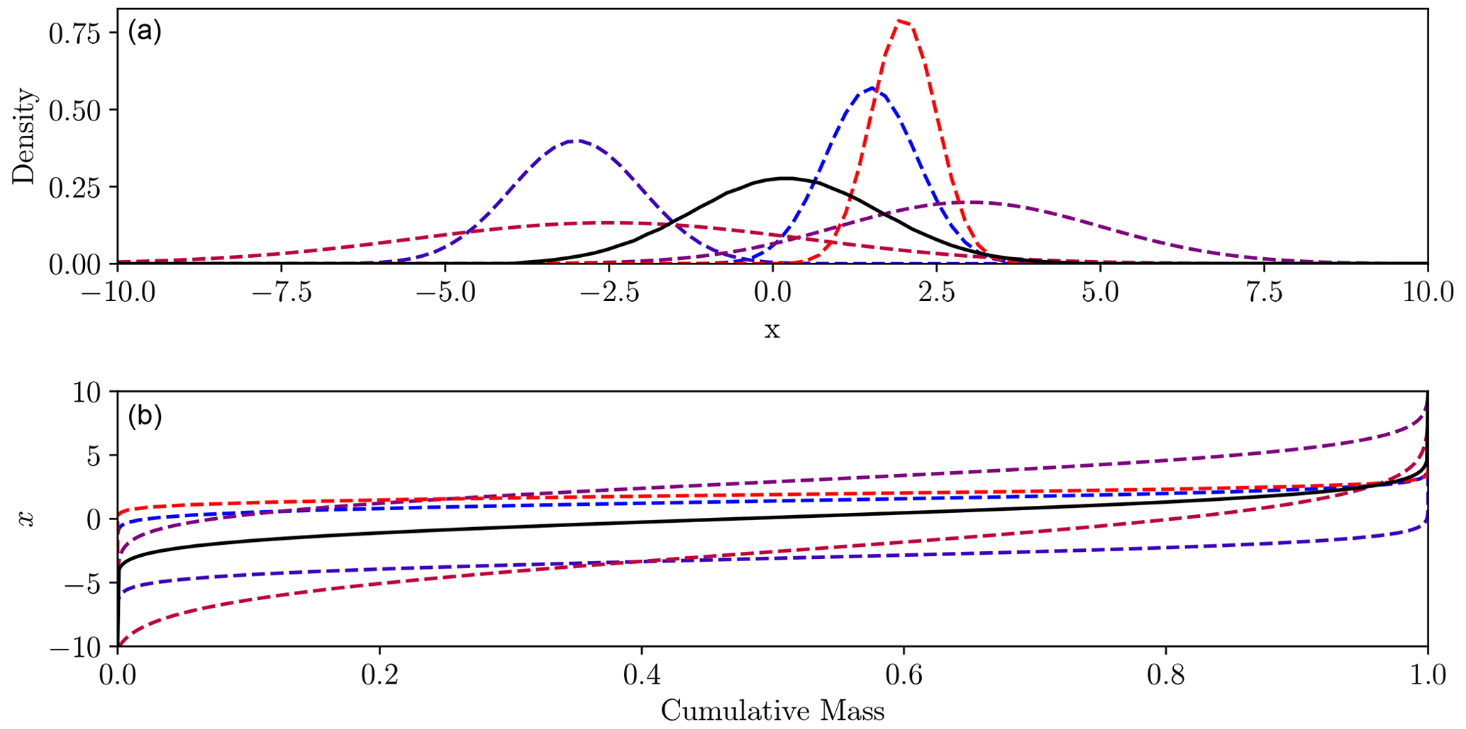
Figure 8 Method of finding the barycentre (solid black) from five Gaussian densities (dashed). Panel (a) shows density functions, panel (b) the inverse cumulative distributions. The mean of the inverse cumulative distributions is the cumulative distribution of the barycentre.

Again, it should be made clear that the computational results discussed here apply only to the one-dimensional case. Different methods must be used for multi-variate problems, a selection of which is given in Sect. 2.1. There is also the potential to use the alternative sliced Wasserstein distance (Rabin et al., 2011) or the more general continuous extension known as the radon Wasserstein distance (Bonneel et al., 2015), which both extend the one-dimensional results using one-dimensional projections of the multi-variate mass distribution. The radon and sliced Wasserstein distances display similar properties to the true Wasserstein distance and are a potential alternative to the more computationally expensive methods.

2.3 Adaptation to hydrology

OT is defined only for probability densities. For the applications we envisage, the non-negativity requirement will naturally be obeyed, as we are measuring inherently positive masses of water. The restriction of unit mass requires a little further consideration. We could take one of two differing philosophies: modify the data so they are compatible with OT or redefine OT such that it works with the type of data used. Here, we will consider both. Firstly, we can scale the water distributions such that they have unit mass and then compute the Wasserstein distance. The total mass of the densities is given by Eq. (12).

$$\begin{array}{}\text{(12)}& M_{\mathrm{f}}=\underset{\mathcal{X}}{\int }f\left(x\right)\mathrm{d}x,M_{\mathrm{g}}=\underset{\mathcal{Y}}{\int }g\left(y\right)\mathrm{d}y\end{array}$$

The scaling to unit mass is then given by Eq. (13).

$$\begin{array}{}\text{(13)}& \widehat{f}\left(x\right)={\displaystyle \frac{f\left(x\right)}{M_{\mathrm{f}}}},\widehat{g}\left(y\right)={\displaystyle \frac{g\left(y\right)}{M_{\mathrm{g}}}}\end{array}$$

Though this indeed makes the data compatible with OT, it also means that the Wasserstein distance becomes completely insensitive to differences in total mass. A multi-objective approach can be used to allow both shape (Wasserstein) and total mass (additional penalty term) to be accounted for, giving a misfit of the form Eq. (14).

$$\begin{array}{}\text{(14)}& {\mathcal{W}}_{\mathrm{2},\mathit{\gamma }}^{\mathrm{2}}={\mathcal{W}}_{\mathrm{2}}^{\mathrm{2}}(\widehat{f},\widehat{g})+\mathit{\gamma }h(f,g)\end{array}$$

Here, γ provides the relative importance of the total mass error compared to the Wasserstein distance, while h is the specific form of the penalty term. The quadratic function Eq. (15) is a simple choice for this penalty.

$$\begin{array}{}\text{(15)}& h(f,g)={\left(M_{\mathrm{f}}-M_{\mathrm{g}}\right)}^{\mathrm{2}}\end{array}$$

By selecting an appropriate weighting factor, we can develop a balanced misfit measure that contains the favourable properties of the Wasserstein distance whilst also removing the insensitivity to total mass differences. Note however that this weighting is a choice and so may require some tuning procedure to attain the desired balance between the two aspects of the fit.

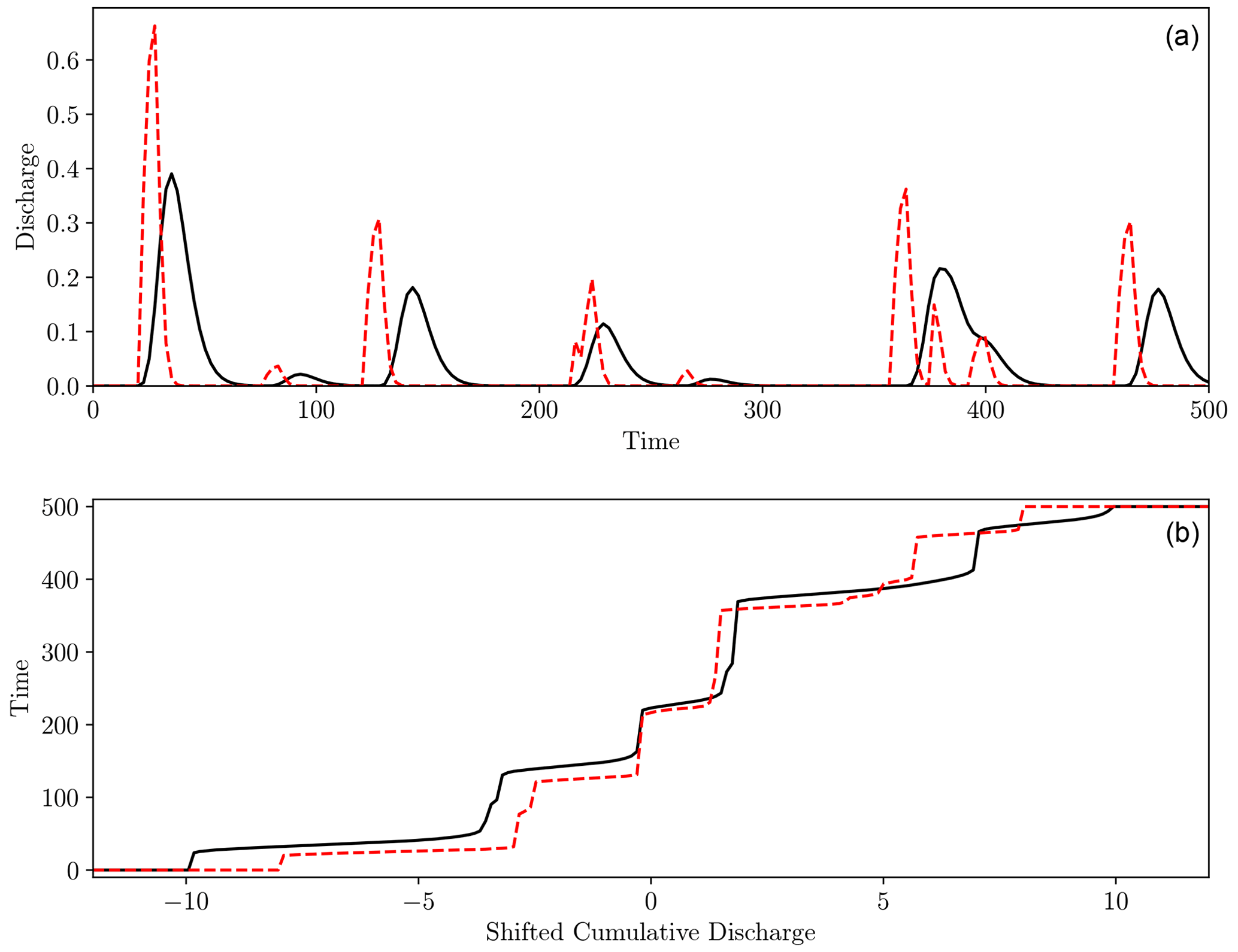
Figure 9 Visual representation of computing the hydrograph–Wasserstein distance. Panel (a) shows two synthetic hydrographs (dashed red and solid black) between which we want to compute the distance. Panel (b) shows the inverse shifted cumulative functions defined in Eqs. (18) and (19). Transport occurs between points vertically aligned in panel (b), forcing excess mass to be mapped to the boundaries.

We will now take the alternative approach of making a modification to OT to suit our hydrological purposes. The proposed result is derived for one-dimensional data but could potentially be extended to the multi-variate case in the same manner as the radon Wasserstein distance (Bonneel et al., 2015). We can build the new definition upon the foundation that we can compute the cumulative mass of a non-negative function, regardless of whether this mass sums to 1, and that this function will be monotonically increasing. The key step of a one-dimensional OT is that points of equal cumulative mass are matched in the optimal map (see Eq. 8 and Fig. 7). A similar concept with cumulative densities of arbitrary mass can be designed. Inspired by the ordinary Wasserstein distance, we can map the points of half-cumulative mass together (medians in the case of probability densities). To ensure these points are always aligned regardless of total mass, a shift can be applied such that the cumulative densities are centred at this halfway point using Eqs. (16) and (17).

$$\begin{array}{}\text{(16)}& {\displaystyle }& {\displaystyle }{F}_{\mathrm{s}}\left(x\right)=\left(\underset{-\mathrm{\infty }}{\overset{x}{\int }}f\left(x^{\prime }\right)\mathrm{d}{x}^{\prime }\right)-{\displaystyle \frac{M_{\mathrm{f}}}{\mathrm{2}}}\text{(17)}& {\displaystyle }& {\displaystyle }{G}_{\mathrm{s}}\left(y\right)=\left(\underset{-\mathrm{\infty }}{\overset{y}{\int }}g\left(y^{\prime }\right)\mathrm{d}{y}^{\prime }\right)-{\displaystyle \frac{M_{\mathrm{g}}}{\mathrm{2}}}\end{array}$$

For the matching of points of equal cumulative mass, the inverses of these are required. As we are working in the time window [0, T], we can limit the inverse to this range, giving the piece-wise functions Eqs. (18) and (19).

$$\begin{array}{}\text{(18)}& {\displaystyle }& {\displaystyle }{\stackrel{\mathrm{‾}}{F}}^{-\mathrm{1}}\left(s\right)=\left\{\begin{array}{ll}\mathrm{0},& s<-\frac{M_{\mathrm{f}}}{\mathrm{2}}\\ F_{\mathrm{s}}^{-\mathrm{1}}\left(s\right),& -\frac{M_{\mathrm{f}}}{\mathrm{2}}\le s\le \frac{M_{\mathrm{f}}}{\mathrm{2}}\\ T,& s>\frac{M_{\mathrm{f}}}{\mathrm{2}}\end{array}\right.\text{(19)}& {\displaystyle }& {\displaystyle }{\stackrel{\mathrm{‾}}{G}}^{-\mathrm{1}}\left(s\right)=\left\{\begin{array}{ll}\mathrm{0},& s<-\frac{M_{\mathrm{g}}}{\mathrm{2}}\\ G_{\mathrm{s}}^{-\mathrm{1}}\left(s\right),& -\frac{M_{\mathrm{g}}}{\mathrm{2}}\le s\le \frac{M_{\mathrm{g}}}{\mathrm{2}}\\ T,& s>\frac{M_{\mathrm{g}}}{\mathrm{2}}\end{array}\right.\end{array}$$

In a transport sense, we can see from Fig. 9 that this amounts to transporting the excess (or deficit) mass to (or from) the boundaries, which act as a source or sink to maintain the mass balance. In this case with a temporal domain, the boundaries are the start and end of the time window. The excess or deficit mass is therefore associated with times before t=0 or after t=500, whichever is closer in time. This makes it an alternative implementation of the method discussed in Farchi et al. (2016), who also proposed using sources or sinks at the boundaries of a spatial domain to complete the mass balance. Note that, like the traditional one-dimensional Wasserstein distance, this is a result that can be computed efficiently without the need to solve a partial differential equation, linear program, or iterative scheme.

Now that the mapping and form of the inverse cumulative distributions have been proposed, the modified Wasserstein distance under the interpretation that it is the total transport cost can be defined according to Eq. (20).

$$\begin{array}{}\text{(20)}& \mathcal{H}{\mathcal{W}}_{\mathrm{2}}^{\mathrm{2}}=\underset{-\mathrm{\infty }}{\overset{\mathrm{\infty }}{\int }}{\left[{\stackrel{\mathrm{‾}}{F}}^{-\mathrm{1}}\left(s\right)-{\stackrel{\mathrm{‾}}{G}}^{-\mathrm{1}}\left(s\right)\right]}^{\mathrm{2}}\mathrm{d}s\end{array}$$

We choose to label the misfit Eq. (20) the hydrograph–Wasserstein distance.

While Eq. (20) is expressed with infinite bounds, the integrand is only non-zero over the interval [$-M_{\max }/\mathrm{2}$, $M_{\max }/\mathrm{2}$], where $M_{\max }=\max \mathit{\{}{M}_{\mathrm{f}},M_{\mathrm{g}}\mathit{\}}$, and so can easily be computed numerically over this range.

The adjustment of barycentres for distributions of arbitrary total mass is much simpler. We can use the scaling defined in Eq. (13), find the barycentre of these distributions, and then scale the result such that its total mass is the average of the composite distributions. This is equivalent to replacing the Wasserstein distance in Eq. (7) with the penalised distance Eq. (14) under a quadratic penalty Eq. (15).

3 Rainfall–runoff modelling

3.1 Calibration

As a first application, the calibration of conceptual rainfall–runoff models using the Wasserstein distance as a minimisation objective was considered. This experiment is similar to that found in Lerat and Anderssen (2015) but uses all model parameters in the hydrological model.

A conceptual rainfall–runoff model gauges the relationship between a rainfall time series (hyetograph) and streamflow time series (hydrograph) for a particular watershed. By calibrating the model parameters to best capture this relationship, the model can be used for forecasting future streamflow under chosen rainfall conditions or to infer properties of the watershed itself. Automatic calibration methods seek to do this by minimising the discrepancy between the simulated streamflow from the rainfall–runoff model and the streamflow that was observed at gauging stations (Nash and Sutcliffe, 1970).

As hydrographs are a time series, the efficient one-dimensional techniques described in Sect. 2.2 were used. The application of the Wasserstein distance to this problem bears some similarity to the technique of dynamic time warping (DTW), an application of which to hydrology can be found in Ouyang et al. (2010), the series distance developed in Ehret and Zehe (2011), the cumulative distribution method in Lerat and Anderssen (2015), and the hydrograph-matching technique in Ewen (2011). These also strive to allow timing errors to be better accounted for when comparing hydrographs.

As was used by Lerat and Anderssen (2015), a non-linear storage model was employed to test the misfit functions. The storage in the model evolves according to the differential equation (Eq. 21).

$$\begin{array}{}\text{(21)}& {\displaystyle \frac{\mathrm{d}S}{\mathrm{d}t}}=m_{\mathrm{3}}r\left(t\right)-q\left(t\right)\end{array}$$

The outward streamflow flux is given by the non-linear model Eq. (22).

$$\begin{array}{}\text{(22)}& q\left(t\right)={\left({\displaystyle \frac{S\left(t\right)}{m\mathrm{1}}}\right)}^{m_{\mathrm{2}}}\end{array}$$

Using some initial volume of water in storage, we can update the storage and compute the streamflow at each time step for any given set of model parameters and hyetograph. This gives three model parameters (m₁, m₂, and m₃) that must be calibrated using given rainfall and runoff measurements. To work in a controlled environment while testing the main characteristics of the Wasserstein distance, synthetic rainfall events were used, and the model was used to generate the expected streamflow. We then attempted to recover the model parameters used to generate the synthetic observations.

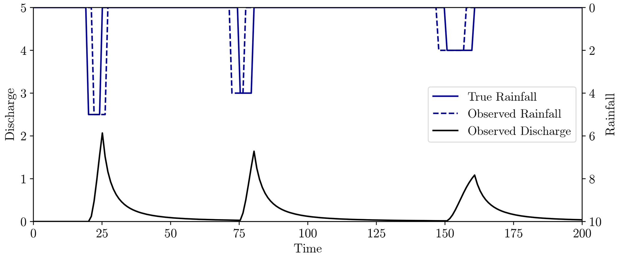
As precipitation is a more uncertain measurement than streamflow, we subjected the synthetic rainfall event to timing errors, recalling that these types of errors are poorly represented when using point-wise misfit metrics (Ehret and Zehe, 2011). Figure 10 shows the true synthetic hyetograph, the observed hyetograph corrupted by timing errors, and the streamflow generated by the true rainfall using the storage model defined in Eqs. (21) and (22).

Figure 10 True rainfall (solid blue) with timing errors in observations (dashed blue) and the observed hydrograph (black) produced from the true rainfall and storage model described by Eqs. (21) and (22) with model parameters (10, 2, 0.7).

We then calibrated the three model parameters to this streamflow using the erroneous rainfall measurements with a variety of misfit functions. Note that in the case of error-less data and a unique solution, all misfit functions discussed here would have a global minimum of 0 at the true model parameters. Optimisation was performed with the RMSE, Wasserstein distance (γ=10, 100), and hydrograph–Wasserstein distance using the Nelder–Mead algorithm, implemented through the scipy Python package (Nelder and Mead, 1965; Virtanen et al., 2020). Figures 11–13 show the misfit as a function of the model parameters, along with the true model parameters and the optimised parameters under each misfit.

Figure 11 Misfit surface as a function of m₁ and m₂ for each objective. Red circle marker represents true model parameters and red cross marker represents the minimised solution from the Nelder–Mead algorithm.

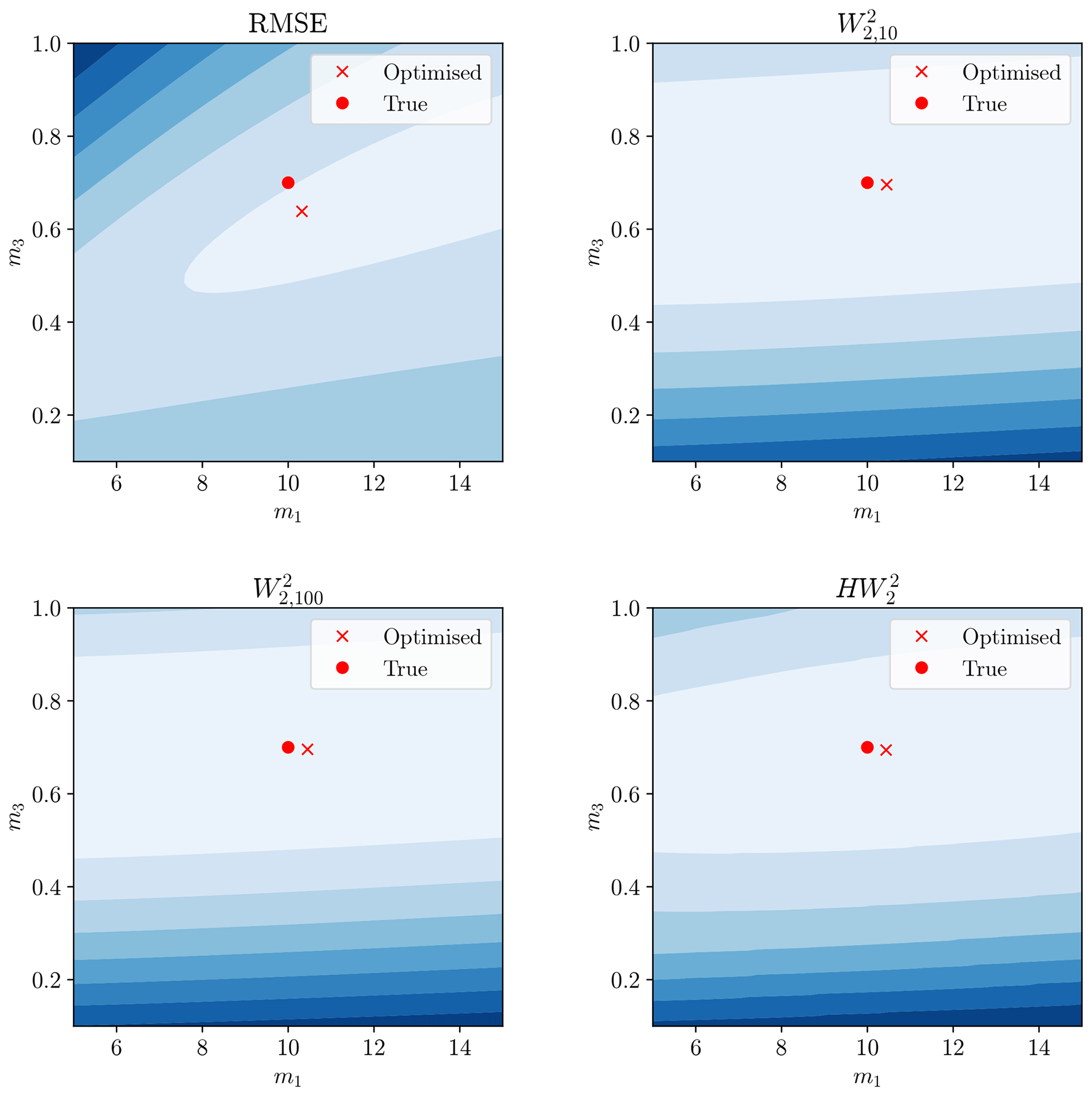
Figure 12 The same display as Fig. 11 but considering model parameters m₁ and m₃. Red circle still denotes true parameters and red cross the minimum of this surface.

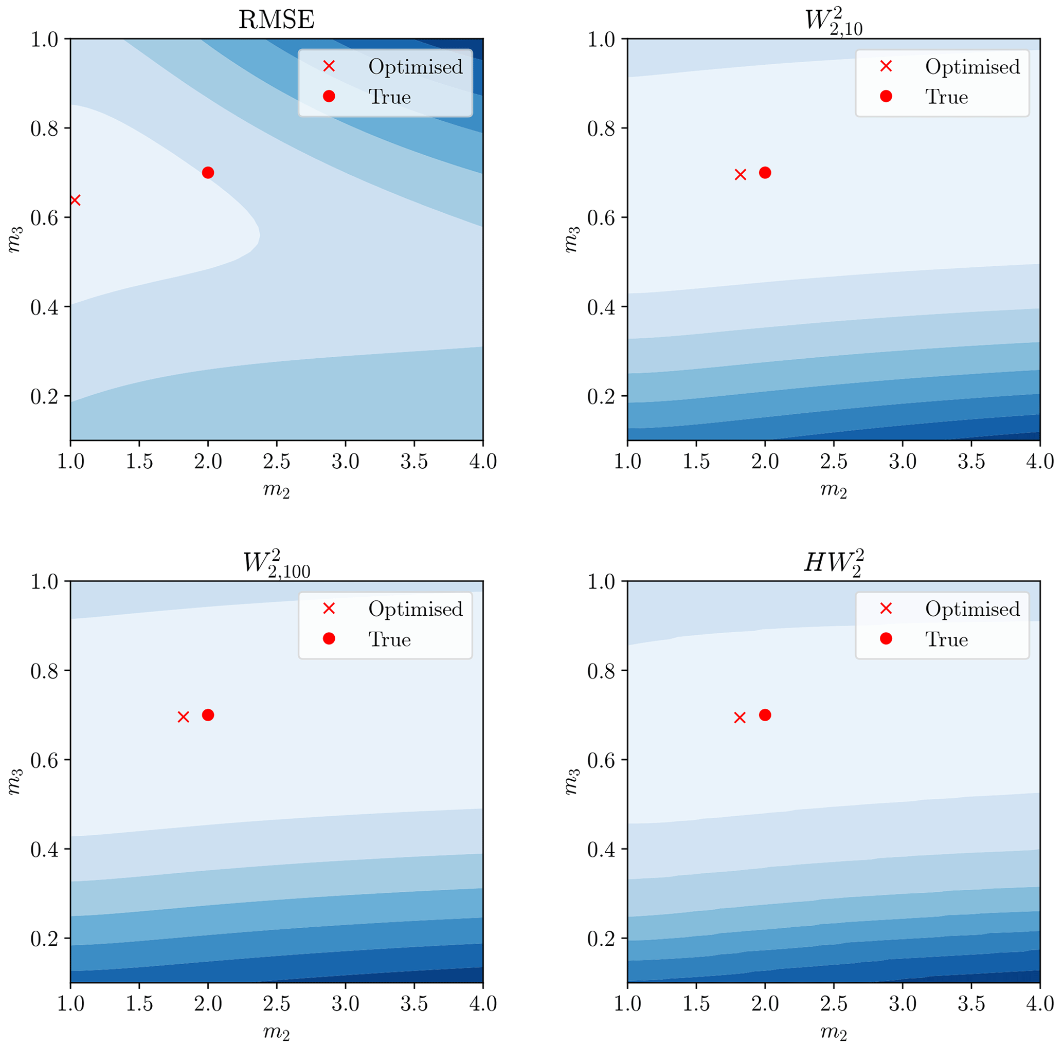
Figure 13 The same display as Fig. 11 but considering model parameters m₂ and m₃. Red circle still denotes true parameters and red cross the minimum of this surface.

The Wasserstein-based distances provided a misfit minimum closer to the true model parameters than the RMSE. A greater understanding of this can be garnered by examining the hydrographs produced by the calibrated model (Fig. 14).

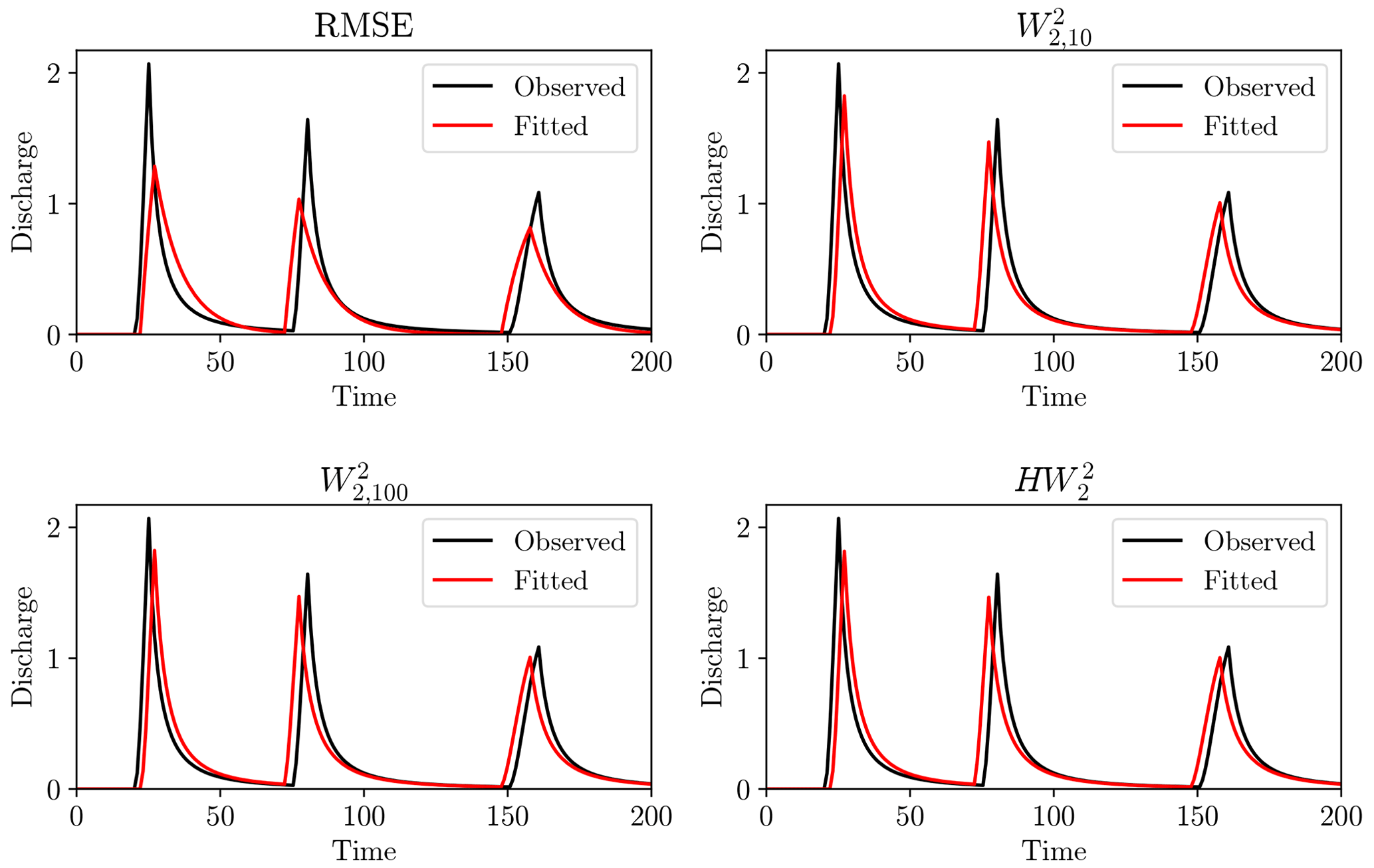
Figure 14 Output of the rainfall–runoff model for calibrated parameters under each objective function. Observations displayed in black and simulation in red.

The Wasserstein-based distances better recovered the model parameters and visually give a better hydrograph fit. The RMSE calibration underestimated the maximum flow peaks in favour of more sustained lowered flows. The reason for this can be traced back to Fig. 1, where misaligned steep peaks gave large residuals. This can be lessened by having wider peaks, even though this gives a visually less satisfactory hydrograph and poorer estimates of model parameters. We can conclude that, for this simple synthetic case study, the Wasserstein distance has promising attributes with respect to timing errors in hydrograph fitting.

Of course, this only shows the efficacy of the Wasserstein distance for one particular rainfall event. Random synthetic rainfall events were therefore generated using the method described in Appendix A, with the model calibrated to each event. The calibrated model parameters are compiled into boxplots in Fig. 15.

Figure 15 Calibrated model parameters for 500 rainfall events generated randomly using the method in Appendix A under the influence of timing errors. Optimisation used the Nelder–Mead algorithm initialised at the true model parameters of (10, 2, 0.7). Red solid line shows the median calibrated parameter, blue dash-dot line the true model parameter. Optimisation used RMSE, Wasserstein distance with γ=10, 100 penalty terms, and hydrograph–Wasserstein distance.

Whilst still having some variability and bias, the Wasserstein-based distances performed significantly better across the 500 trials, with a median result closer to the true value for all parameters and lowered variability. The ordinary Wasserstein distance outperformed the hydrograph–Wasserstein distance for this model. The size of the penalty-weighting factor γ had little effect on the location of the optimum for the Wasserstein distance but altered the shape of the misfit surface (see Figs. 11–13).

The better performance of the penalised Wasserstein distance compared to the hydrograph–Wasserstein distance may be due to the form of this model. As m₁ and m₂ purely control hydrograph shape and m₃ purely controls total output mass, there is a complete separation in which model parameters affect each aspect of the misfit; that is, no model parameter simultaneously influences both the Wasserstein distance and the mass balance penalty term unless the change in m₁ or m₂ moves mass outside of the measured time window.

Subsequently, there is no “trade-off” between lowering the Wasserstein distance or penalty term; both are always possible as the model parameters only influence both if mass is pushed outside the time window (hence there being any variability in the m₃ panel of Fig. 15).

If there were model parameters that influenced both shape and total mass, this separation of aspects would not be present, and the magnitude of γ may have increased importance due to the trade-off between fitting the shape and balancing the mass of the hydrographs when tuning a model parameter.

3.2 Instantaneous unit hydrograph model

Section 3.1 showed that the Wasserstein distance gives a better account for timing errors than can be made from point-wise metrics. The effect of delay times from within the hydrological model itself is now considered. A simple unit hydrograph model was used to generate such delays between rainfall and the associated streamflow. The instantaneous unit hydrograph (IUH) is defined as the streamflow response for a unit impulse of effective rainfall over the catchment. Under the assumption of a linear response, the stream hydrograph can be modelled via a convolution of the rainfall and IUH, giving the model Eq. (23).

$$\begin{array}{}\text{(23)}& q\left(t\right)=\underset{-\mathrm{\infty }}{\overset{\mathrm{\infty }}{\int }}u(t-s)r\left(s\right)\mathrm{d}s=u\left(t\right)\cdot r\left(t\right)\end{array}$$

In reality, we can only measure the streamflow and rainfall, leaving us to infer the IUH from such measurements. To enforce some set of desired characteristics on the IUH, such as smoothness, positivity, and unit mass, it can be restricted to belonging to a parametric set, each of which is of the correct form. A commonly used synthetic unit hydrograph is the Nash hydrograph (Nash, 1957). This assumes that the watershed is composed of a series of linear reservoirs, giving a unit hydrograph of the form Eq. (24), where Γ is the Gamma function.

$$\begin{array}{}\text{(24)}& u\left(t\right)={\displaystyle \frac{\mathrm{1}}{\mathrm{\Gamma }\left(k\right){\mathit{\theta }}^k}}{t}^{k-\mathrm{1}}{e}^{-t/\mathit{\theta }}\end{array}$$

This leaves us with two parameters, θ and k, to calibrate. Although there are multiple existing ways of solving this problem so the OT approach is not necessarily warranted, this application has some of the key features we would like to explore more generally in rainfall–runoff model calibration whilst keeping the model structure simple.

The effective rainfall time series was generated using the method described in Appendix A with 10 rainfall events, giving the output displayed in Fig. 16, where the true model parameters of the IUH are θ=3, k=5.

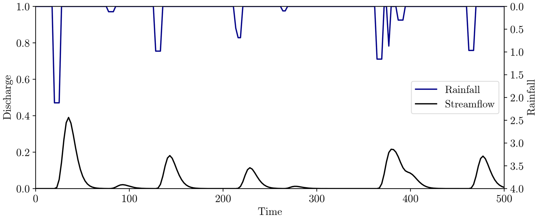
Figure 16 Effective rainfall (top, blue) and observed streamflow (bottom, black) for the test problem. Rainfall was generated using the method described in Appendix A with 10 rainfall events of maximum length five time units. The streamflow was generated using the unit hydrograph model Eq. (24) with model parameters (3, 5).

The behaviours of both the Wasserstein distance and the RMSE were explored here with respect to the time delays induced by the IUH model. The misfit as a function of the two model parameters is shown in the left-hand-side panels of Fig. 17.

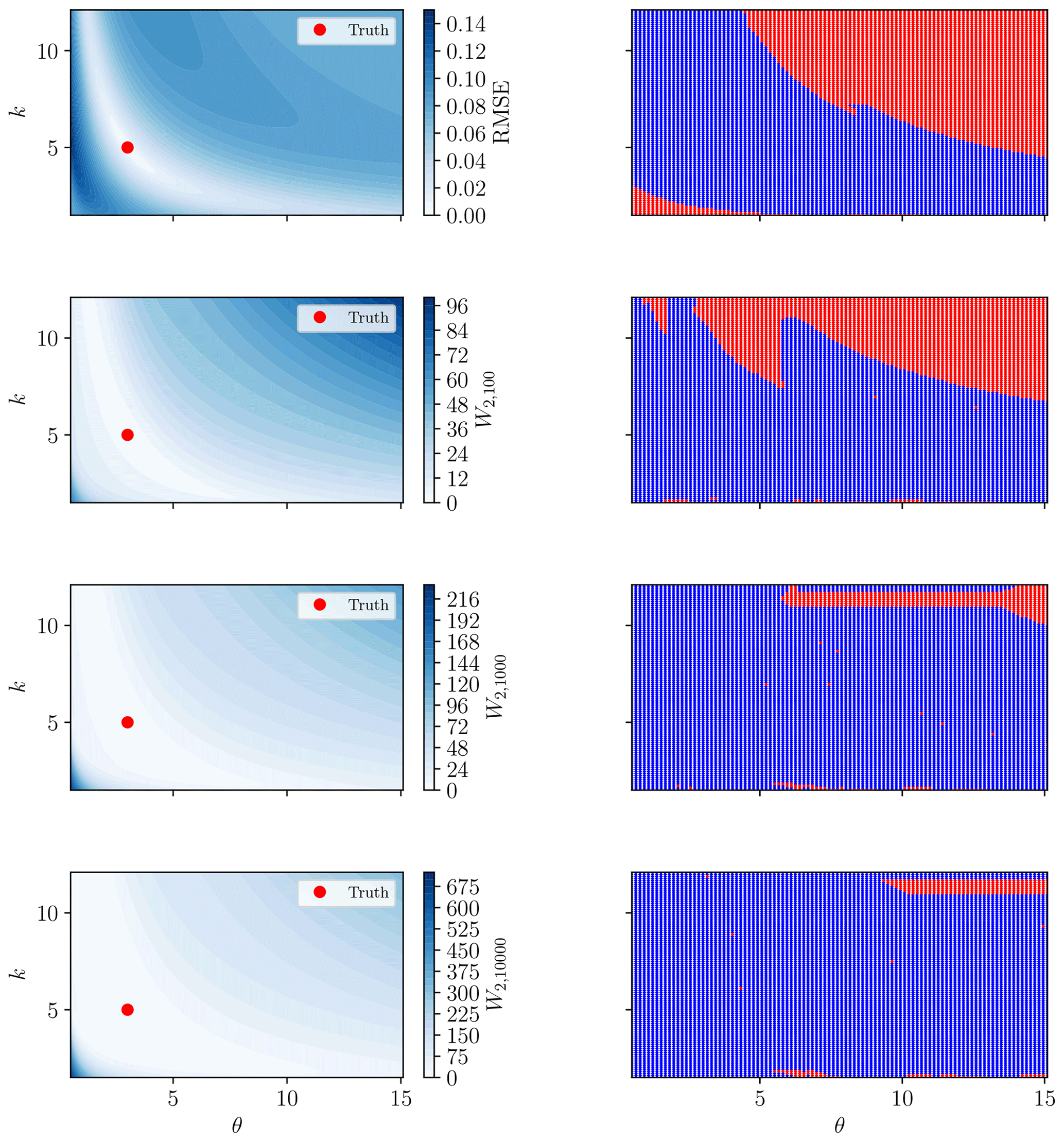
Figure 17 Root mean square error and 2-Wasserstein (with γ=100, 1000, 10 000) misfit surfaces for the rainfall event in Fig. 16 and the unit hydrograph model (Eq. 24) (left-hand-side panels). Red marker shows the true solution. The RMSE surface displays local minima in the lower-left and upper-right corners, where poor convergence is observed. The right-hand-side panels show whether convergence criteria were met (blue) or not (red) for each model initialisation.

The key difference between the misfit surfaces in Fig. 17 is that local optimisation methods will converge for a greater number of starting locations towards the true optimal point (marked red in the left-hand-side panels) when using the Wasserstein-based distance. While many initial estimates with the RMSE will also converge to this same point, there are also alternative minimal points to which the optimisation scheme may converge. A grid of starting estimates of the model parameters was used to examine this more concretely in the right-hand-side panels of Fig. 17. These panels show the convergence properties according to the initial model parameter estimate for the RMSE and the Wasserstein distance for three choices of γ. Convergence is defined as the optimised model m^* satisfying $\Vert m^{*}-m_{\mathrm{true}}{\Vert }_{\mathrm{2}}<\mathrm{0.001}$, where m_true is the true solution, denoted as the red points in the left-hand-side panels of Fig. 17.

From Fig. 17, there is a clearly defined “basin of attraction” about the optimal solution for RMSE, beyond which local optimisation algorithms will not converge. This matches well with the corresponding misfit surface in the top left-hand-side panel. The Wasserstein distance converged for a greater number of initial estimates, with improvement seen for a larger choice of γ. This is likely due to the low sensitivity of the misfit surface within the “valley” about the optimal solution (visualised as the white region in Fig. 17). The larger value of γ increases the sensitivity (gradient of the misfit surface) and potentially prevents early termination of the optimisation algorithm.

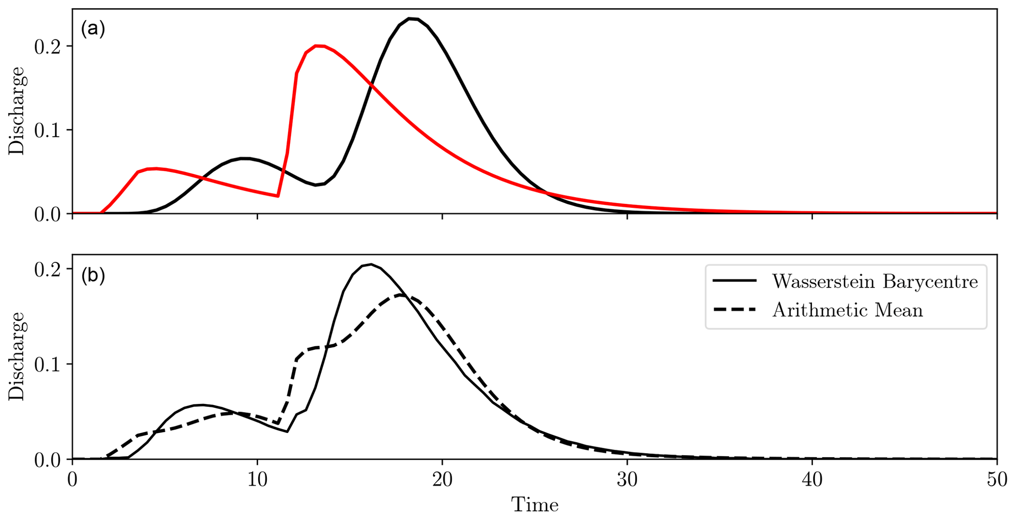
Figure 18 Two hydrographs for the same rainfall event but with different hydrological models (a, black and red solid lines). Panel (b) shows the Wasserstein barycentre in solid black and the mean in dashed black.

We do acknowledge that it takes a relatively poor initial estimate of the model parameters to become trapped in a local minimum for this IUH model. Indeed, with only two model parameters, a brute force global optimisation method is certainly feasible. Furthermore, a good initial estimate may be generated using the method of moments for the Nash IUH. However, these results show the ability of the Wasserstein distance to recognise the error in improperly aligned peak flows.

The power of the Wasserstein distance may come to the fore when a more complex watershed and thus model are used, perhaps producing multiple pulses per rainfall event and yielding multiple peaks in the IUH. These results also capture the general behaviour of models possessing significant delay times, allowing the simulated hydrograph to “shift” in time across the observations, in a similar manner to Fig. 3.

3.3 Hydrograph barycentres

Beyond the use of the Wasserstein distance purely as an objective function, attention will now be turned to the application of Wasserstein barycentres to hydrology, using hydrographs as the object of study. The power of the Wasserstein barycentre is that it gives a notion of an “average” when features have been displaced.

This means that an ensemble of hydrographs describing the same event, perhaps with different climate or hydrological models, can be “averaged” into a single hydrograph that carries characteristics of each ensemble member. Note that this will only be true if the main source of difference between ensemble members is timing and peak shape differences rather than peak volume differences.

To test this premise, two different IUH models were applied to the same synthetic rainfall event, giving the differing hydrographs shown in Fig. 18a. As they were from the same rainfall event and a unit hydrograph model was used, the volumes of the peaks in each hydrograph were approximately the same, with only the shape and timing differing, and so this is suitable for the Wasserstein approach. Figure 18b compares the Wasserstein barycentre with the mean of the hydrographs.

Unlike the ordinary mean, the Wasserstein distance captured the correct number and general characteristics of the peak flows. Again, this is built on the assumption that the peaks of each hydrograph mainly differ in shape and timing but not volume. If they differed in volume, the barycentre could exhibit peaks in unusual locations, as the mass is being “viewed” halfway through transport across the domain.

Consider the two hydrographs shown in Fig. 19a. They are the same in timing but differ in the volume of water. In this case, the regular mean gave a much better notion of the average, as the difference between the hydrographs is better explained in terms of amplitude rather than displacement, as was the case in Fig. 18.

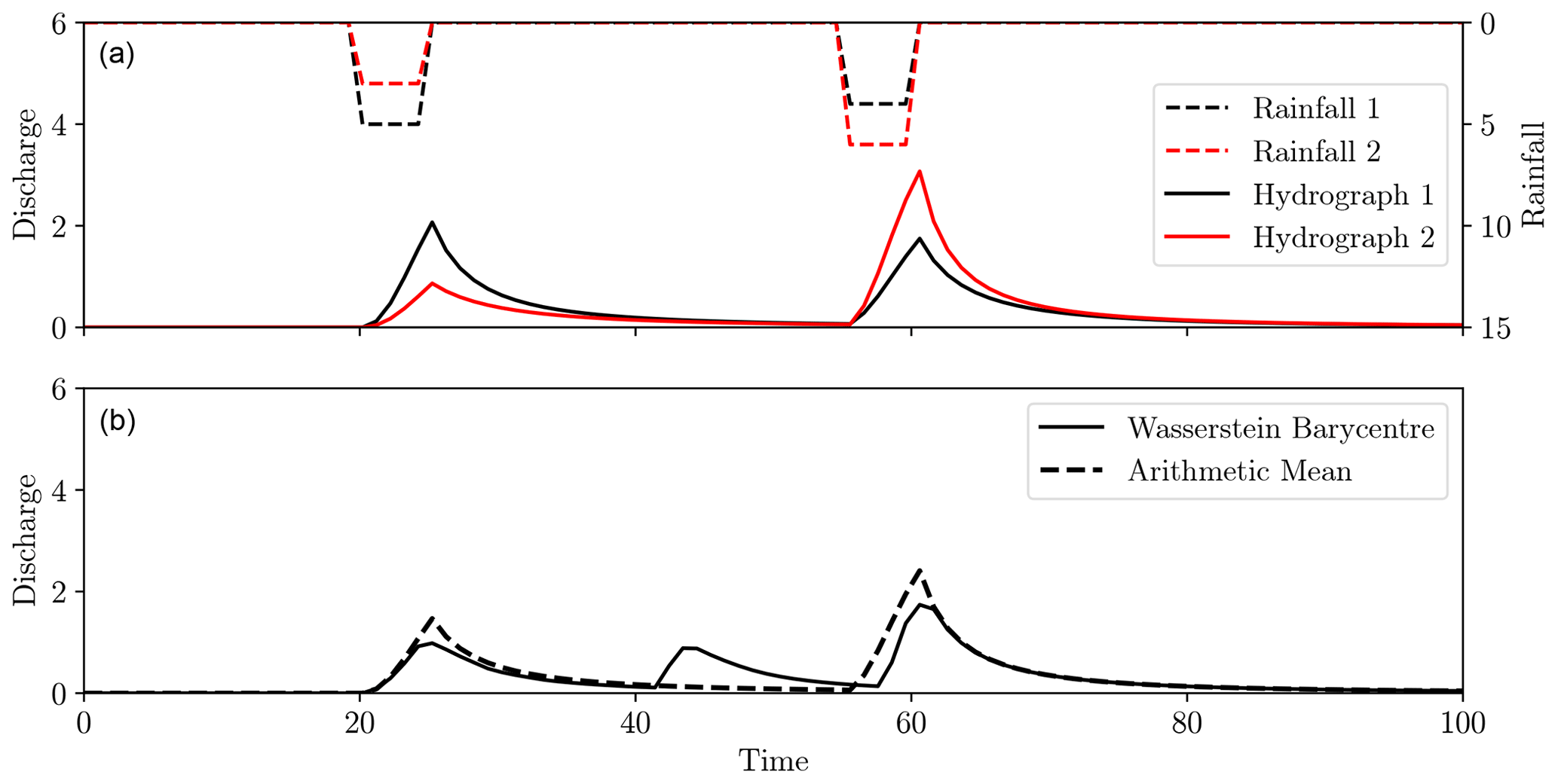
Figure 19 The same hydrological model applied to rainfall events differing in amplitude (dashed black and red, inverted plots in panel a), giving hydrograph differences purely in amplitude (solid black and red, a). Panel (b) shows the mean (dashed black) and Wasserstein barycentre (black).

We therefore see that while the Wasserstein barycentre is well suited for an ensemble of hydrographs with differing peak flow timings, it is not well suited for amplitude differences. This is to be expected from its definition. We therefore suggest that the conventional mean is best suited for an ensemble with differing amplitudes but consistent timings, whilst the Wasserstein barycentre is appropriate when timing is variable, but volumes in peak flows are consistent.

4 Conclusions

Quantifying the similarity of temporal or spatial distributions of water occupies an important role within hydrology. The way in which a “good” fit is defined directly influences the character of the results. Many commonly used misfit functions, such as root mean square error and Nash–Sutcliffe efficiency, quantify fit by considering differences in amplitude. While this is perfectly acceptable when errors are restricted to amplitude, these measures of misfit do not well quantify displacement errors.

In this work, we have suggested the Wasserstein distance, derived from optimal transport, as a candidate misfit function for applications where displacement or timing errors are prominent. This quantifies difference in terms of the effort required to transform one mass distribution into another. A modification of traditional OT and the associated “hydrograph–Wasserstein distance” was also developed.

While the Wasserstein-based measures certainly gave better calibration results than RMSE, there was still a slight bias towards peaks of reduced amplitudes, although to a much lesser extent. Some type of multi-objective method may circumvent this by using a measure comparing the amplitude of peak flows. Although the Wasserstein distance with a penalty term outperformed the hydrograph–Wasserstein distance for these synthetic tests, there may be broader implications for this second misfit function. Very little interest has been given thus far to the modification of OT for particular applications, with most preferring to force data into the density function mould. Other ways of modifying whilst still capturing the essence of OT are therefore a key point of further research, as they may allow the simultaneous capture of displacement and total mass errors without the need for a user-defined weighting term between the aspects. Focus in this work has been placed upon the Wasserstein distance rather than the optimal map from which it is derived. There is unexplored potential in this optimal map for providing a two-way mapping between collected data and a reference distribution in a similar vein to flow anamorphosis (van den Boogaart et al., 2017; Talebi et al., 2019).

As proposed by Ehret and Zehe (2011), a major drawback of the Wasserstein distance for hydrographs is the mapping of water masses between functionally different parts of the hydrographs. For example, if the modelled volume of a particular storm event exceeds the observations, this excess water is mapped to the next (and unrelated) storm event. If the storm events are separated by long dry periods, a large transport cost would be incurred by moving the mass between the events. Therefore, when fitting multiple events interspersed with dry spells, it may be more appropriate to segment the hydrographs into each discrete event and compute the Wasserstein distance individually within each time window to prevent this mapping between events. The objective function would then become the summation of the Wasserstein distances for each time segment. This would not be possible for wet periods with overlapping rainfall events, but the penalty for transporting mass between events would be much smaller in this case as they occur closer together in time.

It is also important to remember that, for more complex models and data, we cannot expect the Wasserstein distance to capture all aspects of fit. Much like the amplitude-based metrics, it prioritises particular aspects of fit and has the potential to yield large-amplitude errors at specific points as long as mass has not been shifted far from the target location. We are therefore led back to our introductory question of what is a good “fit”? If we know, or expect, timing or spatial displacement errors in our measurements or model output, a transport-based definition of fit would seem appropriate. However, this may not be the case when other types of errors are at play. A multi-objective approach may therefore still be a necessary and even encouraged technique. The results here do however show that the Wasserstein distance is suitable for quantifying displacement errors and so is a valuable addition to the toolbox of misfit functions in operation in hydrology.

Appendix A: Random rainfall generation

For the synthetic experiments, a method for generating random rainfall events was required. This is done by first setting a time window length. Let this window be the interval [0, T], where any units can be used.

A number of rainfall events N is then specified by the user. The start time of each of these rainfall events is chosen from a random uniform distribution within the time window. That is, if the start time of the ith event is denoted as s_i, then

$$\begin{array}{}\text{(A1)}& s_i\sim U(\mathrm{0},T).\end{array}$$

The length of each of these rainfall events is then chosen from a uniform distribution of specified maximum length t_max, so the length of the ith event is given by

$$\begin{array}{}\text{(A2)}& l_i\sim U\left(\mathrm{0},t_{\max }\right).\end{array}$$

Together, these give start and end times for each storm, where the end time e_i is given by

$$\begin{array}{}\text{(A3)}& e_i=s_i+l_i.\end{array}$$

The intensity of the rainfall r_i for each storm is chosen independently from an exponential distribution with rate parameter λ.

$$\begin{array}{}\text{(A4)}& r_i\sim \mathrm{Exponential}\left(\mathit{\lambda }\right)\end{array}$$

In this study, we set λ=1, as the rainfall units are arbitrary.

To corrupt the measurements with timing errors, the timing of each storm is shifted independently by a number δ_i drawn from a uniform distribution ranging between a positive and negative maximum time shift, δ_max, so that

$$\begin{array}{}\text{(A5)}& {\mathit{\delta }}_i\sim U\left(-{\mathit{\delta }}_{\max },{\mathit{\delta }}_{\max }\right).\end{array}$$

This gives the altered start and end times for each storm as

$$\begin{array}{}\text{(A6)}& {\displaystyle }& {\displaystyle }{s}_i^{\prime }=s_i+{\mathit{\delta }}_i,\text{(A7)}& {\displaystyle }& {\displaystyle }{e}_i^{\prime }=e_i+{\mathit{\delta }}_i.\end{array}$$

Between the start and end times of each rainfall event, constant rainfall of the randomly chosen intensity is applied. If rainfall events overlap, the intensities are added for this cross-over period.