A robust gap-filling approach for European Space Agency Climate Change Initiative (ESA CCI) soil moisture integrating satellite observations, model-driven knowledge, and spatiotemporal machine learning

Spatiotemporally continuous soil moisture (SM) data are increasingly in demand for ecological and hydrological research. Satellite remote sensing has potential for mapping SM, but the continuity of satellite-derived SM is hampered by data gaps resulting from inadequate satellite coverage, snow cover, frozen soil, radio-frequency interference, and so on. Therefore, we propose a new gap-filling approach to reconstruct daily SM time series using the European Space Agency Climate Change Initiative (ESA CCI). The developed approach integrates satellite observations, model-driven knowledge, and a machine learning algorithm that leverages both spatial and temporal domains. Taking SM in China as an example, the reconstructed SM showed high accuracy when validated against multiple sets of in situ measurements, with a root mean square error (RMSE) and a mean absolute error (MAE) of 0.09–0.14 and 0.07–0.13 cm³ cm⁻³, respectively. Further evaluation with a 10-fold cross-validation revealed median values of the coefficient of determination (R²), RMSE, and MAE of 0.56, 0.025, and 0.019 cm³ cm⁻³, respectively. The reconstructive performance was noticeably reduced both when excluding one explanatory variable and keeping the other variables unchanged and when removing the spatiotemporal domain strategy or the residual calibration procedure. In comparison with gap-filled SM data based on a satellite-derived diurnal temperature range (DTR), the gap-filled SM data from bias-corrected model-derived DTRs exhibited relatively lower accuracy but higher spatial coverage. Application of our gap-filling approach to long-term SM datasets (2005–2015) produced a promising result (R²=0.72). A more accurate trend was achieved relative to that of the original CCI SM when assessed with in situ measurements (i.e., 0.49 versus 0.28, respectively, in terms of R²). Our findings indicate the feasibility of integrating satellite observations, model-driven knowledge, and spatiotemporal machine learning to fill gaps in short- and long-term SM time series, thereby providing a potential avenue for applications to similar studies.

1 Introduction

As an essential component of land–atmosphere interactions, soil moisture (SM) substantially impacts the energy, water, and carbon cycles. It plays important roles in hydrological, environmental, and agricultural applications such as evapotranspiration (ET) estimation (Detto et al., 2006), drought assessment (Wang et al., 2011), and flood forecasting (Wanders et al., 2014). SM has been declared by the Global Climate Observing System (GCOS) and the United Nations Framework Convention on Climate Change (UNFCCC) as one of the 50 vital variables in terrestrial domains (Mason et al., 2010). Availability of spatially and temporally continuous daily all-weather SM data could facilitate improved understanding of ecological and hydrological processes; therefore, provision of a reliable SM dataset is urgently demanded.

Various methods are available for collecting SM data. In situ measurements can capture the temporal variability of SM at the station scale, and many networks designed for such in situ observations have been installed regionally, nationally, and globally, e.g., the crop growth and farmland SM database in China, the North American Soil Moisture Database in North America, and the International Soil Moisture Network (ISMN) (Schaake et al., 2004; Dorigo et al., 2011, 2021). Nevertheless, owing to the limited number of ground stations, obtaining spatially continuous SM measurements across large-scale regions remains a challenge. In addition to ground-based observations, SM can be simulated using numerical models. The Global Land Data Assimilation System (GLDAS) and the European Centre for Medium-Range Weather Forecasts (ECMWF) fifth-generation global atmospheric reanalysis (ERA-5) can model the soil moisture values that have sufficient spatial coverage (Chen et al., 2013; Reichle et al., 2011). However, such model simulations tend to be sensitive to uncertainties related to model structure, forcing, and parameterization (Prihodko et al., 2008; Dorigo et al., 2017).

Satellite observation is considered a powerful technique for retrieving surface SM data, especially given recent improvements in sensor technology. Some SM-dedicated satellites, e.g., the Advanced Microwave Scanning Radiometer-Earth Observation System (AMSR-E) and the Advanced Scatterometer (ASCAT), have used the higher C-band and X-band microwave frequencies to collect SM signals. Despite the sensitivity of satellite-derived SM data to atmospheric variability and vegetation coverage, satellites operating with lower L-band radiometers, such as Soil Moisture and Ocean Salinity (SMOS) (Kerr et al., 2001) and Soil Moisture Active and Passive (SMAP) (Entekhabi et al., 2010), have exhibited great potential for collecting SM data because of the strong capacity of wavelengths in the L-band frequency range to penetrate vegetation. A case worth noting is that the European Space Agency Climate Change Initiative (ESA CCI) has generated one set of a global SM dataset (Gruber et al., 2019; Dorigo et al., 2017). This CCI SM product blends a series of SM products from active–passive microwave satellite sensors, giving it one complete and consistent observational SM record. Previous studies have revealed reasonable correlation between the CCI SM dataset and in situ measurements obtained over different regions (Dorigo et al., 2015).

The gap issues that remain in current satellite-based SM products relate to various factors such as snow cover, frozen soil, radio-frequency interference, and orbital changes in the satellite sensors (Dorigo et al., 2017). Considerable effort has been dedicated to filling missing values in satellite-derived SM datasets. Traditional interpolation approaches that are applied to fill gaps rely on the spatial or temporal patterns of the target variable, such as inverse distance weighting and cokriging (Yao et al., 2013; Ford and Quiring, 2014). Other studies (Leng et al., 2017; Llamas et al., 2020; Meng et al., 2021) have focused on the use of statistical methods that mainly depend on the statistical and physical relationships between target variables and explanatory variables. Only recently have machine learning strategies been introduced to the problem of gap filling in relation to satellite-derived datasets (Zhang et al., 2021a, b; Bessenbacher et al., 2022b). Such methods have the capacity to depict complex relationships of target variables and explanatory variables. For instance, Elsaadani et al. (2021) assessed the spatiotemporal deep learning method for filling the gaps in soil moisture observations, and Li et al. (2021b, 2022c) further improved satellite soil moisture prediction using the deep learning model. In comparison with statistical-based models, machine learning models might be more flexible and robust, especially with regard to complex scenes and extended coverage (Reichstein et al., 2019).

Most SM gap-filling studies rely on explanatory variables that are required in describing SM dynamics. In addition to satellite-derived vegetation indexes (e.g., normalized difference vegetation index, NDVI, and enhanced vegetation index, EVI), surface albedo, and land surface temperature (LST), various climatic and geographical factors have been employed in such studies (Almendra-Martín et al., 2021; Cui et al., 2019; Jing et al., 2018). Nevertheless, although appropriate for use in certain regions, most of those variables are less suitable for use in heterogeneous regions and for extended coverage. For example, previous studies (Song et al., 2021; Liu et al., 2020b) that focused on the NDVI and LST tended to achieve better performance in depicting SM in arid and semi-arid regions but produced unsatisfactory performance in humid areas. Moreover, satellite-derived variables (e.g., optical and thermal infrared parameters) are likely to be impacted by cloud conditions. Accordingly, researchers have attempted to explore effective information for promoting model establishment and application. Some studies used the feature transform approach to extract distinct signals for driving models. Principal component analysis (PCA) and wavelet decomposition have been employed to reconstruct SM and other satellite-based parameters (Uebbing et al., 2017; Almendra-Martín et al., 2021). Despite reasonable model performance achieved in humid and semi-arid regions (Zhang et al., 2016; Almendra-Martín et al., 2021), some studies found no substantial improvement in model performance in areas of cropland in semi-humid regions when using the PCA (Wang et al., 2020). Soil moisture from GLDAS, ERA-5, the China Meteorological Administration Land Data Assimilation System (CLDAS), and the Fengyun Microwave Radiation Imager is considered (Long et al., 2019; Cui et al., 2020). The gap-filling models integrating these unique dataset sources are able to describe SM dynamics, but uncertainties remain in relation to humid regions and areas subject to the freezing–thawing process (Song et al., 2021; Cui et al., 2019). Overall, progress regarding the availability of explanatory variables for use in models for reconstruction of SM is inadequate, and this is especially critical for machine learning gap-filling models that are sensitive to the structure of the input sequences (Mao et al., 2019).

Although earlier studies focused on completing SM datasets, most partially addressed a specific case of satellite observations but failed to consider larger continental regions. Almendra-Martín et al. (2021) and Liu et al. (2020b) applied reconstruction algorithms to the CCI SM product in regional Europe and Oklahoma, USA, respectively, and Cui et al. (2019) continuously promote this approach in the Tibetan Plateau. Such models rely on machine learning algorithms and a variety of satellite-based variables. Furthermore, research on the challenging case of SM time series at the daily scale (Zhang et al., 2021b; Long et al., 2019), which is fundamental to the exploration of SM dynamics, and the quantification of the associated impact on the contribution to climate change and the water cycle is limited (Bessenbacher et al., 2022a).

Here, we propose a robust gap-filling methodology for reconstruction of a spatially continuous daily ESA CCI SM dataset, primarily based on satellite observations, model-driven knowledge, and one spatiotemporal random forest algorithm. Our model was tested by application to continental China, which has suitable variability in terms of landscape and climatic conditions. Specifically, the feasibility and merit of the developed model were demonstrated by the following: (1) evaluation of the gap-filled results using in situ measurements, holdout cross-validation, and comparison against those of other models and (2) examination of model uncertainty in terms of the filtered explanatory variables and consideration of the extension of the proposed model to one long-term period.

2 Study region

China is located from 3^∘51^′ to 53^∘33^′ N and from 73^∘33^′ to 135^∘05^′ E, covering an area of approximately 9.6×10⁶ km⁶ (Fig. 1). A variety of terrain types is presented across China, including plain, basin, plateau, mountain and hill. These diverse terrains inevitably result in noticeable spatial differences in precipitation and temperature, accompanying the elevation decreasing from west to east. Seven climate zones can be identified in China, including arid, semi-arid, arid/semi-wet, wet/semi-arid, wet, moist, and over-wet climates. The identification of this zoning system is based on a China's humidity index map produced by the National Earth System Science Data Center, National Science & Technology Infrastructure of China (http://www.geodata.cn, last access: 10 June 2021).

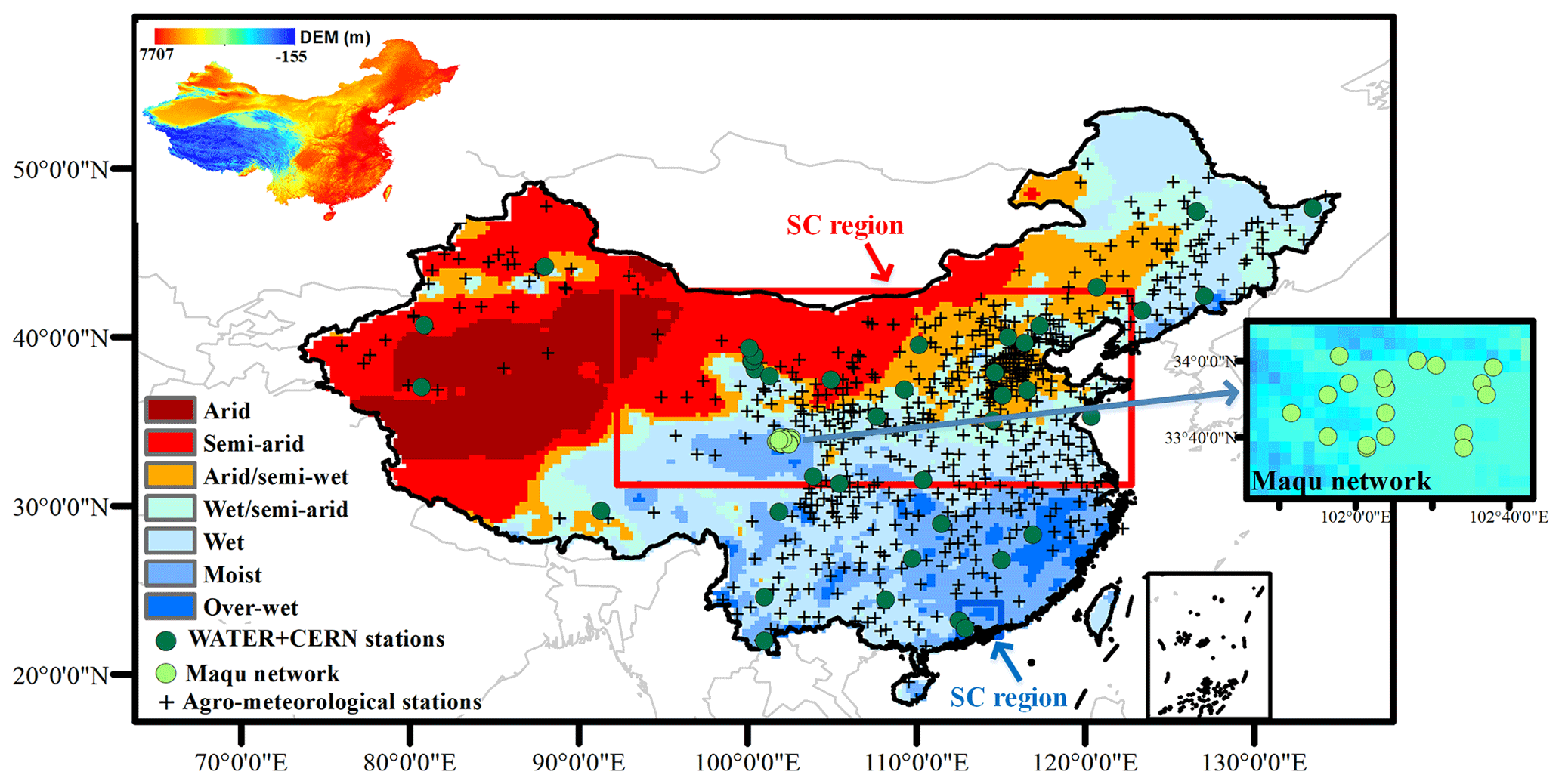
Figure 1 Study region and the selected in situ soil moisture sites. The figure in the upper-left corner shows the digital elevation model (DEM) information. The detailed distribution of dense in situ measurements in the Maqu network is shown in the figure on the far right. Two regional areas for uncertainty analysis (i.e., northern China, NC, and southern China, SC) are bordered by the rectangles.

3 Materials and methods

The object of this study was to reconstruct CCI SM data gaps to produce spatially continuous data records. The basic principle of the proposed gap-filling approach is to efficiently determine the correlation between SM records and the corresponding explanatory variables, which can be expressed as follows:

$$\begin{array}{}\text{(1)}& {\displaystyle }\mathrm{SM}=f\left({\mathit{V}}_{\mathrm{1}},{\mathit{V}}_{\mathrm{2}},{\mathit{V}}_{\mathrm{3}}\mathrm{\dots }{\mathit{V}}_k\right)+\mathit{\epsilon },\text{(2)}& {\displaystyle }{\mathit{V}}_i\in R^{N,T},\end{array}$$

where SM is the soil moisture, V_i are the corresponding explanatory vectors, and k is the number of input variables. V_i can be a vector, and the sample number is determined in the spatial domain (N) and temporal domain (T). f is one function that can be either linear or nonlinear. ε represents the model residual. In a machine learning ensemble, f represents a black box model that does not have one specific form.

The proposed methodology involves three core steps: (i) using a regression subset selection approach and a variable correction procedure to filter explanatory variables from the satellite observations and model-driven knowledge and to correct the systematic variable bias between them (Fig. 2 Part 1, red text); (ii) training a machine learning algorithm to determine the SM–explanatory variable correlation based on the selected optimal parameters and the available pixels identified with a spatiotemporal window search strategy and then applying the established correlation to retrieve the unavailable SM pixels (Fig. 2 Part 2, red text); (iii) conducting geographically weighted regression and Gaussian filtering to calibrate the model-derived residuals (Fig. 2 Part 2, red text).

Figure 2 Schematic of the overall procedure.

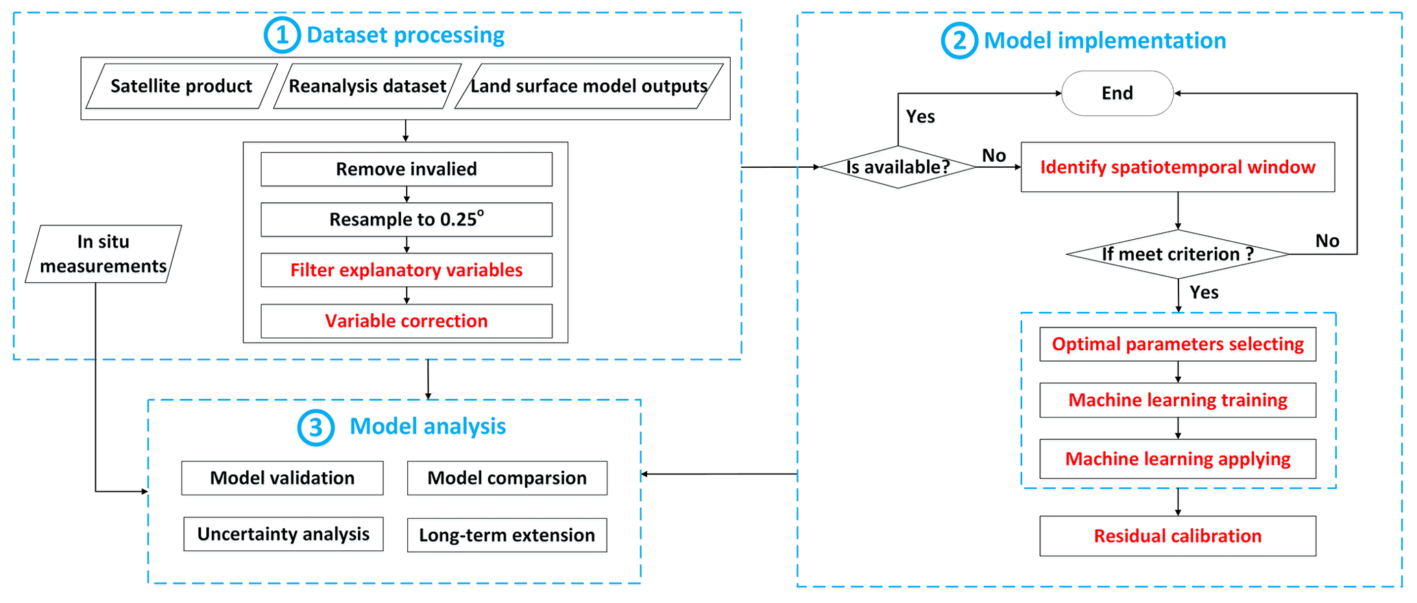
3.1 Dataset processing

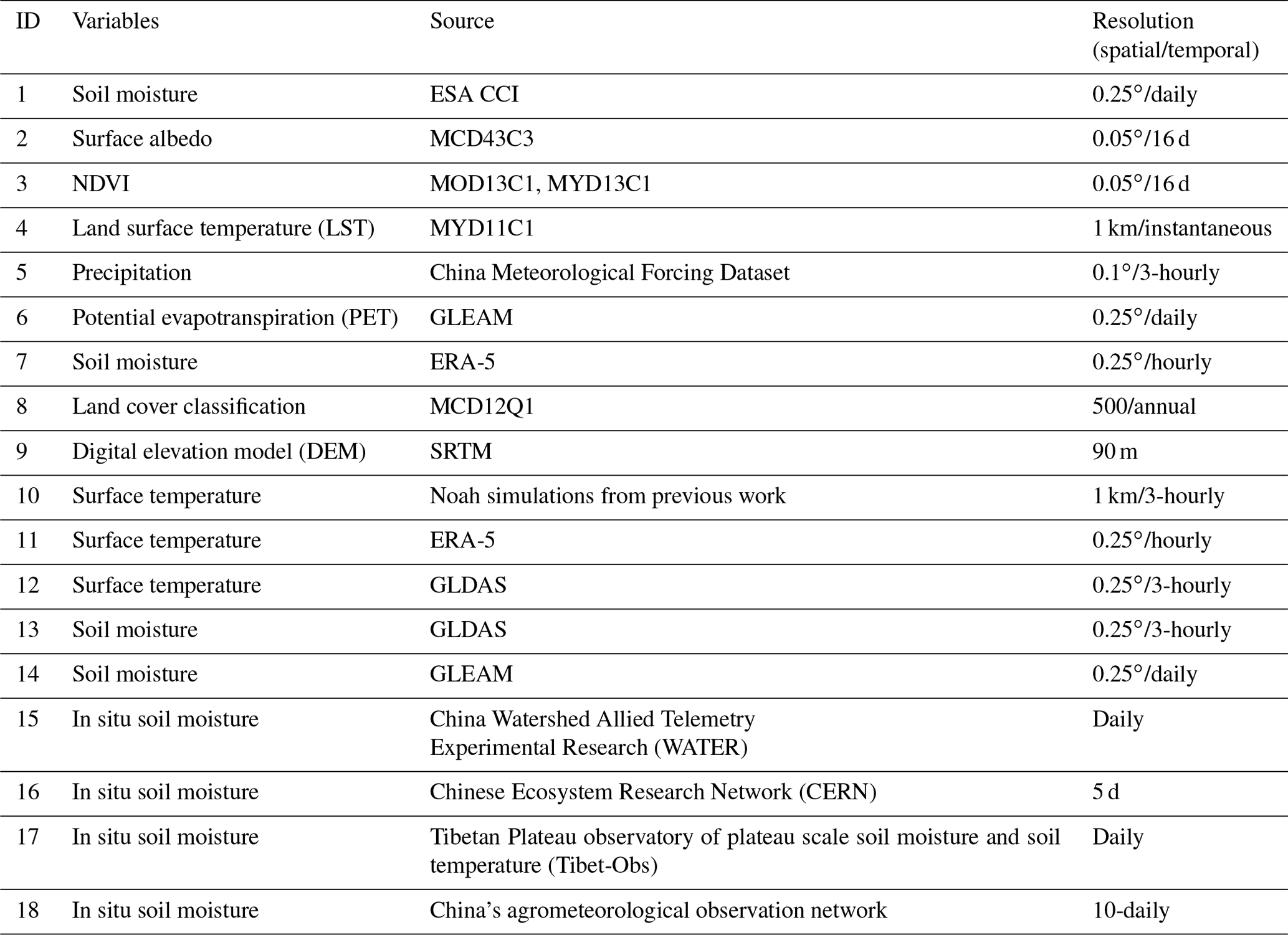
The dataset used includes the satellite product, reanalysis dataset, land surface model outputs, and in situ measurements (Tables 1 and S1). Details about these datasets are described in the following sections.

Table 1 Summary of the dataset used for the proposed model. The other dataset for the preliminary analysis but not the final utilization of the model is exhibited in Table S1 in the Supplement.

3.1.1 Satellite product

The ESA CCI SM dataset is provided by the Climate Change Initiative program of the European Space Agency. This product is primarily composed of three types of daily dataset sources, i.e., active, passive, and active–passive combined microwave products (Dorigo et al., 2017). Despite the wide spatiotemporal coverage of CCI SM, the data gap remains a major challenge that hampers its further application. Here, we select the daily combined microwave products version 4.5 with a spatial resolution of 0.25^∘. The inconsistent data in the CCI combined SM are filtered using the quality flag variable.

A variety of Moderate Resolution Imaging Spectroradiometer (MODIS) products are collected, including the daily LST (MYD11C1), the 16 d composite albedo (MCD43C3) and vegetation indices, i.e., NDVI and EVI, and the 8 d composite leaf area index (LAI) (MCD15A2H). All these datasets are collected at MODIS 6 collection. We calculate the diurnal temperature range (DTR) by subtracting the nighttime LST from the daytime LST. The NDVI and EVI are averagely obtained from the two products: MOD13C1 and MYD13C1. All the selected products are screened out using the quality variables to maintain only the available pixels with good quality. We also collect the 0.05^∘ annual land cover product (MCD12Q1) for quality control of CCI SM.

We use the digital elevation model (DEM) dataset provided by NASA's Shuttle Radar Topography Mission (SRTM) (Van Zyl, 2001) to retrieve several relevant topographic metrics, including slope, aspect, and the topographic position index (TPI) (Guisan et al., 1999). The TPI is calculated by subtracting the focal grid elevation from the mean elevation of the eight surrounding grids. The TPI is potentially correlated better with surface variables such as snow depth and SM in comparison with the DEM (Cristea et al., 2017). Positive (negative) TPI values mean that the target grid is higher (lower) than the average of its surroundings.

Considering the low accuracy of satellite SM for snow-covered pixels, pixels that have both daytime LST lower than 0 ^∘C and albedo higher than 0.3 are removed (Cui et al., 2020). We also remove pixels for which a water body accounts for more than 20 % of the total area. To overcome the spatial resolution differences among the diverse products available, all the datasets are resampled to 0.25^∘ spatial resolution by averaging the pixel values.

3.1.2 Reanalysis dataset and land surface model outputs

We collect the soil moisture data from ERA-5, a global atmospheric reanalysis dataset released by the ECMWF (Balsamo et al., 2015). The data assimilation system used for ERA-5 is the ECMWF Integrated Forecast System (IFS), and the meteorological forcing for retrieving soil moisture is from the ERA atmospheric reanalysis. Here we select the daily-averaged SM from the first soil layer (0–7 cm) to match with satellite CCI SM.

Daily potential evapotranspiration (PET) and surface soil moisture (0–15 cm) are collected from the Global Land-surface Evaporation Amsterdam Methodology (GLEAM) dataset. GLEAM is based on a general land surface model that focuses on soil moisture and evapotranspiration (Miralles et al., 2011). PET in GLEAM is calculated with the Priestley–Taylor formula based on multiple reanalysis datasets, while the soil moisture is calculated with a soil-water module based on the water cycle balance.

Four meteorological variables, i.e., precipitation, air temperature, solar radiation, and wind, are obtained from the China Meteorological Forcing Dataset. This dataset is generated through fusion of in situ station data, remote sensing products, and reanalysis datasets (He et al., 2020). Considering the lag effect of precipitation on surface water dynamics, we use the 5 d antecedent precipitation (AP) to replace the daily precipitation (Wei et al., 2020).

Three surface temperature sources are additionally collected for uncertainty analysis. Two sources are collected from the ERA-5 and GLDAS ensemble models. Considering the model uncertainties caused by regional surface characteristics and climatic conditions, we simulate surface temperature and surface SM (0–10 cm) by implementing a Noah model that is forced with meteorological variables from the Chinese regional ground meteorological dataset and the surface condition parameters from MODIS. This dataset was previously used in our work (Liu et al., 2020a, 2021b).

3.1.3 In situ measurements

A variety of spatially sparse in situ soil moisture measurements is collected to evaluate the accuracy of gap-filled SM. We collect in situ soil moisture observations at 39 sites obtained from the China Watershed Allied Telemetry Experimental Research (WATER) project and the Chinese Ecosystem Research Network (CERN). These validation stations are set up in a relatively large homogeneous area dominated by vegetation covers (cropland, woodland, and grassland) or desert lands. In addition, 657 in situ soil moisture measurements covered by cropland are collected from the Chinese agrometeorological and ecological observation network.

We also collect the dense in situ measurements at the Maqu soil moisture monitoring network. The Maqu network (33^∘30^′–34^∘15^′ N, 101^∘38^′–102^∘45^′ E) is located on the northeastern border of the Tibetan Plateau (Fig. 1) (Dente et al., 2012). In this network, 20 sites are distributed over a uniform grassland cover located in the large valley of the Yellow River. The Maqu network has demonstrated capability in monitoring the spatial and temporal SM variability with high accuracy (Su et al., 2013; Wei et al., 2019). The locations and detailed information of all available sites are displayed in Fig. 1 and Table S2.

3.1.4 Filter explanatory variables

Explanatory variables related to atmospheric, geophysical, ecological, and hydrological variables are conducive to capturing SM variability. The significance percentage produced by the regression subset selection model (Fu et al., 2019; Liu et al., 2021a) is employed to measure the impacting probability of the explanatory variables, where a high significance percentage indicates capability in depicting SM (details in Sect. S1 in the Supplement). We conducted the subset selection model analysis based on a dataset from 2005 to 2015, and 15 variables were selected as input parameters, including 7 surface environmental variables, i.e., albedo, NDVI, EVI, LAI, DTR, PET, and ERA SM, 3 elevation variables, i.e., TPI, aspect, and slope, and 3 climatic variables, i.e., AP, air temperature, wind, and two geographical factors, i.e., latitude and longitude. All the variables are available from datasets at the continental scale. Gaps present in these variables were not considered further to avoid introducing additional errors.

As illustrated in Fig. 3a, albedo, NDVI, EVI, LAI, DTR, AP, PET, ERA SM, TPI, and air temperature have the highest significance percentage in terms of correlation with CCI SM. We excluded aspect, slope, wind, latitude, and longitude owing to their low correlations with SM. The EVI, NDVI, and air temperature were also not considered in further application because the EVI and LAI are closely correlated with NDVI, and air temperature is strongly correlated with DTR. All the selected covariates are physically meaningful in depicting SM. Specifically, the atmospheric variables (i.e., precipitation and PET) are suitable for capturing the temporal dynamics of SM, and the topographic variables are included both to depict the orographic effects and to recapture the spatial pattern of SM. DTR exhibits correlation with SM owing to its capacity to take account of land–atmosphere coupling. ERA SM was also included to reproduce satellite SM.

To verify the results based on the regression subset selection model, we employed the permutation feature importance to measure the relative importance of each predictor variable. Consistent patterns between the significance percentage and permutation importance further indicate the feasibility of the selected variables in modeling SM. Additionally, because these variables are derived from optical remote sensing, reanalysis datasets, and land surface model products, they have potential for extension to large regions owing to their high availability (Fig. 3b).

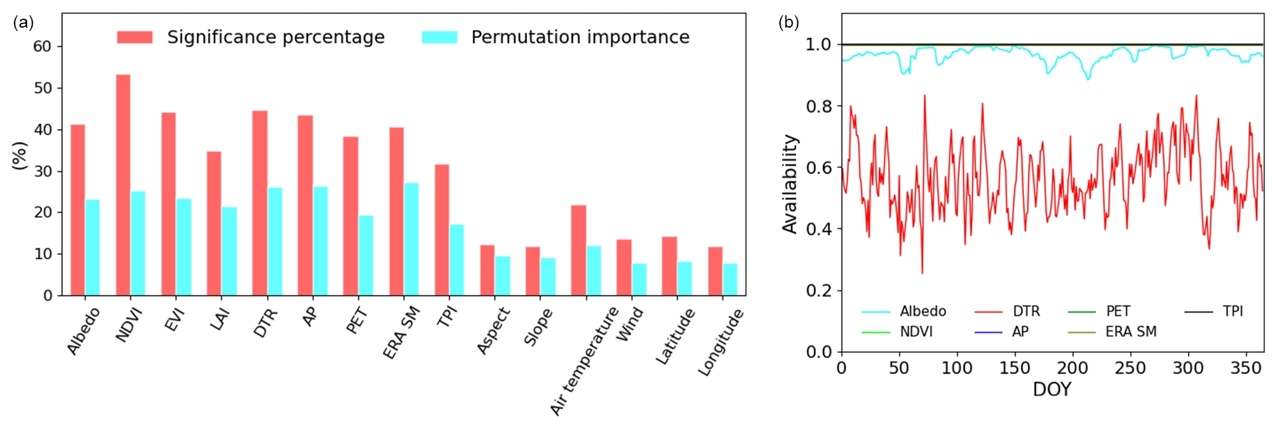
Figure 3 Correlation and availability of the dataset used. (a) Significance percentage and permutation importance of the selected variables in correlation with CCI SM. (b) Availability of the selected variables.

3.1.5 Variable correction

Systematic biases are unavoidable in reanalysis datasets and land surface model outputs, and these biases can be propagated in dynamic modeling. Accordingly, bias correction is required prior to the gap-filling procedure to ensure a consistent simulated output. Specifically, to make the modeled values (i.e., ERA SM) comparable with the satellite observations (i.e., ESA CCI SM), we used a correction procedure that primarily combines a variance scaling algorithm and a linear scaling algorithm (Long et al., 2020; Zhang et al., 2021c). The used procedure can be illustrated with the following equations:

$$\begin{array}{}\text{(3)}& \left\{\begin{array}{l}{\mathrm{SM}}_{\mathrm{c}\mathrm{1}}={\mathrm{SM}}_{\mathrm{ERA}}\left(t_{\mathrm{av}}\right)-\mathit{\mu }\left({\mathrm{SM}}_{\mathrm{ERA}}\left(t_{\mathrm{av}}\right)\right)+\\ \mathit{\mu }\left({\mathrm{SM}}_{\mathrm{ESA}}\left(t_{\mathrm{av}}\right)\right),\\ {\mathrm{SM}}_{\mathrm{c}}=\mathit{\mu }\left({\mathrm{SM}}_{\mathrm{c}\mathrm{1}}\right)+({\mathrm{SM}}_{\mathrm{c}\mathrm{1}}-\mathit{\mu }\left({\mathrm{SM}}_{\mathrm{c}\mathrm{1}}\right))\\ \times \mathit{\sigma }\left({\mathrm{SM}}_{\mathrm{ESA}}\left(t_{\mathrm{av}}\right)\right)/\mathit{\sigma }\left({\mathrm{SM}}_{\mathrm{c}\mathrm{1}}-\mathit{\mu }\left({\mathrm{SM}}_{\mathrm{c}\mathrm{1}}\right)\right),\end{array}\right.\end{array}$$

where SM_ERA is the raw ERA SM time series of the target grid pixel, t_av is the time series in which pixels of the object grid are available, SM_ESA is the ESA SM of the grid, and μ and σ are the mean value and the standard deviation, respectively. SM_c is the corrected ERA SM that is assumed to have a spatial pattern (i.e., consistent means and standard deviations) with the CCI SM. In our study, a dataset comprising time series from 2005 to 2015 was used to conduct the correction procedure to guarantee sufficient samples. Examples illustrating the performance of the ERA SM correction can be found in Fig. S1. Despite being conducted on SM, this calibration procedure could be applied to other parameters (e.g., DTR) when replaced with numerical model outputs.

3.2 Model implementation

3.2.1 Machine learning regression

Despite being easy to implement and requiring fewer computational resources, traditional regression-based methods such as generalized linear models and multivariate regression splines generally insufficiently consider the probability density functions in assessing model performance. Machine learning approaches could be much more flexible than conventional parametric models owing to their ability to handle nonlinear relationships and complex interactions. Among the various machine learning models, the random forest (RF) algorithm, acting as an enhanced decision tree model, is an effective and powerful tool in interpreting Earth variables (Belgiu and Dragut, 2016). As illustrated in Fig. 4a, RF is a hierarchical tree diagram that is based on a nonparametric strategy and has the capacity to add a variety of parameter layers to the model (Breiman, 2001). This decision tree model is composed of many nodes and edges within each tree structure, mainly including two types of nodes: split nodes and leaf nodes. The split node is related to a test function that is employed to split the input data, whereas the leaf node is associated with the final decision. Unlike the standard decision tree model that relied on the whole dataset, RF trains each tree on bootstrap resamples. This model only considers the randomly selected variables rather than the total variables. By this means, the outcome is decided by a majority voting or averaging strategy.

In this study, the RF model is implemented using the “RF Regressor” function from the Python library (Shahriari et al., 2016). Specifically, the built-in functions are used to assess the importance of each covariate by using the out-of-bag samples. We use the “Bayesian Optimization” module (http://rmcantin.github.io/bayesopt/html/bopttheory.html, last access: 20 August 2021) to select the best hyperparameters in driving the RF algorithm. Four critical parameters deciding the RF algorithm include the number of trees (n_estimators), the maximum tree depth (max_depth), the minimum number of samples for splitting an internal node (min_samples_split), and the number of features (max_features). For each specific climate region, the Bayesian optimization process is carried out within 20 iterations to optimal parameters. This procedure is implemented by using the dataset of 2003–2008 as the cross-validation window. Optimal parameters in the seven climate regions are listed in Table S3.

3.2.2 Identify the spatiotemporal window

One critical issue related to the machine learning model is how to efficiently explore the informative covariates. Here, we use a spatiotemporal strategy to capture the spatial and temporal SM and the related covariate dynamics. Our strategy primarily relies on the available pixels within a regional subset, thereby allowing more pixels of interest to participate in the regression. Figure 4b provides the diagram of the spatiotemporal window search strategy.

An adaptive strategy is employed to determine the optimal spatiotemporal window size. Two critical variables are adopted to identify the window size, i.e., the size of the spatial window (sw) and the number of temporal days (nd). To find the optimal sw and nd, we continually increase the value of sw and nd from the initial values until the samples participating in regression meet the criterion; i.e., the number of available pixels within the searched window should be no less than 8 times the participating explanatory variables (i.e., seven) (Svetnik et al., 2003; Liu et al., 2020a). Here an initial sw is set to 5 and an initial nd is set to 1. Considering that a fraction of gaps occurs in the satellite dataset (e.g., LST and albedo) and the optimal window may not exist, the maximum values of sw and nd are introduced to terminate this process. A sensitivity analysis is conducted with the independent dataset to select the two maximum values. Specifically, we conduct a cross-validation during 2003–2008 to evaluate the accuracy of the gap-filling model. The increasing maximum nd from 1 to 7 with intervals of length 1 is tested, and the maximum sw is tested from 4 to 10 with intervals of length 1. The values that yield the lowest RMSE (Fig. 4c) are selected, and finally, we set the maximum sw to 7 and the maximum nd to 4. Note that we also conduct a sensitivity analysis for each climate region and find no substantial differences in the resulting optimal values of two parameters among the seven climate regions. This is probably because this sensitivity analysis is more reliant on model structure rather than sample characteristics.

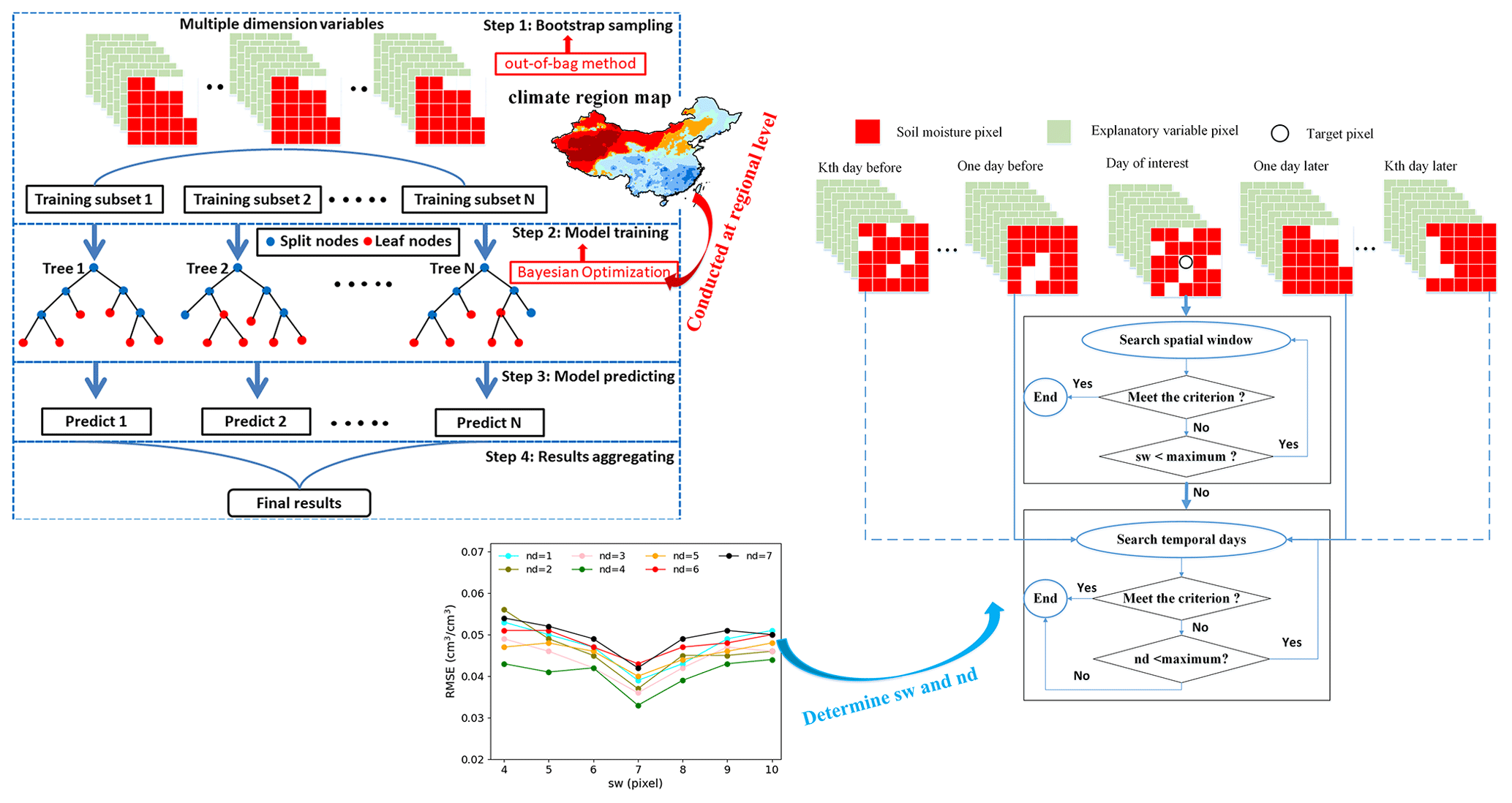
Figure 4 (a) Diagram of the random forest model implemented for a multidimensional dataset. (b) Diagram of the spatiotemporal window determination strategy for random forest regression. (c) Results of the sensitivity analysis regarding two maximum values, i.e., the size of the spatial window (sw) and the number of temporal days (nd), for terminating the searching process.

3.2.3 Residual calibration

Considering that the machine learning model might not fully account for the variability in SM, the original reconstruction needs to be calibrated, which can potentially remove the bias resulting from neglected variables such as those that are excluded for model establishment (Zhu et al., 2012; Liu et al., 2020a). In practice, we add the interpolated model residuals to the original reconstructions. The geographically weighted regression (GWR) model, which is an extension of the traditional linear regression model (Li et al., 2017), is applied to interpolate the RF-derived residuals. This procedure is based on the samples within the searched window for each target pixel. The model residual (ε_j) derived from Eq. (1) can be described using the explanatory variables as follows:

$$\begin{array}{}\text{(4)}& {\mathit{\epsilon }}_j={\mathit{\beta }}_{\mathrm{0}}\left(u_j,v_j\right)+{\sum }_{i=\mathrm{0}}^k{\mathit{\beta }}_i\left(u_j,v_j\right)X_{ij},\end{array}$$

where β₀(u_j,v_j) and β_i(u_j,v_j) are the regression coefficients estimated at the jth pixel, and (u_j,v_j) are the coordinates. The regression coefficients can be estimated using the observations within the self-adaptive searched window as follows:

$$\begin{array}{}\text{(5)}& \left\{\begin{array}{l}\widehat{\mathit{\beta }}\left(u_j,v_j\right)=\left(X^T\right(W\left(u_j,v_j\right))X{)}^{-\mathrm{1}}{X}^{T}W\left(u_j,v_j\right)Y,\\ w_{ij}=[\mathrm{1}-(d_{ij}/b{)}^{\mathrm{2}}{]}^{\mathrm{2}},\end{array}\right.\end{array}$$

where $\widehat{\mathit{\beta }}\left(u_j,v_j\right)$ is the coefficient matrix composed of coefficients from each explanatory variable, and X and Y are the explanatory variable matrix and the dependent variable (i.e., SM) vector, respectively. Here latitude, longitude, and the seven explanatory variables selected are used to implement the GWR model. W(u_j,v_j) is the weight matrix composed of w_ij, d_ij is the Euclidean distance between the observation ith and jth points, and a and b are the window radii.

Before adding to the original reconstruction, the GWR-interpolated residual is further smoothed with a normalized k×k Gaussian filter with a standard deviation of σ. This procedure can remove the grid-like artifacts that extensively exist in statistical model outcomes. Based on the optimization procedure (Sismanidis et al., 2021; Liu et al., 2019), we set k=5 and σ=1.5.

3.3 Model analysis

3.3.1 Model validation

Model validation was conducted using data from 2009 when a sufficient number of ground measurements was collected. The top layer SM measurements from the in situ stations were first used to evaluate the accuracy of the reconstructed results. Considering the scale mismatch between the sparse distribution of in situ stations and the CCI SM product (∼25 km), we used the Disaggregation based on Physical And Theoretical scale Change (DISPATCH) model (Merlin et al., 2012) to disaggregate the 0.25^∘ reconstructions to 1 km resolution. Detailed descriptions regarding this disaggregation method can be found in Sect. S2 in the Supplement.

Evaluating the gap-filled SM with in situ measurements can produce biases that can be caused by scale mismatching and disaggregation model performance. To account for this, holdout cross-validation with 10 replicates was performed in 2009 to evaluate the model accuracy. For each replicate, we randomly held out 10 % of the pixels, that is, manually introducing gaps for these pixels, and trained the model with the remaining 90 % of the dataset. Specifically, the pixels during all the periods were first rearranged into a time series, and then 10 % of them were dropped in each replicate. After the gap-filled SM series of holdout pixels were reconstructed from the training set, they were validated against the original SM.

To reveal the physical plausibility of gap-filled SM, we paid particular attention to the evaluation of gap-filling SM under extremely dry conditions. Extreme drought is defined based on meteorological conditions, that is, the Palmer Drought Severity Index (PDSI) of less than −2 over 8 consecutive months or longer (Fig. S2).

The statistics used for the model accuracy assessment include the coefficient of determination (R²), the root mean square error (RMSE), the mean absolute error (MAE), the average error bias (BIAS), and the unbiased RMSE (ubRMSE). In addition, Nash–Sutcliffe efficiency (NSE) is used to measure the overall performance of the proposed model. All these metrics have been extensively used for evaluating satellite SM.

3.3.2 Model comparison

The proposed method was compared against four extensively used models that adopt the same explanatory variables and spatiotemporal window search strategy. The first one is the conventional multiple linear regression (MLR) approach. Three typical machine learning approaches, i.e., extreme gradient boost (XGB), support vector machine (SVM), and artificial neural network (ANN), are also used for comparison. Detailed descriptions of the four available models can be found in Sect. S3.

3.3.3 Uncertainty analysis

Considering the criticality of explanatory variables in simulating SM, uncertainty analyses regarding these selected variables were conducted. We first investigated the accuracy of the reconstruction model that excludes one participating variable. Given the critical importance of satellite-derived DTR and the severe issues of missing data in satellite-observed LST products, we further investigated the substitution performance of other surface temperature sources in reconstructing SM, i.e., Noah, ERA, and GLDAS. This analysis was conducted by focusing on two regions (in Fig. 1) that have sufficient data sources to support our experiments (Liu et al., 2020a, 2021b): one region is in northern China covering mostly arid and semi-arid areas, while the other region is in southern China covering mostly wet areas.

Since the reanalysis SM is a vital input in our approach, we also compare it with the other two products to evaluate the feasibility of ERA data in reconstructing CCI SM. GLEAM and Noah surface SM are, respectively, employed to replace the ERA SM, while the other explanatory variables keep the rest the same.

3.3.4 Long-term extension

The available dataset forcing for our model has a long record, indicating potential for modeling long-term SM products. To verify this, the proposed gap-filling method was further extended to the long-term ECA CCI SM databases of 2005–2015. We also investigated the trend of the SM series during this period, which was obtained via Sen's slope and Mann–Kendall significance analysis (Li et al., 2021a, c). The trends from the reconstructed SM series were also compared with those from the original CCI SM, which were evaluated against in situ measurements.

4 Results and discussion

4.1 Spatiotemporal patterns

The spatiotemporal pattern of the original daily CCI SM and the corresponding gap-filled dataset in 2009 is first checked. As shown in Fig. 5a (and Fig. S3), a considerably large gap occurs in the original CCI SM, and this gap problem is greater in winter. We reconstruct the contaminated SM pixels using the spatiotemporal RF model. Most of the contaminated pixels (more than 85 %) are reconstructed. Relatively few missing pixels are gap-filled in winter in comparison with other seasons, primarily because of the heavy contamination of clear pixels caused by frequent occurrence of cloud during this period. It means that the learning capacity of the spatiotemporal machine learning method is constrained when encountering limited satellite observations.

Figure 5b shows the box plot of the original versus gap-filled SM on selected days in 2009. Conformity exists between the original and reconstructed SM for most days. A similar pattern in variance and magnitude is also observed for the SM of the monthly average and the selected days, as illustrated in Fig. 5c; that is, a large difference occurs in winter and spring. This can be attributed to the fact that the original CCI SM provides fewer training data from October to May of the following year. Additionally, the distribution of CCI SM is more uneven in this period, which might reduce model performance owing to the limited representation of training samples (Stroud et al., 2001).

In terms of different climate regions, a minor discrepancy is evident between the original and reconstructed SM (Fig. 5d), with a bias in the median SM values of less than 8 %. It means that the reconstructed SM has variation-depicting capacity. Small overestimation occurs in arid regions, which originally had less soil water storage.

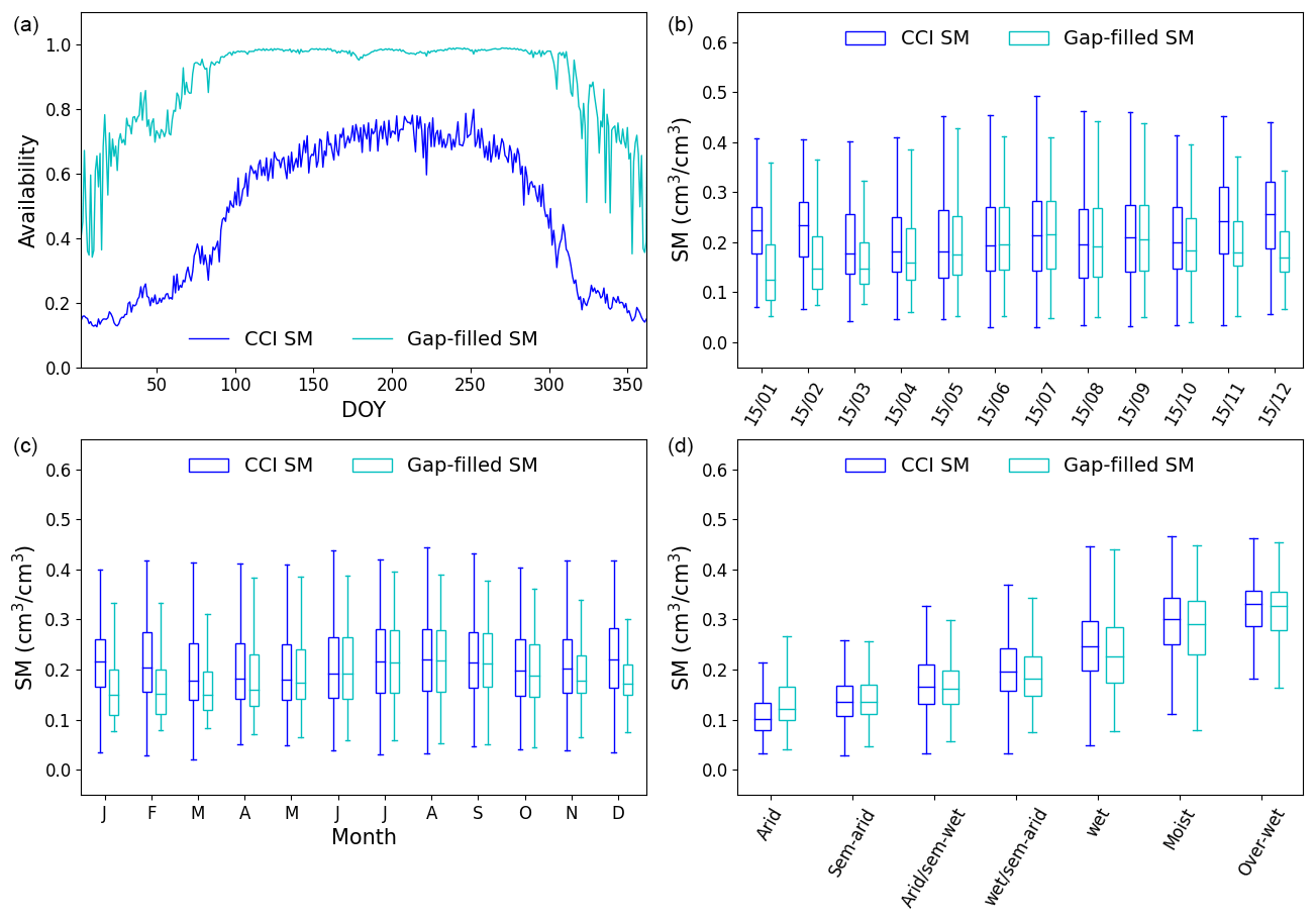
Figure 5 Comparison between the CCI dataset and gap-filled SM in 2009. (a) Plots of the availability of the CCI dataset and gap-filled SM. (b) Box plot of the CCI dataset and gap-filled SM on the selected days. (c) Box plot of the month-average CCI and gap-filled SM. (d) Box plot of raw and gap-filled SM regarding seven climate regions.

Figure 6 exhibits the spatial distributions of the original CCI SM and the reconstructed SM on selected days in 2009. The humid regions are mostly concentrated in southern China adjacent to the coast of the western Pacific, whereas the dry regions are mainly distributed in the northern and western parts of China. A considerable fraction of contaminated pixels is observed on the selected days, and this contamination is severe in the winter season and in mountainous areas and snow-covered regions (e.g., Tibetan Plateau and Mongolian Plateau). Almost all the contaminated pixels from March to October are reconstructed; meanwhile, the proposed model reconstructs the most contaminated pixels for the remaining months. Owing to the additional valid values provided by gap-filled pixels, more spatial variation is depicted in the reconstructed SM images. Missing pixels still occur in the reconstructed SM images, especially in the cold seasons. This is probably related to the fact that the surface temperature, ET, and precipitation are more connected in the warm season through energy balance considerations and atmospheric circulation. Some of these invalid pixels correspond to snow- and water-covered regions that have been removed beforehand. Because missing Earth data are to a large extent not at random, statistical measures of comparative analysis among them tends to produce bias (Bessenbacher et al., 2022b). To account for this, paired histograms of two datasets are compared to explore the value distribution properties. The histograms show that the gap-filled dataset does not impact the SM distribution in warm seasons, that is, in agreement with the CCI dataset. However, this bias cannot fully indicate the improved accuracy of gap-filled SM because the pixels could be missing not at random.

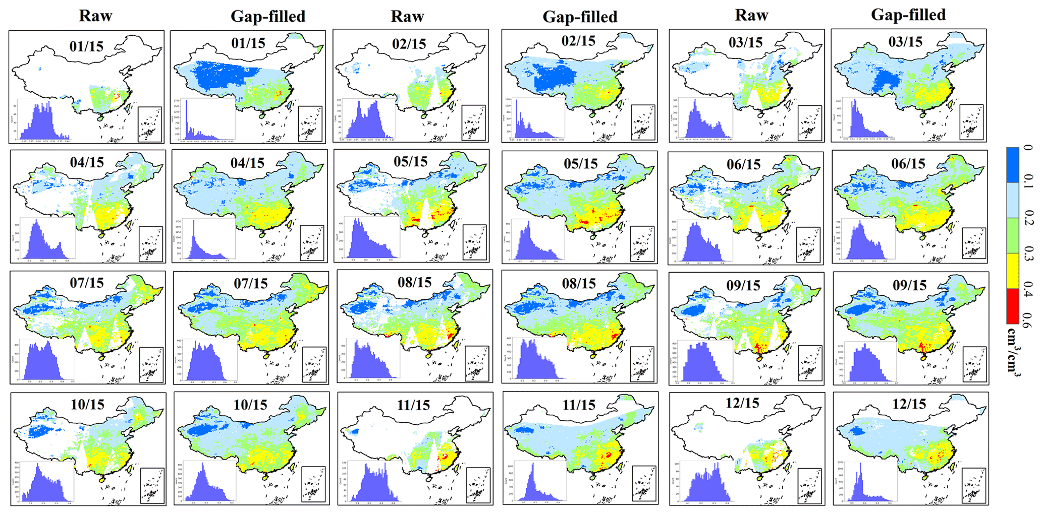
Figure 6 Spatial distributions and histogram of the raw and gap-filled CCI SM on the 15th of each month in 2009.

4.2 Accuracy validation with in situ measurements

The proposed model is first evaluated with sparse in situ measurements from WATER and CERN. As shown in Fig. 7a, agreement is obtained between the 1 km CCI SM-derived values and the in situ measurements, with an R² of 0.8. This accordance is also found between the 1 km reconstructed SM and the in situ measurements (Fig. 7b), with an R² of 0.75. High accuracy is also observed when performing evaluation with in situ measurements from national agrometeorological stations. The R² value between the 1 km CCI SM-derived values and the in situ measurements is 0.81, while the R² value between the 1 km reconstructed SM and the in situ measurements is 0.71 (Fig. 7c and d). Inconsistency evidently remains, and noticeable overestimations are observed in the high range of SM. Additionally, the accuracy of the gap-filling products tends to be diminished by drought conditions, but this impact is limited.

We further validate the reconstructed results with the dense in situ measurements from the Maqu network. The RMSE and MAE values are 0.11 and 0.09 cm³ cm⁻³ (Fig. 7e), respectively, for the 1 km CCI SM-derived values, and 0.12 and 0.09 cm³ cm⁻³ (Fig. 7f), respectively, for the 1 km reconstructed SM. It means that reasonable agreement is obtained for both the CCI SM product and the gap-filled SM; however, poor performance is found in the range of low values, mostly because of the extreme conditions and the fewer samples available for model regression.

The time series of average 0.25^∘ CCI SM values and reconstructed SM over the dense grid are compared with the dense in situ observations. Both the original and reconstructed SM match well with the in situ series, with NSE values of 0.83 and 0.85, respectively. The reconstructed SM (Fig. 7g) mostly describes the temporal dynamics of in situ measurements, that is, sufficiently capturing seasonal and daily variability. In addition, the rainfall events impacting the surface dynamics are observed to be well depicted in the SM temporal variations. The reconstructed SM appears to have inherited the merits of stability between April and November from the CCI SM, i.e., having comparable values during this period.

4.3 Accuracy validation with cross-validation analysis

Cross-validation analysis is further performed with 2009 data to evaluate model performance. The obtained metrics (Fig. 8a) illustrate reasonable coincidence between the reconstructed and original CCI SM, with a median R² range of 0.51 to 0.63. Better accuracy of gap-filled SM in comparison to original CCI SM is also demonstrated by the metrics of RMSE, MAE, and ubRMSE. In particular, the median of BIAS is less than 0.01 cm³ cm⁻³. Comparatively, better accuracy is achieved in the growth seasons (March–October), which can be attributed to the fact that the critical environmental factors, such as NDVI, DTR, and ERA SM, are more related to satellite-derived SM during the season of vegetation growth (Chen et al., 2014; Otkin et al., 2016).

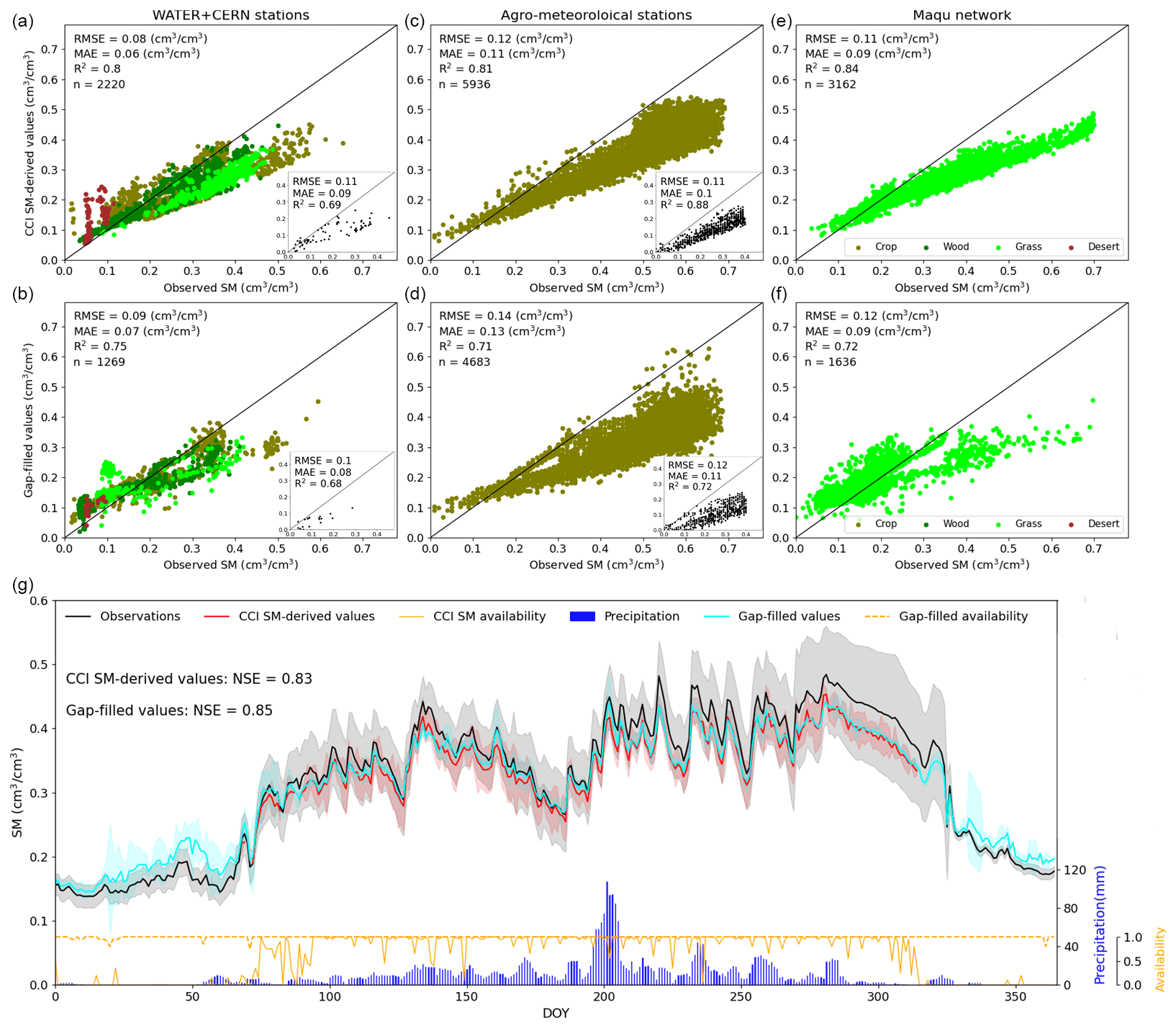
Figure 7 Evaluations of model results. Panels (a), (c), and (e) are the scatter plots of 1 km CCI SM-derived values against field measures regarding WATER/CERN, agrometeorological stations, and the Maqu network, respectively, and panels (b), (d), and (f) are the scatter plots of 1 km gap-filled SM-derived values against field measures. The subfigures in the upper corners of panels (a)–(d) are the scatter plots under extremely dry conditions. Panel (g) is the time series of average CCI SM-derived values against site measures in the Maqu region. The shaded area in panel (g) denotes ±1 standard error.

Figure 8b shows the accuracy metrics for different climate regions. A pattern similar to that of the monthly means is observed; that is, acceptable accuracy occurs in most regions. No significant differences in median R² and BIAS are evident between the reconstructed SM of each climate region, with the bias between the maximum and minimum median R² and BIAS values being less than 0.09 and 0.003 cm³ cm⁻³, respectively. The metrics indicate relatively poor performance in wet regions with high specific heat capacity and low albedo. The lower amounts and high thermal entropy of the available variables (i.e., LST and albedo) in these areas can affect model capacity and stability (Wang et al., 2005). Notably, despite the relatively high RMSE, MAE, and ubRMSE values in the humid region, the R² value is very high (Fig. 10), which might be attributable to the high SM variability in these areas. The accuracy is lower over the regions that experience drought due to perturbations of the soil water content but without noticeably poor performances.

The spatial distributions of the accuracy metrics in Fig. 9 further illustrate the accuracy of the proposed gap-filling model. Discrepancies are observed in some regions, but they rarely exceed 0.09 cm³ cm⁻³ in absolute value. Spatially, the distribution of reconstructed SM follows a geographic gradient. The relatively low accuracies occur in areas of complex terrain in western China. For these regions, complex atmospheric conditions caused by high elevations tend to affect the simulation of surface parameters. Complex topography can result in a complicated directional anisotropy, bringing great uncertainty in modeling surface energy and water cycles (Hu et al., 2016).

The gap-filling model could be sensitive to irrigation and drought owing to the induced inhibition and water stress of vegetation. On the one hand, lower accuracy is found as expected over a considerable fraction of irrigated cropland (e.g., northern China), which can be partly attributed to the human irrigation drain. On the other hand, focused analyses illustrate the consistency of the gap-filling SM with the in situ measurements and the original SM under extremely dry conditions (Fig. S4), illustrating the physical plausibility of the gap-filled values for specific application.

Figure 8 Accuracy metrics of 10 cross-validations for R², RMSE, MAE, BIAS, ubRMSE, and NSE: panel (a) is averagely obtained on a monthly basis, and panel (b) is averagely obtained for each climate region and for the drought grids.

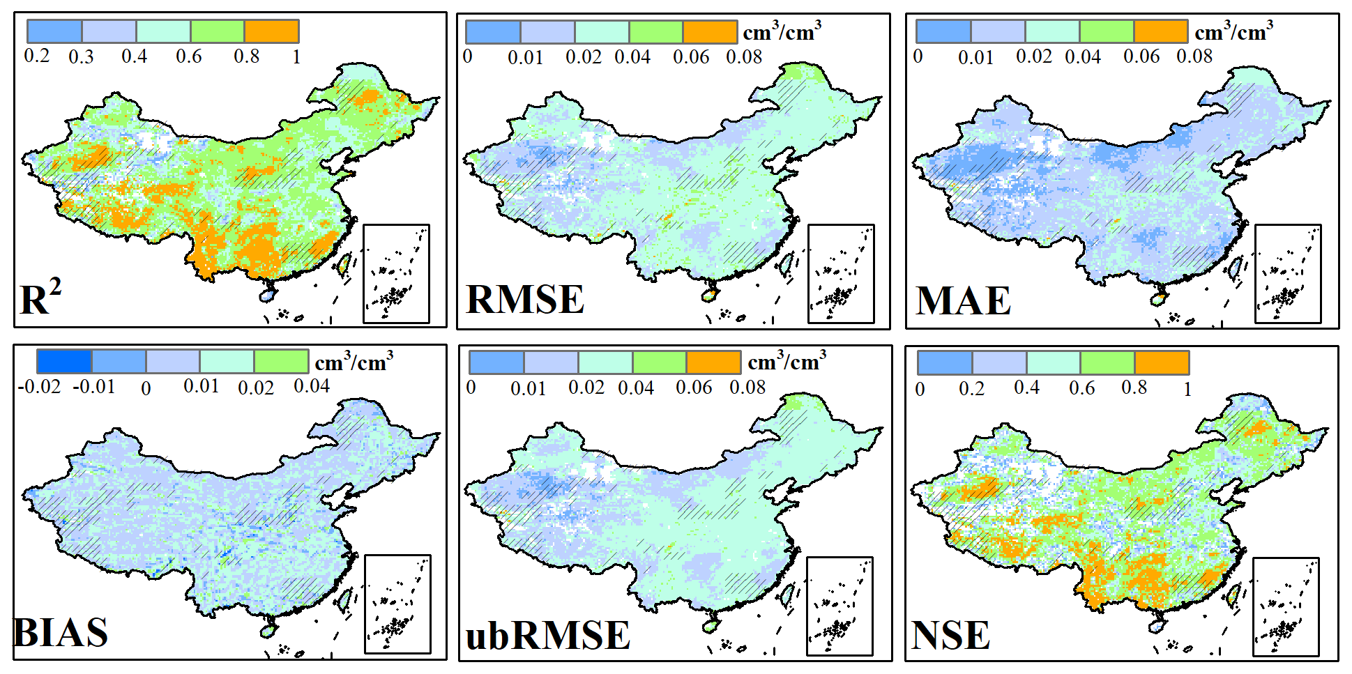
Figure 9 Spatial distributions of accuracy metrics of 10 cross-validations in 2009 for R², RMSE, MAE, BIAS, ubRMSE, and NSE. The slash represents the regions impacted by drought.

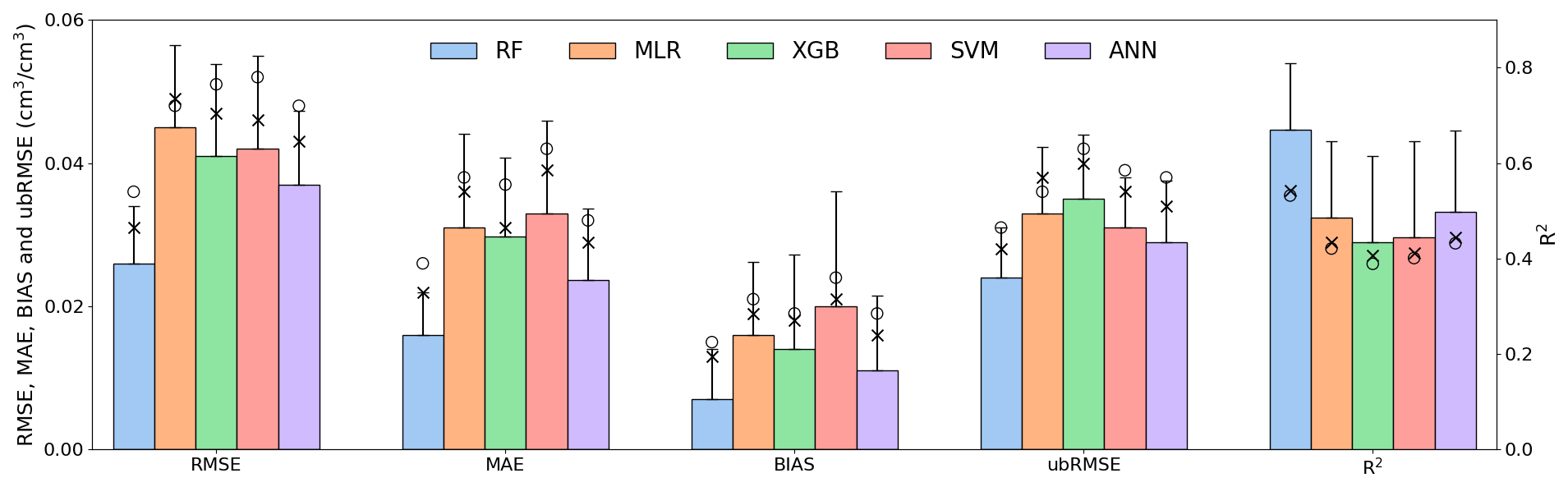
Figure 10 Comparison RF-based model with other models (i.e., MLR, XGB, SVM, and ANN). Error bars denote 1σ errors. The “x” symbol represents the accuracy metrics of models excluding the residual calibration, and the “o” symbol represents the accuracy metrics of the models that use the global regression rather than the regional regression based on the spatiotemporal window searching strategy.

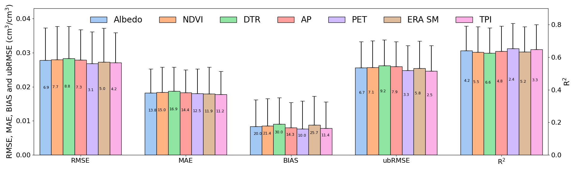
Figure 11 Accuracy of the models removing one variable, i.e., using the other six variables in model regression. Error bars denote 1σ errors. The text denotes the relative percentage of the decreased accuracy of the model with six variables (i.e., excluding one) in comparison with that of a model with seven variables.

4.4 Comparison analysis

The proposed method is further compared against four extensively used models, and the accuracy metrics of the five models are shown in Fig. 10. Generally, the MLR, XGB, SVM, and ANN, accompanying the RF, could potentially reconstruct the missing CCI SM pixels, indicating the stable suitability of these models and the feasibility of available variables. Moreover, the RF model demonstrates prominent performance among all the tested models, further demonstrating its capacity for reconstructing SM when integrating an effective dataset source and mining method. Our results are consistent with earlier studies that illustrated the robustness of the RF approach in simulating satellite parameters (Karbalaye Ghorbanpour et al., 2021; Zhao et al., 2018). This is attributed to the capacity of the RF method to cope with sparse samples, in addition to the fact that the RF does not assume a specific functional or geometric form of the model. We also check the accuracy of the models excluding the residual calibration procedure, which is an essential component of the proposed model. Results (in Fig. 10) demonstrate that accuracies are lowered by ∼9 % when removing the residual calibration, underscoring the importance of residual modulation in improving SM reconstruction. Moreover, better performance brought by the spatiotemporal domain strategy is also exhibited when compared with the global regression. Quantitatively, the spatiotemporal domains can improve the accuracy by ∼19 % in forcing the RF regression. Overall, these analyses indicate the feasibility of the proposed model by integrating the modules of the residual calibration and the spatiotemporal domain strategy.

4.5 Uncertainty analysis

We investigate the accuracy of the reconstruction model that excludes one participating variable. As illustrated in Fig. 11a, the performance of the model with six variables (i.e., excluding one) is relatively low when compared with that of a model with seven variables. The strategy of removing one variable can lower the accuracy by 2.2 %–6.4 % in terms of R² and by 10 %–30 % in terms of BIAS. This diminished performance is plausible because SM is heavily related to all the selected variables. Specifically, variability in land surface characteristics (NDVI and albedo) and atmospheric conditions (i.e., precipitation and PET) can impact SM variability. This is plausible because satellite SM retrievals represent the signals from the upper soil layer, which is directly exposed to the land and the atmosphere. Meanwhile, additional covariates mean an increase in the number of samples participating in the regression model, therefore potentially resulting in improvement in the overall accuracy. We observe that the lowest accuracy occurs when DTR is excluded, underscoring the vital role of DTR in modeling SM.

The importance scores produced by the RF algorithm (Zhao et al., 2019b; Ramoelo et al., 2015) (Fig. S5) also show that all the selected variables substantially impact the CCI SM simulations. Specifically, DTR shows the greatest importance, mainly relating to the fact that temperature variations might influence SM fluctuation. This supports the higher model performance observed in warm seasons, during which PET, albedo, and NDVI exhibit a higher importance score. During this period, heat from the surface can be transferred to the atmosphere via ET and sensible heat conduction, thereby modifying surface SM variations (Amani et al., 2017).

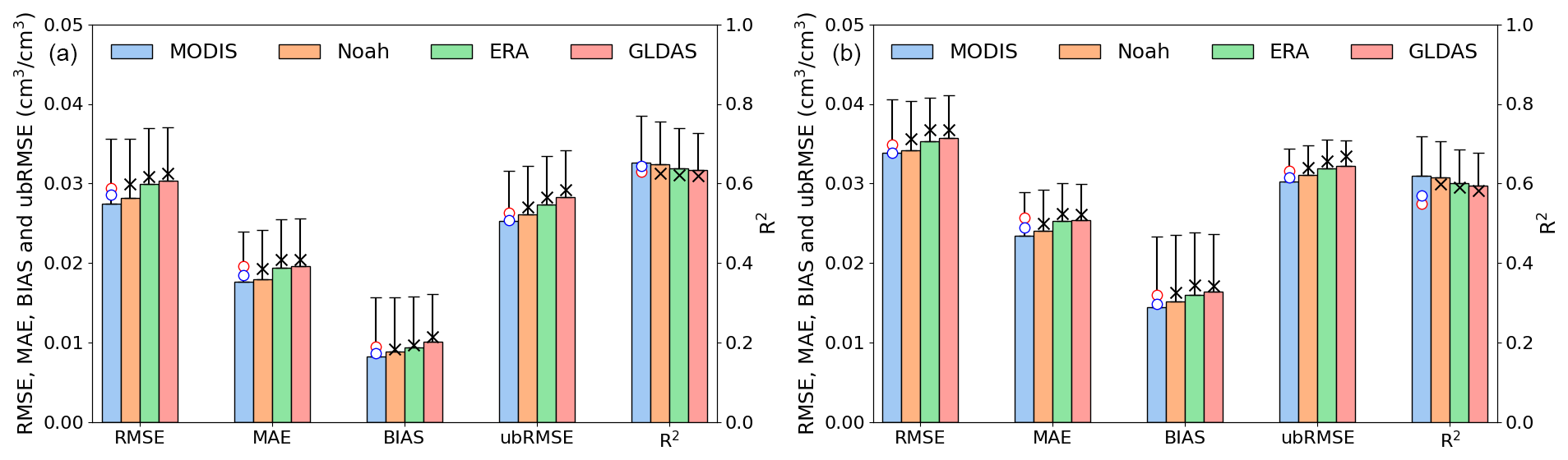
Figure 12 Metrics of models using different DTRs for (a) NC and (b) SC. Error bars denote 1σ errors. The “x” symbol represents the accuracy metrics of the models without the DTR correction procedure. The “o” symbol in red represents the accuracy metrics of the models using GLEAM SM to replace ERA SM, and the “o” symbol in blue represents the accuracy of the models using Noah SM to replace ERA SM.

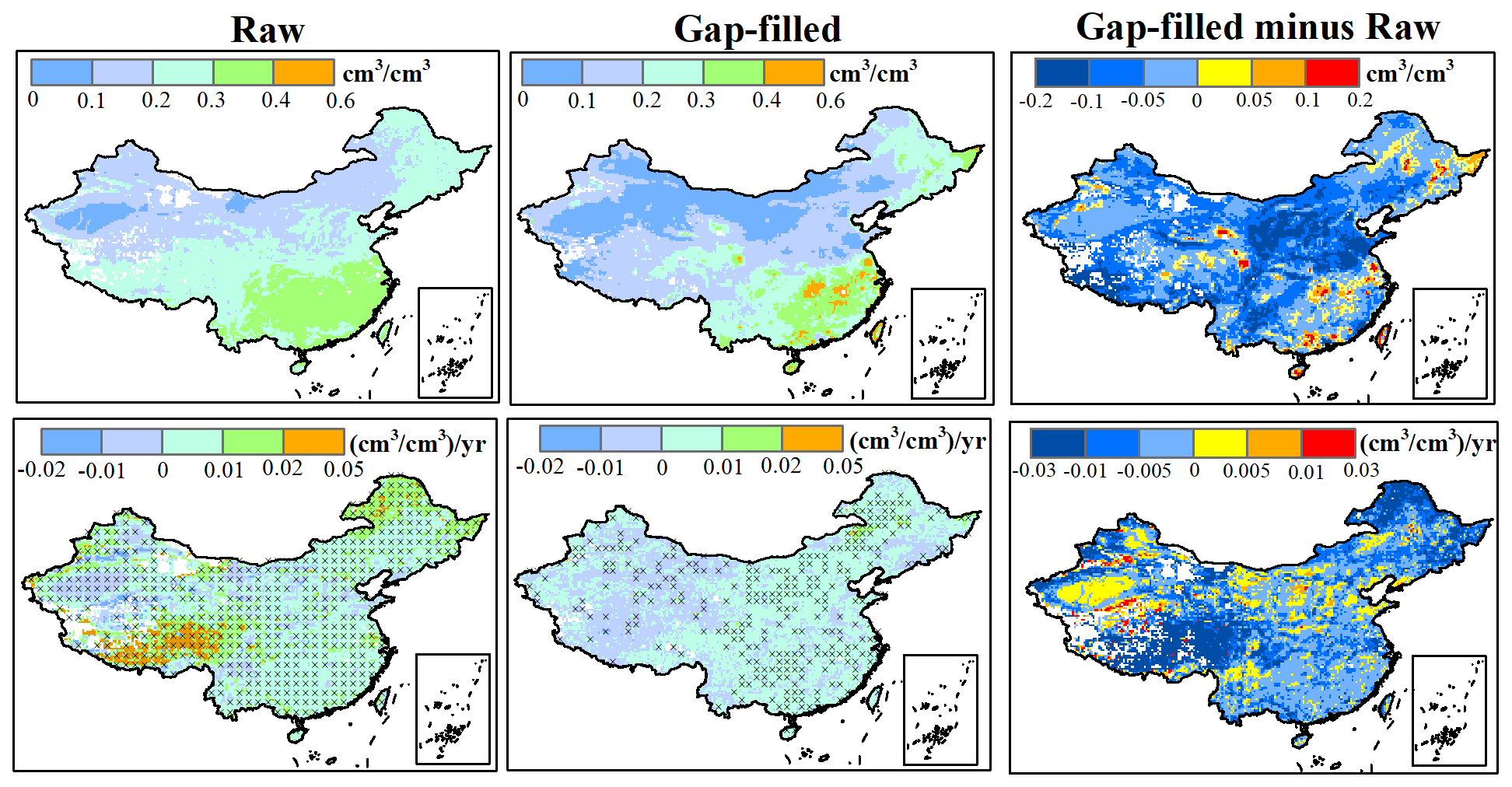
Figure 13 Implementation of the proposed model in 2005–2015. Panels (a) and (b) are the average values of raw CCI and gap-filled SM during 2005–2015, and panel (c) is the difference between them. Panels (d) and (e) are the average trends of raw CCI and gap-filled SM during 2005–2015, and panel (f) is the difference between them. The “x” symbol in panels (d) and (e) denotes the significance level under 0.05.

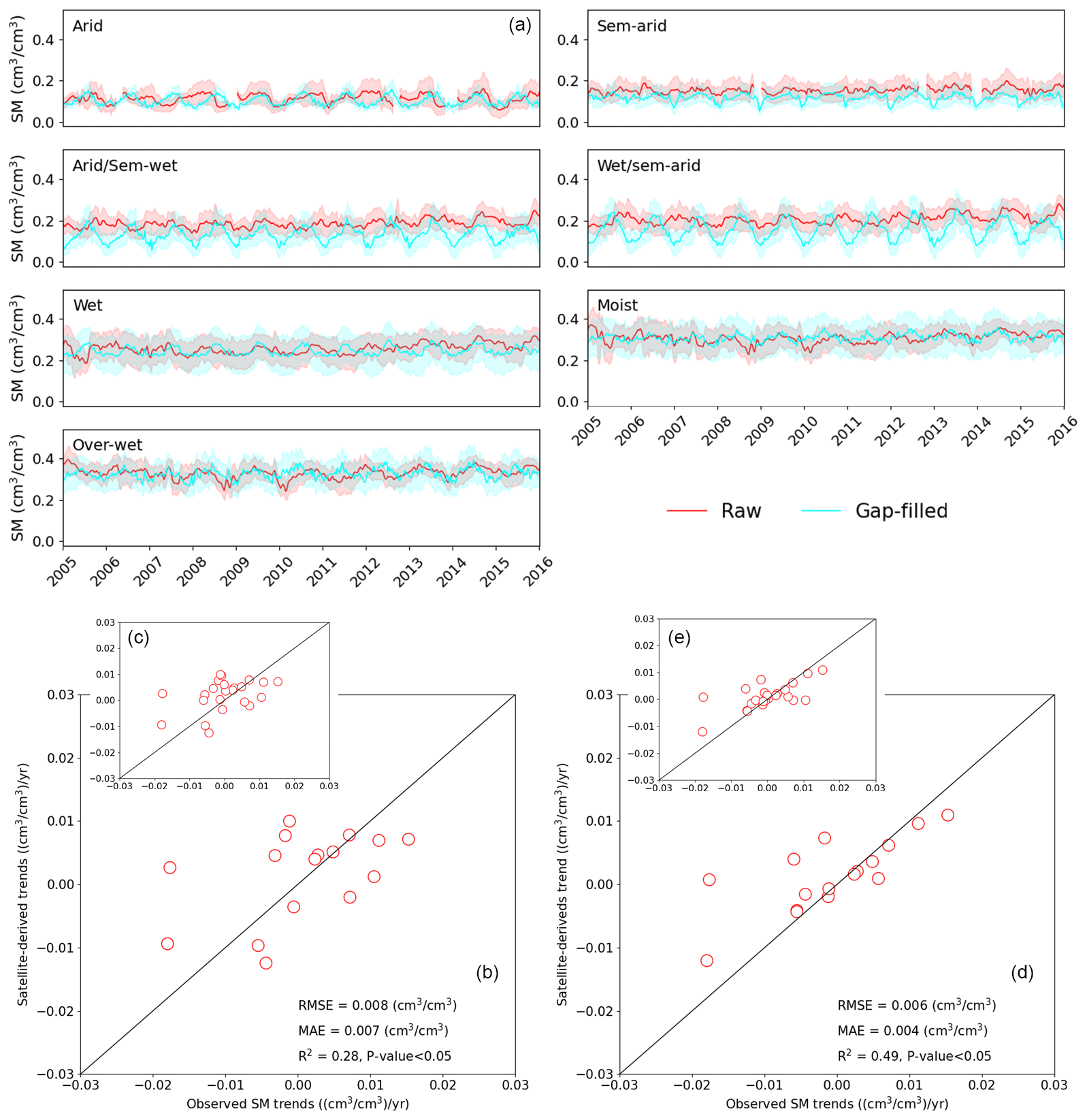
Figure 14 Panel (a) shows the temporal patterns of raw and gap-filled CCI SM regarding different climate regions during 2005–2015. The shaded area in panel (a) denotes ±1 standard error. (b) and (c): scatter plot of 1 km CCI SM-derived trends against in situ measures during 2005–2014, and panel (b) shows the trends under the significance level, while panel (c) shows all the trends. (d) and (e): scatter plot of 1 km gap-filled SM-derived trends against in situ measures during 2005–2014, and panel (d) shows the trends under the significance level, while panel (e) shows all the trends.

Table 2 Metrics for the gap-filling performance regarding the Maqu network for the extended years.

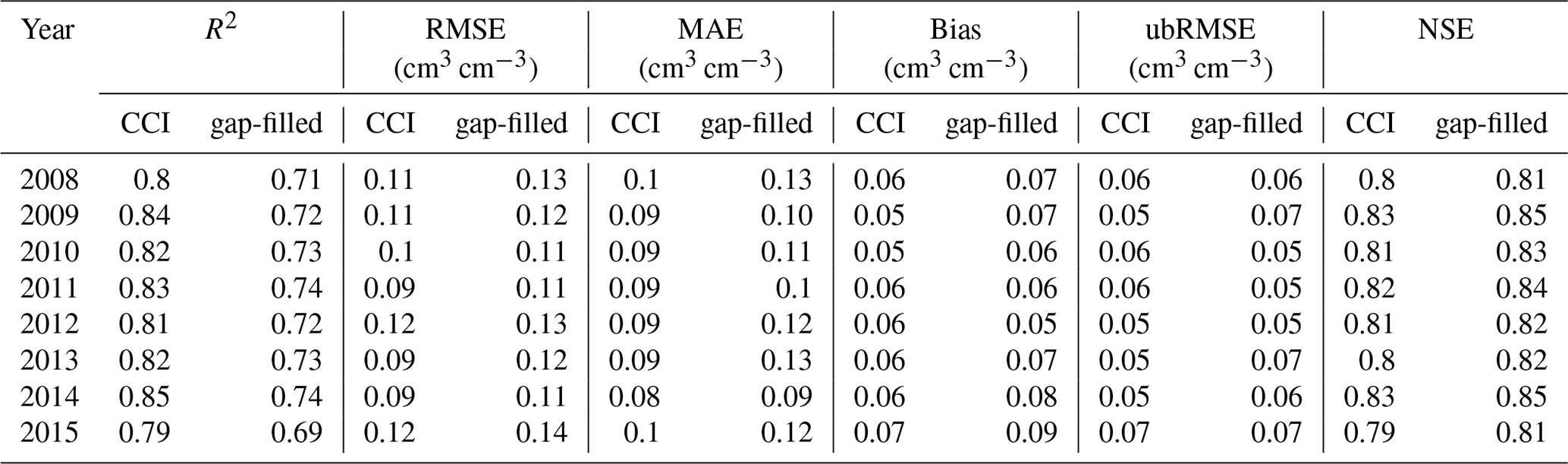
Note: NSE is from the evaluation with the time series of average 0.25^∘ pixels, while the other five metrics are from the evaluation with 1 km disaggregated values.

We further investigate the substitution performance of other surface temperature products in reconstructing SM. Considering the bias between satellite-derived LST and modeled surface temperature, the variable correction described in Sect. 3.1.5 is conducted to remove the systematic bias and make the simulated DTR comparable with the satellite observations. Minor reductions are found in the Pearson correlation and RF-derived importance score of three numerical model-simulated DTRs (Fig. S6) when compared with the MODIS-derived DTR, which indicates the feasibility of using each of these datasets in reconstructing SM. Reductions in model accuracy are evident when replacing the satellite-derived LST with the other three simulated sources (Fig. 12a and b). Nevertheless, the availability of reconstructed SM products is remarkably increased (by ∼ 6 %–11 %) owing to the all-weather coverage of the reanalysis and land surface model simulations. The surface temperature source from the numerical model dataset is suggested as an alternative for satellite LST, which is essential on the long-term and large extended scale, especially considering their full-coverage characteristic. However, in comparison with the results obtained using the correction procedure, reduction in accuracy metrics (∼4 %) occurs when not considering the variable correction procedure. It emphasizes the indispensable contribution of the variable calibration procedures in reconstructing surface characteristics (Duan and Bastiaanssen, 2013; Liu et al., 2020a).

We also compare the ERA SM with two other products to evaluate its feasibility in reconstructing CCI SM. GLEAM and Noah surface SM are separately employed to replace the ERA SM while keeping other explanatory variables the same. Although the GLEAM and Noah SM-based schemes can demonstrate acceptable accuracies, they exhibit slightly inferior accuracies in comparison with the ERA SM-based schemes, probably owing to their relatively large uncertainties in depicting the surface SM dynamics across the two selected regions. Nevertheless, our study focuses on only two local regions; therefore, we cannot claim that the ERA product could provide the best performance across China, and more attention should be focused on this in further work.

4.6 Long-term extension

The proposed gap-filling method is further extended to the long-term ECA CCI SM databases. During 2005–2015, more than 90 % of contaminated pixels can be reconstructed using our model. When evaluating the pixels against in situ measurements from the dense Maqu network, we observe that the reconstructed SM during 2005—2015 has an accuracy that is comparable to that in 2009 (Table 2). The average R² and RMSE values of the reconstructed SM are 0.73 and 0.12 cm³ cm⁻³, respectively. The present results indicate that the proposed model has a strong capacity to simulate SM on the long-term scale.

The spatial distribution and the obvious differences between the gap-filled and original SM datasets can be seen in Fig. 13a–c. The gap-filled SM is drier overall than the raw SM, consistent with the findings from Fig. 5. Negative differences in SM occur in most regions, while positive differences are evident in small areas of the wet and arid regions. The dynamics and trends of SM are fundamental to assessing and quantifying ecohydrological regimes. As shown in Fig. 13d–f, the difference in valid participating SM values causes disparity in calculating the SM trend, i.e., bringing a lower SM trend in most wet regions but a higher SM trend in some dry regions when gap-filled values are introduced. It implies that the trends in SM could be overestimated in satellite products because they were missing. Additionally, most regions with a significant trend demonstrate a lower trend in comparison with the trends of the original SM. The confidence level of the SM trend is converted from a significance level to a non-significance level for a considerable fraction of the grids. This is more pronounced in wet regions such as the northeastern, northwestern, and southwestern parts of China, which are sensitive to monsoon precipitation and ice melting.

The biases in SM dynamics and trends are shown more pronounced for each climate region in Fig. 14a and b. The regional averages of reconstructed SM are relatively low in comparison with those from the original CCI SM. The improvement in the reconstructed dataset in depicting SM trends is quantitatively manifested in Fig. 14c–f; that is, the R² value between the trends from the original CCI SM and those from the in situ measurements is 0.28, while the R² value between the trends from the reconstructed CCI SM and those from the observations is increased to 0.49. Our results are corroborated by earlier studies (Zhang et al., 2018; Gunnarsson et al., 2021) that revealed an overestimation in the trend of missing aerosol optical depth and albedo when cloudy conditions prevented satellite retrievals. It means that the variations in SM trend are related to changes in the climate variables (e.g., precipitation) and land management activities (Li et al., 2018).

5 Conclusions and future considerations

The continuity of satellite-derived SM series is hampered by data gap problems. This study provides a novel framework for reconstructing a spatially continuous daily SM dataset by integrating the European Space Agency CCI SM and related explanatory variables. To achieve this, the random forest method taking full account of both the spatial and temporal domains is adopted. The explanatory variables filtered based on a spatiotemporal window search strategy exhibit a substantial effect in driving the RF regression, resulting in an efficacy improvement of ∼19 %. Meanwhile, model performance is enhanced by calibrating the derived residuals based on geographical weight regression and Gaussian filters. This improvement is manifested by the fact that the accuracies of gap-filling models are lowered by ∼9 % when removing the residual calibration procedure.

Our study illustrates the merit of identifying a sufficient number of explanatory variables from the integration of satellite observations and model-driven knowledge. This is clearly verified by the fact that the accuracy of reconstructed SM is noticeably reduced when excluding one of each of the participating variables in turn while retaining the remaining variables. The selected variables complementarily reproduce the SM dynamics in addition to capturing the spatial variations, which also implies that the nonlinear correlation between the SM and explanatory variables can be depicted on the spatiotemporal scale. In addition to the conventional variables from optical remote sensing, the essential environmental elements from model-driven knowledge are used to improve the performance of SM reconstruction. Earlier studies have suggested (Li et al., 2021a; Long et al., 2019; Shangguan et al., 2017) that reanalysis datasets and land surface model products could provide spatiotemporally continuous records, indicating the great potential of simulating land surface parameters. Here, we employ a machine learning model and a bias correction procedure for CCI SM simulation, which is expected to leverage the knowledge of the reanalysis dataset and the output from the land surface model in transfer to the CCI SM time series. The reconstructed SM achieves satisfactory accuracy over China, underscoring the importance of spatial coverage and continuity of the environmental factors from model-driven knowledge and highlighting the need for multiple datasets to be involved in gap-filled models. We further confirm this with an uncertainty analysis showing the feasibility of using alternative data sources of DTR and SM, which is essential on the long-term scales, considering the full coverage characteristic of numerical-model-simulated products. Nevertheless, because numerical simulation models are generally sensitive to regional surface and climatic conditions, adoption of more effective machine learning models and bias correction strategies as well as more representative model outputs such as CLDAS and regional numerical models could be considered in further work (Li et al., 2022a, b).

Machine learning is recognized as a powerful tool for reconstructing contaminated values. Despite the effectiveness of the RF model for in situ SM databases, its applicability to reconstructing long-term satellite observational records, especially on the large scale, deserves careful investigation. Here, we further confirm that the RF, combined with appropriate covariates exploiting both the spatial and temporal domains together with a model-derived residual calibration module, could be a robust method for gap filling of the CCI SM database over China. The superiority of the RF-based model in reconstructing SM is further proved by comparison with four other models. Nevertheless, more advanced machine learning strategies, such as deep neural networks (DNNs) and long short-term memory (LSTM), are expected to enhance simulation accuracy. Ensemble approaches that mainly account for the scale biases among different gridded datasets are required. For example, development of a Bayesian modeling framework that can provide simulation standard error using uncertainty quantification is encouraged (Zhao et al., 2019a).

The variables forcing the proposed model are all available on the long-term scale globally. Accordingly, our framework could be extended to generate a promising long-term gap-filled SM dataset. This is critical considering that spatiotemporally continuous SM is required for ecological and hydrological research. Thus, the findings of our study might provide insights regarding continuous monitoring of surface water dynamics and drought and promote further research into water resource management and climate change.