Assessment of plot-scale sediment transport on young moraines in the Swiss Alps using a fluorescent sand tracer

Glacial retreat uncovers large bodies of unconsolidated sediment that are prone to erosion. However, our knowledge of overland flow (OF) generation and sediment transport on moraines that have recently become ice-free is still limited. To investigate how the surface characteristics of young moraines affect OF and sediment transport, we installed five bounded runoff plots on two moraines of different ages in a proglacial area of the Swiss Alps. On each plot we conducted three sprinkling experiments to determine OF characteristics (i.e., total OF and peak OF flow rate) and measured sediment transport (turbidity, sediment concentrations, and total sediment yield). To determine and visualize where sediment transport takes place, we used a fluorescent sand tracer with an afterglow as well as ultraviolet (UV) and light-emitting diode (LED) lamps and a high-resolution camera. The results highlight the ability of this field setup to detect sand movement, even for individual fluorescent sand particles (300–500 µm grain size), and to distinguish between the two main mechanisms of sediment transport: OF-driven erosion and splash erosion. The higher rock cover on the younger moraine resulted in longer sediment transport distances and a higher sediment yield. In contrast, the higher vegetation cover on the older moraine promoted infiltration and reduced the length of the sediment transport pathways. Thus, this study demonstrates the potential of the use of fluorescent sand with an afterglow to determine sediment transport pathways as well as the fact that these observations can help to improve our understanding of OF and sediment transport processes on complex natural hillslopes.

1 Introduction

Soil erosion rates in alpine regions are high (Panagos et al., 2015; Gianinetto et al., 2020; Musso et al., 2020a) and are expected to increase because of climate change. Rapid glacier retreat exposes unvegetated areas that are prone to surface erosion (Klaar et al., 2015). These changes will affect water quality (Brighenti et al., 2019; Colombo et al., 2019), fish habitats (Carnahan et al., 2019; Cowie et al., 2014), and the longevity of hydropower reservoirs (Li et al., 2022). Climate change is expected to also increase the frequency, intensity, and amount of heavy precipitation (Gobiet and Kotlarski, 2020; Gobiet et al., 2014), which also affects erosion rates and sediment yield (Anache et al., 2018; Maruffi et al., 2022; Nearing et al., 2004). Splash erosion (i.e., the detachment of soil particles by the impact of raindrops) is positively correlated with rainfall intensity (Angulo-Martínez et al., 2012; Fernández-Raga et al., 2017; Park et al., 1983) because the larger raindrops during intense rainfall have a higher kinetic energy (Evans, 1980). If the rainfall intensity is higher than the infiltration capacity of the soil, infiltration-excess overland flow (i.e., Hortonian overland flow, HOF; Horton, 1933) occurs. Saturation-excess overland flow (SOF) occurs during (long) rainfall events that saturate the soil. HOF and SOF can transport the detached particles downslope via interrill erosion or where flow is concentrated via rill erosion.

Whether overland flow (OF) can transport the detached particles to the bottom of a hillslope or to the stream depends on the connectivity of the source areas to the slope bottom or stream, i.e., whether the two points are connected by water flow (Bracken and Croke, 2007; Smith et al., 2010). This depends on the degree to which transport is facilitated or impeded by surface characteristics and processes. If water infiltrates into the soil after a short distance (i.e., the OF pathways are short), then the OF water and the sediment it carries may not reach the bottom of the hillslope. Thus, sediment connectivity depends on the amount of OF and variability in OF, which is affected by the precipitation amount and intensity, the antecedent soil moisture conditions (Nanda et al., 2019), the spatial variability in infiltration rates (Vigiak et al., 2006; Gerke et al., 2015; Cammeraat, 2002), the microtopography (Appels et al., 2016), and the vegetation type and cover (Dunne et al., 1991; Thompson et al., 2010b; Wainwright et al., 2000).

The importance of surface hydrological connectivity for sediment yield is well established (see, e.g., Bracken et al., 2015; Heckmann et al., 2018; Najafi et al., 2021). Several studies have defined hydrological connectivity (Bracken et al., 2013; Bracken and Croke, 2007) or sediment connectivity indices (Heckmann and Schwanghart, 2013) to quantify the degree to which a system facilitates the transfer of water and sediment (e.g., Asadi et al., 2019; Gay et al., 2016; Heckmann et al., 2018; Lane et al., 2009; Shore et al., 2013; Zanandrea et al., 2021). Connectivity has also been implemented in different conceptual frameworks (Brardinoni and Hassan, 2006; Stock and Dietrich, 2003; Bracken et al., 2013; Bracken and Croke, 2007; Reaney et al., 2014) and explored in various model studies (Appels et al., 2011; Reaney et al., 2014; Masselink et al., 2017; Peñuela et al., 2016). Much less is known about the real-world connection of OF pathways (Wolstenholme et al., 2020) and how this affects sediment transport because it is difficult to observe OF pathways and sediment transport during rainfall events. This is particularly the case for vegetated hillslopes, but some studies have managed to do so by mapping sediment and flow pathways after events (Marchamalo et al., 2016) or by mapping erosion and deposition areas (Calsamiglia et al., 2020).

Connectivity of OF has been studied in arid areas (Smith et al., 2010; Moreno-De Las Heras et al., 2010; Lázaro et al., 2015), agricultural areas (Peñuela et al., 2016; Sen et al., 2010; Buda et al., 2009), and on frozen soils (Coles and McDonnell, 2018). Dyes and cameras (Polyakov et al., 2021; Wolstenholme et al., 2020; Smith et al., 2010; Gerke et al., 2015) and thermal imaging of heated water (Lima et al., 2015) have been used in rainfall simulation studies on laboratory flumes and in arid areas. For example, Wolstenholme et al. (2020) used visual observations of the OF pathways and highlighted the importance of infiltration along the flow path and flow resistance for the establishment of connectivity. They also stressed the importance of vegetation, slope, surface stone cover, and surface roughness for OF generation in dryland areas. Marchamalo et al. (2016) used repeated field mapping in semiarid catchments to determine the connectivity between sediment source areas and sediment sinks. Calsamiglia et al. (2020) used uncrewed aerial vehicles (UAVs) and field mapping to, similarly, study the evolution of surface flow pathways and the erosion and deposition of sediment after storm events in a small agricultural catchment. Other studies used radio frequency identification tags (Parsons et al., 2014), diffuse reflectance spectrometry (Martínez-Carreras et al., 2010), and rare earth element tracers (Polyakov and Nearing, 2004; Deasy and Quinton, 2010) to study sediment transport and connectivity. For example, Guzmán et al. (2015, 2010) used silt-sized magnetite, hematite, magnetic iron oxide, and goethite particle tracers mixed into soil aggregates to study sediment movement on agricultural fields. The tracer and sediment concentrations were measured in the runoff at the bottom of the plots, but no observations were made on the plot surface to determine the actual flow pathways. Tauro et al. (2012b) used buoyant fluorescent polyethylene spheres to determine particle transport velocities on seminatural hillslopes. They showed that Full HD videos were best for real-time detection of the movement of these rather large spheres (1.0–1.2 mm). However, their fluorescent spheres did not have the same shape as natural soil particles and also had a different buoyancy (i.e., the particles could float on the water). Sand particles coated with a fluorescent paint represent the size and density of natural soil particles more closely than fluorescent spheres and have been used to track sediment movement on beaches (Ingle, 1966), along the surf zone in the Nile Delta (Badr and Lotfy, 1999), to study on- and offshore sediment transport along the coast of Israel (Klein et al., 2007), and to examine sand movement in a river tidal flat in Japan (Kato et al., 2014). Hardy et al. (2017, 2019) used a fluorescent sand tracer with a similar particle size and density to the soil in order to study soil redistribution by tillage on arable farmland. Although pioneering studies using fluorescent sand (Yasso, 1966) and glass particles (Young and Holt, 1968) considered it suitable for sediment transport studies more than 5 decades ago, they have so far not been used to determine the rates of sediment movement on natural hillslopes (Parsons, 2019).

Therefore, we tested the use of a fluorescent sand tracer in combination with sprinkling experiments to study sediment transport on two young moraines in the Swiss Alps. The moraines differed in age (one had only been ice-free for 3 decades, whereas the other had been ice-free for more than 1.5 centuries) and, therefore, surface characteristics (e.g., vegetation cover, rock cover, surface roughness, aggregate stability, and saturated hydraulic conductivity). More specifically, we assessed the following research questions:

• Can fluorescent sand particles be used to trace sediment transport on young moraines?

• Do the derived differences in sediment transport distances explain the differences in sediment concentrations and sediment yield at the bottom of the plot?

• How are sediment yield and sediment transport distances related to the surface characteristics (slope, vegetation cover, surface roughness, soil aggregate stability, and saturated hydraulic conductivity)?

We hypothesized that higher rainfall intensities lead to more OF and sediment transport (Medeiros and de Araújo, 2013; Buendia et al., 2016; van De Giesen et al., 2000) and that there would be more OF on the older moraine due to the lower infiltration rates into the finer matrix (Lohse and Dietrich, 2005; Maier et al., 2020). However, we expected that sediment transport distances would be shorter and erosion rates would be lower for the older moraine due to the higher vegetation cover (Geißler et al., 2012; Greinwald et al., 2021a). Furthermore, we expected that the higher surface roughness and larger depression storage for the younger moraine, as well as the higher effective infiltration rates in these depressions, would lead to a decrease in connectivity and sediment yield (see Govers et al., 2000).

2 Site description

2.1 Study area

The field measurements were conducted between August and September 2018 in the forefield of the Steigletscher (also known as Stein Glacier), south of the Susten Pass mountain road in the central Swiss Alps (46^∘43^′ N, 8^∘25^′ E; Fig. 1). The elevation of the glacial forefield ranges between 2000 and 2100 m a.s.l. (meters above sea level). The study area is part of the internal alpine massif (Aarmassif) and underlain by the highly polymetamorphic Erstfeld Gneiss Complex. It predominantly contains biotite–plagioclase–gneiss, pre-Mesozoic metagranitoids, and amphibolites (Labhart, 1977).

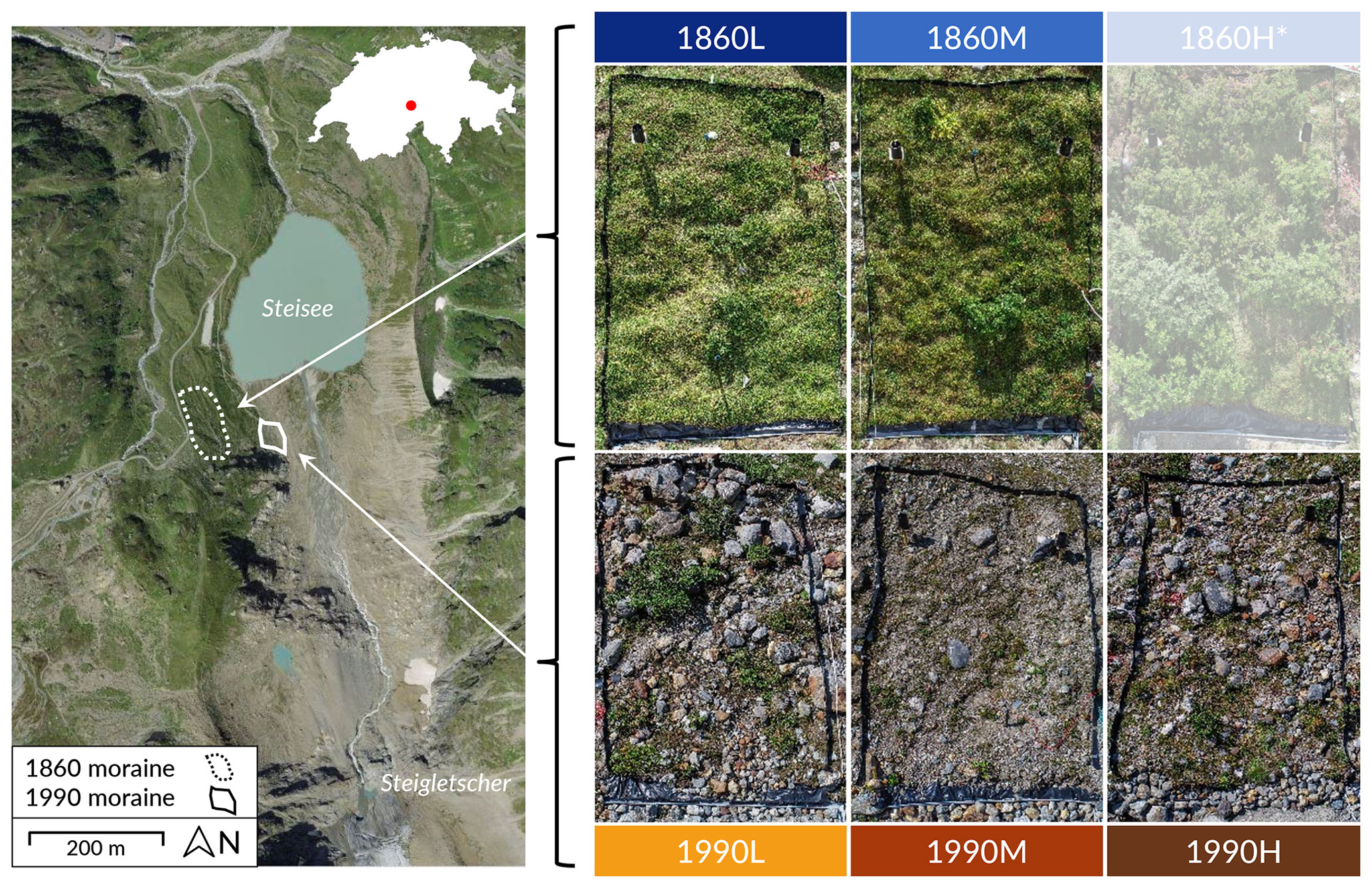
Figure 1 Aerial image of the Susten Pass study area (left panel) and photographs of the three experimental plots (right panel) on the 1860 and 1990 moraines. The outlines of the two studied moraines are indicated on the aerial image of the study area (1860 moraine: dashed line; 1990 moraine: solid line). The vegetation cover for the older (1860) moraine (right panel, top row) is much higher than for the younger (1990) moraine (right panel, bottom row). The 1860H plot was excluded from the analyses due to the dense shrub cover. The aerial image was sourced from the Federal Office of Topography Swisstopo (“A journey through time”, 2019).

The mean annual air temperature (1991–2020) at the closest long-term automatic weather station (the Grimsel Hospiz, located 20 km from the study area at 1980 m a.s.l.) is 2.3 ^∘C (MeteoSwiss, 2022). The average monthly temperature for the same period varies between −4.9 ^∘C in February and 10.3 ^∘C in August. The mean annual precipitation at the Grimsel Hospiz is 1834 mm yr⁻¹, and it is evenly distributed over the year. Snowfall events are frequent, even during the summer months. On average, there is more than 10 cm of snow on the ground for 210 d yr⁻¹ (MeteoSwiss, 2022). Even though streamflow is dominated by snow and glacier melt, high-intensity rainfall events are also important. The 30 min rainfall intensity with a 10-year return period is 36 mm h⁻¹ (95 % confidence interval of 30–46 mm h⁻¹, 1990–2020 period; MeteoSwiss, 2021).

Based on glacier extent maps for the last 150 years and aerial images (the Swiss Federal Office of Topography “A journey through time – maps” and the SWISSIMAGE 10 cm “A journey through time – aerial images”), we selected two moraines that could be dated precisely (Fig. 1). The older moraine originates from the Little Ice Age (hereafter called the “1860 moraine”), while the younger moraine only became ice-free in 1990 (hereafter referred to as the “1990 moraine”; see Musso et al., 2020b; Maier and van Meerveld, 2021). Both moraines were located ∼ 900 m north from the terminus of the Steigletscher in 2018. The 1990 moraine is located ∼ 30 m higher than the 1860 moraine. Both moraines are side moraines and are northeast-exposed.

The 1860 moraine is largely covered by alpine sweet vernal grass (Anthoxanthum alpinum), bellflowers (Campanula scheuchzeri), pale clover (Trifolium pallescens), and willow (Salix retusa and Salix glaucoserica; Table 1). The 1990 moraine is dominated by fields of scree (Table 1) and pioneer plant species, such as pale clover (Trifolium pallescens), alpine bluegrass (Poa alpina), and alpine willowherb (Epilobium fleischeri; Table 1). Typical early-successional communities on coarse-textured soils, such as Salix retusa and Salix hastata with shallow root systems (Hudek et al., 2017; Jonasson and Callaghan, 1992; Lichtenegger, 1996; Pohl et al., 2011) can be found on the 1990 moraine as well. Vegetation cover, root density, and organic matter content are higher for the 1860 moraine than the 1990 moraine (Greinwald et al., 2021b).

Table 1 Overview of the main characteristics (elevation, slope, aspect, dominant species, vegetation cover, rock cover, sand content of the upper 10 cm of the soil, and the tortuosity index) for the five study plots.

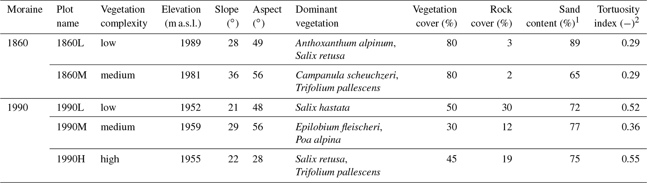
¹ Information sourced from Hartmann et al. (2020b). ² Values calculated using the method of Bertuzzi et al. (1990), based on the normalized line length for 10 measurements on
each plot with a microtopography profiler of 1.5 m length (see Leatherman, 1987).

The soils of both moraines are sandy-loam Hyperskeletic Leptosols, are very young, and contain coarse gravel fragments, sand, and buried stones throughout the profile (Musso et al., 2019). The soil texture in the upper 50 cm of soil is similar for the two moraines, with sand (particle diameter 63 µm–2 mm) being the dominant texture (∼ 75 %; Hartmann et al., 2020a).

2.2 Study plots

On each moraine, we installed three 4 m × 6 m bounded runoff plots (Fig. 1, Table 1). To cover as much variability as possible on each moraine, we chose the location of the plots based on vegetation cover and functional diversity (Garnier et al., 2016; Maier et al., 2020; Greinwald et al., 2021b). More specifically, we selected the area with the lowest (L), intermediate (M), and highest (H) vegetation complexity on each moraine (Table 1; Maier and van Meerveld, 2021). Vegetation complexity is an index based on the vegetation cover, number of different species, and functional diversity (based on stem growth form, root type, clonal growth organ, seed mass, Raunkiær's life-form, leaf dry-matter content, nitrogen content, and specific leaf area; Garnier et al., 2016; Greinwald et al., 2021b). The vegetation cover was 80 %, 80 %, and 95 % for the L, M, and H plots on the 1860 moraine and 50 %, 30 %, and 45 % for the L, M, and H plots on the 1990 moraine, respectively (Fig. 1, Table 1). Because the 1860H plot was covered with dense shrubs of alpine rose that obscured the fluorescent sand, this plot was not included in any of the analysis (i.e., we report the results for five plots only). The plots were all steep, with the average slope varying between 21^∘ and 36^∘ (Table 1). However, the topographic position of the plots differed. The 1860L, 1860M, and 1990M plots were located at a mid-slope position, whereas the 1990L and 1990H plots were located at the bottom of the slope.

3 Methods

3.1 Plot characteristics

3.1.1 Surface topography and rock cover

The slope angle for the plots was determined based on 12 measurements with an inclinometer (every 50 cm on both sides of each plot). We report the average value for the seven measurements on the bottom half of the plots where the fluorescent sand and blue dye were applied (see Table 1). We chose to use the inclinometer slope over the slope derived from the digital surface model (DSM; see Sect. 3.4) because of the somewhat coarse resolution of the DSM and the distortion by the vegetation cover. The correlation between the mean slope derived from the DSM and the inclinometer measurements was high (r= 0.94): the difference was less than 3^∘ for all plots.

A 1.5 m long microtopography profiler, consisting of a wooden frame with 101 adjustable 1 m long metal rods (see Leatherman, 1987), was used on 10 transects within each plot to determine the surface roughness based on the normalized line length and the tortuosity index (see Bertuzzi et al., 1990). We report the average values for the six transects on the bottom half of the plots (see Table 1).

Georeferenced and orthorectified photographs from a drone (DJI Phantom 4 Pro; see Fig. 1) were used for visualization of the plots and to determine the rock cover based on a supervised classification in Adobe Photoshop CS6 (v13.0.1; tool: “color range”) that is frequently used for digital image analysis (e.g., Dorador et al., 2014; Zhang et al., 2014). After the plot area was selected with the “marquee” tool, the color range tool (selection preview set to “black matte”) was used to determine the color range of stones and rocks. An automatic algorithm adds pixels that correspond to the color range of the test areas to the selection. The selected pixels (i.e., rocks) were visually compared to the drone image and additional test areas were added until all rocks were selected. Then, the number of selected pixels (determined from the histogram) was divided by the total number of pixels of the plot area to obtain the percentage of rock cover.

3.1.2 Soil aggregate stability

We determined the soil aggregate stability for six soil samples taken from the upper 10 cm of soil at each plot using a HumaxTube^® (GreenGround AG) with the method of Bast et al. (2015). Using this method, the soil sample is placed on a 20 mm sieve and submerged in water for 5 min. The aggregate stability coefficient (ASC) varies between 0 for complete destruction of the soil sample and 1 for a fully stable soil sample (Bast et al., 2015). We report the median ASC value for each plot (see Greinwald et al., 2021a, for more information).

3.1.3 Saturated hydraulic conductivity

Infiltration rates were measured at three locations next to each plot using a double-ring infiltrometer (inner diameter of 20 cm; ASTM D3385-03 standard test method). The infiltrometers were inserted vertically into the ground for at least 5 cm on all sides. The ponding depth was 15–25 cm. The saturated hydraulic conductivity (K_sat) was determined based on the steady-state infiltration rate (see also Maier et al., 2020; Maier and van Meerveld, 2021). We report the average value of the three measurements per plot. We acknowledge that many more measurements would be needed to obtain a robust average K_sat value (e.g., Harden and Scruggs, 2003; Zimmermann, 2008); however, due to time limitations, more measurements were not possible. Nonetheless, the six (1860 moraine) and nine (1990 moraine) measurements at each moraine already provide some information on the magnitude and variability in K_sat.

3.2 Rainfall and overland flow measurements

3.2.1 Plot setup

On the left, right, and upslope borders of each plot, we inserted plastic sheets approximately 5 cm into the ground to minimize lateral in- and outflow of OF from the plots (Fig. 2a). On the downslope border of each plot, we dug a trench and inserted pond foil ∼ 2–5 cm into the soil (Fig. 2b). The foil was attached to a gutter, which was covered with plastic sheeting to protect it from the rain (Fig. 2a). From the gutter, water flowed through a 5 cm diameter hose into an upwelling Bernoulli tube (Stewart et al., 2015), in which a pressure transducer was located (DCX-22-CTD, KELLER). At each moraine, another pressure transducer measured the local barometric pressure. From these measurements, the OF rate could be determined at a 1 min interval. Because the pond foil was inserted several centimeters (up to 10 cm) below the soil surface, the measurements of OF also contain biomat flow (see Sidle et al., 2007) and very shallow subsurface flow (Fig. 2b). However, we refer to this as OF throughout the remainder of this paper. For a more detailed description of the OF measurements, the reader is referred to Maier and van Meerveld (2021).

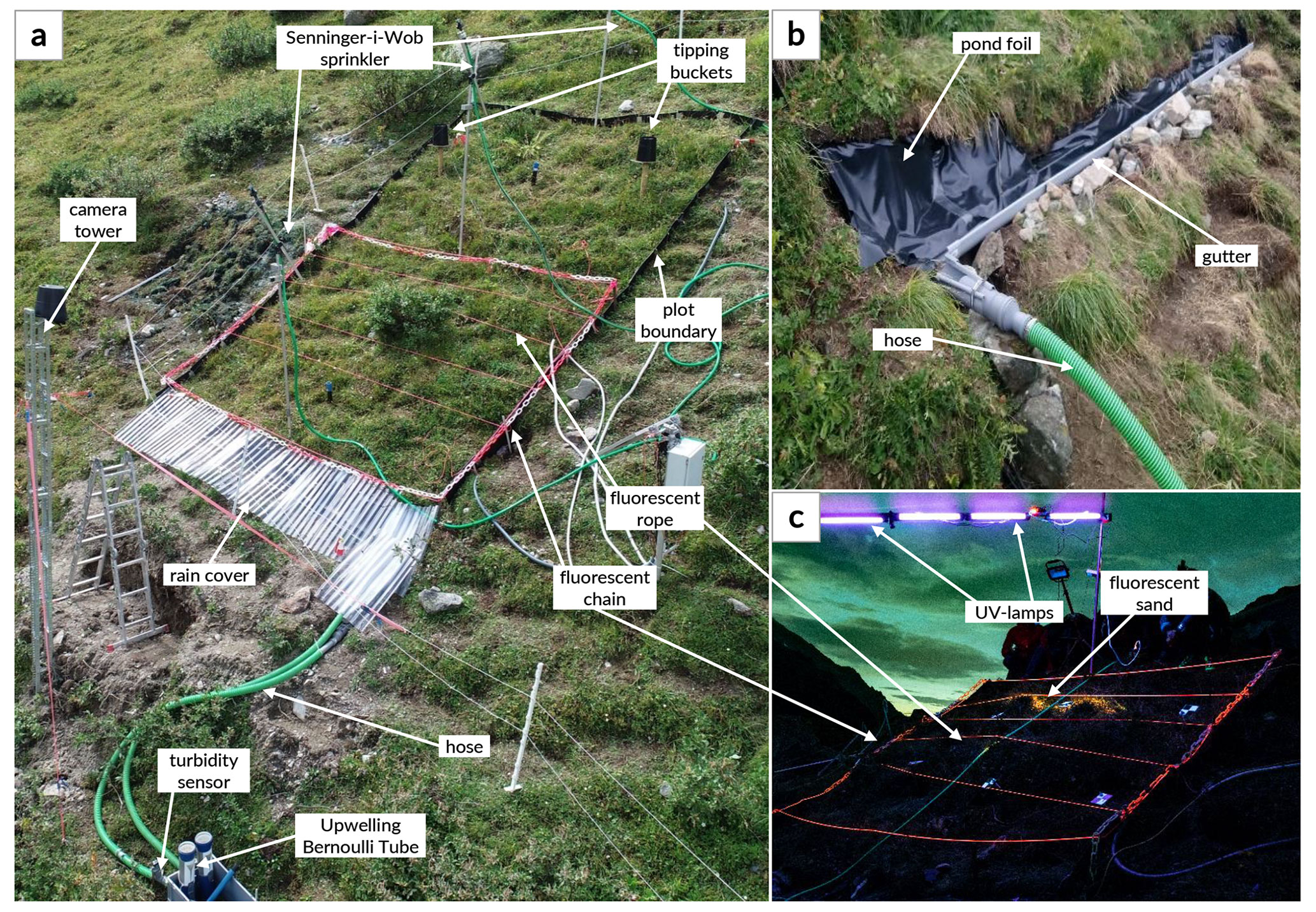
Figure 2 Photos showing the experimental setup for the study plots (a); the collection system for overland flow, biomat, and very shallow subsurface flow (OF) (b); and the setup for the fluorescent sand imaging (c). Important components, such as the plot borders, sprinklers, tipping bucket rain gauges, pond foil, gutter and hose, turbidity sensor, upwelling Bernoulli tubes, fluorescent segmented chain and fluorescent ropes, and camera tower below the plot are marked and labeled. At night, ultraviolet (UV) lamps were used to illuminate the fluorescent sand on the plot (c).

3.2.2 Sprinkling experiments

On each plot, we performed three sprinkling experiments of different intensities over a 3 d time period (Table 2). We refer to these three events as low-intensity (LI), medium-intensity (MI), and high-intensity (HI) experiments. We started the rainfall simulations with the low-intensity (LI) experiment, did the medium-intensity (MI) experiments the next day, and carried out the high-intensity (HI) experiments on the third day. We chose this order to minimize the effect of erosion (and deposition) during the first experiment(s) on sediment transport during the later experiments. If rainfall was expected in the 24 h before the LI experiment or between the experiments, the plots were covered with big tarps. As soil moisture measurements at 5 and 15 cm below the soil surface suggested that the topsoil drains to field capacity within a day and subsurface flow generally stopped within 2 h after rainfall events (Maier et al., 2021), we did the consecutive experiments on each plot 1 d after each other, so that soil moisture was at approximately field capacity for the MI and HI experiments.

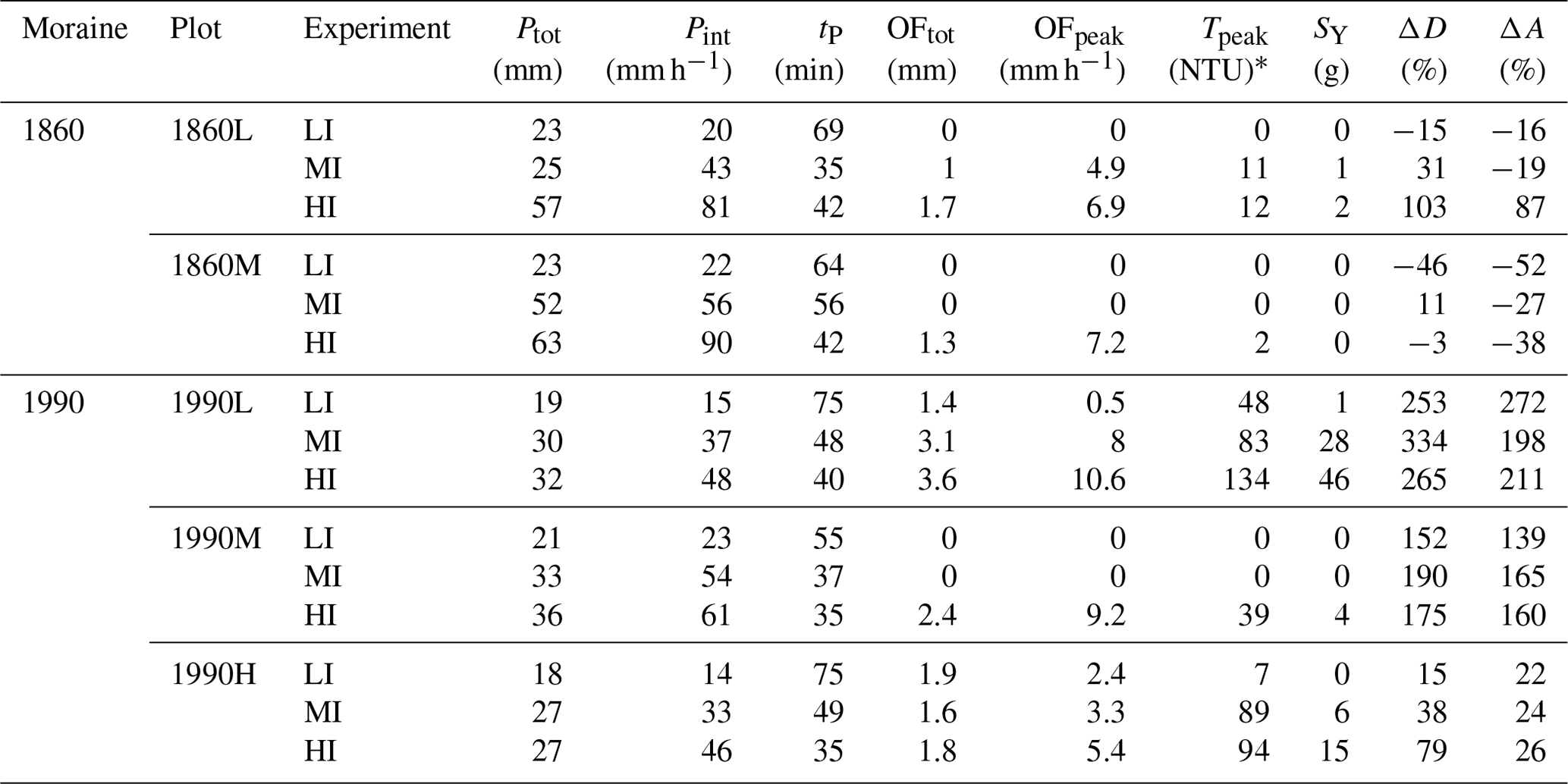
Table 2 Overview of the main response characteristics for all low-, medium-, and high-intensity sprinkling experiments (LI, MI, and HI, respectively) on all five plots. P_tot is the total rainfall amount, P_int is the average rainfall intensity, t_P is the rainfall duration, OF_tot is the total overland flow (OF), OF_peak is the peak OF rate, T_peak is the peak turbidity, S_Y is the sediment yield, ΔD is the percent change in sand distance, and ΔA is the percent change in sand-covered area.

^* NTU denotes nephelometric turbidity units.

We used either one, two, or three Senninger i-Wob adjustable sprinklers (nozzle number 22) to obtain the different rainfall intensities (Fig. 2a). The sprinklers were placed at the center line of the plots at 2 m height (Fig. 2a). The water was obtained from the nearby glacial stream and stored in two 4 m³ water reservoirs, located more than 20 m above the plots to ensure sufficient pressure for the sprinklers. From the reservoirs, water flowed through fire hoses, a water meter, and garden hoses to the sprinklers. The area to which rainfall was applied by the sprinklers extended the plot dimensions by at least 0.5 m upslope and approximately 4 m to the left and right of the plots (as well as several meters downslope). For each experiment, rainfall was applied until total infiltration exceeded 20 mm. The infiltration was determined by subtracting the OF from the applied rainfall. The average sprinkling durations were 68 ± 8 min (LI), 45 ± 9 min (MI), and 39 ± 4 min (HI).

We measured the actual rainfall intensities on the plots using two tipping buckets (Fig. 2a) and at the plot boundaries using four manual rain gauges. The actual rainfall intensities for the LI, MI, and HI experiments varied (Table 2) because of wind drift and differences in the water pressure. The average sprinkling intensities (± standard deviation) were 19 ± 4 mm h⁻¹ (LI), 45 ± 10 mm h⁻¹ (MI), and 65 ± 20 mm h⁻¹ (HI). The mean coefficient of variation in the measured rainfall was 28 ± 15 % (range of 9 %–48 %).

The median drop size at a rainfall intensity of 39 mm h⁻¹, determined using the oil method of Eigel and Moore (1983), was 1.2 ± 0.4 mm (range of 0.4–2.7 mm). This drop size is very similar to the value for natural precipitation in mountain regions in western Europe (∼ 1.1 mm; Hachani et al., 2017) and representative of orographic precipitation (median drop size of 0.1–1.5 mm; Blanchard, 1953). Hence, we assumed that the kinetic energy of our rainfall simulation was comparable to that of natural rainfall in the Swiss Alps.

3.2.3 Suspended sediment measurements

To determine the sediment concentrations in OF, 500 mL samples were taken from the outflow of the upwelling Bernoulli tubes. We started sampling as soon as there was some outflow and continued after the experiment ended until the outflow stopped. More samples were taken on the rising limb than on the falling limb. To determine the amount of sediment per sample, we filtered the samples using 1.6 µm filters (GF/A Whatman) and then dried and weighted the filters. For a more detailed description, the reader is referred to Maier and van Meerveld (2021).

A Cyclops-7 turbidity sensor (Turner designs) was installed between the gutter and the Bernoulli tube (Fig. 2a) and measured the turbidity (in nephelometric turbidity units, NTU) of OF every minute. The turbidity at the time of sampling was related to the sediment concentrations to obtain a moraine-specific relation between the turbidity and suspended sediment concentration. The coefficient of determination (R²) for this relation was 0.80 for the 1860 moraine and 0.89 for the 1990 moraine. The regression slope was 3.1 mg L⁻¹ NTU⁻¹ for the 1860 moraine and 3.3 mg L⁻¹ NTU⁻¹ for the 1990 moraine. These values are comparable to those reported for alpine streams (Paschmann et al., 2017; Geilhausen et al., 2013; Orwin et al., 2010). We used these correlations to obtain time series of the estimated suspended sediment concentration from the turbidity measurements. Finally, the suspended sediment yield was determined for each event based on the sum of the product of the OF rates and the estimated suspended sediment concentrations (see also Maier and van Meerveld, 2021). On the 1990 moraine, some sediment was trapped in the Bernoulli tubes and not sampled. Thus, the sediment yield is slightly higher than estimated this way (estimated error of 1 %–5 % of the total sediment flux per experiment).

3.3 Fluorescent sand transport

To determine where sediment transport occurs and how far individual soil particles are transported along a hillslope during a single rainfall event, we applied ribbons of fluorescent sand to the plots and photographed the plots before and after the sprinkling events. The advantage of the use of fluorescent sand over fluorescent spheres is that the particles have the same size, shape, and density as the material on the moraines and that the sand is a lot cheaper.

3.3.1 Field setup

The night before each sprinkling experiment (10–18 h prior to the experiments), a line of fluorescent sand (glow-in-the-dark sand, Noxton^™) was applied to the soil surface in the middle or lower half of the plot (Fig. 2c). We chose to apply the sand to the lower half of the plots because OF is more likely to occur there due to the larger contributing area than further upslope. The fluorescent sand was placed in ribbons across the surface of the plot using a plastic tube that was cut in half. The tube was filled with the fluorescent sand, placed carefully on the plot, and then slowly turned to release the sand. Thus, the sand covered not only the soil and rocks but also small patches of short vegetation (see Figs. 2 and 8). The applied sand ribbons were about 3–5 cm wide and 2 cm thick. They were 1.5 m long on the 1860 moraine and 3.1 m long on the 1990 moraine. The quartz sand is coated with a nontoxic, photoluminescent (fluorescent and phosphorescent), non-dissolvable powder (TAT33), containing CaAl₂O₄ and Al₂O₃ (Noxton Technologies, 2022). After illumination, the sand has an afterglow for several minutes. The particle size of 300–500 µm corresponds well to the grain size on the moraines, with a median sand (63 µm–2 mm) content of 82 % and 76 % for the top 10 cm of the soil on the 1860 and 1990 moraines, respectively (Hartmann et al., 2020b; Musso et al., 2019). Because the particles have the same density as sand, they are not very susceptible to wind erosion. We used three different colors of fluorescent sand (orange for the LI experiments, green for the MI experiments, and blue for the HI experiments).

3.3.2 Photographs

Pictures of the fluorescent sand were taken the night before and after each sprinkling experiment. A red–white 0.5 m segmented fluorescent plastic chain (Novap) was installed around the bottom half of the plot and served as a reference marker during the image analysis later. In addition, thin red fluorescent ropes were placed every 0.5 m across the plot (Fig. 2a, c) and served as approximate distance markers. In the nights before and after the sprinkling experiments, the fluorescent chain, ropes, and sand were illuminated with six 18W ultraviolet (UV) lamps (Eurolight) for ∼ 10 min before and while taking photographs. These lamps emit light in the UV range at around 365 nm. Four lamps were mounted on a pole that was installed over the plot (Fig. 2c), whereas two were handheld and moved around the plot to illuminate areas in the shadows of rocks or plants. In the ∼ 10 min before the photographs were taken, the sand was additionally illuminated with two 23W light-emitting diode (LED) lights to activate the sand's afterglow. The LED lights were moved to different positions around the plots to illuminate the areas in shadows as well.

A camera (Sony Alpha 7R II) with a wide-angle lens (Sony Vario-Tessar^® T^* FE 16–35 mm F4 ZA OSS) was mounted on a tilting angle (to account for the average slope of the plots) on a 4 m high tower below each plot (Fig. 2a). This camera was used to take photos of the sand ribbons during UV illumination (after LED illumination). The 42-megapixel resolution of the photos (7952 × 5304 pixels) was very good (on the plot surface, 1 pixel corresponds to a length of about 0.5–0.7 mm), which allowed for the detection of individual fluorescent sand particles. The photos were saved with full pixel resolution in RAW format (.ARW file), to obtain a high-quality image with maximum dynamic range, and in JPEG format, for faster post-processing. The aperture was set fully open (F/4). During windy nights, the camera tower moved slightly, which led to blurry photos when slow shutter speeds were chosen. Thus, during windy conditions, the shutter speed was set to 1 s and high ISO values (up to 8000) were used. During nights with little wind, the shutter speed was set to 2, 5, or 10 s to reduce the ISO to 1000–5000 (depending on the light conditions) and obtain better-quality pictures.

On the 1990L plot, we additionally used a liquid brilliant blue dye tracer during the MI and HI experiments to visualize the water flow pathways. We manually added the blue dye tracer to the surface in places where OF was visible. The flow paths of the dye tracer were recorded on video in Ultra HD resolution (3840 × 2160 pixels) with 25 frames per second using the camera (Sony Alpha 7R II) on the camera tower. The combination of several video frames led to a composite picture of the flow paths on the surface, which could then be compared to the movement of the fluorescent sand.

3.3.3 Image post-processing

The photos of the sand ribbons were post-processed to obtain a matrix for each photo, where each element corresponds to one pixel with an area of 1 mm² on the plot (see Schneider et al., 2014; Weiler, 2001; Weiler and Flühler, 2004); an element has a value of one if there was fluorescent sand and zero if there was no sand. These matrices are called classified images in the remainder of the text (Fig. 3b). The procedure used to classify the images is similar to the supervised classification algorithm (maximum likelihood) that is used in remote-sensing analyses (e.g., Richards, 2013).

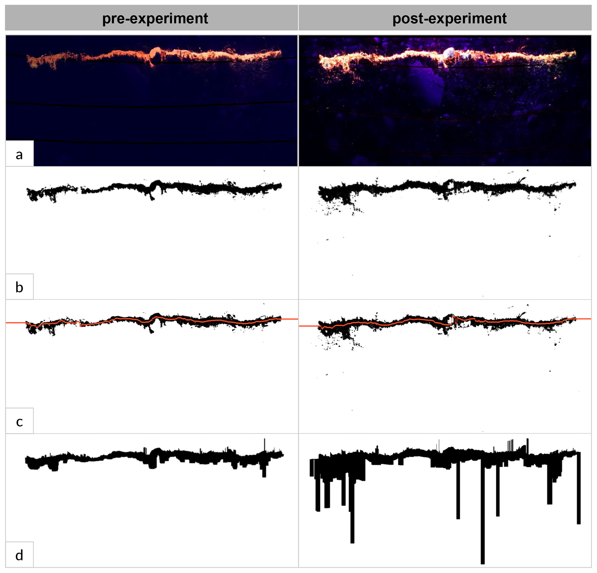
Figure 3 Pre- and post-sprinkling experiment photographs (a) and visualization of the steps taken for the image analysis (b, c, d): geometrically corrected photos with the plot surroundings cut off and the fluorescent ropes digitally removed from the picture (a); classified images (a visual representation of a matrix containing zeros and ones), where classified pixels with fluorescent sand are shown in black (b); classified images with the location of the starting line (in red, at approximately the middle of the sand ribbon) for the determination of sand distances (c); and the calculated areas over which the sand was spread (d). The photos and images shown here are for the 1990M plot before and after the low-intensity (LI) experiment. Please note that, due to the downscaling of the photos and images, not all sand particles are visible in the pictures shown in panel (a).

The segmented chain around the plot was used to determine the location of four points of the chain on the photo (top left-hand corner, top right-hand corner, a point on the bottom left, and a point of the bottom right of the photos). The color of the chain changes every 0.5 m, which facilitated the selection of these points. Known coordinates (measured distances between these points in the field) were assigned to these points. For the resampling, the “skimage.transform.resize” function in Python (v3.8.8) was used within the Scientific Python Development Environment (Spyder v4.1.5). This function uses a Gaussian filter (Gaussian smoothing) to obtain a lower-resolution image from a higher-resolution image while avoiding aliasing artifacts. This “geometric correction” was done for all photos. The areas outside the plots were cropped with Adobe Photoshop CC 2021 (v22.2; Fig. 3a).

The detection of the sand particles was done in the hue, saturation, and value (hsv) color space, which has the advantage that a single number (hue) represents the color. If the hue of a pixel was in the specified range for the sand and the value (v) was above 10 %, the pixel was classified as fluorescent sand. We chose at least 10 representative locations of the sand ribbon on each photo to determine the typical hue of the sand in Adobe Photoshop (orange, 0–80^∘ and 320–360^∘; green, 150–180^∘; and blue, 180–240^∘). As the sand had a certain brightness (due to its afterglow), a value (v) of at least 10 % was chosen to reduce misclassifications in the dark parts (e.g., due to reflections on rocks and vegetation). The classification was done in Python, based on an existing script to detect a brilliant blue dye tracer in soil profiles (Weiler, 2001). To detect the orange sand, the segmented chain and the fluorescent ropes had to be manually removed in Adobe Photoshop because their hue was in the range of the sand. To detect the blue sand, the green sand had to be manually removed in Adobe Photoshop because some green sand particles had a hue within the typical blue sand range (green, 150–190^∘; blue, 180–240^∘).

3.3.4 Image analysis

The fluorescent segmented chain around the plot led to tie areas instead of tie points. Furthermore, they became slightly bent during the experiments (due to their weight). As a result, the reference points for the geometric correction differ for the pre- and post-experiment classified images, i.e., the matrix coordinates (0, 0) in the images classified pre- and post-experiment do not have the exact same position on the plot. This means that the pre- and post-classified images cannot be overlain and subtracted from each other to obtain the change in fluorescent-sand-covered area. Therefore, a theoretical starting line at approximately the middle of the sand ribbon was defined for all classified images (pre- and post-experiment; see Fig. 3c). This assumes that the main part of the sand ribbon did not move during an experiment and only individual sand particles and clusters moved (i.e., the position of this starting line across the middle of the sand ribbon did not change during an experiment). Observations in the field and inspection of the photos confirmed this (e.g., in Fig. 3, the shape of the sand ribbon and its position relative to the rocks remained the same). Based on these starting lines from the classified images, relative measures describing how far the sand moved can be calculated.

More specifically, the starting line in each classified image (pre- and post-experiment) was defined as follows. For every point across the slope (i.e., each individual pixel column i in the classified image), we determined a window of 101 pixels wide (50-pixel columns on each side, representing a 10.1 cm wide section on the plot) and counted the number of pixels that were classified as sand for each row (i.e., every 1 mm upslope from the gutter) within this window. The row with the highest number of classified pixels was considered the starting line for column i and, thus, the starting point for sand movement. If there were several maxima, the median row height was taken as the starting point. If there were only a few (< 30) classified pixels, the value from the neighboring column was used to avoid breaks in the starting line (i.e., there were no gaps in the starting line, even if the sand ribbon itself had a small gap). On the left and right borders of the plot, the moving window was shorter to account for the lack of neighboring points on one side.

We used two measures to describe the movement of the sand during the sprinkling experiments: one related to the distance that the sand moved on the plot (ΔD) and the other to the area over which the sand (ΔA) moved. These two are clearly related to each other but can differ depending on the way that the sand moved across the plot. For each point across the plot (i.e., each column i in the classified images), we determined the distance (x_i) between the starting line and the lowermost pixel that was classified as sand (Fig. 4). We did this for the classified images taken before and after the experiments. The average value of this distance for the classified image taken before the sprinkling experiments represents approximately half of the width of the sand ribbon. Any change in this average distance for the classified image taken after the experiment is an indication of sand movement. This requires that the entire sand ribbon did not move downwards on the plots (which we did not observe; see Fig. 3). Because the sand did not move at most points across the slope, we put extra weight on the particles that were located far from the starting line by using the square root of the mean-squared maximum distance for each column:

$$\begin{array}{}\text{(1)}& D=\sqrt{{\displaystyle \frac{\mathrm{1}}{n}}\cdot {\sum }_{i=\mathrm{1}}^n{x}_i^{\mathrm{2}}},\end{array}$$

where i represents the location across the slope (i.e., the column number in the classified image) and n is the total number of pixels across the plot (i.e., the total number of columns). To calculate how the root-mean-square distance D changed from pre- to post-experiment images, and thus to obtain a measure of the distance that the sand moved during an experiment, the percent change in D (ΔD) was calculated:

$$\begin{array}{}\text{(2)}& \mathrm{\Delta }D=\left({\displaystyle \frac{D_{\mathrm{post}}}{D_{\mathrm{pre}}}}-\mathrm{1}\right)\cdot \mathrm{100}\mathit{\%},\end{array}$$

where D_post is the root of the mean-squared distance of the sand to the ribbon after the sprinkling experiment, D_pre is the root of the mean-squared distance of the sand prior to the sprinkling experiment, and ΔD represents the percent change in the root of the mean-squared distance (increase or decrease in percent) of the sand relative to the middle line of the ribbon. A larger positive value of ΔD indicates that more particles moved further away from the ribbon. A negative value ΔD is also possible and indicates that the sand ribbon became narrower during the experiment. This is possible when sand moved away from the ribbon and was washed into the soil or hidden below vegetation or rocks. True negative distances are also possible due to upslope splash erosion. We did not use the absolute maximum distance or a certain percentile of the maximum distances that the sand moved from the starting line to describe the sand movement because these measures are more sensitive to the detection of individual sand particles than our more integrative measure D. Neither of these approaches account for the transport of the sand off the plots (i.e., into the OF gutters), but D is less sensitive to this than the absolute maximum transport distance.

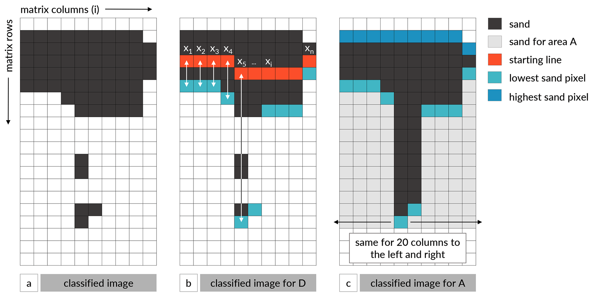
Figure 4 Sketch of the image analysis steps, showing a small part of a classified image where each square represents one pixel or element in the matrix (1 mm² on the plot). Pixels classified as sand are shown in black (a). For the determination of the sand distance (D) in every column i, the distance (x_i) between the starting line (red) and the lowermost sand pixel (shown in turquoise) was determined (b). For the determination of the sand-covered area (A), all pixels between the uppermost (blue) and lowermost sand pixel (turquoise) in each column and the 20 columns to the left and right were considered to be part of area A (c).

As another (but clearly related) measure of the spread of the sand across the plots, we also determined the area with sand (A; Figs. 3d, 4c) and changes therein. We selected all pixels between the furthest downslope and upslope occurrence of sand for each column of the classified images. Sand particles located more than 20 cm above the starting line were not considered, as they were most likely not part of the sand ribbon. To account for the fact that the sand particles probably did not move down the hillslope in a straight line, the uppermost and lowermost (i.e., furthest upslope and downslope) occurrence of sand for each column was calculated for a 41-column window (i.e., 20 columns on each side, representing 2 cm on the plot; Fig. 4). In the case of gaps in the sand ribbon, the interpolated starting line was used to merge all areas into one area (Fig. 4). Similar to the calculation of the sand transport distances, the percent change in the area A (ΔA) was calculated (Eq. 2 but with A instead of D) to determine the change in the area over which the sand was spread during the sprinkling experiments. This ΔA does not represent the actual area over which the sand moved during the experiments (and would overestimate it) but is used here as a measure to compare the spread of the sand during the different experiments on the different plots. A larger positive value of ΔA means that the sand was more spread out across the plot during the experiments. A negative value of ΔA means that the area of sand became smaller, e.g., because the sand moved and was washed into the soil or stored below vegetation and rocks, or moved off the plot (which is not a dominant process because we only observed some fluorescent sand particles in the outflow).

3.4 Digital surface model and flow accumulation

A digital surface model (DSM) derived from drone images of the moraines (drone: senseFly eBee; camera: Sony Cyber-shot DSC-WX220), created using Pix4DMapper by WWL Umweltplanung und Geoinformatik GbR, was used along with the D_∞ routing algorithm of Tarboton (1997) in ArcMap (v10.6.1) to determine the potential direction of OF. The drone-based images had a spatial resolution of ∼ 4 cm, which was considered acceptable for comparison with the results of the movement of the fluorescent sand particles (see Sect. 3.3). However, the DSM (and, thus, also the flow routing) are influenced by vegetation. Because the vegetation was short (< 5 cm, except for two shrubs on the 1860M and 1990L plot) and the plots were steep, this should not have affected the flow directions considerably. Still, we only qualitatively compared these topographically derived flow pathways to the observed patterns of sediment movement and did not use them for any statistical analyses. The other drone (see Sect. 3.1.1) only took pictures of the plots (not the entire moraine) and, hence, could not be used to create a DSM with higher spatial resolution.

3.5 Data analysis

To determine if the differences in the surface characteristics (vegetation cover, rock cover, surface roughness, aggregate stability, and K_sat) for the five plots were statistically significant, we used the Kruskal–Wallis tests and Nemenyi post hoc tests. To determine if the differences in the surface characteristics were significantly different between the two moraines, we used the Mann–Whitney test.

For each event, we determined the total OF, peak flow rate, sediment yield, and peak turbidity. To better compare the OF characteristics between the experiments with different rainfall intensities and amounts, we calculated the OF runoff ratio by dividing the OF amount by the rainfall amount. To determine if the differences in total OF, peak flow, sediment yield, and peak turbidity for the five plots were statistically significant, we used the Kruskal–Wallis tests and Nemenyi post hoc tests. We used Spearman rank correlation (r_s) to determine the correlation between the surface characteristics and total OF, peak flow, sediment yield, and peak turbidity. Similarly, we used Spearman rank correlation to describe the relation between the rainfall intensity and total OF, peak flow, sediment yield, peak turbidity, and the percent changes in sand distance (ΔD) and sand-covered area (ΔA). Due to the differences in slope, aspect, and position of the plots as well as differences in rainfall intensity, we did not expect strong correlations between the individual variables. Therefore, we also used a multiple linear model to predict the change in sand distance and area, using the rainfall intensity as an additional variable. We used the model to identify the interaction between rainfall intensity and the plot characteristics for OF and sediment yield. For the analyses, we used a 0.05 level of significance and the software R (v4.0.5 – used with RStudio v1.4.1106), specifically the following packages: “stats” (R Core Team, 2021), “caret” (Kuhn, 2021), “PMCMRplus” (Pohlert, 2021), “rsq” (Zhang, 2020), and “ggplot2” (Wickham, 2016).

4 Results

4.1 Plot characteristics

4.1.1 Slope and surface roughness

All five plots were relatively steep, with the average slope ranging from 18^∘ on 1990L to 35^∘ on 1860M (Fig. 5a, Table 1). On average, the plots on the 1860 moraine were steeper than the 1990 moraine (29^∘ vs. 26^∘). The differences between the median slopes of the plots (p= 5 × 10⁻⁴) and the two moraines (p= 4 × 10⁻³) were significant. The variability in the slope was largest for the 1990L plot and smallest for the 1990M plot (coefficient of variation, CV, of 0.41 and 0.16, respectively).

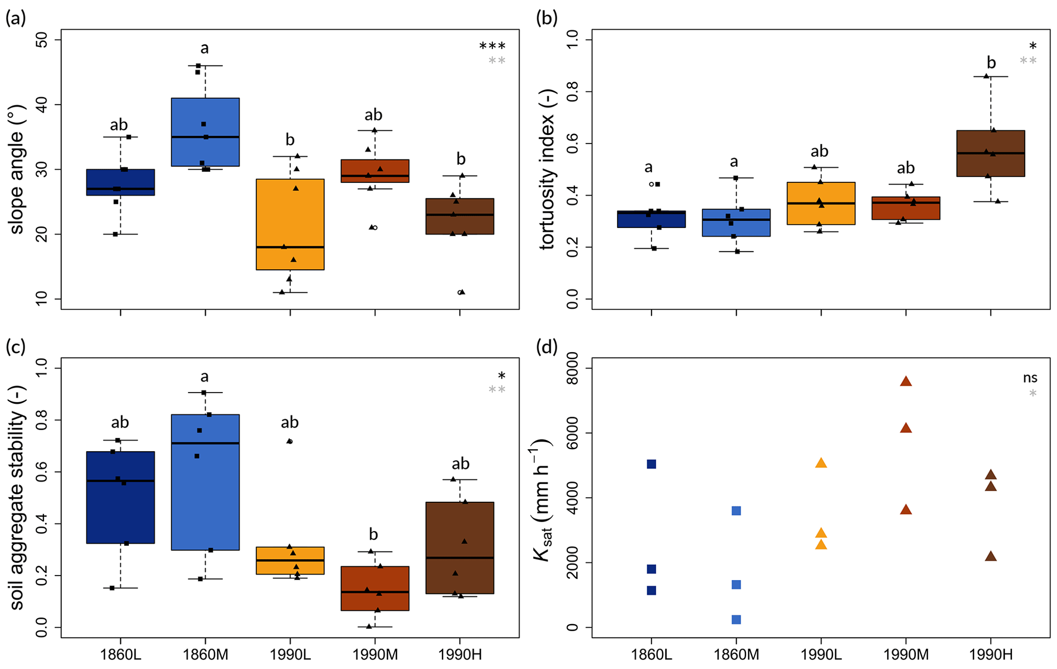
Figure 5 Box plots of the slope angle (a), tortuosity index (b), aggregate stability of the top 10 cm of the soil (c), and saturated hydraulic conductivity (K_sat) of the soil surface (d) for the five different plots. For the box plots, the box represents the 25th to 75th percentiles and the solid thick line denotes the median. The whiskers extend to the 10th and 90th percentiles. The symbols represent the actual measurements (squares for the plots on the 1860 moraine and triangles for the plots on the 1990 moraine). The stars in the upper right-hand corner of the plot indicate the level of significance for the differences in median values for the five plots (top in black font) and between the two moraines (bottom in gray font): ^* for p<0.05, ${}^{**}$ for p<0.01, ${}^{***}$ for p<0.001, and “ns” for p>0.05. Plots that do not share a similar letter (shown above the box plots) are statistically significantly different.

There was also a significant difference in the surface roughness between the plots (p= 0.01; Fig. 5b) and the moraines (p= 7 × 10⁻³). The tortuosity index increased significantly from the 1860 moraine (median of 0.32; range of 0.18–0.47) to the 1990 moraine (median of 0.39; range of 0.26–0.86). The variability in the tortuosity index values was largest for the 1860M plot and smallest for the 1990M plot (CV of 0.32 and 0.15, respectively).

4.1.2 Soil aggregate stability

The aggregate stability of the top 10 cm of the soil (Fig. 5c) differed significant between the plots (p= 0.02; Fig. 5c) and increased significantly from the 1990 moraine to the 1860 moraine (p= 2 × 10⁻³). The median soil aggregate stability coefficient (SAC) was lowest for the 1990M plot (0.14) and highest for the 1860M plot (0.71). The variability in soil aggregate stability was largest for the 1990M plot and smallest for the 1860L plot (CV of 0.74 and 0.44, respectively).

4.1.3 Saturated hydraulic conductivity

The median values of saturated hydraulic conductivity (K_sat) ranged between 1320 mm h⁻¹ (1860M) and 6120 mm h⁻¹ (1990M) and were not significantly different between the five plots (p= 0.12; Fig. 5d). The median K_sat was significantly lower for the 1860 moraine than the 1990 moraine (median values of 1560 and 4320 mm h⁻¹; p= 0.04).

4.2 Overland flow, turbidity, and sediment yield

OF was observed less frequently on the 1860 moraine (three of the six experiments) than on the 1990 moraine (seven of the nine experiments; Fig. 6, Table 2). OF was not observed for any of the low-intensity (LI) experiments on the 1860 plots but was observed for all high-intensity (HI) experiments on these plots. For the 1990 moraine, OF was also observed for all HI experiments; however, for the plots on the footslopes of the moraine (1990L and 1990H), OF was also observed for the LI and medium-intensity (MI) experiments (Table 2). Except for the plots located on the footslopes of the 1990 moraine, the OF runoff ratio (total OF divided by total precipitation) was < 3 %. For the footslope plots (1990L and 1990H), it was 8 %–10 %. The average OF amount (for all experiments on a moraine) was almost 3 times larger for the 1990 moraine (1.8 mm) than for the 1860 moraine (0.7 mm). When looking only at the HI experiments that produced OF on all plots, this difference is smaller (2.6 mm for the 1990 moraine vs. 1.5 mm for the 1860 moraine, or 8 % vs. 3 % of the applied rainfall). The total amount of OF was especially high for the 1990L plot (3.6 mm, or 11 % of the applied rainfall, during the HI experiment; 8.1 mm, or 10 % of applied rainfall, for all three experiments combined; Fig. 6).

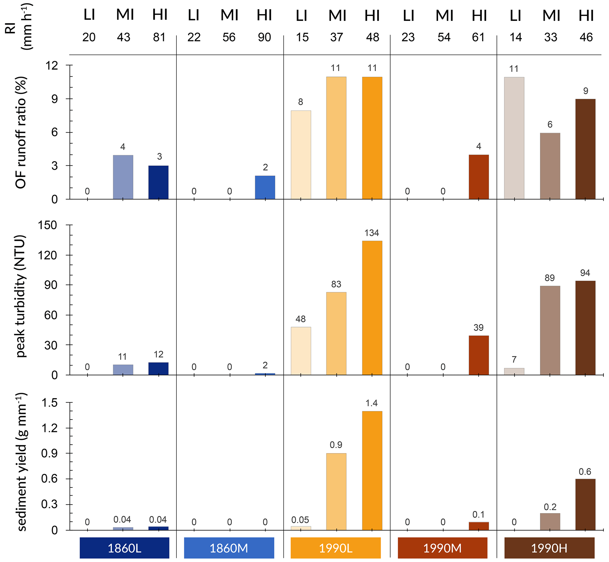
Figure 6 Bar charts of the OF runoff ratio (%), peak turbidity (NTU), and the sediment yield per unit of precipitation (g mm⁻¹) for each sprinkling experiment (LI, MI, and HI represent the low-, medium-, and high-intensity experiments, respectively) for each plot (1860L, 1860M, 1990L, 1990M, and 1990H). The absence of a bar indicates the lack of measurable OF (and, thus, also turbidity and sediment yield). OF and sediment yield were scaled by the amount of rainfall to improve the comparability for the different sprinkling experiments. The number above the bars denotes the value for each experiment. The number above the plot denotes the rainfall intensity (RI; in mm h⁻¹). The results for the unscaled OF and sediment yield values are similar and are shown in the Supplement (Fig. S13).

For the plots on the 1860 moraine, peak turbidity and total sediment yield were small (Fig. 6). Peak turbidity and sediment yield increased with rainfall intensity and were highest during the HI experiments for the 1990L and 1990H plots located at the foot of the moraine. There was a significant positive correlation between the peak flow rate and peak turbidity (r_s= 0.77, p= 0.02; Fig. 7a) as well as between the amount of OF and sediment yield (r_s= 0.81, p= 7 × 10⁻⁴; Fig. 7b). For the 1990H plot, the total OF amount did not increase from the LI to HI experiments (Table 2) but sediment yield did. The results for the unscaled OF and sediment yield are similar (Fig. S13).

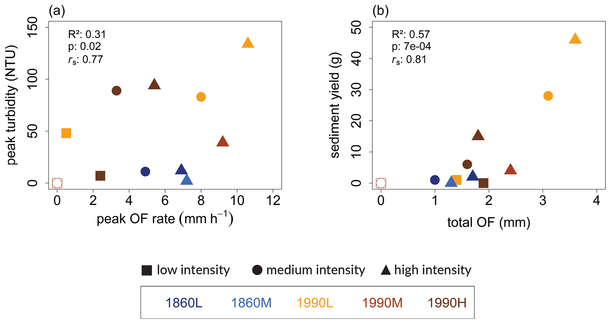
Figure 7 Scatterplots showing the relation between the peak OF rate and peak turbidity (a) and between total overland flow and sediment yield (b) for all sprinkling experiments on the five plots (1860L, 1860M, 1990L, 1990M, and 1990H). The color of the symbol represents the plot; the symbol represents the sprinkling experiment (low intensity, LI; medium intensity, MI; and high intensity, HI). The coefficient of determination (R²) and corresponding p value as well as the Spearman rank correlation coefficient (r_s) are given in the upper left-hand corner of each subplot. Note that no OF was measured (and, thus, the peak OF rate, peak turbidity, and total sediment yield were zero) for 5 of the 15 experiments, as indicated by the open symbols (only the result for the 1990H LI and MI experiments are visible because the data points plot on top of each other).

4.3 Sand movement

4.3.1 Patterns of sand movement and changes in sand-covered areas

Individual sand particles and small clusters of sand (< 1 cm²) were detected below the sand ribbon on both the 1860L and 1860M plots (Fig. 8). For the 1860L plot, sand movement was more widespread during the HI experiment (blue sand ribbon) than for the other experiments, as reflected by the larger areas covered by the sand for the HI experiment compared with the LI and MI experiments. Such large sand-covered areas were also observed for the 1990L and 1990M plots (Fig. 8). For the 1990H plot, individual sand particles, small clusters, and larger sand-covered areas were detected below the sand ribbons. However, compared to the 1990L and 1990M plots, hardly any sand moved on the 1990H plot. These qualitative differences in sand movement between the moraines are also reflected in the change in the sand transport distances ΔD (p= 3 × 10⁻³) and the change in the sand-covered areas ΔA (p= 2 × 10⁻³; Fig. 9, Table 2).

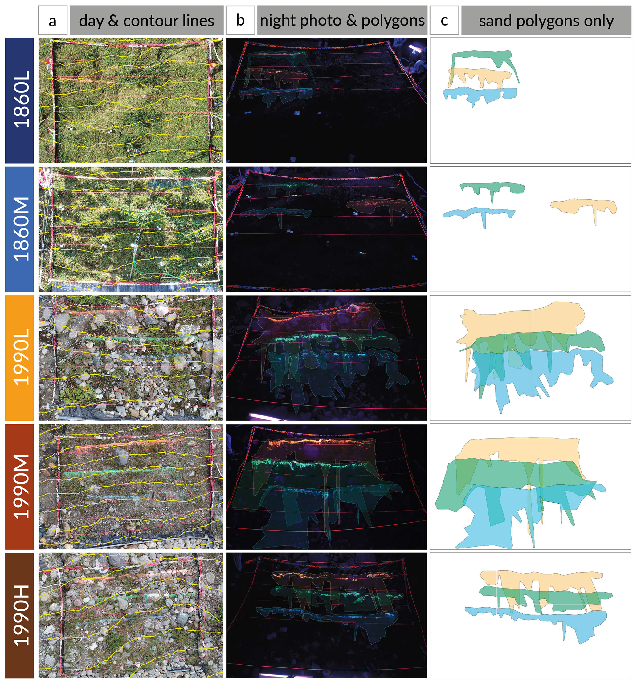
Figure 8 Photographs showing the sand-covered areas after the sprinkling experiments for the five plots. Panel (a) shows the daylight drone photos with the 50 cm contour lines (yellow lines). The orange sand ribbon was added prior to the low-intensity (LI) experiments, the green sand prior to the medium-intensity (MI) experiments, and the blue sand prior to the high-intensity (HI) experiments. Panel (b) shows the nighttime photos taken after the experiments, while illuminating the fluorescent sand with the UV lamps. To better visualize the extent of the sand movement, hand-drawn polygons (translucent orange – LI experiment; green – MI experiment; and blue – HI experiment) depicting the maximum extent of the individual sand particles and clusters were added to the photos. These polygons are also shown with a white background in panel (c). The larger sand-covered areas (and transport distances) for the 1990 plots compared with the 1860 plots are reflected by the larger polygons. The full-size version of the daylight photos with the contour lines and the night photos of the fluorescent sand (without polygons) are given in Figs. S1–S10 in the Supplement and are available in a higher resolution from Maier and van Meerveld (2023).

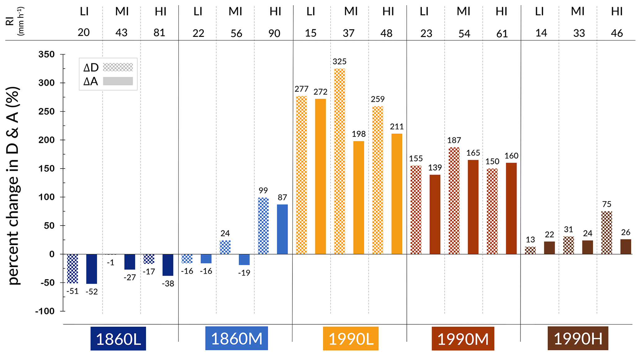
Figure 9 Change in the sand distance (ΔD; shaded bars) and sand-covered area (ΔA; solid bars) between the pre- and post-sprinkling conditions for all experiments on all five plots. LI, MI, and HI represent the low-, medium-, and high-intensity sprinkling experiments. Positive changes reflect increases in sand distances and areas during the experiment (and, thus, sand movement and deposition on the surface below the sand ribbon), whereas negative changes reflect a loss of sand from the surface (not an upward movement). The number above the plot denotes the rainfall intensity (RI; mm h⁻¹).

For five of the six experiments on the 1860 moraine, the change in sand-covered area was negative (i.e., the area covered with the fluorescent sand decreased during the experiment). The calculated sand transport distance was negative for four of the six experiments, also indicating the disappearance of the fluorescent sand (not upslope transport). Such decreases indicate that the sand moved and was washed into the soil or hidden below rocks or vegetation. This was not observed for the experiments on the 1990 moraine (Fig. 9). The decreases in ΔD and ΔA were largest for the LI experiment on the 1860L plot (ΔD of −51 % and ΔA of −52 %); the increases were largest for the 1990L plot (Fig. 9).

4.3.2 Comparison with the blue dye

The fluorescent sand and the blue dye on the 1990L plot were both transported to the bottom of the plots (Figs. 8, 10) and the flow pathways of the blue dye tracer matched the distribution of the sand-covered areas well (Fig. 10a, b). Sand and OF moved in four distinct areas, which matched the flow patterns derived from the DSM (Fig. 10c). The first flow path (no. 1 in Fig. 10) was located towards the left plot boundary (when looking upslope). The orange sand placed on the plot before the LI experiment was redistributed along this flow path. The second OF flow path (no. 2 in Fig. 10) was located further down and slightly to the left. Sand particles from all three sand ribbons were found here, suggesting that OF occurred here during all three experiments. The third pathway (no. 3 in Fig. 10) is mainly characterized by ponding in the slightly flatter area of the plot. In this microtopographic depression, the blue sand from the HI experiment was deposited. A fourth OF pathway (no. 4 in Fig. 10) was observed during all experiments, and all three sand colors were found in this area.

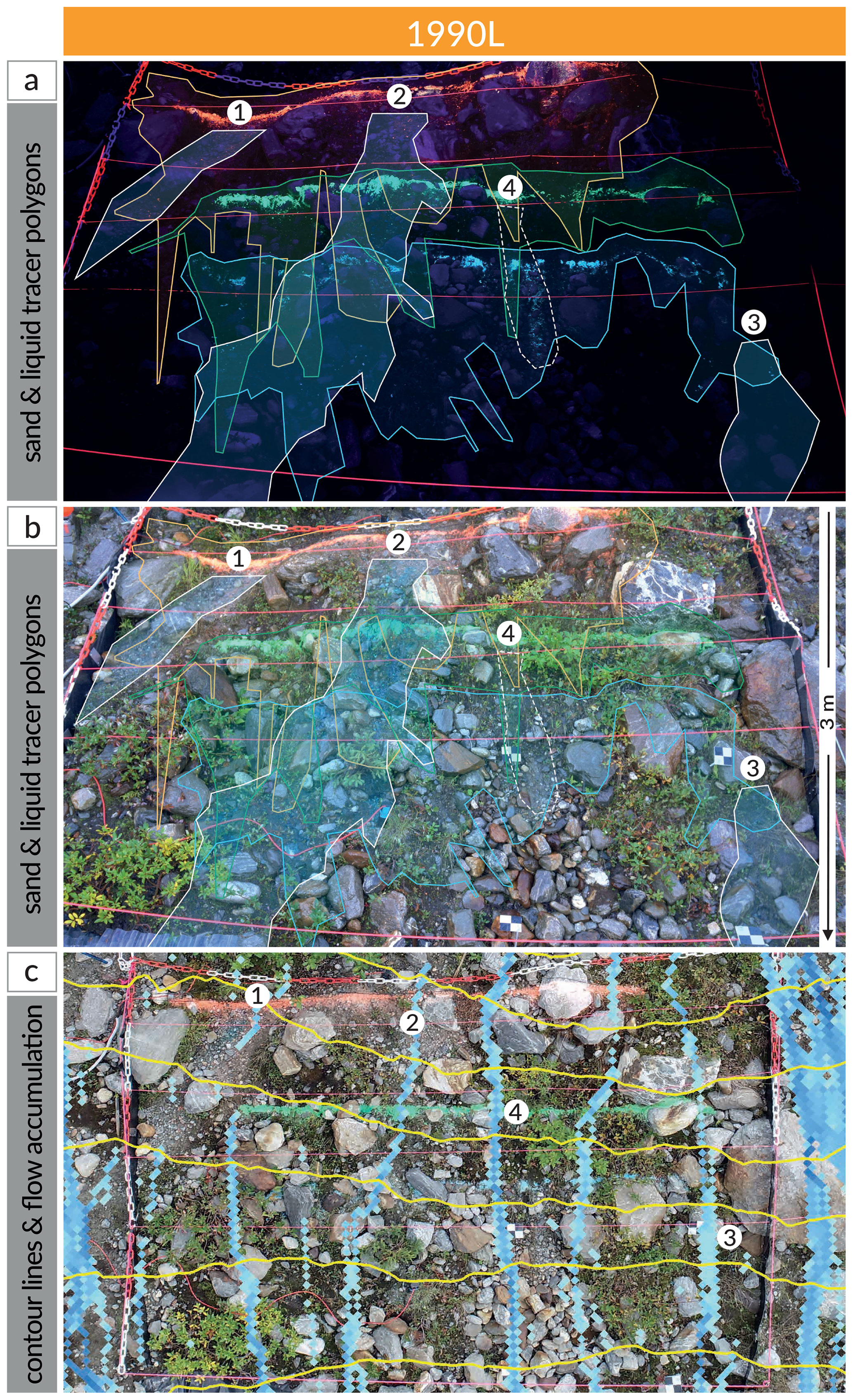
Figure 10 Overland flow (OF) pathways during the sprinkling experiments and sand-covered areas after the sprinkling experiments for the low-complexity plot on the 1990 moraine (1990L). Panel (a) was taken at night, and the hand-drawn orange, green, and blue polygons (from Fig. 8) were added to visualize the distribution of the fluorescent sand. The white polygons indicate OF pathways that were either clearly visible (no. 4) or traced by adding a brilliant blue tracer (no. 1, no. 2, and no. 3) to the water during the sprinkling. Numbers 1–4 reflect specific flow pathways that are described in the text. Panel (b) is a composite of several video frames from the MI and HI experiments after the addition of the blue dye to visualize the OF pathways on the plot, again with the polygons that visualize the distribution of the fluorescent sand. Panel (c) shows a nadir view of the plot surface and includes the 50 cm contour lines (yellow) and the D_∞-derived flow accumulation (values larger than 0.2 m² in blue).

4.4 Relation between overland flow, sand movement, and plot characteristics

There was no significant correlation between the percent changes in sand-covered area (ΔA) and either total OF (r_s= 0.51, p = 0.07), the OF runoff ratio (r_s= 0.52, p= 0.05), peak flow rate (r_s= 0.34, p= 0.40), peak turbidity (r_s= 0.52, p= 0.09), sediment yield (r_s= 0.56, p= 0.09), or sediment yield per unit rainfall (r_s= 0.58, p= 0.08; Fig. 11). This was mainly due to the fact that, for some experiments, no OF was measured at the bottom of the plot but there were changes in the sand-covered area. If these events are excluded from the analyses, a higher percent change in the sand-covered area corresponded to more OF, a higher OF runoff ratio, peak OF rate, peak turbidity, sediment yield, and sediment yield per unit rainfall (Fig. 11). Relations with the sand transport distance (ΔD) were similar to those for the change in sand-covered area (see Fig. S11).

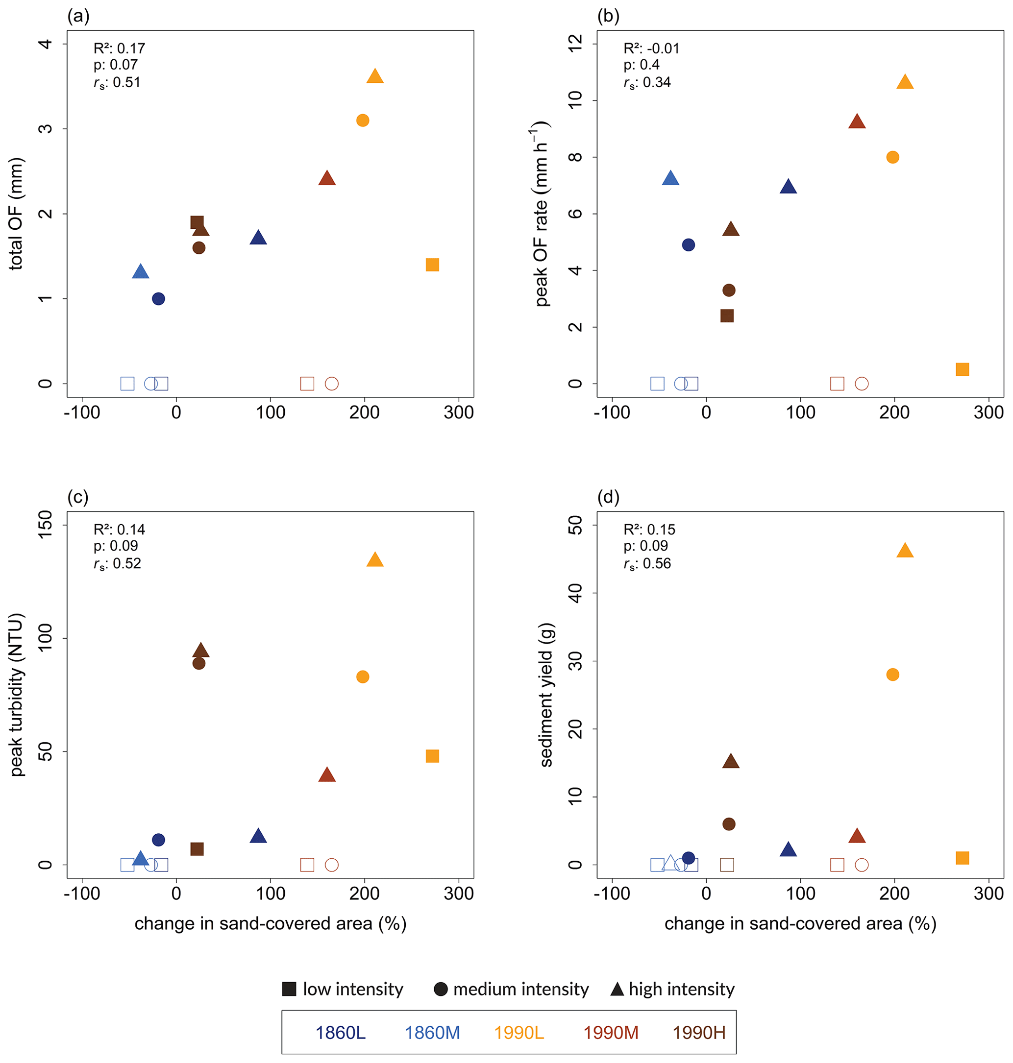
Figure 11 Scatterplots showing the relations between the change in (a) sand-covered area (ΔA) and total overland flow (OF), (b) ΔA and peak OF rate, (c) ΔA and peak turbidity, and (d) ΔA and total sediment yield for all sprinkling experiments. The color of the symbols represents the plots (1860L, 1860M, 1990L, 1990M, and 1990H); the symbol represents the rainfall intensity of the sprinkling experiment (LI, MI, and HI). Open symbols are used for experiments that did not generate any OF at the bottom of the plot (and, consequently, for which there is no turbidity measurement or sediment yield). The coefficient of determination (R²) and corresponding p value as well as the Spearman rank correlation coefficient (r_s) are given in the upper left-hand corner of each subplot. The results for ΔD are similar and are shown in Fig. S11 in the Supplement.

The percent change in sand-covered area (r_s= 0.77, p= 7 × 10⁻⁴; Fig. 12g), the OF runoff ratio (r_s= 0.78, p= 6 × 10⁻⁴; Fig. 12a), total OF (r_s= 0.66, p= 7 × 10⁻³), and sediment yield (r_s= 0.62, p= 0.01; Fig. 12d) were all significantly and positively correlated with the surface rock cover. The percent change in sand-covered area (r_s= 0.55, p= 0.03; Fig. 12i), OF runoff ratio (r_s= 0.54, p= 0.04; Fig. 12c), total OF (r_s = 0.54, p= 0.04), and rock cover (r_s= 0.53, p= 0.03) were also significantly and positively correlated with the surface roughness (i.e., tortuosity index). The percent change in sand-covered area was negatively correlated with the vegetation cover (r_s= −0.57, p= 0.03; Fig. 12h) and positively correlated with K_sat (r_s= 0.62, p= 0.02).

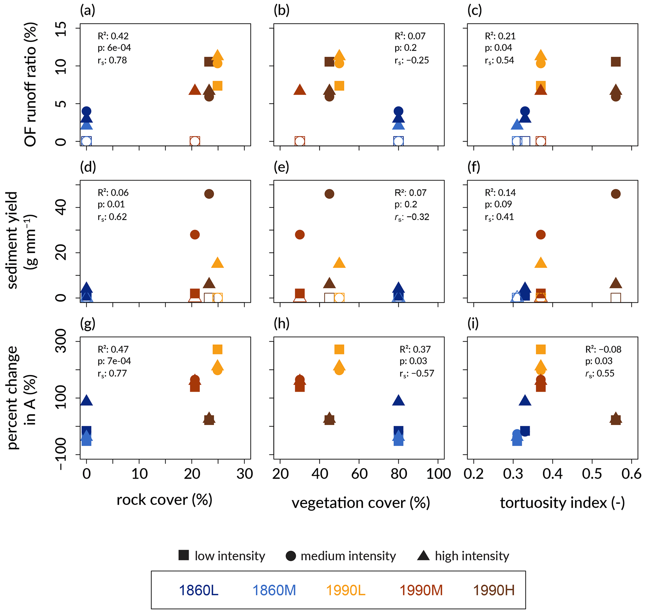
Figure 12 Scatterplots showing the relations of the OF runoff ratio (%), sediment yield per unit precipitation (g mm⁻¹), and percent change in sand-covered area (ΔA) with rock cover (%), vegetation cover (%), and the tortuosity index (−) for all sprinkling experiments. The color of the symbols represents the plots (1860L, 1860M, 1990L, 1990M, and 1990H); the symbol represents the rainfall intensity of the sprinkling experiment (LI, MI, and HI). Open symbols are used for experiments that did not generate any OF at the bottom of the plot (and, thus, no sediment yield). The coefficient of determination (R²) and corresponding p value as well as the Spearman rank correlation coefficient (r_s) are given in the upper left-hand and right-hand corner of each panel.

The multiple linear model indicated that rock cover, vegetation cover, and their interaction with the rainfall intensity could predict the total OF (R²= 0.64, root-mean-square error (RMSE) = 0.6 mm) and sediment yield (R²= 0.77, RMSE = 5.2 g) reasonably well, but these plot characteristics were not very suitable predictors of the percent change in sand-covered area (R²= 0.35, RMSE = 70 %).

5 Discussion

5.1 Advantages and disadvantages of fluorescent sand to study sediment transport

The results of this study suggest that fluorescent sand can be useful to assess sediment transport on natural hillslopes with coarse soils and little vegetation (Fig. 10). In particular, it provided information on the movement of particles on the plot. A main benefit of the sand tracer method is that very local and short sediment transport distances are identifiable. Thus, some information on OF and soil erosion can be obtained, even if no OF is detected below the plots. The distribution of the fluorescent sand particles matched that of the blue dye and provides information on OF infiltration and sediment deposition locations and, thus, on local deposition areas or sinks (e.g., pathway no. 3 in Fig. 10). For two experiments (LI and MI) on the 1990M plot, there was considerable sediment movement, although no OF was recorded. This sediment movement would not have been known if there were only measurements at the bottom of the plot (and also explains the lack of the correlation between sediment yield and sand movement; Fig. 11d). Thus, the movement of the sand highlighted the importance of OF re-infiltration on this plot. In other words, the fluorescent sand can help us to understand where sediment transport occurs and, thus, provides information about functional connectivity. The related disadvantage of the fluorescent sand method is that it only describes the local movement of fluorescent sand particles (i.e., plot-scale movement) and can not be used to predict sediment yield at the bottom of the plot. For sediment yield, the particles need to travel at least to the bottom of the plot, which was not the case for several of our experiments.

The fluorescent sand method is well suited to study sediment transport on poorly vegetated soils that contain a significant amount of sand (i.e., have a similar grain size to the sand tracer). In other words, it is well suited for studies on hillslopes in high alpine regions, dunes, etc. However, the sand does not move exactly like the soil. The fluorescent sand was loose and did not represent natural soil aggregates. On soils with finer-textured material, the method will no longer represent the detachment and transport of the natural soil particles.

The detection of the sand would have been possible without the use of the LED lamps or with a common fluorescent tracer without afterglow effect (as used by Hardy et al., 2019, 2017, 2016; Tauro et al., 2016, 2012a, b; Young and Holt, 1968). However, the use of a glow-in-the-dark sand that emits light for several minutes without a light source is a considerable advantage for rough surfaces, where vegetation or rocks lead to shading and some of the sand particles cannot be seen directly. By moving the LED and UV light sources around the plot before taking the photos, it was possible to see these particles due to their afterglow. On young moraines where the surface is rough, this is particularly useful.

An advantage of the fluorescent sand is that it can be used to study sediment transport during natural rainfall events (although we did not do this). Many of the previous studies that have described OF pathways required real-time observations of the water or the tracer. To automate data collection during the event, they measured water temperatures with thermal cameras (Lima et al., 2015) or recorded videos for particle detection on beaches, rivers, or hillslopes (Tauro et al., 2012a, b, 2016; Hardy et al., 2017, 2016). This requirement for photographs or videos during the event means that the tracer can only be used during sprinkling experiments or in places where the timing of sediment transport is predictable (e.g., on the beach). The advantage of the fluorescent sand method, as presented here, is that it does not require a real-time particle detection or tracking system. This means that the particles can, at least in theory, be applied to a surface and photographs can be taken before and after the rainfall event, so that natural conditions can be studied. This is especially useful in remote or exposed locations, when the occurrence of the next natural rainfall event is unknown, and where experiments need to be done on multiple plots simultaneously and it is too expensive to equip each plot with a camera. If equipment is available, real-time particle tracking has the advantage that it also provides information on when sediment transport occurs and can record the actual water flow.

The dissolution of the glue was a disadvantage of the fluorescent sand that we used. Despite being listed as waterproof, the sand formed aggregates (1–15 mm in size) after a wetting and drying cycle. The aggregates were rather stable, indicating that parts of the glue that bonded the photoluminescent powder to the sand particles dissolved during the sprinkling experiments and bound with other particles, mainly other (i.e., neighboring) fluorescent sand particles, after drying. In the following sprinkling experiments, such “glue-induced aggregates” were barely broken up and were, thus, unlikely to be transported (although there was still some transport). As a result, the fluorescent sand that we used can only be used to determine sediment transport for the first event after an application (as we did). This is a disadvantage because it requires application before the event of interest. The advantage is that there is more time to take the photographs after the event because the pattern will not change considerably due to a second event. Another type of fluorescent sand should be used to study sediment transport during multiple events. We did not observe washed off tracer powder on natural sand particles that would create “fake particles”. Also, no photo-quenching effects nor changes in the color were observed between the pre- and post-event photos. Even if there would have been small changes in the color, these would not have had an effect, as the typical color range for the sand was determined based on the pre- and post-experiment photos separately.

We consider the method used in this study applicable for microscale (several centimeters) to plot-scale (several meters) experiments but do not recommend its use for larger scales. First, the image resolution would become too coarse. With a modified setup, one could study sediment transport at larger scales, e.g., one could use the camera at different locations (to monitor different areas of the hillslope) and stitch the photos together or use a camera on a rail that takes several pictures of the hillslope. Second, on larger plots or longer hillslopes, the sand is more likely to get stuck behind rocks and vegetation, so that it is unlikely to be observed far from the applied ribbon. However, this provides interesting information to understand sediment transport distances and connectivity as well. A solution could be the use of multiple sand ribbons of different colors.

Another disadvantage of our approach was the movement and sagging of the fluorescent segmented chain as a reference marker. A solution would be the use of long and stable nails or markers with fluorescent tips that are anchored deep into the soil and, thus, represent more stable reference points. With more stable reference points, it would be possible to compare the pre- and post-event images more directly (although uncertainties in the georeferencing could also introduce errors here).

5.2 Effects of surface characteristics on overland flow and sand movement

The results of this study provide valuable information regarding OF generation and sediment transport on young moraines and how this changes during initial landscape development. However, these findings also need to be interpreted with caution, as the number of experiments and observations is very small. The significant differences in the total amount of OF and OF runoff ratios between the 1860 and 1990 moraines (Fig. 6) highlight the changes in the partitioning of rainfall into OF and infiltration (see also Maier et al., 2020) and sediment transport during landscape evolution. Vegetation cover (Greinwald et al., 2021a), root density (Greinwald et al., 2021b), and macroporosity (Hartmann et al., 2020a) increase during landscape evolution. The plots on the 1860 moraine were also characterized by a smoother surface than the 1990 moraine (Maier and van Meerveld, 2022) and were dominated by grassland vegetation with a dense root network and macropores close to the surface that promote infiltration (see Hino et al., 1987; Ding and Li, 2016; Greinwald et al., 2021b). On the plots on the 1860 moraine, most sand polygons were small and parts of the sand disappeared during the experiments (Figs. 8, 9; Table 2), which suggests vertical transport (translocation) of the sand particles (and water) into the macroporous topsoil or at least below the vegetation. The vegetation protects the soil particles from detachment (Geißler et al., 2012; Gyssels et al., 2005) and acts as a barrier that traps eroded sediment (Wainwright et al., 2000; Rey, 2003; Pearce et al., 1997; Marchamalo et al., 2016). The negative values for ΔD and ΔA for the plots on the 1860 moraine are, thus, mainly caused by the higher vegetation cover and macroporosity compared with the 1990 moraine (see Ebabu et al., 2018; Marques et al., 2007; Mu et al., 2019; Rey et al., 2004; Zhang et al., 2004).

The observed difference in total OF between the moraines and plots explains the difference in sediment yield (Figs. 6, 7b) and the redistribution of the fluorescent sand (Figs. 8, 10). The plot with the most OF also had the largest overall sediment yield (1990L). This is not surprising, as the importance of OF for soil erosion has been recognized for decades (e.g., Farmer, 1971; Knapen et al., 2007; Komura, 1976; Parsons, 1992; Poesen, 2017; Singer and Walker, 1983), even if other factors, such as the geotechnical properties of moraine sediments, also play an important role for slope stability, soil erosion, and sediment transport (Curry et al., 2009). The transport of the fluorescent sand below the ribbons (Fig. 8), however, also highlights that, even if no OF is measured at the bottom of the plot (Fig. 6), there may still be local OF and transport of sediment on the plot (Figs. 8, 9). Nonetheless, in these cases, connectivity to the bottom of the plot is low. Connectivity on larger scales (e.g., hillslope scale) may be even more different, as OF may infiltrate or exfiltrate as return flow, depending on downslope contributing areas and the connection of saturated areas along the flow paths (see, e.g., the analyses of Lane et al., 2004, 2009, based on the topographic wetness index, TWI).

The correlations between the surface characteristics and OF and sediment yield (Fig. 12) and the results of the multiple linear model suggest that the high rock cover and stone cover on the 1990 moraine led to considerable OF generation. Rock cover and sand content decrease with moraine age due to the effects of physical and chemical weathering (Musso et al., 2019, 2022; Maier et al., 2020). In alpine terrain, the effects of physical weathering due to congelifraction can be particularly fast. The rapid change in texture causes the K_sat to decrease during initial soil development, even though root density increases (Maier et al., 2020). However, in the areas covered with rocks (Fig. S12), infiltration is limited, leading to the generation of OF. Where this water infiltrates between the rocks, the sand particles are deposited on the surface or washed into the soil. This mainly occurred in the slightly flatter areas, behind vegetation patches, and behind rocks (e.g., flow path no. 3 in Fig. 10). Quicker and more pronounced OF responses on hillslopes with large rock cover and stone cover have been reported by others (e.g., Lavee and Poesen, 1991; Poesen et al., 1990; Poesen and Lavee, 1994). The positive, rather than negative, correlation between K_sat and sediment transport can be explained by the fact that K_sat was measured for the sediment between the rocks and not on the impermeable areas of the large rocks. The plot-average surface infiltration is much lower for the 1990 moraine than for the 1860 moraine due to the higher rock cover. The substantially higher OF on the 1990 moraine plots is also influenced by the position of the two plots at the footslope of the 1990 moraine, which caused the soils to be wetter and promoted saturated overland flow (Maier et al., 2021).

The rocks and stones on the 1990 moraine are also responsible for the higher surface roughness. A high surface roughness can reduce sediment connectivity and provide places where ponding occurs and OF infiltrates, and thus sinks for the sediment that it carries, preventing further downslope flow and transport (Thompson et al., 2010a; Dunkerley, 2003; Johnson et al., 1979; Jomaa et al., 2012). However, other studies (e.g., Darboux and Huang, 2005; Dunkerley, 2004; Helming et al., 1998) have reported a positive correlation between surface roughness, OF generation, and connectivity because surface roughness concentrates the flow and accelerates the flow of water in downslope-oriented structures. This flow can promote sediment transport and enhance erosion (Liu and Singh, 2004). We assume that this was the case for the plots of the 1990 moraine, where the OF pathways (as visualized by the blue dye) indeed followed microtopographic depressions with a downslope orientation (Fig. 10). The strong overlap between the redistribution of the fluorescent sand (sand polygons) and the pathways of the blue dye allowed the identification of the areas where OF occurred and where OF re-infiltrated (Fig. 10). However, the opposite is not true: a lack of sediment movement should not be interpreted as an absence of surface water flow. Water and sediment movement can be disconnected (e.g., where the transport capacity of the water is too low to move the sediment, where OF infiltrates into the soil and then exfiltrates again, or where splash erosion is important). Also, OF that is generated close to the gutters (and, thus, far below the sand ribbon) would not have caused any movement of the fluorescent sand. Furthermore, not all of the sand movement can be attributed to OF-driven soil erosion. The different patterns of sand movement (isolated small clusters, aggregates, or even single sand particles vs. more connected parts covered by fluorescent sand) indicate the influence of splash erosion. Recorded maximum splash distances for sand particles with a similar diameter to the fluorescent sand used in this study (300–500 µm) are ∼ 45 cm for rainfall intensities of ∼ 30 mm h⁻¹ and a median raindrop size of ∼ 1.4 mm (Legout et al., 2005), suggesting that some of the particles may have moved by splash erosion as well.

6 Conclusions

We tested the use of fluorescent sand with an afterglow in combination with sprinkling experiments to study sediment transport on young moraines in the Swiss Alps. Although fluorescent particles have been used in previous studies, in particular in flume experiments, this study highlights the potential of using fluorescent sand with an afterglow to identify and quantify sediment transport on natural hillslopes. The afterglow of the fluorescent sand improves the visibility of the sand on rough surfaces, such as hillslopes in proglacial areas. The main advantage of fluorescent sand as a tracer to study sediment movement is that it shows the redistribution of sediment on the plot, and thus provides information on sediment movement even if no OF is observed at the bottom of the plot. Another advantage is that the sand is cheap and that no photos or videos need to be taken during the experiment, making it logistically easier to study sediment transport during events on multiple plots.

The fluorescent sand was transported to distinct areas on the plots that matched the pathways of the OF during a blue dye staining experiment. The redistribution of the fluorescent sand also highlighted the differences in sediment transport processes for the two moraines. The more extensive vegetation cover on the older moraine protected the surface from splash detachment and transport and also promoted infiltration of OF and sediment into near-surface macropores and other preferential flow paths. In contrast, the high rock cover on the younger moraine led to concentrated OF pathways and larger sediment transport distances, and, for some experiments, a high sediment yield. These observations highlight the importance of microtopography for sediment transport and the importance of the re-infiltration of OF and deposition of sediment behind vegetation patches and rocks as well as the changes in sediment transport during the initial years of landscape evolution.