the Creative Commons Attribution 4.0 License.
the Creative Commons Attribution 4.0 License.
 | 14 Dec 2023
Towards robust seasonal streamflow forecasts in mountainous catchments: impact of calibration metric selection in hydrological modeling
Diego Araya
Eduardo Muñoz-Castro
James McPhee
Dynamical (i.e., model-based) methods are widely used by forecasting centers to generate seasonal streamflow forecasts, building upon process-based hydrological models that require parameter specification (i.e., calibration). Here, we investigate the extent to which the choice of calibration objective function affects the quality of seasonal (spring–summer) streamflow hindcasts produced with the traditional ensemble streamflow prediction (ESP) method and explore connections between hindcast skill and hydrological consistency – measured in terms of biases in hydrological signatures – obtained from the model parameter sets. To this end, we calibrate three popular conceptual rainfall-runoff models (GR4J, TUW, and Sacramento) using 12 different objective functions, including seasonal metrics that emphasize errors during the snowmelt period, and produce hindcasts for five initialization times over a 33-year period (April 1987–March 2020) in 22 mountain catchments that span diverse hydroclimatic conditions along the semiarid Andes Cordillera (28–37∘ S). The results show that the choice of calibration metric becomes relevant as the winter (snow accumulation) season begins (i.e., 1 July), enhancing inter-basin differences in hindcast skill as initializations approach the beginning of the snowmelt season (i.e., 1 September). The comparison of seasonal hindcasts shows that the hydrological consistency – quantified here through biases in streamflow signatures – obtained with some calibration metrics (e.g., Split KGE (Kling–Gupta efficiency), which gives equal weight to each water year in the calibration time series) does not ensure satisfactory seasonal ESP forecasts and that the metrics that provide skillful ESP forecasts (e.g., VE-Sep, which quantifies seasonal volume errors) do not necessarily yield hydrologically consistent model simulations. Among the options explored here, an objective function that combines the Kling–Gupta efficiency (KGE) and the Nash–Sutcliffe efficiency (NSE) with flows in log space provides the best compromise between hydrologically consistent simulations and hindcast performance. Finally, the choice of calibration metric generally affects the magnitude, rather than the sign, of correlations between hindcast quality attributes and catchment descriptors, the baseflow index and interannual runoff variability being the best predictors of forecast skill. Overall, this study highlights the need for careful parameter estimation strategies in the forecasting production chain to generate skillful forecasts from hydrologically consistent simulations and draw robust conclusions on streamflow predictability.
- Article
(5644 KB) - Full-text XML
-
Supplement
(3004 KB) - BibTeX
- EndNote


Seasonal streamflow forecasts can support long-term water resources management and planning, including allocations for water supply, irrigation, hydropower generation, industry, mining operations, and navigation. Therefore, improving the quality of these products is an ongoing challenge for the hydrology community, especially in regions where drought risk and severity are expected to increase under climate change scenarios (Cook et al., 2022). Among the existing approaches, dynamical methods – which rely on the implementation of hydrological or land surface models (Wood et al., 2018; Slater et al., 2023) – are attractive because they involve explicit hydrologic process representations, with varying degrees of abstraction depending on model complexity (Hrachowitz and Clark, 2017). Accordingly, dynamical systems not only offer the opportunity to monitor and predict other variables than streamflow (e.g., Singla et al., 2012; Greuell et al., 2019) but also provide mechanistic explanations for the current and future state of hydrological systems.
In particular, the ensemble streamflow prediction (ESP; Day, 1985) technique has been used operationally by many forecasting agencies in the world and is considered a baseline for the implementation of dynamical forecasting frameworks (Wood et al., 2018). The approach relies on historical sequences of climate time series forcing a hydrology or land surface model for a given forecast initialization time. Because of its simplicity and relatively low cost, ESP has been widely used as a reference for developing and testing more complex forecasting frameworks that incorporate dynamical climate model outputs to force hydrologic model simulations (e.g., Yuan et al., 2014; Arnal et al., 2018; Lucatero et al., 2018; Wanders et al., 2019; Peñuela et al., 2020; Baker et al., 2021). Notably, the approach remains a hard-to-beat benchmark when the target predictand is spring–summer snowmelt runoff (e.g., Arnal et al., 2018; Wanders et al., 2019), since it was originally designed to provide more skill for regions and times in the year where initial hydrologic conditions (IHCs) dominate the seasonal hydrologic response. This has motivated a large body of research to improve ESP forecasts in snow-dominated areas, including verification and diagnostics of operational systems (e.g., Franz et al., 2003), the implementation of data assimilation methods (e.g., DeChant and Moradkhani, 2014; Micheletty et al., 2021), climate input selection (i.e., pre-ESP; Werner et al., 2004), statistical post-processing techniques (e.g., Wood and Schaake, 2008; Mendoza et al., 2017), and multi-model combination strategies (e.g., Bohn et al., 2010; Najafi and Moradkhani, 2015).
However, and despite the reliance of dynamical and some types of hybrid (i.e., statistical-dynamical; see review by Slater et al., 2023) approaches on hydrologic models, there has been limited attention on how parameter estimation strategies may affect seasonal forecast quality. In particular, the choice of calibration metric is crucial because it involves defining the processes and/or target variables (including streamflow characteristics) that need to be well simulated for specific water resources applications (e.g., Pool et al., 2017; Mizukami et al., 2019).
In seasonal streamflow forecasting, the Nash–Sutcliffe efficiency (NSE; Nash and Sutcliffe, 1970) – a normalized version of the mean-square error – is a common choice for single-objective (e.g., Giuliani et al., 2020; Sabzipour et al., 2021) or multi-objective (e.g., Shi et al., 2008; Bohn et al., 2010) calibration frameworks. Other studies have preferred related metrics, like the mean-square error (e.g., DeChant and Moradkhani, 2014), the root-mean-square error (e.g., Huang et al., 2017), and the mean absolute error (e.g., Yuan et al., 2013) between observed and simulated streamflow. Another popular choice is the Kling–Gupta efficiency (KGE; Gupta et al., 2009), which has been applied to raw streamflow (e.g., Micheletty et al., 2021), root-squared flows (e.g., Crochemore et al., 2016; Harrigan et al., 2018), and inverse flows to emphasize low streamflow (Crochemore et al., 2017). The KGE has also been used in its non-parametric form (Pool et al., 2018) to capture different parts of the hydrograph (Donegan et al., 2021), or it has been combined with NSE (e.g., Girons Lopez et al., 2021). Finally, seasonally oriented metrics are attractive if the aim is to constrain the calibration process to the time window of interest. For example, Yang et al. (2014) showed that calibrating hydrological model parameters using only data from the dry season improved forecast skill for months included therein in comparison to using the entire time series.
To the best of our knowledge, no previous studies have conducted a systematic assessment on how different types of calibration OFs may impact forecast quality attributes and their relationship with catchment characteristics. Even more, it remains unclear whether “good” seasonal forecasts are associated with calibration metrics that enable the main features of observed catchment behavior (i.e., hydrological consistency; Martinez and Gupta, 2010) to be reproduced. This is a critical issue if hydrological models need to be operationally implemented for multiple purposes, since traditional objective functions may not necessarily reproduce streamflow characteristics described with different mathematical formulations (e.g., Mendoza et al., 2015). Therefore, we address the following research questions:
-
How dependent is the quality of seasonal streamflow forecasts on the choice of calibration metric and forecast initialization times?
-
Is it possible to obtain skillful and reliable seasonal forecasts from hydrologically consistent simulations through an appropriate choice of calibration objective function?
-
How does the relationship between catchment characteristics and seasonal forecast quality vary for different calibration metrics?
To address these questions, we assess seasonal streamflow hindcasts produced with the ESP method, using three popular conceptual rainfall-runoff models calibrated with metrics that belong to different families of objective functions. We conduct our analyses over a collection of headwater basins in central Chile, where snow plays a key role in the hydrologic cycle (Mendoza et al., 2020; Murillo et al., 2022) and, especially, for streamflow predictability (Mendoza et al., 2014; Cornwell et al., 2016). Current operational practice in this region considers September–March (i.e., Spring and Summer) water supply forecasts produced only once a year (1 September), based on subjectively adjusted outputs from statistical models that regress streamflow volumes against in situ measurements of precipitation, temperature, snow water equivalent (SWE), and antecedent streamflow, among other variables (DGA, 2022). Hence, this paper provides a baseline for ongoing and future streamflow forecasting efforts using dynamical and/or hybrid methods in central Chile. Additionally, the selected basins cover a wide range of physiographic and hydroclimatic characteristics (Vásquez et al., 2021; Sepúlveda et al., 2022), enabling the examination of possible connections between forecast quality and catchment attributes (e.g., Harrigan et al., 2018; Pechlivanidis et al., 2020; Donegan et al., 2021).
We focus on 22 case study basins located in central Chile (28–37∘ S, 70–71∘ W), a domain that encompasses more than 60 % of the country's population and, therefore, many socioeconomic activities that depend on water availability. The selected basins are included in the CAMELS-CL dataset (Alvarez-Garreton et al., 2018) and meet the following criteria: (i) a low (i.e., <0.05) human intervention index, which is defined as the ratio between annual volume of water assigned for permanent consumptive uses and the observed mean annual runoff; (ii) absence of large reservoirs; (iii) no major consumptive water withdrawals from the stream; (iv) snowmelt influence on runoff seasonality (i.e., they must have a snowmelt-driven, nivo-pluvial, or pluvio-nival regime, as described by Baez-Villanueva et al., 2021); (v) at least 75 % of days with streamflow observations during the period April 1987–March 2020; and (vi) at least 20 water years (WYs) with seasonal (September–March) streamflow observations for hindcast verification purposes. The most restrictive conditions are (v) and (vi), which hinder the possibility to include additional mountainous catchments from CAMELS-CL; nevertheless, we consider that both requirements are essential for proper hydrologic model calibration and evaluation (since seasonal objective functions rely solely on Sep–Mar data availability) and a robust verification of seasonal streamflow hindcasts.
We use daily time series of observed streamflow and basin-averaged precipitation, mean air temperature, and potential evapotranspiration (PET) retrieved from the CAMELS-CL database (Alvarez-Garreton et al., 2018), which compiles information from different sources: (i) streamflow observations acquired from stations maintained by the Chilean General Water Directorate (DGA), also available on the DGA's website (https://dga.mop.gob.cl/, last access: 11 March 2023); (ii) basin-averaged precipitation and mean temperature data for the period 1979–2020, derived from the gridded observational product CR2MET (DGA, 2017; Boisier et al., 2018) version 2.0, which provides information of these variables for continental Chile at a horizontal resolution; and (iii) PET calculated with the formula proposed by Hargreaves and Samani (1985) using basin-averaged temperature from CR2MET. Additionally, elevation data from the ASTER Global Digital Elevation Model (DEM), version 3.0 (US/Japan Aster Science Team), is used to generate hypsometric curves for the basins.
Figure 1 shows a suite of attributes for our case study basins, whose mean elevations and areas range between 1605–4275 m a.s.l. and 81–4839 km2, respectively. The selected basins provide a pronounced hydroclimatic gradient, with aridity indices – defined as the ratio between mean annual potential evapotranspiration (PET) and mean annual precipitation (P) – spanning 0.5–7.0. Indeed, there is a north–south transition from semi-arid, water-limited hydroclimates (with PET) towards energy-limited environments (with PET; see Figs. 1c and 2d), with larger precipitation and runoff amounts. No clear spatial patterns are found in the fraction of precipitation falling as snow. The catchment attribute values are provided in Table S1 (in the Supplement), including precipitation seasonality, baseflow index, and other characteristics.
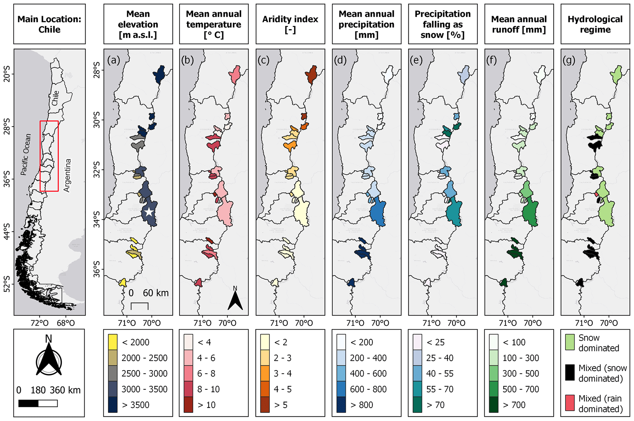
Figure 1Location and spatial variability of catchment characteristics across the study domain: (a) mean elevation, (b) mean annual temperature, (c) aridity index, (d) mean annual precipitation, (e) precipitation falling as snow, (f) mean annual runoff, and (g) hydrological regime. Hydroclimatic attributes are computed for the period April 1987–May 2020 using data retrieved from the CAMELS-CL database (see details in Sect. 2). The white star in panel (a) denotes the outlet of the Maipo en El Manzano River basin, for which the analysis approach is illustrated (see Sect. 4.1).
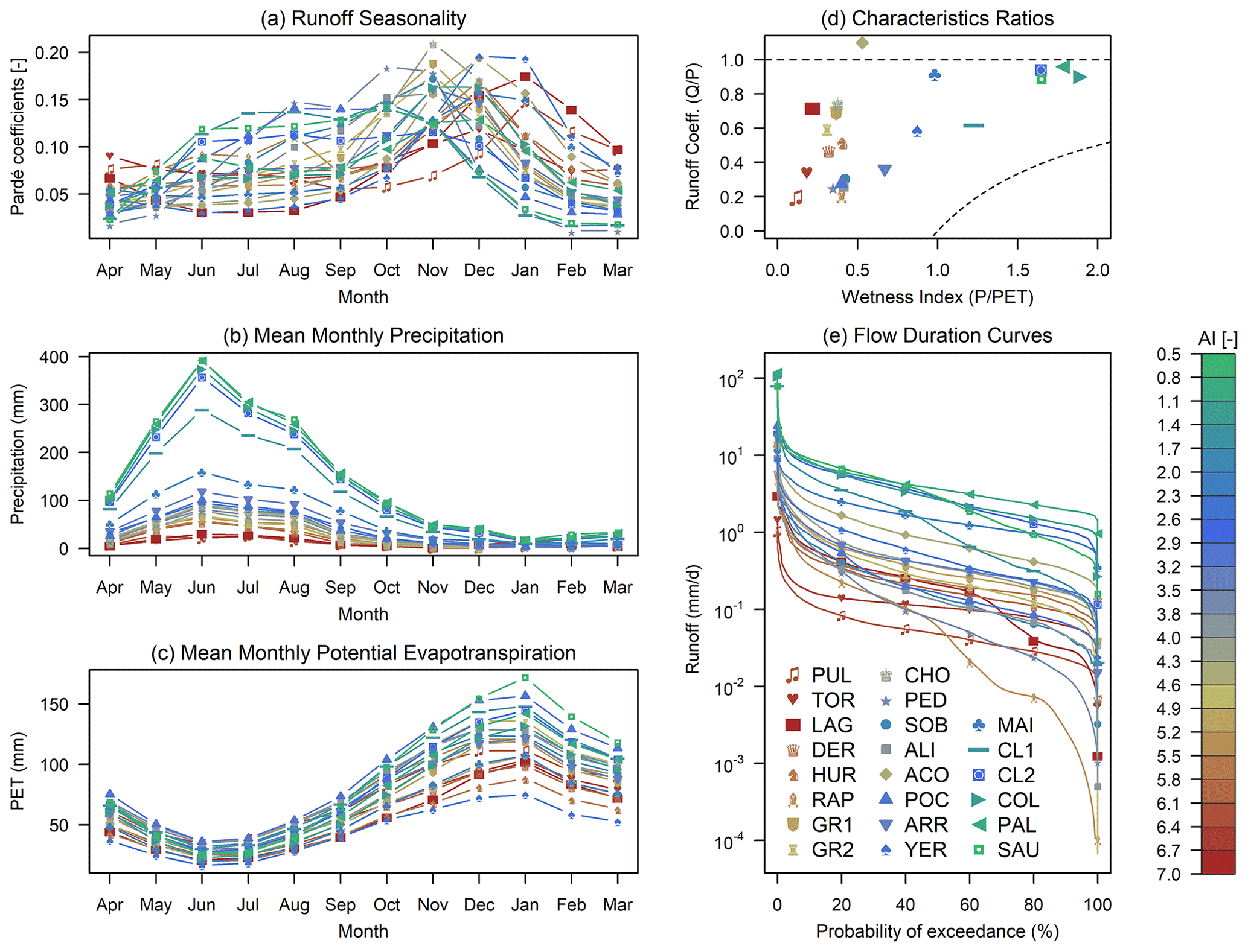
Figure 2Study basins' characteristics: (a) runoff seasonality, (b) mean monthly precipitation, (c) mean monthly potential evapotranspiration, (d) characteristic ratios, and (e) daily flow duration curves (FDC). These graphs correspond to the period April 1987–March 2020 and were produced using data retrieved from the CAMELS-CL database (see details in Sect. 2). In the legend (panel e), the basins are ordered from north (PUL) to south (SAU), and the colors indicate their aridity indices (AI; green to red – lower to higher index).
Figure 2 includes additional hydrological features for our sample of catchments. In terms of average seasonal patterns, higher Pardé coefficients are obtained in most basins during the snowmelt season (September–March, which spans the spring and summer seasons). Precipitation (Fig. 2b) is concentrated between April and September, and intra-annual variations in PET (Fig. 2c) are consistent with seasonal temperature fluctuations in central Chile (not shown). Figure 2d also shows that the case study basins span different annual water and energy balances, complementing the latitudinal gradients shown in Fig. 1. Aconcagua at Chacabuquito (ACO) is the only basin with a mean annual runoff ratio larger than 1, which can be explained by (i) underestimation of precipitation from CR2MET v2.0 or from meteorological station records used to develop the gridded product, (ii) positive biases in streamflow records from the DGA's stations due to uncertainties in stage–discharge relationships, or (iii) glacier and/or groundwater contributions. Finally, the daily flow duration curves (FDCs; Fig. 2e) show the diversity of hydrological responses, with differences in high/low flows, mid-segment slope, median, and other signatures.
In this paper, we use the term forecast when referring to past studies and applications at locations where observational data will not be available and to reflect on the implications of our results for operational practice. We use the term hindcast when referring to retrospective forecasts produced in this study, the term evaluation for the assessment of streamflow model simulations outside the calibration period, and verification for the assessment of seasonal streamflow hindcasts.
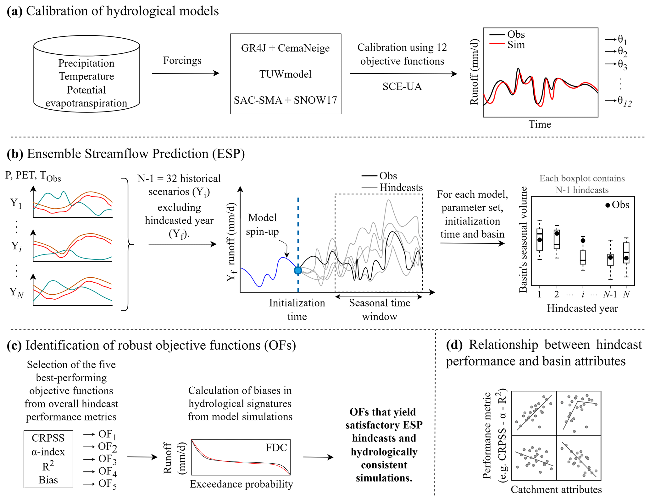
Figure 3 outlines our methodology, which includes four steps: (a) parameter calibration of three hydrological models (GR4J, TUW, and SAC-SMA) configured in 22 snow-influenced basins using a suite of 12 objective functions, (b) seasonal (September-March) streamflow hindcast generation with the ESP method for 33 WYs (April 1987–March 2020) and five initialization times and verification of forecast quality attributes, (c) assessment of hydrological consistency through five streamflow signatures for the subset of best-performing objective functions in terms of hindcast attributes, and (d) analysis of possible relationships between catchment characteristics and ESP hindcast attributes.
3.1 Hydrological modeling
3.1.1 Models
We use three conceptual, bucket-style hydrological models: (i) GR4J (Perrin et al., 2003) coupled with the CemaNeige snow module (Valéry et al., 2014b); (ii) the TUW model (Parajka et al., 2007), which follows the structure of HBV (Bergström, 1976); and (iii) the Sacramento Soil Moisture Accounting (SAC-SMA; Burnash et al., 1973) model combined with SNOW-17 (Anderson, 1973) and a routing scheme (Lohmann et al., 1996). These model structures were selected because they are widely used by the hydrology community (Addor and Melsen, 2019), with a myriad of applications to streamflow forecasting. For example, SAC-SMA has been applied for testing alternative approaches (e.g., Mendoza et al., 2017) and is used to produce operational streamflow forecasts in the United States (Micheletty et al., 2021). GR4J has been applied to assess streamflow forecasting frameworks in large samples of catchments (e.g., Harrigan et al., 2018; Woldemeskel et al., 2018). HBV-like conceptual models have been used to assess short-range (e.g., Pauwels and De Lannoy, 2009; Verkade et al., 2013) to long-range (e.g., Peñuela et al., 2020) streamflow forecasts, especially in European countries.
The GR4J model (Perrin et al., 2003) has a parsimonious structure consisting in two interconnected reservoirs and four free parameters. The CemaNeige module first partitions total precipitation into liquid and solid and then simulates snow accumulation and melt over five or more (user-defined; here we use 10) elevation bands, using a two-parameter degree-day-based scheme (Valéry et al., 2014b) that adds snowmelt and liquid precipitation to the soil-moisture-accounting reservoir. Water that is not intercepted or evaporated from the soil moisture accounting reservoir is partitioned into two fluxes: one is routed with a unit hydrograph and then by a nonlinear routing store, and the other is routed using a single unit hydrograph. A groundwater exchange term acts on both flow components to represent water exchanges between topographical catchments.
The TUW model consists of four main routines. In the snow routine (with five free parameters), precipitation is partitioned into snowfall and rainfall, and snow accumulation and melting are calculated with a degree-day scheme. Rainfall and snowmelt are inputs for the soil moisture routine (with three free parameters), which computes actual ET, soil moisture, and runoff heading to the response routine. With five free parameters, the response routing has an upper reservoir that produces surface runoff and interflow and a lower reservoir producing baseflow. Finally, a routing scheme (two free parameters) delays total runoff using a triangular transfer function.
The SAC-SMA (Burnash et al., 1973) has a more complex structure than the GR4J and TUW models (with 16 free parameters), dividing the catchment into (1) an upper zone that simulates hydrological processes occurring in the root, surface, and atmospheric zones, producing surface and direct runoff, and (2) a lower zone, where percolation occurs and baseflow is produced. The model is coupled with the conceptual snow accumulation and ablation model SNOW-17 (Anderson, 1973), which simulates snow accumulation and melt using a simplified energy balance and requires the specification of 10 free parameters. An independent, two-parameter routing scheme, based on the linearized Saint-Venant equation, is used to route runoff and baseflow (Lohmann et al., 1996).
Here, we use model versions from open-source packages implemented in the R statistical software (http://www.r-project.org/, last access: 5 January 2023). GR4J and CemaNeige (hereafter referred to as GR4J) are implemented in the open-source package “airGR” (Coron et al., 2017), whereas the TUW and SAC models are available in the packages “TUWmodel” (Viglione and Parajka, 2020) and “sacsmaR” (Taner, 2019), respectively. All the models require daily time series of catchment-scale precipitation (P; mm), PET (mm), and mean air temperature (T; ∘C). While the CemaNeige is configured with 10 elevation bands, the snow routines of the TUW and SAC-SMA models (i.e., SNOW-17) are implemented in a lumped fashion because preliminary experiments with these models showed that the benefits of adding snow bands on the KGE of daily flows were marginal. We stress that the use of three models does not seek to provide comparisons among different model structures; instead, we aim to examine to what degree our results and conclusions can be model-dependent.
3.1.2 Calibration strategy
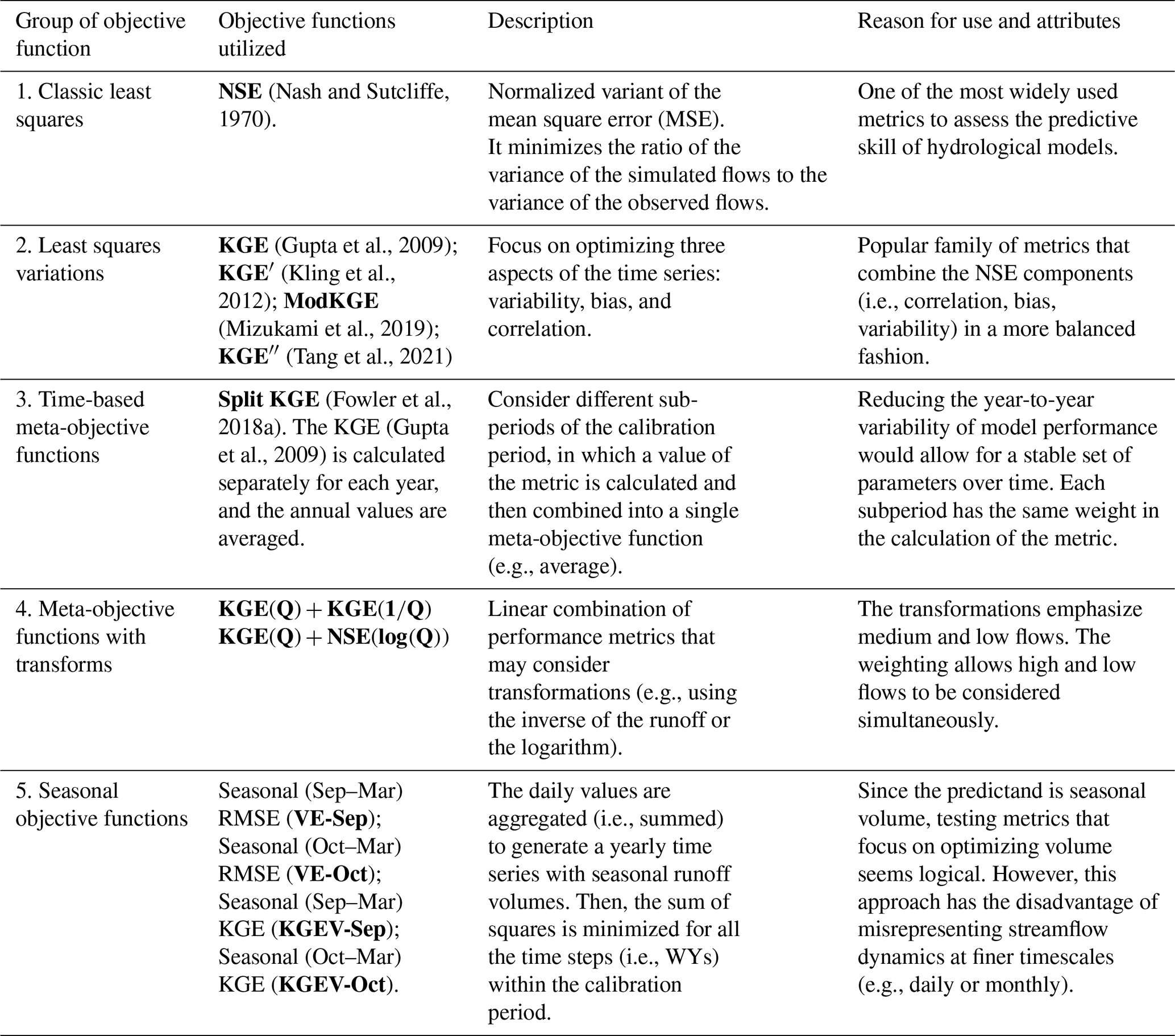
We calibrate model parameters (Fig. 3a) using the global optimization algorithm Shuffled Complex Evolution (SCE-UA; Duan et al., 1992), implemented in the R package “rtop” (Skøien et al., 2014). To compute the calibration objective function, we use modeled and observed streamflow data from the period April 1994–March 2013 because they span a diverse range of hydroclimatic conditions, considering the period April 1986–March 1994 for model spin-up. For each model and basin, we perform 12 calibrations using the objective functions listed in Table 1. Eight metrics (groups 1–4) are selected because they are representative of different families of objective functions and have been widely used for various modeling purposes. For example, the NSE with flows in log space (Log-NSE) has been used to enhance low-flow simulations (e.g., Oudin et al., 2008; Melsen et al., 2019), while the recently proposed Split KGE (Fowler et al., 2018a) aims to provide robust streamflow simulations under contrasting climatic conditions. Additionally, we include four calibration metrics formulated to improve seasonal streamflow simulations. Model evaluation is conducted by computing performance metrics with data from two periods: (i) April 1987–March 1994, which is hydroclimatically diverse, and (ii) April 2013–March 2020, which is characterized by unprecedented and temporally persistent dry conditions (Garreaud et al., 2017, 2019). To produce runoff simulations for each period, the preceding 8 years (i.e., April 1979–March 1987 and April 2005–March 2013) was used for model spin-up.
Table 1Objective functions used for model calibration. The bold text indicates the notation used in this paper.
3.2 Hindcast generation and verification
We produce seasonal streamflow hindcasts by retrospectively applying the ensemble streamflow prediction (ESP; Day, 1985) method. The approach relies on deterministic hydrologic model simulations forced with historical meteorological inputs up to the forecast initialization time, assuming that meteorological data and the model are perfect, which yields IHCs without errors. Then, the model is forced with an ensemble of climate sequences, attributing all the streamflow forecast uncertainty to the spread of future meteorological forcings (FMFs). In the traditional ESP implementation, each climate sequence (i.e., ensemble member) is drawn from a 1-year-observed meteorological time series, and the meteorological input traces associated with target years are excluded for hindcast generation/verification (Mendoza et al., 2017). Importantly, ESP cannot forecast extreme events with magnitudes that have not been recorded (Sabzipour et al., 2021), and forecast quality can be limited in non-stationary climates (Peñuela et al., 2020). Here, we apply the ESP method for the period April 1987–March 2020 (Fig. 3b), using five initialization times (from 1 May to 1 September). Hence, for each combination of catchment, hydrological model, parameter set (i.e., objective function), and initialization time, we complete the following steps:
-
Force model simulations during the eight WYs preceding the initialization time ti to obtain the initial hydrologic conditions (IHCs).
-
Using the states obtained in step 1, run hydrologic model simulations using observed meteorological data from the remaining 32 WYs (i.e., the forcings of the year to be hindcasted are not used), generating an ensemble of 32 traces for year n.
-
Aggregate daily streamflow volumes within the period of interest (1 September–31 March), obtaining an ensemble of 32 seasonal streamflow hindcasts.
Table 2Performance metrics used for seasonal streamflow hindcast verification.
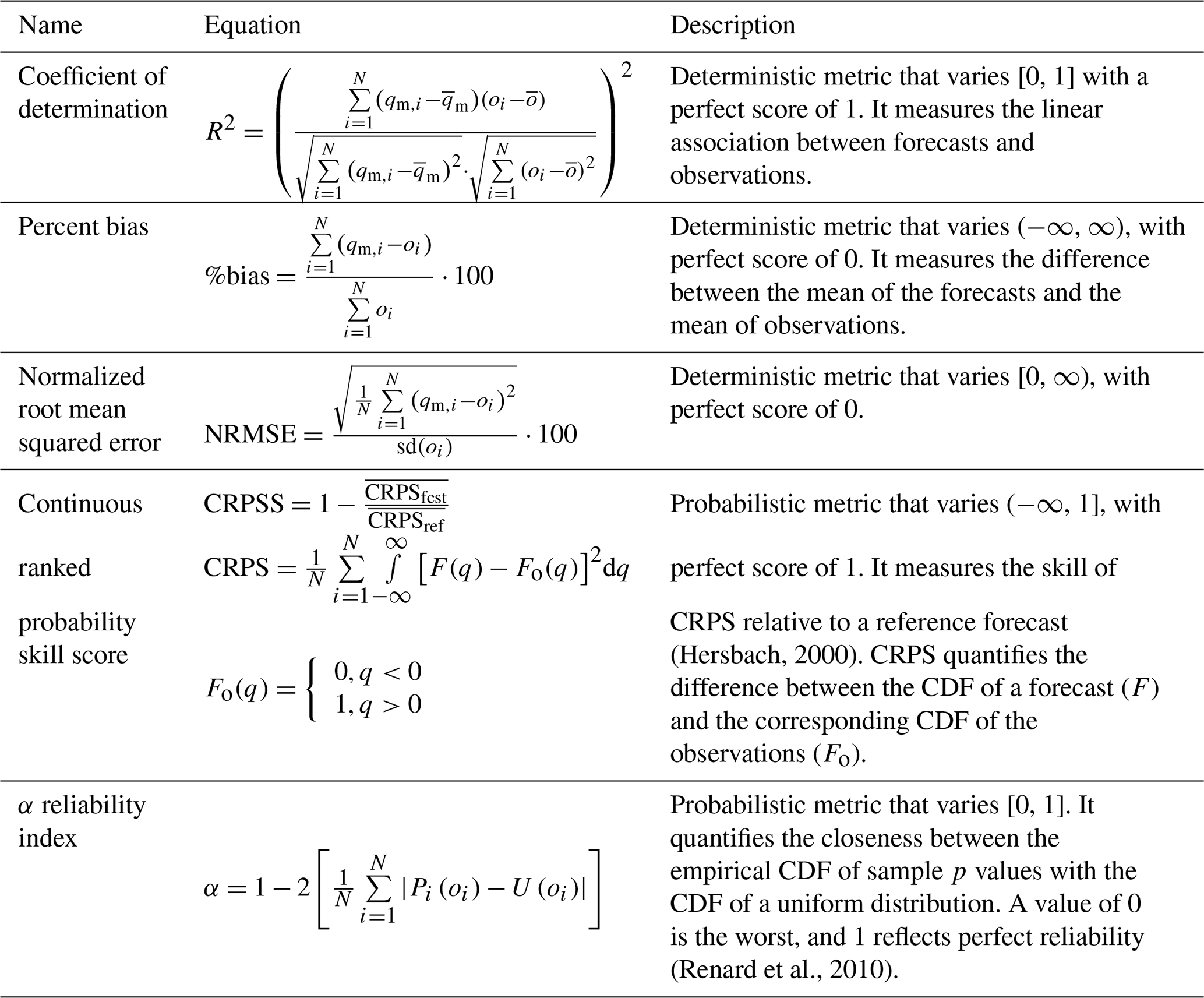
qm,i: forecast ensemble median for year i. : average over forecast ensemble medians. oi: observation for year i. average of observations. Pi(oi): non-exceedance probability of oi using ensemble forecast for year i. U(oi): non-exceedance probability of oi using the uniform distribution U [0, 1].
Steps 1–3 are repeated until a time series of 33 ensemble seasonal streamflow hindcasts is obtained. Then, we verify different hindcast quality attributes using a set of deterministic and probabilistic metrics (Table 2). These include standard measures such as the coefficient of determination (R2), the percent bias, and the normalized root mean squared error (NRMSE). All deterministic metrics are calculated using the ensemble median. Probabilistic skill is assessed through the continuous ranked probability score (CRPS; Hersbach, 2000), which measures the temporal average error between the forecast cumulative distribution function (CDF) and that from the observation. We compute the continuous ranked probability skill score (CRPSS) using the observed mean climatology as the reference forecast, instead of modeled data as in other studies (e.g., Harrigan et al., 2018; Crochemore et al., 2020), making our verification results independent from the choice of objective function and hydrological model. Forecast reliability – i.e., adequacy of the forecast ensemble spread to represent the uncertainty in observations – is assessed using the α index from the predictive quantile–quantile (QQ) plot (Renard et al., 2010). QQ plots compare the empirical CDF of forecast p values (i.e. Pi(oi), where Pi and oi are the forecast CDF and observation at year i) with that from a uniform distribution U[0, 1] (Laio and Tamea, 2007). All the hindcast verification metrics are calculated using the entire time series (i.e., 33 WYs).
Table 3Hydrological signatures used to evaluate the models' capability to generate hydrologically consistent simulations.
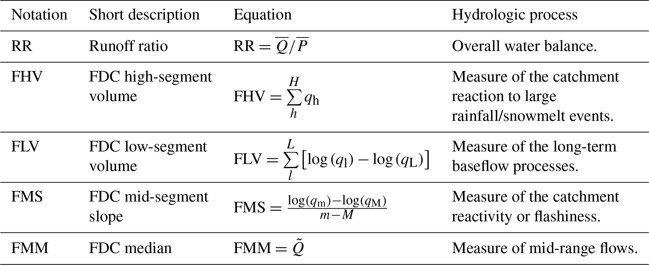
: average of a basin's runoff time series (Q). : average of a basin's precipitation time series (P). : runoff median value. qi: runoff observation/simulation for day i. qh: runoff observation/simulation for flows with exceedance probabilities lower than 0.02 in the FDC. ql: runoff observation/simulation for flows with exceedance probabilities greater than 0.70 in the FDC. qL: minimum runoff observation/simulation. qm: runoff observation/simulation with exceedance probability of 0.20. qM: runoff observation/simulation with exceedance probability of 0.70.
3.3 Assessment of hydrological consistency
From each family of objective functions listed in Table 1, we choose the one providing the overall best hindcast performance (quantified through the median from the sample of catchments) for all combinations of initialization time, performance metric, and model and evaluate its capability to provide hydrologically consistent simulations (Fig. 3c) using five signature measures of hydrological behavior. Our goal here is to explore the extent to which the quality of seasonal streamflow hindcasts – achieved with a specific calibration objective function – is connected to the model's capability to reproduce streamflow characteristics. Hence, we select metrics that cover various aspects of simulated catchment response, including precipitation partitioning into ET and runoff, high- and low-flow volumes, flashiness of runoff and medium flows. The notation, short description, mathematical formulation, and physical process associated with each streamflow signature are detailed in Table 3.
We also examine possible variations (gain/loss) in hindcast skill when selecting a popular (i.e., NSE) or alternative objective functions (OFs) that yield hydrologically consistent model simulations (CRPSSOF), relative to reference forecasts obtained with the overall best objective function in terms of hindcast performance (CRPSSREF):
Here, we use Eq. (1) for hindcasts initialized on 1 September.
3.4 Drivers of seasonal streamflow predictability
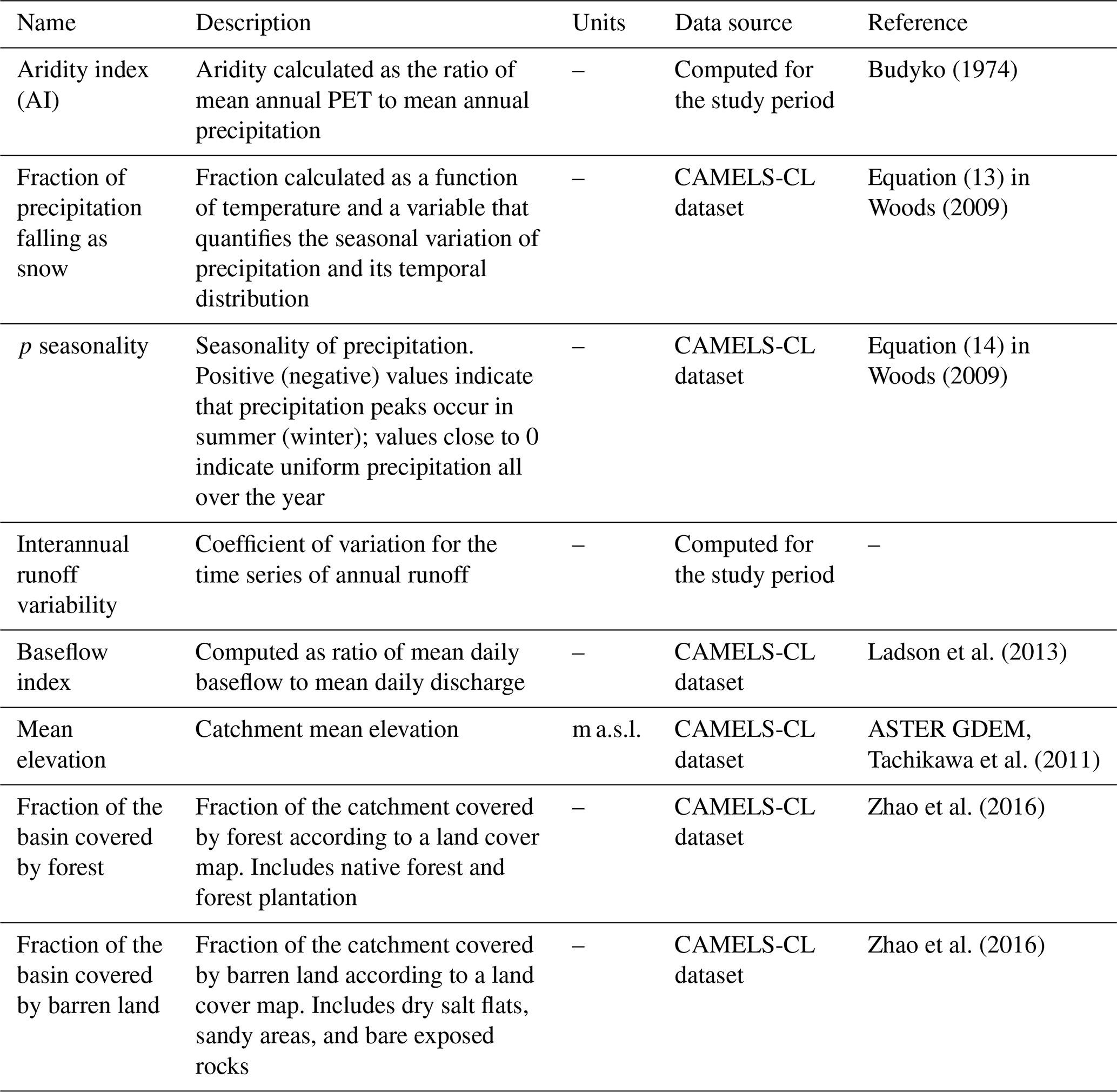
To explore possible relationships between the quality of seasonal streamflow hindcasts and catchment characteristics, we compute, for each combination of hydrological model, initialization time, and objective function, the Spearman's rank correlation coefficient between hindcast performance measures – namely, the CRPSS, the α reliability index, and the coefficient of determination R2 – and selected physiographic–hydroclimatic descriptors (Fig. 3d). To this end, we use the five calibration metrics from Sect. 3.3 and the basin descriptors in Table 4.
Table 4Selected physiographic and climatic characteristics to explore drivers of seasonal forecast quality. Hydroclimatic attributes are computed for the period April 1987–March 2020.
4.1 Example: hydrologic model calibration and ESP results at the upper Maipo River basin
Figure 4 shows observed and simulated daily hydrographs and runoff seasonality for the Maipo at El Manzano River basin (4839 km2), which provides nearly 70 % of municipal water supply for Santiago (Chile's capital city) and is also the primary source of water for agriculture, hydropower, and industry in the area (Ayala et al., 2020). These results were obtained with three calibration objective functions and the three hydrological models. Although these calibration metrics yield skillful seasonal hindcasts for the Maipo at El Manzano River basin (Fig. 5), the simulated hydrographs can be very different, particularly during the target period (September–March). Specifically, the objective function VE-Sep (Fig. 4a3) yields parameter values that cannot properly reproduce daily runoff dynamics (with KGE ranging between −0.27 and 0.40), while the other objective functions provide a more realistic runoff representation (e.g., KGE = 0.68 for the TUW model). Similar results are obtained for runoff seasonality during the evaluation period (Fig. 4b1–b3) and for the remaining basins (see performance metrics for all basins in Fig. S1 of the Supplement).
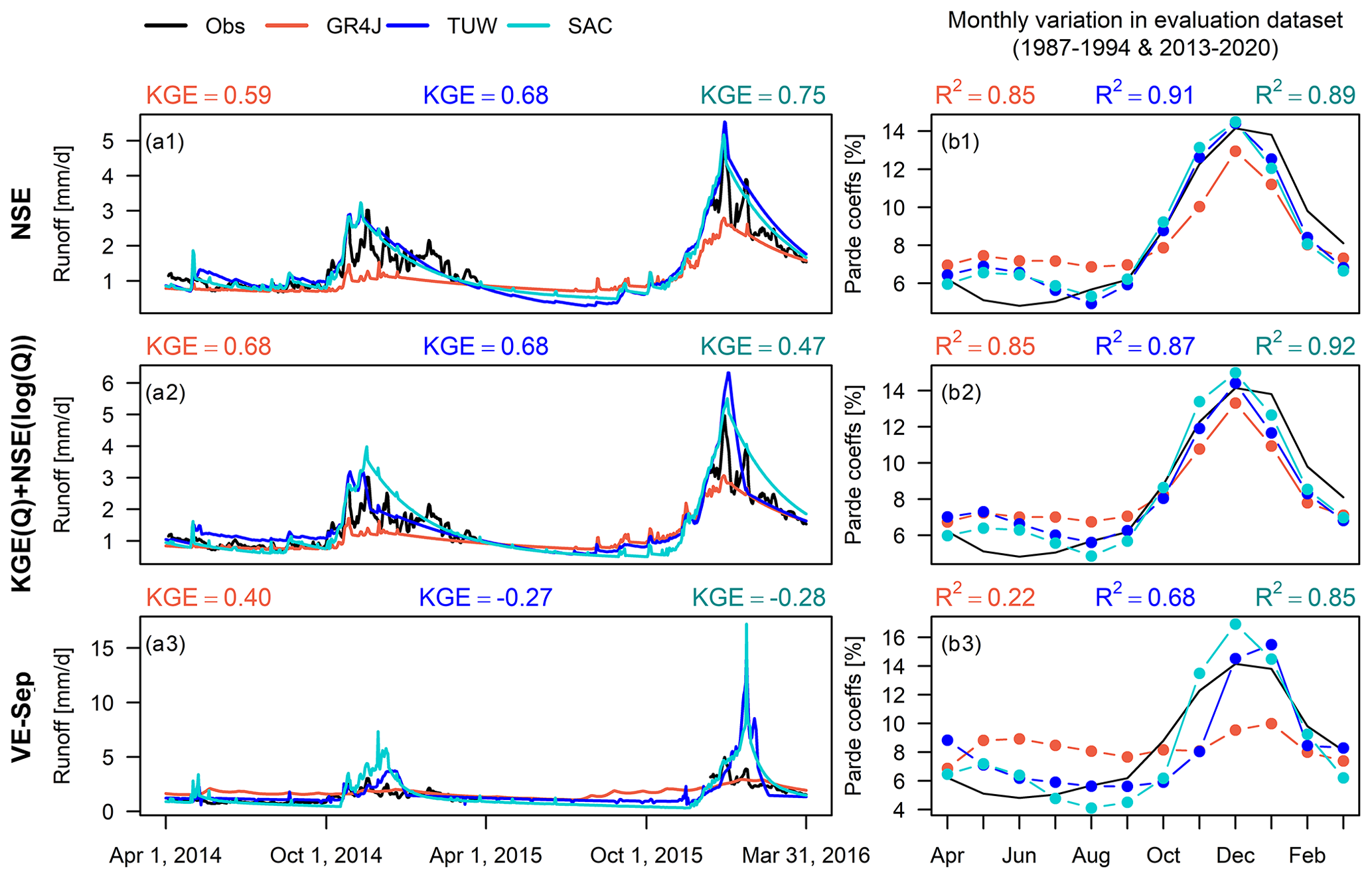
Figure 4(a1–a3) Daily hydrographs (April 2014–March 2016) and (b1–b3) monthly variation curves for the evaluation dataset (April 1987–March 1994 and April 2013–March 2020) at the Maipo at El Manzano River basin, obtained with the three models using parameters obtained from calibrations conducted with NSE, KGE(Q) + NSE(log (Q)) and VE-Sep. The daily KGE obtained with each model is displayed in the left panels, while right panels include the coefficient of determination (R2) between mean monthly simulated and observed runoff averages.
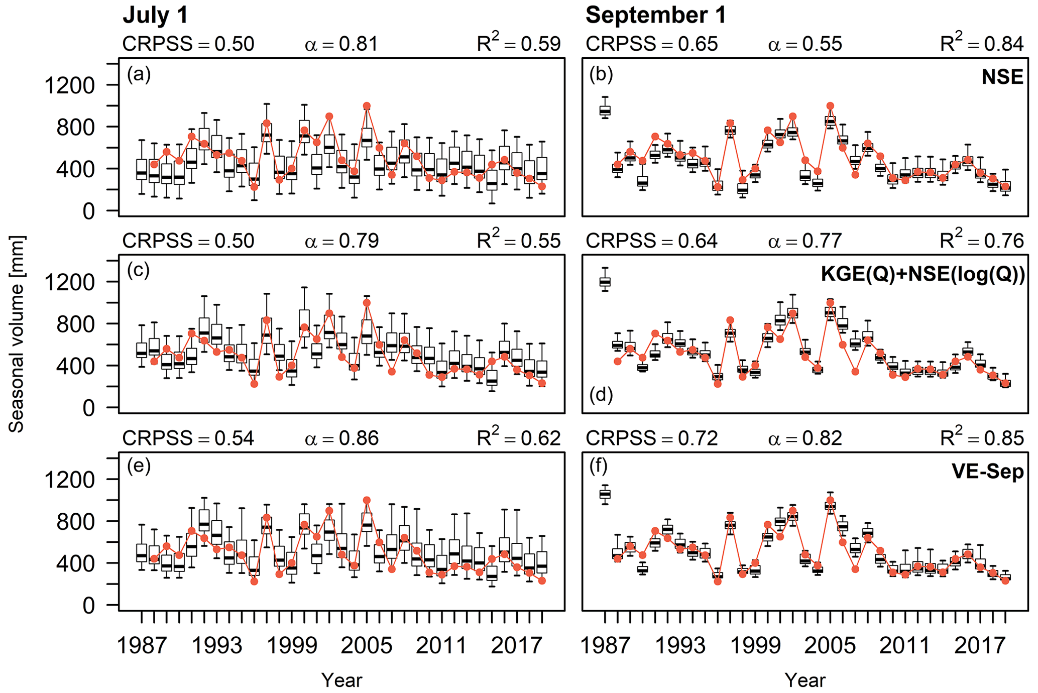
Figure 5Time series with ESP seasonal hindcasts (i.e., September–March runoff) initialized on 1 July (a, c, e), and 1 September (b, d, f) for the Maipo at El Manzano basin. The boxes correspond to the interquartile range (IQR; i.e., 25th and 75th percentiles), the horizontal line in each box is the median, whiskers extend to the of the ensemble, and the red dots represent the observations. The results were produced with the TUW model, using parameters obtained from calibrations conducted with NSE, KGE(Q) + NSE(log (Q)) and VE-Sep (see details in Sect. 3.1). Each panel displays the CRPSS, the reliability index α, and the coefficient of determination R2 (computed using the ensemble hindcast median).
Figure 5 shows sample results of seasonal (i.e., September–March) streamflow hindcasts initialized on 1 July and 1 September for the period April 1987–March 2020 at the Maipo at El Manzano basin, using parameter sets obtained with the same objective functions as in Fig. 4 and the TUW model. As expected, the hindcast initialization time greatly impacts the CRPSS and R2 indices regardless of calibration metric, with substantial improvements towards the beginning of the snowmelt season; conversely, the α reliability index decreases as we approach 1 September (the hindcast ensemble becomes narrower). The results also show that, for those initialization times where IHCs (in particular, snow accumulation at this domain) play a key role in streamflow predictability, the choice of calibration criteria may have large effects on verification metrics (e.g., see α index for 1 September), in contrast to hindcasts initialized on 1 July or earlier dates (see Fig. S2). Further, VE-Sep yields the best performance measures for 1 July and 1 September hindcasts.
4.2 Effects of calibration metric selection on hindcast performance
Figure 6 shows hindcast CRPSS results for our sample of catchments and all initialization times, using the three hydrological models and parameter values obtained with 12 calibration objective functions. In general, the seasonal objective functions (cyan box plots) provide the highest median values across basins for 57 out of 75 combinations (three models × five performance metrics × five initialization times). The highest median performance metric with the TUW model is mainly obtained through seasonal objective functions (11 out of 25 cases, with VE-Sep standing out) and KGE-based metrics (11 out of 25 cases, with ModKGE standing out). When using the GR4J and SAC models, seasonal objective functions dominate, VE-Sep and KGEV-Sep being the best-performing in most cases, respectively. On the other hand, KGE(Q) + KGE() and Split KGE generally yield the poorest hindcast quality across hydrological models. Interestingly, some objective functions enhance the spread in performance metrics across basins – e.g., see CRPSS values obtained with GR4J and SAC; α indices (Fig. S3) and NRMSE (Fig. S4) obtained with SAC using KGE(Q) + KGE() as the calibration metric.
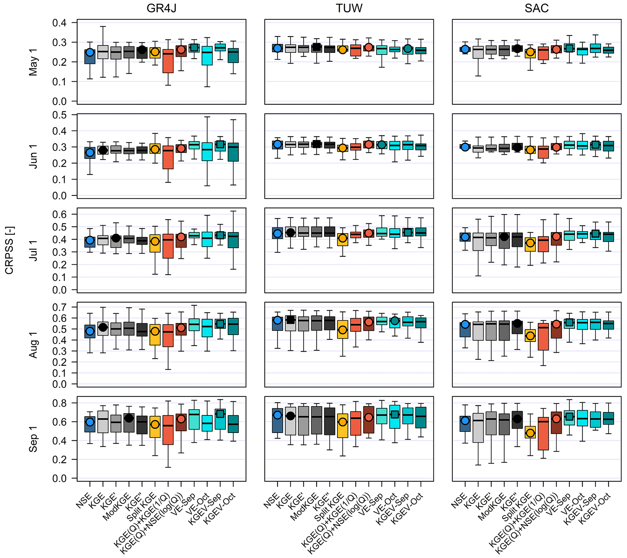
Figure 6Comparison of CRPSS obtained with different calibration objective functions. Each panel contains results for a specific combination of initialization time (rows) and hydrological model (columns), and each box plot comprises results from the 22 case study basins. The boxes correspond to the interquartile range (IQR; i.e., 25th and 75th percentiles), the horizontal line in each box is the median, and whiskers extend to the of the ensemble. The circle indicates the objective function providing the highest median within each family of calibration metric (identified with different colors), and the square indicates the objective function that delivers the best set of metric values using a specific combination of initialization time and hydrological model.
The catchment sample means of all hindcast verification metrics (Table 2) obtained from objective functions belonging to the same family are not significantly different (p values > 0.05 from t tests, not shown), which is valid for the different initialization times considered here. However, there are significant differences between verification means obtained with the best- and the worst-performing calibration metrics. For example, see CRPSS results for 1 September hindcasts obtained from the TUW model (Fig. 5), calibrated with VE-Oct versus Split KGE (p value = 0.03). For hindcasts initialized before 1 July, when the signal from IHCs is weak, the choice of calibration metric becomes less relevant, and the magnitude of differences depends on the forecast verification criteria. For instance, significant differences in percent bias (Fig. S5) are obtained between seasonal and meta-objective seasonal functions, though this is not the case for CRPSS and the α index. Based on these results and additional analyses with the α index, NRMSE, percent bias, and R2 (Figs. S3–S6), we select the overall best-performing (or “representative”) objective function from each family (Table 1) for further analyses, namely NSE, ModKGE, Split KGE, VE-Sep, and KGE(Q) + NSE(log (Q)).
Figure 7 illustrates how initialization time affects hindcast quality attributes when using NSE as the calibration metric and the TUW model. As observed in the upper Maipo River basin (Fig. 5), CRPSS and R2 (the α index) improve (degrades) as hindcasts initializations approach 1 September, with considerable increments in skill on 1 July compared to 1 May and 1 June hindcasts. The skill of 1 May hindcasts is rather low (with CRPSS 5th and 95th percentiles, obtained from the 22 catchments, equal to 0.26 and 0.28, respectively) and does not improve considerably on 1 June. Additionally, inter-basin differences in CRPSS increase as hindcast initializations approach the beginning of the snowmelt season, ranging 0.57–0.69 on 1 September. The same patterns, with small variations in ranges, are observed for the remaining representative objective functions and models (see Figs. S7–S9).
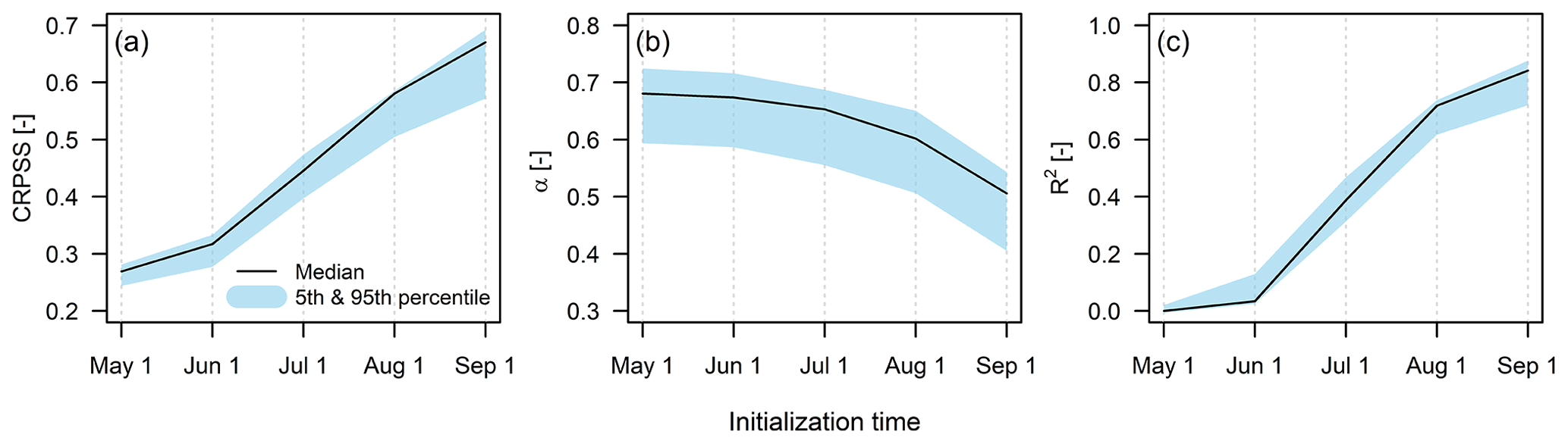
Figure 7Impact of initialization time on (a) CRPSS, (b) the α reliability index, and (c) R2 for seasonal streamflow hindcasts produced with the NSE as calibration objective function and the TUW model. The shades represent the 5th and 95th percentiles in each metric from the 22 case study basins, and the solid line represents the median value from the sample of catchments.
4.3 Seasonal hindcast quality vs. hydrological consistency
We now turn our attention to the following question: to what extent is the quality of seasonal streamflow hindcasts related to the proper simulation of runoff characteristics? Figure 8 displays biases in hydrological signatures for all basins, obtained from the TUW model calibrated with the five selected calibration metrics (the results for GR4J and SAC-SMA are included in Figs. S10 and S11, respectively). Although there is no single best objective function for the signatures examined here, there are some interesting features that are common to all model results:
-
The OFs that yield the largest biases in the mean annual runoff ratio (RR) during the calibration period are Split KGE (median 8.6 %) and VE-Sep (median 12.2 %). However, Split KGE is one of the best OFs in this regard (median bias of 11.8 %) during the evaluation periods, while VE-Sep provides the highest median bias (24.2 %).
-
ModKGE is the OF that provides the lowest biases in high-flow volumes (FHVs) during the calibration period (median bias = 4.7 %), although it is one of the worst OFs (median bias = 38.7 %), along with VE-Sep (median bias = 43.4 %), in the evaluation periods.
-
ModKGE and VE-Sep (KGE(Q) + NSE(log (Q)) and Split KGE) yield the highest (lowest) median biases in low-flow volumes (FLVs) during both calibration and evaluation periods.
-
Split KGE best represents flashiness of runoff (FMS, median bias = 15.0 % during calibration period and 18.2 % in the evaluation periods), while ModKGE (median bias = 26.4 % and 44.2 % during calibration and evaluation periods, respectively) and VE-Sep (median bias = 27.5 % and 33.1 % during calibration and evaluation periods, respectively) are the worst-performing for this signature during both calibration and evaluation periods.
-
Split KGE and KGE(Q) + NSE(log (Q)) (VE-Sep) yield the lowest (highest) biases in median flows (FMM) during both calibration and evaluation periods.
In summary, VE-Sep yields the poorest hydrological consistency across periods and models, and ModKGE provides large biases in streamflow signatures during the evaluation periods. During the calibration period, KGE(Q) + NSE(log (Q)) yields the overall best hydrological consistency, followed by Split KGE and NSE. During the evaluation periods, Split KGE provides, in general, the lowest mean biases in streamflow signatures for all the models, followed by NSE and KGE(Q) + NSE(log (Q)). Interestingly, some objective functions enhance inter-basin differences in signature biases (e.g., compare the spread in RR biases obtained with Split KGE and KGE(Q) + NSE(log (Q)) during the calibration period).
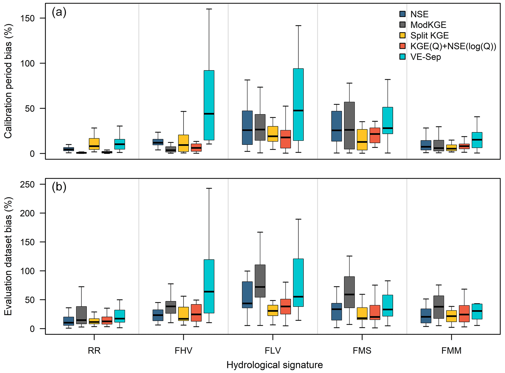
Figure 8Percent biases (y axis) in hydrologic signatures (x axis) obtained with the five representative objective functions and the TUW model for the (a) calibration (April 1994–March 2013) and (b) evaluation dataset (April 1987–March 1994 and April 2013–March 2020). Each box plot comprises results for our 22 case study basins. The boxes correspond to the interquartile range (IQR; i.e., 25th and 75th percentiles), the horizontal line in each box is the median, and whiskers extend to the of the ensemble.
What would be the impacts of selecting a calibration metric yielding good hydrological consistency, instead of a reference objective function that provides the overall best hindcast performance? Figure 9 displays variations in CRPSS (obtained with Eq. 1) using VE-Sep as the reference, for hindcasts initialized on 1 September. It can be noted that Split KGE yields a considerable decrease in hindcast skill compared to the reference (median , and for GR4J, TUW, and SAC, respectively), while ModKGE and KGE(Q) + NSE(log (Q)) yields small ΔCRPSS median values, especially for GR4J and TUW models. Figure 9 also shows that seasonal hindcasts produced with NSE provide generally lower skill than ModKGE and KGE(Q) + NSE(log (Q)); however, NSE yields better hydrological consistency than ModKGE, and worse (similar) biases in signatures than KGE(Q) + NSE(log (Q)) using GR4J and TUW (SAC) models. Overall, the results presented in Fig. 9 show that KGE(Q) + NSE(log (Q)) offers a good compromise between hydrological consistency and hindcast skill.
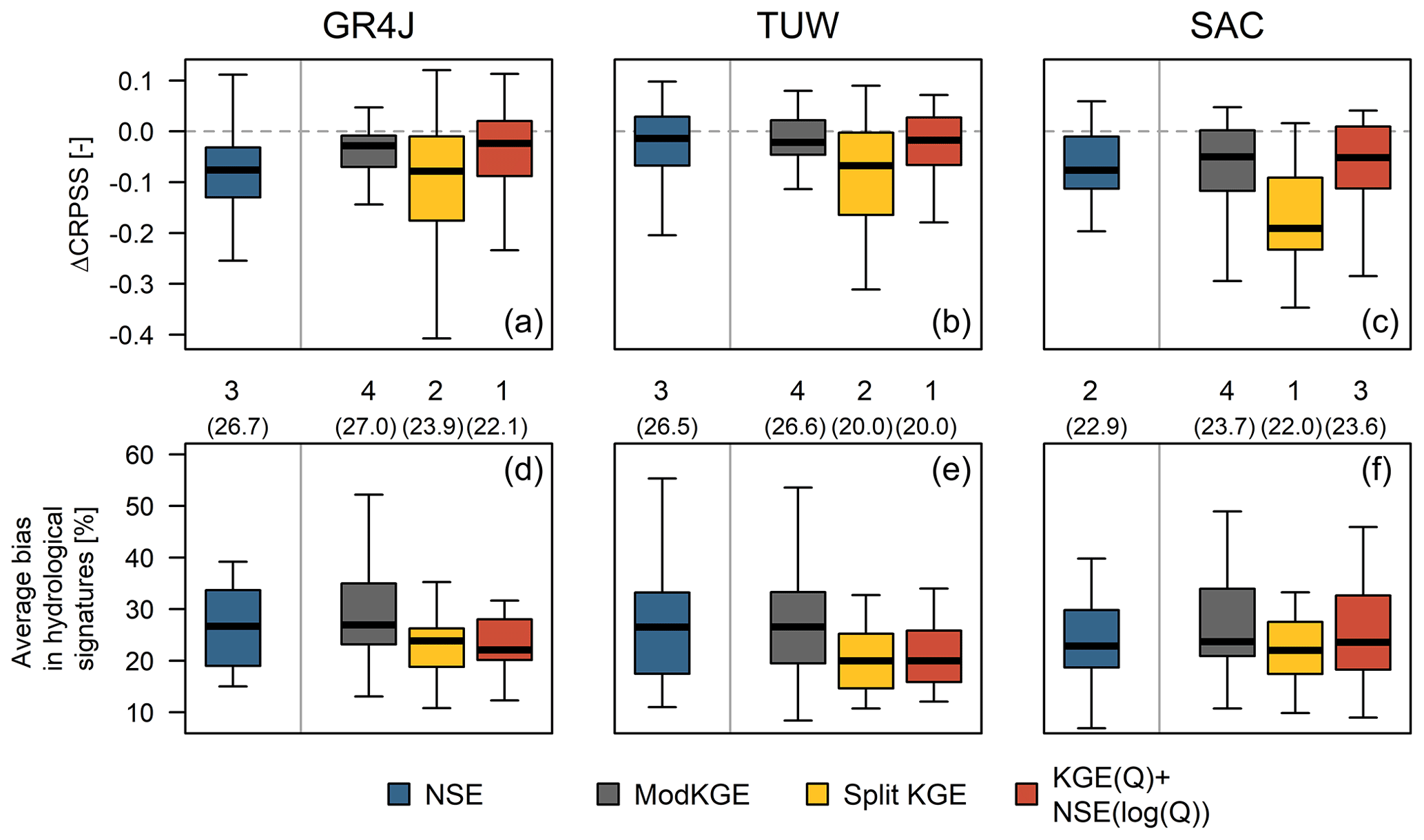
Figure 9Variations in 1 September CRPSS due to the choice of popular and alternative objective functions (shown in different box plots), relative to the best-performing OF in terms of forecast quality (VE-Sep, a–c). The dashed line indicates no difference (i.e., no loss) in forecast performance. (d–f) Average bias in hydrological signatures (computed over the calibration and evaluation periods) with the associated ranking (1 being the best in terms of hydrological consistency) and median average bias obtained from the sample of basins (in parentheses). Each box plot comprises results for our 22 case study basins. The boxes correspond to the interquartile range (IQR; i.e., 25th and 75th percentiles), the horizontal line in each box is the median, and whiskers extend to the of the ensemble.
4.4 Hindcast quality vs. catchment characteristics
We now explore the factors that control seasonal hindcast quality and the extent to which the choice of calibration metric impacts the connections inferred from our sample of catchments. Figure 10 displays results for the TUW model only, and the full results (including GR4J and SAC) are available in the Supplement. In general, the choice of calibration metric affects more the strength, rather than the sign, of the relationships between hindcast quality and catchment attributes. In particular, we find that the correlations between CRPSS and catchment descriptors obtained with Split KGE (which maximizes hydrologic consistency) are weaker than those obtained with other calibration metrics (e.g., see results for baseflow index with the TUW model, interannual runoff variability with all models, and fraction of precipitation falling as snow with all models).
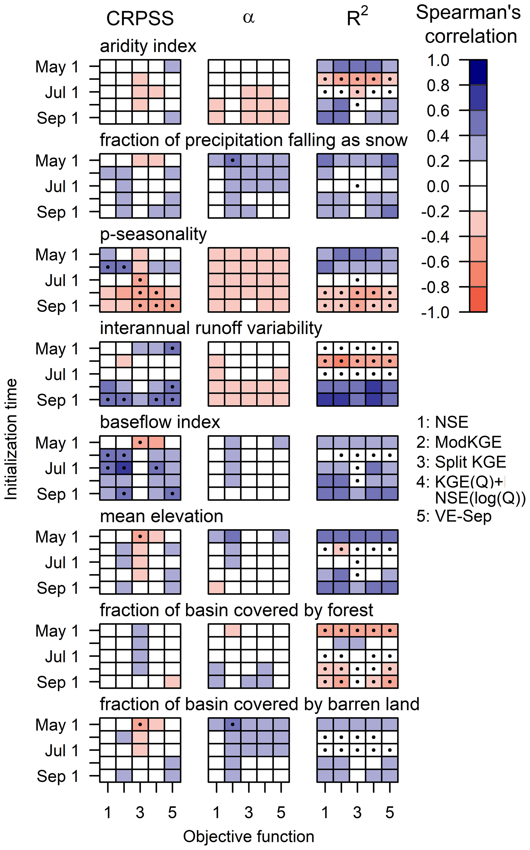
Figure 10Spearman's rank correlation coefficients between catchment characteristics (shown in different rows) and the CRPSS (left), α reliability index (center), and the coefficient of determination R2 (right) obtained for seasonal streamflow hindcasts (period April 1987–March 2020), produced with the five representative objective functions (x axis in each color matrix), different initialization times (y axis in each color matrix), and the TUW model. Black dots indicate statistically significant (p<0.05) correlations.
We find statistically significant correlations between CRPSS and the baseflow index (ρ∼0.2–0.8) with the three models, ModKGE (ρ=0.49), VE-Sep (ρ=0.70), and VE-Sep (ρ=0.41) being the objective functions that maximize such a relationship for 1 September when using TUW (Fig. 10), GR4J, and SAC models (Fig. S12), respectively. Figure 10 shows significant correlations between CRPSS and the interannual variability of runoff (ρ∼0.0–0.6) – especially for 1 September hindcasts (ρ=0.53 for VE-Sep/TUW, ρ=0.64 for ModKGE/GR4J and ρ=0.62 for VE-Sep/SAC). Also positive, but generally weaker, correlations are obtained between hindcast skill and p seasonality ( to 0.0), as well as the fraction of precipitation falling as snow (ρ∼0.0–0.4).
Overall, the α reliability index (Fig. 10, center panels) correlates differently than CRPSS with basin characteristics, with generally smaller values that range between −0.4 and 0.4. Although negative correlations are obtained between interannual runoff variability and α for all models, larger and significant absolute values are only obtained for 1 September hindcasts with the GR4J and SAC models (Fig. S12). The right panels in Fig. 10 show that some catchment descriptors (e.g., baseflow index, interannual variability in runoff) yield similar correlations with R2 compared to those obtained with CRPSS.
5.1 Compromise between hydrological consistency and hindcast performance
The experiments presented here provide insights into the impacts that calibration metric selection may have on the performance of dynamical seasonal forecasting systems in snow-influenced environments, in particular for the traditional ESP technique. Despite the choice of calibration metric being a relevant topic in the hydrologic modeling literature, given the implications for a myriad of water resources applications (see, for example, Shafii and Tolson, 2015; Pool et al., 2017; Melsen et al., 2019; Mizukami et al., 2019), it has received relatively limited attention for the specific case of ensemble seasonal forecasting. Additionally, our sample of catchments offers an interesting experimental setup, spanning an ample range of mountain hydroclimates and physiographic characteristics.
The results presented here reveal tradeoffs between hindcasting skill and hydrological consistency in model simulations. Despite seasonal OFs have produced the best hindcast performance regardless of the hydrological model, they did not result in acceptable hydrological consistency, which was better achieved with time-based meta-objective functions (Split-KGE) or through meta-objective functions with transforms (KGE(Q) + NSE(log (Q))). Conversely, these objective functions resulted in worse hindcast performance than the reference (VE-Sep) calibration metric (e.g., a 10 %, 10 % and 26 % loss in CRPSS for 1 September using Split KGE with GR4J, TUW and SAC-SMA models, respectively). These results highlight the risk of selecting model configurations for a specific purpose without complementary insights into the representation of features that may be useful for other operational applications. Among the options examined here, KGE(Q) + NSE(log (Q)) provided the best compromise between hydrological consistency and hindcast skill, with only a median 5 % loss in CRPSS for 1 September hindcasts.
5.2 Initialization times and hindcast skill
ESP hindcasts produced at the beginning of the snowmelt season for our set of catchments are very skillful (median CRPSS ∼ 0.62–0.67 for seasonal OFs, CRPSS ∼ 0.60–0.64 for meta-objective OFs with transformations, and 0.60–0.62 for KGE-type OF), and the skill decreased monotonically with longer lead times, regardless of the choice of calibration OF and model. Importantly, hindcast skill improves considerably between 1 June and 1 July, reflecting that the information on snow accumulation collected at the end of fall and beginning of the winter season is crucial to maximize the predictability from IHCs in Andean catchments. These results align well with previous studies in other snow-influenced mountain environments and cold regions of the world, such as the Colorado River basin (Franz et al., 2003; Baker et al., 2021), the US Pacific Northwest (Mendoza et al., 2017), and northern Europe (Pechlivanidis et al., 2020; Girons Lopez et al., 2021). More generally, this study reinforces – through multiple hydrologic model setups – the decay of ESP hindcast skill with lead time, which has also been reported in domains where snow has a limited influence on the water cycle (e.g., Harrigan et al., 2018; Donegan et al., 2021).
5.3 Factors controlling seasonal forecast quality
Our results reaffirm that seasonal forecast quality is better in slow-reacting basins with a higher baseflow contribution (Harrigan et al., 2018; Pechlivanidis et al., 2020; Donegan et al., 2021; Girons Lopez et al., 2021) and with a higher amount of precipitation falling as snow, in agreement with previous studies conducted over large domains (e.g., Arnal et al., 2018; Wanders et al., 2019). In our study area, seasonal hindcast quality is also explained by high interannual runoff variability – with significant correlations on 1 September and 1 August – which is a characteristic feature of snow-dominated headwater catchments in central Chile (i.e., between 27 and 37∘ S), where year-to-year variability in mean annual precipitation is also considerable (Hernandez et al., 2022). In the driest (northernmost) catchments, only a few sporadic storms contribute to annual precipitation amounts (Hernandez et al., 2022), and the high skewness of daily runoff challenges the calibration of hydrological models. On the other hand, the predictability from future meteorological forcings is becoming important in the wetter southern hydroclimates since occasional spring precipitation events may have a strong effect on total spring–summer runoff volumes.
5.4 Inter-model differences
In this study, we obtained similar effects of calibration criteria selection across model structures, though the latter provide differences in hindcast performance and hydrological consistency. Despite the three models being in the lower zone of the spatial resolution–process complexity continuum (Hrachowitz and Clark, 2017), they greatly differ in the number of parameters, and such differences do not necessarily relate to seasonal forecast quality. In fact, the TUW model (15 parameters) provides generally better ESP hindcasts than GR4J (6 parameters) and SAC-SMA (28 parameters). In addition to discrepancies related to soil storages and associated parameterizations, the models differ in terms of their snow modules – which is a key component for seasonal predictability in mountainous basins – with 2, 5, and 10 free parameters within GR4J, TUW, and SAC-SMA models, respectively. The snow routines used in GR4J (CemaNeige; Valéry et al., 2014b) and TUW (Parajka et al., 2007) models follow a simple degree-day factor approach, differing mainly in the characterization of precipitation phase (the TUW model allows for a mix of rain and snow) and the melt temperature threshold (set as 0 ∘C for the GR4J model and defined as a free-parameter in the TUW model). On the other hand, Snow-17 (snow routine coupled to SAC-SMA) is based on a simplified energy balance (Anderson, 1973). Both CemaNeige and Snow-17 models estimate precipitation phase using a single temperature threshold (i.e., precipitation can occur only as rain or snow). Finally, both the TUW snow routine and the Snow-17 model include a parameter to correct snowfall undercatch.
The results presented here, the inter-model differences described above, and previous work on the implications of precipitation phase partitioning (Harder and Pomeroy, 2014; e.g., Valéry et al., 2014a; Harpold et al., 2017) suggest that a gradual transition between rain and snow (as in the TUW model) may favor seasonal streamflow forecast performance in snow-influenced regimes, especially in catchments with large elevation ranges and extended snowmelt seasons (Girons Lopez et al., 2020). However, testing such hypothesis is out of the scope of this study, for which controlled modeling experiments would be required.
5.5 Impacts of verification sample size
When the hindcasted year overlaps with the calibration period (as it happens with our experimental setup), the hydrological model gains information from meteorological inputs, even if the climate time series observed during that year are excluded from the generation of ESP hindcasts. In spite of this, we decided to take advantage of the entire 33-year period for hindcast verification, since small sample sizes (i.e., number of WYs) have been widely recognized as a serious limitation within the seasonal forecasting literature (e.g., Shi et al., 2015; Trambauer et al., 2015; Mendoza et al., 2017; Lucatero et al., 2018; Wood et al., 2018). This strategy enables a more robust assessment of seasonal hindcast quality, as opposed to using only the 14 WYs left for model evaluation. To demonstrate this point, we characterized the impact of sample size on the spread of CRPSS results by performing a bootstrap analysis with 1000 realizations for the Maipo River basin, using hindcasts produced with the TUW model and KGE(Q) + NSE(log (Q)) as the calibration metric (Fig. 11). The analysis was conducted for the following verification samples: (a) a full period (i.e., 33 WYs), using the parameter set obtained by calibrating the model with data from the period April 1994–March 2013; (b) a full period, using parameter sets re-calibrated with all data except the hindcasted year (i.e., 33 parameter sets to produce 33 seasonal hindcasts); (c) a calibration period (i.e., 19 WYs), using a single parameter set obtained with data from the same period; (d) evaluation dataset periods (i.e., 14 WYs between April 1987–March 1994 and April 2013–March 2020), using the same parameter set as in case (c); and (e) a dry hydroclimatic period (14 WYs between April 2006–March 2020), using the same parameter set as in case (c).
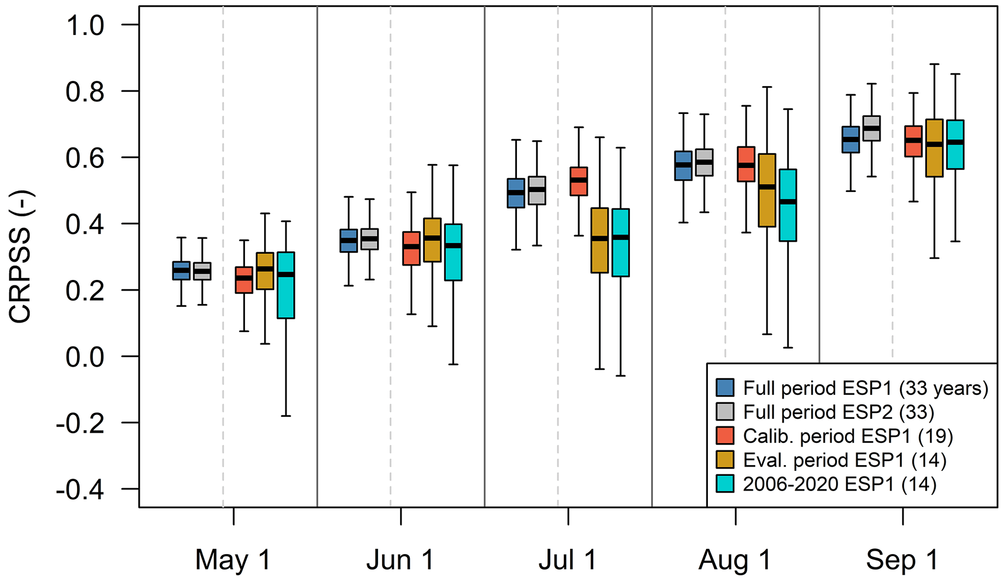
Figure 11Comparison of CRPSS values for seasonal (i.e., September–March) streamflow hindcasts produced at the Maipo River basin with the TUW model and KGE(Q) + NSE(log (Q)) as the calibration metric. Each box comprises results from 1000 bootstraps with replacement applied to different verification sample sizes (i.e., number of hindcast–observation pairs): (a) a full period (i.e., 33 WYs), using the same parameter set, obtained by calibrating the model with data from the period April 1994–March 2013 (blue); (b) a full period, using parameter sets re-calibrated with all data except the hindcasted year (i.e., 33 parameter sets to produce 33 seasonal hindcasts, gray); (c) 19 WYs (calibration period), using a single parameter set obtained with data from the same period (red); (d) 14 WYs (i.e., evaluation data set April 1987–March 1994 and April 2013–March 2020), using the same parameter set as in case (c) (orange); and (e) 14 WYs (April 2006–March 2020), using the same parameter set as in case (c) (cyan). The boxes correspond to the interquartile range (IQR; i.e., 25th and 75th percentiles), the horizontal line in each box is the median, and the whiskers extend to the of the ensemble.
The results in Fig. 11 show a considerable spread in CRPSS arising from sampling uncertainty when using 14-year verification periods (orange and cyan boxes). Additionally, the median CRPSS results are lower than those obtained with 19 and 33 WYs in 1 July, 1 August and 1 September. An interesting result is the similarity of CRPSS values obtained with scenarios (a) and (b), suggesting that the hindcasting generation and verification approach adopted here (i.e., using a single parameter set obtained by calibrating will all the years with available observations) is a good proxy to characterize the hindcast quality that would be obtained with an operational setup that considers parameter re-calibration for each forecasted season.
Finally, we examined the sensitivity of the CRPSS for 1 September hindcasts to the stratification of the full verification sample (i.e., 33 WYs) between hydrologic model calibration (April 1994–March 2013; i.e., 19 WYs) and evaluation (April 1987–March 1994 and April 2013–March 2020; i.e., 14 WYs) datasets (Fig. 12). Here, we used parameters calibrated with the five representative OFs and the TUW model, using data from the period April 1994–March 2013. The results show that the VE-Sep remains the top-performing objective function in terms of CRPSS, while Split KGE yields the worst results. Further, the rankings of the other objective functions (NSE, ModKGE, and KGE(Q) + NSE(log (Q))) vary depending on the verification period, and CRPSS values are higher during the calibration period compared to the evaluation dataset.
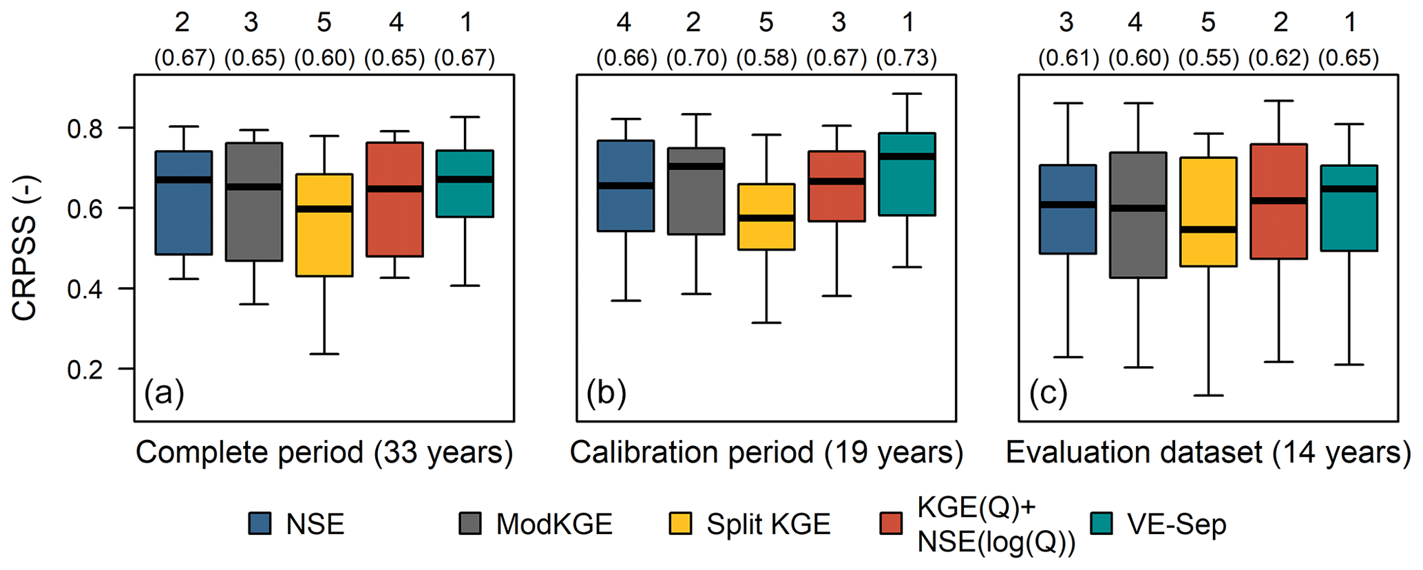
Figure 12Comparison of CRPSS for 1 September hindcasts obtained with the five representative objective functions and the TUW model. Each panel contains results for a different hindcast verification period: (a) 33 WYs (full period), (b) 19 WYs (calibration period), and (c) 14 WYs (i.e., evaluation data set April 1987–March 1994 and April 2013–March 2020). Each box plot comprises results from the 22 case study basins and one objective function. The boxes correspond to the interquartile range (IQR; i.e., 25th and 75th percentiles), the horizontal line in each box is the median, and whiskers extend to the of the ensemble. The numbers in parentheses denote the median CRPSS among all basins and the numbers above the OF ranking based on that median, 1 being the best.
5.6 Limitations and future work
In this study, we used a global, single-objective optimization algorithm to find the “best” parameter set given a combination of forcing, model structure, and calibration objective function; hence, we did not explore the potential effects of parameter equifinality, since such analysis is out of the scope of this work. Recently, Muñoz-Castro et al. (2023) examined the effects of calibration metric selection and parameter equifinality on the level of (dis)agreement in parameter values across 95 catchments in Chile, finding that (i) the choice of objective function has smaller effects on parameter values in catchments with a low aridity index and high mean annual runoff ratio, in contrast to drier climates, and (ii) catchments with better parameter agreement also provide better performance across model structures and simulation periods. Future work could explore whether such performance in streamflow simulations translates well into seasonal forecast quality attributes. Additionally, calibration strategies (e.g., Gharari et al., 2013; Fowler et al., 2018b) and model selection frameworks (e.g., Saavedra et al., 2022) advocating for consistent performance across different hydroclimatic conditions could be explored for seasonal forecasting applications.
Our assessment of hydrological consistency is solely based on the model's ability to reproduce streamflow characteristics, though snow depth (Tuo et al., 2018; Sleziak et al., 2020), snow water equivalent (e.g., Nemri and Kinnard, 2020), or snow-covered area (e.g., Şorman et al., 2009; Duethmann et al., 2014), or the combination of these and other in situ or remotely sensed variables (e.g., Kunnath-Poovakka et al., 2016; Nijzink et al., 2018; Tong et al., 2021) could be incorporated to achieve a more exhaustive evaluation of model realism. Moreover, multivariate calibration methods using multi-objective optimization algorithms (e.g., Yapo et al., 1998; Pokhrel et al., 2012; Shafii and Tolson, 2015) may be considered to examine potential improvements in hydrological consistency and streamflow forecast quality compared to traditional parameter estimation approaches.
The data, models, and results obtained here provide a test bed for the systematic implementation of new tools aimed at improving seasonal streamflow forecasts in snow-dominated Andean catchments. Ongoing work is focused on developing a historical ensemble gridded meteorological product for our study area, the implementation of data assimilation methods for improved estimates of initial conditions, the assessment of seasonal climate forecast products, and the inclusion of additional catchments. Given the strong relationships between basin-scale hydrology in this domain and some large-scale climate patterns (e.g., El Niño–Southern Oscillation; Hernandez et al., 2022), future research should explore the potential of post-processing techniques that take advantage of climate information to improve forecast quality (e.g., Hamlet and Lettenmaier, 1999; Werner et al., 2004; Yuan and Zhu, 2018; Donegan et al., 2021). Finally, the hindcast generation and verification analyses presented here should be extended to fall and winter seasons, which are relevant for domestic water supply and other applications.
Dynamical systems have been implemented by many organizations across the globe for operational seasonal streamflow forecasting. Despite their reliance on hydrological models, no detailed assessments have been conducted to understand how the choice of calibration metric affects the quality attributes of seasonal streamflow forecasts, their connection with simulated streamflow characteristics, and the relationship between forecast quality and catchment descriptors. Here, we provide important insights using the traditional ensemble streamflow prediction (ESP) method to generate seasonal hindcasts of spring/summer streamflow in 22 basins in central Chile, where snow plays a key role in the hydrologic cycle. We use three popular conceptual rainfall-runoff models calibrated with 12 metrics from different families of objective functions. The main conclusions are as follows:
-
The choice of calibration metric yields considerable differences in hindcast quality (except R2) for winter initialization times. Such an effect decreases considerably for hindcasts initialized during the fall season.
-
The comparison of seasonal hindcasts obtained from different families of objective functions revealed that hydrological consistency does not ensure satisfactory seasonal ESP forecasts (e.g., Split KGE) and that satisfactory ESP forecasts are not necessarily associated with hydrologically consistent streamflow simulations (e.g., VE-Sep).
-
We could identify at least one objective function (KGE(Q) + NSE(log (Q))) that yields a reasonable balance between hydrological consistency and hindcast performance.
-
The baseflow index and the interannual runoff variability are the strongest predictors of probabilistic skill and R2 across objective functions and models. Moreover, the choice of calibration metric generally affects the strength of the relationship between forecast quality and catchment attributes.
The results presented here highlight the importance of hydrologic model calibration in producing skillful seasonal streamflow forecasts and drawing robust conclusions on hydrological predictability. Improving parameter estimation strategies can benefit not only operational systems relying on dynamical methods but also a myriad of hybrid approaches designed to leverage information from hydrologic model outputs. By advancing our understanding of the complex interplay between calibration metrics, model performance, and catchment characteristics, our study contributes to the ongoing effort to enhance the accuracy and reliability of streamflow forecasts in snow-influenced domains, to support informed water resources management decisions.
All the data and models used to produce the results included in this paper here are publicly available at Zenodo (Araya et al., 2023; https://doi.org/10.5281/zenodo.7853556).
The supplement related to this article is available online at: https://doi.org/10.5194/hess-27-4385-2023-supplement.
DA, PM, and EMC conceptualized the study and designed the overall approach. DA conducted all the model simulations, generated the hindcasts, analyzed the results, and created all the figures. PM and EMC provided support to set up the scripts used in this study. All the authors contributed to the refinement of the methodology and analysis framework; discussed the results; and contributed to the writing, reviewing, and editing of the manuscript.
The contact author has declared that none of the authors has any competing interests.
Publisher's note: Copernicus Publications remains neutral with regard to jurisdictional claims made in the text, published maps, institutional affiliations, or any other geographical representation in this paper. While Copernicus Publications makes every effort to include appropriate place names, the final responsibility lies with the authors.
The authors thank the editor (Rohini Kumar), Paul C. Astagneau, and two anonymous reviewers, whose detailed and thoughtful comments greatly improved the manuscript.
Pablo A. Mendoza received support from FONDECYT, project no. 11200142. Pablo A. Mendoza and James McPhee received support from CONICYT/PIA, project no. AFB230001.
This paper was edited by Rohini Kumar and reviewed by Paul C. Astagneau and two anonymous referees.
Addor, N. and Melsen, L. A.: Legacy, Rather Than Adequacy, Drives the Selection of Hydrological Models, Water Resour. Res., 55, 378–390, https://doi.org/10.1029/2018WR022958, 2019.
Alvarez-Garreton, C., Mendoza, P. A., Pablo Boisier, J., Addor, N., Galleguillos, M., Zambrano-Bigiarini, M., Lara, A., Puelma, C., Cortes, G., Garreaud, R., McPhee, J., and Ayala, A.: The CAMELS-CL dataset: Catchment attributes and meteorology for large sample studies-Chile dataset, Hydrol. Earth Syst. Sci., 22, 5817–5846, https://doi.org/10.5194/hess-22-5817-2018, 2018.
Anderson, E.: National Weather Service River Forecast system – snow accumulation and ablation model, NOAA Tech. Memo. NWS HYDRO-17, NOAA, https://repository.library.noaa.gov/view/noaa/13507 (last access: 23 March 2023), 1973.
Araya, D., Mendoza, P. A., McPhee, J., and Muñoz-Castro, E.: A hydrological modeling dataset for ensemble streamflow forecasting in 22 snow-influenced basins in Central Chile, Zenodo [code and data set], https://doi.org/10.5281/zenodo.7853556, 2023.
Arnal, L., Cloke, H. L., Stephens, E., Wetterhall, F., Prudhomme, C., Neumann, J., Krzeminski, B., and Pappenberger, F.: Skilful seasonal forecasts of streamflow over Europe?, Hydrol. Earth Syst. Sci., 22, 2057–2072, https://doi.org/10.5194/hess-22-2057-2018, 2018.
Ayala, Á., Farías-Barahona, D., Huss, M., Pellicciotti, F., McPhee, J., and Farinotti, D.: Glacier runoff variations since 1955 in the Maipo River basin, in the semiarid Andes of central Chile, The Cryosphere, 14, 2005–2027, https://doi.org/10.5194/tc-14-2005-2020, 2020.
Baez-Villanueva, O. M., Zambrano-Bigiarini, M., Mendoza, P. A., McNamara, I., Beck, H. E., Thurner, J., Nauditt, A., Ribbe, L., and Thinh, N. X.: On the selection of precipitation products for the regionalisation of hydrological model parameters, Hydrol. Earth Syst. Sci., 25, 5805–5837, https://doi.org/10.5194/hess-25-5805-2021, 2021.
Baker, S. A., Rajagopalan, B., and Wood, A. W.: Enhancing Ensemble Seasonal Streamflow Forecasts in the Upper Colorado River Basin Using Multi-Model Climate Forecasts, J. Am. Water Resour. Assoc., 57, 906–922, https://doi.org/10.1111/1752-1688.12960, 2021.
Bergström, S.: Development and application of a conceptual runoff model for Scandinavian catchments, Report RHO 7, SMHI, Norrköping, Sweden, http://www.diva-portal.org/smash/record.jsf?pid=diva2:1456191&dswid=-4221 (last access: 8 March 2023), 1976.
Bohn, T. J., Sonessa, M. Y., and Lettenmaier, D. P.: Seasonal hydrologic forecasting: Do multimodel ensemble averages always yield improvements in forecast skill?, J. Hydrometeorol., 11, 1358–1372, https://doi.org/10.1175/2010JHM1267.1, 2010.
Boisier, J. P., Alvarez-Garretón, C., Cepeda, J., Osses, A., Vásquez, N., and Rondanelli, R.: CR2MET: A high-resolution precipitation and temperature dataset for hydroclimatic research in Chile, Center for Climate and Resilience Research [data set], https://www.cr2.cl/datos-productos-grillados/ (last access: 11 March 2023), 2018.
Budyko, M. I.: Climate and Life, Academic Press, London, ISBN 9780080954530, 1974.
Burnash, R., Ferral, R., and McGuire, R.: A generalized streamflow simulation system – Conceptual modeling for digital computers, Sacramento, California, https://searchworks.stanford.edu/view/753303 (last access: 7 March 2023), 1973.
Cook, B. I., Smerdon, J. E., Cook, E. R., Williams, A. P., Anchukaitis, K. J., Mankin, J. S., Allen, K., Andreu-Hayles, L., Ault, T. R., Belmecheri, S., Coats, S., Coulthard, B., Fosu, B., Grierson, P., Griffin, D., Herrera, D. A., Ionita, M., Lehner, F., Leland, C., Marvel, K., Morales, M. S., Mishra, V., Ngoma, J., Nguyen, H. T. T., O'Donnell, A., Palmer, J., Rao, M. P., Rodriguez-Caton, M., Seager, R., Stahle, D. W., Stevenson, S., Thapa, U. K., Varuolo-Clarke, A. M., and Wise, E. K.: Megadroughts in the Common Era and the Anthropocene, Nat. Rev. Earth Environ., 3, 741–757, https://doi.org/10.1038/s43017-022-00329-1, 2022.
Cornwell, E., Molotch, N. P., and McPhee, J.: Spatio-temporal variability of snow water equivalent in the extra-tropical Andes Cordillera from distributed energy balance modeling and remotely sensed snow cover, Hydrol. Earth Syst. Sci., 20, 411–430, https://doi.org/10.5194/hess-20-411-2016, 2016.
Coron, L., Thirel, G., Delaigue, O., Perrin, C., and Andréassian, V.: The suite of lumped GR hydrological models in an R package, Environ. Model. Softw., 94, 166–171, https://doi.org/10.1016/j.envsoft.2017.05.002, 2017.
Crochemore, L., Ramos, M.-H., and Pappenberger, F.: Bias correcting precipitation forecasts to improve the skill of seasonal streamflow forecasts, Hydrol. Earth Syst. Sci., 20, 3601–3618, https://doi.org/10.5194/hess-20-3601-2016, 2016.
Crochemore, L., Ramos, M. H., Pappenberger, F., and Perrin, C.: Seasonal streamflow forecasting by conditioning climatology with precipitation indices, Hydrol. Earth Syst. Sci., 21, 1573–1591, https://doi.org/10.5194/hess-21-1573-2017, 2017.
Crochemore, L., Ramos, M. H., and Pechlivanidis, I. G.: Can Continental Models Convey Useful Seasonal Hydrologic Information at the Catchment Scale?, Water Resour. Res., 56, 1–21, https://doi.org/10.1029/2019WR025700, 2020.
Day, G. N.: Extended Streamflow Forecasting Using NWSRFS, J. Water Resour. Pl. Manage., 111, 157–170, https://doi.org/10.1061/(ASCE)0733-9496(1985)111:2(157), 1985.
DeChant, C. M. and Moradkhani, H.: Toward a reliable prediction of seasonal forecast uncertainty: Addressing model and initial condition uncertainty with ensemble data assimilation and Sequential Bayesian Combination, J. Hydrol., 519, 2967–2977, https://doi.org/10.1016/j.jhydrol.2014.05.045, 2014.
DGA: Actualización del balance hídrico nacional, SIT No. 417, Ministerio de Obras Públicas, Dirección General de Aguas, División de Estudios y Planificación, Santiago, Chile, https://snia.mop.gob.cl/repositoriodga/handle/20.500.13000/6961 (last access: 24 March 2023), 2017.
DGA: Pronóstico de caudales de deshielo periodo septiembre/2022-marzo/2023, SDT No. 448, https://snia.mop.gob.cl/repositoriodga/handle/20.500.13000/125978 (last access: 22 March 2023), 2022.
Donegan, S., Murphy, C., Harrigan, S., Broderick, C., Foran Quinn, D., Golian, S., Knight, J., Matthews, T., Prudhomme, C., Scaife, A. A., Stringer, N., and Wilby, R. L.: Conditioning ensemble streamflow prediction with the North Atlantic Oscillation improves skill at longer lead times, Hydrol. Earth Syst. Sci., 25, 4159–4183, https://doi.org/10.5194/hess-25-4159-2021, 2021.
Duan, Q., Sorooshian, S., and Gupta, V.: Effective and Efficient Global Optimization for Conceptual Rainfal-Runoff Models, Water Resour. Res., 28, 1015–1031, 1992.
Duethmann, D., Peters, J., Blume, T., Vorogushyn, S., and Güntner, A.: The value of satellite-derived snow cover images for calibrating a hydrological model in snow-dominated catchments in Central Asia, Water Resour. Res., 50, 2002–2021, https://doi.org/10.1002/2013WR014382, 2014.
Fowler, K., Peel, M., Western, A., and Zhang, L.: Improved Rainfall-Runoff Calibration for Drying Climate: Choice of Objective Function, Water Resour. Res., 54, 3392–3408, https://doi.org/10.1029/2017WR022466, 2018a.
Fowler, K., Coxon, G., Freer, J., Peel, M., Wagener, T., Western, A., Woods, R., and Zhang, L.: Simulating Runoff Under Changing Climatic Conditions: A Framework for Model Improvement, Water Resour. Res., 54, 9812–9832, https://doi.org/10.1029/2018WR023989, 2018b.
Franz, K. J., Hartmann, H. C., Sorooshian, S., and Bales, R.: Verification of National Weather Service Ensemble Streamflow Predictions for water supply forecasting in the Colorado River Basin, J. Hydrometeorol., 4, 1105–1118, https://doi.org/10.1175/1525-7541(2003)004<1105:VONWSE>2.0.CO;2, 2003.
Garreaud, R., Alvarez-Garreton, C., Barichivich, J., Pablo Boisier, J., Christie, D., Galleguillos, M., LeQuesne, C., McPhee, J., and Zambrano-Bigiarini, M.: The 2010–2015 megadrought in central Chile: Impacts on regional hydroclimate and vegetation, Hydrol. Earth Syst. Sci., 21, 6307–6327, https://doi.org/10.5194/hess-21-6307-2017, 2017.
Garreaud, R. D., Boisier, J. P. P., Rondanelli, R., Montecinos, A., Sepúlveda, H. H. H., and Veloso-Aguila, D.: The Central Chile Mega Drought (2010–2018): A climate dynamics perspective, Int. J. Climatol., 40, 1–19, https://doi.org/10.1002/joc.6219, 2019.
Gharari, S., Hrachowitz, M., Fenicia, F., and Savenije, H. H. G.: An approach to identify time consistent model parameters: Sub-period calibration, Hydrol. Earth Syst. Sci., 17, 149–161, https://doi.org/10.5194/hess-17-149-2013, 2013.
Girons Lopez, M., Vis, M. J. P., Jenicek, M., Griessinger, N., and Seibert, J.: Assessing the degree of detail of temperature-based snow routines for runoff modelling in mountainous areas in central Europe, Hydrol. Earth Syst. Sci., 24, 4441–4461, https://doi.org/10.5194/hess-24-4441-2020, 2020.
Girons Lopez, M., Crochemore, L., and G. Pechlivanidis, I.: Benchmarking an operational hydrological model for providing seasonal forecasts in Sweden, Hydrol. Earth Syst. Sci., 25, 1189–1209, https://doi.org/10.5194/hess-25-1189-2021, 2021.
Giuliani, M., Crochemore, L., Pechlivanidis, I., and Castelletti, A.: From skill to value: isolating the influence of end user behavior on seasonal forecast assessment, Hydrol. Earth Syst. Sci., 24, 5891–5902, https://doi.org/10.5194/hess-24-5891-2020, 2020.
Greuell, W., Franssen, W. H. P., and Hutjes, R. W. A.: Seasonal streamflow forecasts for Europe – Part 2: Sources of skill, Hydrol. Earth Syst. Sci., 23, 371–391, https://doi.org/10.5194/hess-23-371-2019, 2019.
Gupta, H. V., Kling, H., Yilmaz, K. K., and Martinez, G. F.: Decomposition of the mean squared error and NSE performance criteria: Implications for improving hydrological modelling, J. Hydrol., 377, 80–91, https://doi.org/10.1016/j.jhydrol.2009.08.003, 2009.
Hamlet, A. F. and Lettenmaier, D. P.: Effects of climate change on hydrology and water resources in the Columbia River basin, J. Am. Water Resour. Assoc., 35, 1597–1623, 1999.
Harder, P. and Pomeroy, J. W.: Hydrological model uncertainty due to precipitation-phase partitioning methods, Hydrol. Process., 28, 4311–4327, https://doi.org/10.1002/hyp.10214, 2014.
Hargreaves, G. H. and Samani, Z. A.: Reference Crop Evapotranspiration from Temperature, Appl. Eng. Agric., 1, 96–99, https://doi.org/10.13031/2013.26773, 1985.
Harpold, A. A., Kaplan, M. L., Zion Klos, P., Link, T., McNamara, J. P., Rajagopal, S., Schumer, R., and Steele, C. M.: Rain or snow: Hydrologic processes, observations, prediction, and research needs, Hydrol. Earth Syst. Sci., 21, 1–22, https://doi.org/10.5194/hess-21-1-2017, 2017.
Harrigan, S., Prudhomme, C., Parry, S., Smith, K., and Tanguy, M.: Benchmarking ensemble streamflow prediction skill in the UK, Hydrol. Earth Syst. Sci., 22, 2023–2039, https://doi.org/10.5194/hess-22-2023-2018, 2018.
Hernandez, D., Mendoza, P. A., Boisier, J. P., and Ricchetti, F.: Hydrologic Sensitivities and ENSO Variability Across Hydrological Regimes in Central Chile (28∘–41∘ S), Water Resour. Res., 58, e2021WR031860, https://doi.org/10.1029/2021WR031860, 2022.
Hersbach, H.: Decomposition of the Continuous Ranked Probability Score for Ensemble Prediction Systems, Weather Forecast., 15, 559–570, https://doi.org/10.1175/1520-0434(2000)015<0559:DOTCRP>2.0.CO;2, 2000.
Hrachowitz, M. and Clark, M. P.: HESS Opinions: The complementary merits of competing modelling philosophies in hydrology, Hydrol. Earth Syst. Sci., 21, 3953–3973, https://doi.org/10.5194/hess-21-3953-2017, 2017.
Huang, C., Newman, A. J., Clark, M. P., Wood, A. W., and Zheng, X.: Evaluation of snow data assimilation using the ensemble Kalman filter for seasonal streamflow prediction in the western United States, Hydrol. Earth Syst. Sci., 21, 635–650, https://doi.org/10.5194/hess-21-635-2017, 2017.
Kling, H., Fuchs, M., and Paulin, M.: Runoff conditions in the upper Danube basin under an ensemble of climate change scenarios, J. Hydrol., 424–425, 264–277, https://doi.org/10.1016/j.jhydrol.2012.01.011, 2012.
Kunnath-Poovakka, A., Ryu, D., Renzullo, L. J., and George, B.: The efficacy of calibrating hydrologic model using remotely sensed evapotranspiration and soil moisture for streamflow prediction, J. Hydrol., 535, 509–524, https://doi.org/10.1016/j.jhydrol.2016.02.018, 2016.
Ladson, A., Brown, R., Neal, B., and Nathan, R.: A standard approach to baseflow separation using the Lyne and Hollick filter, Aust. J. Water Resour., 17, 25–34, https://doi.org/10.7158/13241583.2013.11465417, 2013.
Laio, F. and Tamea, S.: Verification tools for probabilistic forecasts of continuous hydrological variables, Hydrol. Earth Syst. Sci., 11, 1267–1277, https://doi.org/10.5194/hess-11-1267-2007, 2007.
Lohmann, D., Nolte-Holube, R., and Raschke, E.: A large scale horizontal routing model to be coupled to land surface parametrization schemes, Tellus A, 48, 708–721, https://doi.org/10.3402/tellusa.v48i5.12200, 1996.
Lucatero, D., Madsen, H., Refsgaard, J. C., Kidmose, J., and Jensen, K. H.: Seasonal streamflow forecasts in the Ahlergaarde catchment, Denmark: The effect of preprocessing and post-processing on skill and statistical consistency, Hydrol. Earth Syst. Sci., 22, 3601–3617, https://doi.org/10.5194/hess-22-3601-2018, 2018.
Martinez, G. F. and Gupta, H. V.: Toward improved identification of hydrological models: A diagnostic evaluation of the “abcd ” monthly water balance model for the conterminous United States, Water Resour. Res., 46, W08507, https://doi.org/10.1029/2009WR008294, 2010.
Melsen, L., Teuling, A. J., Torfs, P. J. J. F., Zappa, M., Mizukami, N., Mendoza, P. A., Clark, M. P., and Uijlenhoet, R.: Subjective modeling decisions can significantly impact the simulation of flood and drought events, J. Hydrol., 568, 1093–1104, https://doi.org/10.1016/j.jhydrol.2018.11.046, 2019.
Mendoza, P. A., Rajagopalan, B., Clark, M. P., Cortés, G., and McPhee, J.: A robust multimodel framework for ensemble seasonal hydroclimatic forecasts, Water Resour. Res., 50, 6030–6052, https://doi.org/10.1002/2014WR015426, 2014.
Mendoza, P. A., Clark, M. P., Mizukami, N., Newman, A., Barlage, M., Gutmann, E., Rasmussen, R., Rajagopalan, B., Brekke, L., and Arnold, J.: Effects of hydrologic model choice and calibration on the portrayal of climate change impacts, J. Hydrometeorol., 16, 762–780, https://doi.org/10.1175/JHM-D-14-0104.1, 2015.
Mendoza, P. A., Wood, A. W., Clark, E., Rothwell, E., Clark, M. P., Nijssen, B., Brekke, L. D., and Arnold, J. R.: An intercomparison of approaches for improving operational seasonal streamflow forecasts, Hydrol. Earth Syst. Sci., 21, 3915–3935, https://doi.org/10.5194/hess-21-3915-2017, 2017.
Mendoza, P. A., Shaw, T. E., McPhee, J., Musselman, K. N., Revuelto, J., and MacDonell, S.: Spatial Distribution and Scaling Properties of Lidar-Derived Snow Depth in the Extratropical Andes, Water Resour. Res., 56, e2021WR031860, https://doi.org/10.1029/2020WR028480, 2020.
Micheletty, P., Perrot, D., Day, G., and Rittger, K.: Assimilation of Ground and Satellite Snow Observations in a Distributed Hydrologic Model for Water Supply Forecasting, J. Am. Water Resour. Assoc., 58, 1030–1048, https://doi.org/10.1111/1752-1688.12975, 2021.
Mizukami, N., Rakovec, O., Newman, A. J., Clark, M. P., Wood, A. W., Gupta, H. V., and Kumar, R.: On the choice of calibration metrics for “high-flow” estimation using hydrologic models, Hydrol. Earth Syst. Sci., 23, 2601–2614, https://doi.org/10.5194/hess-23-2601-2019, 2019.
Muñoz-Castro, E., Mendoza, P. A., Vásquez, N., and Vargas, X.: Exploring parameter (dis)agreement due to calibration metric selection in conceptual rainfall-runoff models, Hydrolog. Sci. J., 68, 1754–1768, https://doi.org/10.1080/02626667.2023.2231434, 2023.
Murillo, O., Mendoza, P. A., Vásquez, N., Mizukami, N., and Ayala, Á.: Impacts of Subgrid Temperature Distribution Along Elevation Bands in Snowpack Modeling: Insights From a Suite of Andean Catchments, Water Resour. Res., 58, e2022WR032113, https://doi.org/10.1029/2022WR032113, 2022.
Najafi, M. and Moradkhani, H.: Ensemble Combination of Seasonal Streamflow Forecasts, J. Hydrol. Eng., 21, 04015043, https://doi.org/10.1061/(ASCE)HE.1943-5584.0001250, 2015.
Nash, J. and Sutcliffe, J.: River flow forecasting through conceptual models part I – A discussion of principles, J. Hydrol., 10, 282–290, https://doi.org/10.1016/0022-1694(70)90255-6, 1970.
Nemri, S. and Kinnard, C.: Comparing calibration strategies of a conceptual snow hydrology model and their impact on model performance and parameter identifiability, J. Hydrol., 582, 124474, https://doi.org/10.1016/j.jhydrol.2019.124474, 2020.
Nijzink, R. C., Almeida, S., Pechlivanidis, I. G., Capell, R., Gustafssons, D., Arheimer, B., Parajka, J., Freer, J., Han, D., Wagener, T., Nooijen, R. R. P., Savenije, H. H. G., and Hrachowitz, M.: Constraining Conceptual Hydrological Models With Multiple Information Sources, Water Resour. Res., 54, 8332–8362, https://doi.org/10.1029/2017WR021895, 2018.
Oudin, L., Andréassian, V., Perrin, C., Michel, C., and Le Moine, N.: Spatial proximity, physical similarity, regression and ungaged catchments: A comparison of regionalization approaches based on 913 French catchments, Water Resour. Res., 44, 1–15, https://doi.org/10.1029/2007WR006240, 2008.
Parajka, J., Merz, R., and Blöschl, G.: Uncertainty and multiple objective calibration in regional water balance modelling: case study in 320 Austrian catchments, Hydrol. Process., 21, 435–446, https://doi.org/10.1002/hyp.6253, 2007.
Pauwels, V. R. N. and De Lannoy, G. J. M.: Ensemble-based assimilation of discharge into rainfall-runoff models: A comparison of approaches to mapping observational information to state space, Water Resour. Res., 45, W08428, https://doi.org/10.1029/2008WR007590, 2009.
Pechlivanidis, I. G., Crochemore, L., Rosberg, J., and Bosshard, T.: What Are the Key Drivers Controlling the Quality of Seasonal Streamflow Forecasts?, Water Resour. Res., 56, 1–19, https://doi.org/10.1029/2019WR026987, 2020.
Peñuela, A., Hutton, C., and Pianosi, F.: Assessing the value of seasonal hydrological forecasts for improving water resource management: insights from a pilot application in the UK, Hydrol. Earth Syst. Sci., 24, 6059–6073, https://doi.org/10.5194/hess-24-6059-2020, 2020.
Perrin, C., Michel, C., and Andréassian, V.: Improvement of a parsimonious model for streamflow simulation, J. Hydrol., 279, 275–289, https://doi.org/10.1016/S0022-1694(03)00225-7, 2003.
Pokhrel, P., Yilmaz, K. K., and Gupta, H. V.: Multiple-criteria calibration of a distributed watershed model using spatial regularization and response signatures, J. Hydrol., 418–419, 49–60, https://doi.org/10.1016/j.jhydrol.2008.12.004, 2012.
Pool, S., Vis, M. J. P., Knight, R. R., and Seibert, J.: Streamflow characteristics from modeled runoff time series – Importance of calibration criteria selection, Hydrol. Earth Syst. Sci., 21, 5443–5457, https://doi.org/10.5194/hess-21-5443-2017, 2017.
Pool, S., Vis, M., and Seibert, J.: Evaluating model performance: towards a non-parametric variant of the Kling–Gupta efficiency, Hydrolog. Sci. J., 63, 1941–1953, https://doi.org/10.1080/02626667.2018.1552002, 2018.
Renard, B., Kavetski, D., Kuczera, G., Thyer, M., and Franks, S. W.: Understanding predictive uncertainty in hydrologic modeling: The challenge of identifying input and structural errors, Water Resour. Res., 46, W05521, https://doi.org/10.1029/2009WR008328, 2010.
Saavedra, D., Mendoza, P. A., Addor, N., Llauca, H., and Vargas, X.: A multi-objective approach to select hydrological models and constrain structural uncertainties for climate impact assessments, Hydrol. Process., 36, e14446, https://doi.org/10.1002/hyp.14446, 2022.
Sabzipour, B., Arsenault, R., and Brissette, F.: Evaluation of the potential of using subsets of historical climatological data for ensemble streamflow prediction (ESP) forecasting, J. Hydrol., 595, 125656, https://doi.org/10.1016/j.jhydrol.2020.125656, 2021.
Sepúlveda, U. M., Mendoza, P. A., Mizukami, N., and Newman, A. J.: Revisiting parameter sensitivities in the variable infiltration capacity model across a hydroclimatic gradient, Hydrol. Earth Syst. Sci., 26, 3419–3445, https://doi.org/10.5194/hess-26-3419-2022, 2022.
Shafii, M. and Tolson, B. A.: Optimizing hydrological consistency by incorporating hydrological signatures into model calibration objectives, Water Resour. Res., 51, 3796–3814, https://doi.org/10.1002/2014WR016520, 2015.
Shi, W., Schaller, N., MacLeod, D., Palmer, T. N. N., and Weisheimer, A.: Impact of hindcast length on estimates of seasonal climate predictability, Geophys. Res. Lett., 42, 1554–1559, https://doi.org/10.1002/2014GL062829, 2015.
Shi, X., Wood, A. W., and Lettenmaier, D. P.: How Essential is Hydrologic Model Calibration to Seasonal Streamflow Forecasting?, J. Hydrometeorol., 9, 1350–1363, https://doi.org/10.1175/2008JHM1001.1, 2008.
Singla, S., Céron, J.-P. P., Martin, E., Regimbeau, F., Déqué, M., Habets, F., and Vidal, J.-P. P.: Predictability of soil moisture and river flows over France for the spring season, Hydrol. Earth Syst. Sci., 16, 201–216, https://doi.org/10.5194/hess-16-201-2012, 2012.
Skøien, J. O., Blöschl, G., Laaha, G., Pebesma, E., Parajka, J., and Viglione, A.: rtop: An R package for interpolation of data with a variable spatial support, with an example from river networks, Comput. Geosci., 67, 180–190, https://doi.org/10.1016/j.cageo.2014.02.009, 2014.
Slater, L. J., Arnal, L., Boucher, M.-A., Chang, A. Y.-Y., Moulds, S., Murphy, C., Nearing, G., Shalev, G., Shen, C., Speight, L., Villarini, G., Wilby, R. L., Wood, A., and Zappa, M.: Hybrid forecasting: blending climate predictions with AI models, Hydrol. Earth Syst. Sci., 27, 1865–1889, https://doi.org/10.5194/hess-27-1865-2023, 2023.
Sleziak, P., Szolgay, J., Hlavčová, K., Danko, M., and Parajka, J.: The effect of the snow weighting on the temporal stability of hydrologic model efficiency and parameters, J. Hydrol., 583, 124639, https://doi.org/10.1016/j.jhydrol.2020.124639, 2020.
Şorman, A. A., Şensoy, A., Tekeli, A. E., Şorman, A. Ü., and Akyürek, Z.: Modelling and forecasting snowmelt runoff process using the HBV model in the eastern part of Turkey, Hydrol. Process., 23, 1031–1040, https://doi.org/10.1002/hyp.7204, 2009.
Tachikawa, T., Hato, M., Kaku, M., and Iwasaki, A.: Characteristics of ASTER GDEM version 2, in: Int. Geosci. Remote Sens. Symp., 24–29 July 2011, Vancouver, BC, Canada, 3657–3660, https://doi.org/10.1109/IGARSS.2011.6050017, 2011.
Taner, M.: sacsmaR: SAC-SMA Hydrology Model, R Package version 0.0.1, https://github.com/tanerumit/sacsmaR (last access: 7 January 2023), 2019.
Tang, G., Clark, M. P., and Papalexiou, S. M.: SC-earth: A station-based serially complete earth dataset from 1950 to 2019, J. Climate, 34, 6493–6511, https://doi.org/10.1175/JCLI-D-21-0067.1, 2021.
Tong, R., Parajka, J., Salentinig, A., Pfeil, I., Komma, J., Széles, B., Kubáň, M., Valent, P., Vreugdenhil, M., Wagner, W., and Blöschl, G.: The value of ASCAT soil moisture and MODIS snow cover data for calibrating a conceptual hydrologic model, Hydrol. Earth Syst. Sci., 25, 1389–1410, https://doi.org/10.5194/hess-25-1389-2021, 2021.
Trambauer, P., Werner, M., Winsemius, H. C., Maskey, S., Dutra, E., and Uhlenbrook, S.: Hydrological drought forecasting and skill assessment for the Limpopo River basin, southern Africa, Hydrol. Earth Syst. Sci., 19, 1695–1711, https://doi.org/10.5194/hess-19-1695-2015, 2015.
Tuo, Y., Marcolini, G., Disse, M., and Chiogna, G.: A multi-objective approach to improve SWAT model calibration in alpine catchments, J. Hydrol., 559, 347–360, https://doi.org/10.1016/j.jhydrol.2018.02.055, 2018.
Valéry, A., Andréassian, V., and Perrin, C.: “As simple as possible but not simpler”: What is useful in a temperature-based snow-accounting routine? Part 1 – Comparison of six snow accounting routines on 380 catchments, J. Hydrol., 517, 1166–1175, https://doi.org/10.1016/j.jhydrol.2014.04.059, 2014a.
Valéry, A., Andréassian, V., and Perrin, C.: `As simple as possible but not simpler': What is useful in a temperature-based snow-accounting routine? Part 2 – Sensitivity analysis of the Cemaneige snow accounting routine on 380 catchments, J. Hydrol., 517, 1176–1187, https://doi.org/10.1016/j.jhydrol.2014.04.058, 2014b.
Vásquez, N., Cepeda, J., Gómez, T., Mendoza, P. A., Lagos, M., Boisier, J. P., Álvarez-Garretón, C., and Vargas, X.: Catchment-Scale Natural Water Balance in Chile, in: Water Resources of Chile, Springer International Publishing, 189–208, https://doi.org/10.1007/978-3-030-56901-3_9, 2021.
Verkade, J. S., Brown, J. D., Reggiani, P., and Weerts, A. H.: Post-processing ECMWF precipitation and temperature ensemble reforecasts for operational hydrologic forecasting at various spatial scales, J. Hydrol., 501, 73–91, https://doi.org/10.1016/j.jhydrol.2013.07.039, 2013.
Viglione, A. and Parajka, J.: TUWmodel: Lumped/Semi-Distributed Hydrological Model for Education Purposes, R Package version 1.1-1, https://cran.r-project.org/web/packages/TUWmodel/ (last access: 7 January 2023), 2020.
Wanders, N., Thober, S., Kumar, R., Pan, M., Sheffield, J., Samaniego, L., and Wood, E. F.: Development and evaluation of a pan-European multimodel seasonal hydrological forecasting system, J. Hydrometeorol., 20, 99–115, https://doi.org/10.1175/JHM-D-18-0040.1, 2019.
Werner, K., Brandon, D., Clark, M., and Gangopadhyay, S.: Climate Index Weighting Schemes for NWS ESP-Based Seasonal Volume Forecasts, J. Hydrometeorol., 5, 1076–1090, https://doi.org/10.1175/JHM-381.1, 2004.
Woldemeskel, F., McInerney, D., Lerat, J., Thyer, M., Kavetski, D., Shin, D., Tuteja, N., and Kuczera, G.: Evaluating post-processing approaches for monthly and seasonal streamflow forecasts, Hydrol. Earth Syst. Sci., 22, 6257–6278, https://doi.org/10.5194/hess-22-6257-2018, 2018.
Wood, A. W. and Schaake, J. C.: Correcting Errors in Streamflow Forecast Ensemble Mean and Spread, J. Hydrometeorol., 9, 132–148, https://doi.org/10.1175/2007JHM862.1, 2008.
Wood, A. W., Sankarasubramanian, A., and Mendoza, P.: Seasonal Ensemble Forecast Post-processing, in: Handbook of Hydrometeorological Ensemble Forecasting, Springer, Berlin, Heidelberg, 1–27, ISBN 364239924X, ISBN 9783642399244, 2018.
Woods, R. A.: Analytical model of seasonal climate impacts on snow hydrology: Continuous snowpacks, Adv. Water Resour., 32, 1465–1481, https://doi.org/10.1016/j.advwatres.2009.06.011, 2009.
Yang, L., Tian, F., Sun, Y., Yuan, X., and Hu, H.: Attribution of hydrologic forecast uncertainty within scalable forecast windows, Hydrol. Earth Syst. Sci., 18, 775–786, https://doi.org/10.5194/hess-18-775-2014, 2014.
Yapo, P. O., Gupta, H. V., and Sorooshian, S.: Multi-objective global optimization for hydrologic models, J. Hydrol., 204, 83–97, https://doi.org/10.1016/S0022-1694(97)00107-8, 1998.
Yuan, X. and Zhu, E.: A First Look at Decadal Hydrological Predictability by Land Surface Ensemble Simulations, Geophys. Res. Lett., 45, 2362–2369, https://doi.org/10.1002/2018GL077211, 2018.
Yuan, X., Wood, E. F., Roundy, J. K., and Pan, M.: CFSv2-Based seasonal hydroclimatic forecasts over the conterminous United States, J. Climate, 26, 4828–4847, https://doi.org/10.1175/JCLI-D-12-00683.1, 2013.
Yuan, X., Wood, E. F., and Liang, M.: Integrating weather and climate prediction: Toward seamless hydrologic forecasting, Geophys. Res. Lett., 41, 5891–5896, https://doi.org/10.1002/2014GL061076, 2014.
Zhao, Y., Feng, D., Yu, L., Wang, X., Chen, Y., Bai, Y., Hernández, H. J., Galleguillos, M., Estades, C., Biging, G. S., Radke, J. D., and Gong, P.: Detailed dynamic land cover mapping of Chile: Accuracy improvement by integrating multi-temporal data, Remote Sens. Environ., 183, 170–185, https://doi.org/10.1016/j.rse.2016.05.016, 2016.