the Creative Commons Attribution 4.0 License.
the Creative Commons Attribution 4.0 License.
 | 23 Oct 2023
Technical note: Seamless extraction and analysis of river networks in R
Spatially explicit mathematical models are key to a mechanistic understanding of environmental processes in rivers. Such models necessitate extended information on networks' morphology, which is often retrieved from geographic information system (GIS) software, thus hindering the establishment of replicable script-based workflows. Here I present rivnet, an R package for GIS-free extraction and analysis of river networks based on digital elevation models (DEMs). The package exploits TauDEM's flow direction algorithm in user-provided or online accessible DEMs, and allows for computing covariate values and assigning hydraulic variables across any network node. The package is designed so as to require minimal user input while allowing for customization for experienced users. It is specifically intended for application in models of ecohydrological, ecological or biogeochemical processes in rivers. As such, rivnet aims to make river network analysis accessible to users unfamiliar with GIS-based and geomorphological methods and therefore enhance the use of spatially explicit models in rivers.
- Article
(3001 KB) - Full-text XML
- BibTeX
- EndNote


Erosional forces exerted by surface waters shape the landscape, giving rise to runoff paths and drainage channels. The resulting river networks share universal features and scaling attributes (Rodríguez-Iturbe et al., 1992; Maritan et al., 1996; Rodríguez-Iturbe and Rinaldo, 2001; Carraro and Altermatt, 2022), which control a myriad of interrelated processes that ultimately characterize a riverine ecosystem, such as hydrological response (Marani et al., 1991; Blöschl and Sivapalan, 1995), substrate types (Frissell et al., 1986), sediment transport (Czuba, 2018), variability of habitat types and resulting biological communities (Vannote et al., 1980; Altermatt, 2013), dispersal pathways for organisms (Tonkin et al., 2018) and transport rates of organic and inorganic compounds (Jacquet et al., 2022; Yang et al., 2021a). As such, accurate landscape topography representation and characterization are a necessary component of riverine environmental modeling. Virtually any spatially explicit representation of processes taking place in a river network (whether it be a model of stream temperatures, Carraro et al., 2020c; species distribution, Buisson et al., 2008; Lois et al., 2015; epidemiological dynamics, Bertuzzo et al., 2010; Carraro et al., 2017; metabolic regime, Segatto et al., 2021, 2023; microplastics, Uzun et al., 2022; or environmental DNA transport, Carraro et al., 2018) requires the determination of flow paths, slopes, along-stream distances, upstream areas and connectivity patterns.
Digital elevation models (DEMs) provide gridded data on terrain elevation at different resolutions, and their analysis has become a cornerstone of geomorphological and hydrological studies (Kenward et al., 2000; Florinsky et al., 2002; Zhang and Montgomery, 1994). Essentially, following established algorithms, flow directions are derived from the elevation map (suitably modified in order to correct for local sinks) and subsequently transformed into drainage areas. Flow directions and drainage areas then allow for computing all other relevant properties (e.g., location of channel sources, Strahler stream order, reach lengths) of a river network. Typically, DEM analyses are conducted on geographic information system (GIS) software, which provide a graphical user interface and several features for spatial analyses but generally lack tools for subsequent advanced modeling. Hence, terrain analysis resulting from GIS software must often be treated in other programming environments (such as R, Python or MATLAB) in order to produce the desired output. The need for passing files back and forth between GIS and programming software is not only cumbersome but also hampers replicability, code sharing and adherence to best practices in open research data. Furthermore, users with a more biology-oriented background might be unfamiliar with the geomorphological methods used in GIS-based DEM analyses. Filling this gap is likely to promote the development of fruitful cross-disciplinary studies.
Approaches for watershed delineation have been recently reviewed in David et al. (2023). Arguably the most popular toolset for DEM analysis is TauDEM (Tarboton et al., 1991; Tarboton, 1997), which can be run both via an ArcGIS toolbox and command line executables. TauDEM implements two main algorithms for evaluating drainage directions: single flow direction (D8) (O'Callaghan and Mark, 1984) and multiple flow direction (D-infinity) (Tarboton, 1997). The D8 algorithm prescribes that each cell drains into the lowest of its eight neighboring cells, whereas in D-infinity the steepest slope of a triangular facet is used and flow is partitioned into the two neighboring cells that are closest to the steepest flow direction. D8 has the advantage of attributing univocal along-stream distances between two flow-connected points but tends to produce overly concentrated drainage patterns. Conversely, D-infinity allows for divergent flow but at the cost of not defining along-stream distances. More recent developments in watershed delineation algorithms have focused on the use of hexagonal grid-based DEMs (Wang and Ai, 2018), lidar data (Lyu et al., 2021) and flow enforcement (Wu et al., 2019) in order to enhance the accuracy of the extracted river networks and computational performance. An attempt at improving user experience is represented by the ArcGIS USUAL toolbox (David et al., 2023), which allows for simplified automated workflows for watershed delineation and is able to distinguish between tributary subcatchments and interfluvial areas.
A commonly used non GIS-based alternative for watershed delineation is TopoToolbox (Schwanghart and Kuhn, 2010), which implements both single and multiple flow direction algorithms but is developed for a proprietary programming environment (MATLAB). In the open source R language, the dynatopGIS package processes digital elevation data for subsequent use in a semi-distributed hydrological model (TOPMODEL; Quinn et al., 1991; Beven and Freer, 2001) but requires both a DEM and a river network shapefile as inputs. The openSTARS R package (Kattwinkel et al., 2020) delineates river networks by interfacing with the open-source software GRASS GIS, and its scope is limited to the creation of spatial stream network (SSN) objects for use in a class of spatial statistical models tailored for rivers (Ver Hoef et al., 2014). Other resources for river network analysis in R do not use DEMs but river shapefiles and igraph objects (Csardi and Nepusz, 2006) and focus on evaluating along-stream paths and distances (packages riverdist, Tyers, 2022; and rivernet, Reichert, 2020), or calculating connectivity and fragmentation indices (riverconn package; Baldan et al., 2022).
Despite the long history of development in digital elevation data and river network analysis, a DEM-based tool in the R language for stream network delineation has been hitherto lacking. To fill this gap, I present here rivnet, a package allowing for the seamless extraction of river networks from user-provided or open-source DEMs (e.g., Mapzen: https://registry.opendata.aws/terrain-tiles/, last access: 19 October 2023) and calculation of relevant properties for subsequent modeling purposes. It allows for extracting river networks from any region of the world and at a wide range of scales, that is, from small-scale watersheds covering a few square kilometers up to continental drainage basins. In particular, it enables extracting river network information independently of any other resources (such as maps and political boundaries) other than DEM and is thus especially suitable for data-scarce regions. While global datasets on river networks have recently been made available (Amatulli et al., 2022; Domisch et al., 2015), their resolutions might be too coarse for studies based on small-scale basins and the information contained therein might not fit all purposes.
The rivnet package is explicitly oriented towards modeling applications in ecohydrology, ecology and the biogeosciences in general. As such, the workflow for river network delineation is simplified and prearranged, which facilitates the tasks of users unfamiliar with geomorphological tools. The choice of the R environment is also convenient because R is one of the most widely used programming tools in the biological sciences. Building on open-source DEMs and R packages for their automatic download (elevatr; Hollister et al., 2023), rivnet makes it possible to simply “point a finger on a map” and get the corresponding watershed. The produced river objects are compatible with the OCNet package (Carraro et al., 2020a), which generates optimal channel networks, i.e., virtual analogues of river networks that are commonly used across a wide range of ecological studies. As such, river objects generated by rivnet can be displayed and analyzed with OCNet functions, as well as transformed into igraph or SSN objects for portability with other river-related R packages (Baldan et al., 2022; Csardi and Nepusz, 2006; Ver Hoef et al., 2014). In the following, I discuss the design and main features of rivnet, and showcase its use in two applications, the first being more geomorphology-oriented (evaluation of scaling features of river networks) and the second implementing a simple biogeochemical model (release and transport of phosphorous at a catchment scale).
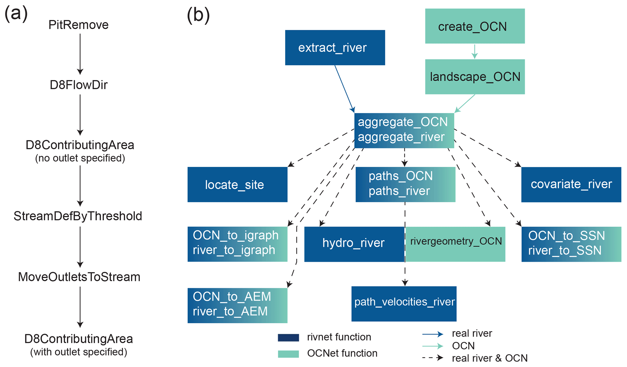
Figure 1(a) Sequence of TauDEM commands operated by extract_river. (b) Structure of the rivnet and OCNet packages. In both panels, arrows indicate that the output of a function is used as input of the next function.
In rivnet, river network extraction is performed via TauDEM's D8 flow algorithm, which allows for univocal determination of flow paths and along-stream distances. TauDEM command line executables are invoked via the traudem R package (Carraro et al., 2022), which provides an interface for the TauDEM methods and guides the installation of the TauDEM C library, as well as its dependencies GDAL (Geospatial Data Abstraction Library) and MPI (Message Passing Interface), depending on the operating system used. The main function of the rivnet package, extract_river, executes a fixed sequence of TauDEM commands to delineate the essential properties of a catchment, that is, flow directions and drainage areas (Fig. 1a). An optional parameter, threshold, can be passed to TauDEM's MoveOutletsToStream to tune the subset of pixels (of drainage area larger than threshold) to which the outlet is to be snapped, which thus enables a proper identification of the outlet location in the extracted stream network. In its simplest application, extract_river only requires the coordinates of the desired outlet(s) and a user-provided DEM or, alternatively, the extent of the region from which digital elevation data are to be downloaded, together with information on the coordinate system, i.e., the EPSG identifier of the Geodetic Parameter Dataset. In the latter case, control is passed to function get_elev_raster of elevatr for downloading the DEM data, prior to execution of the TauDEM commands.
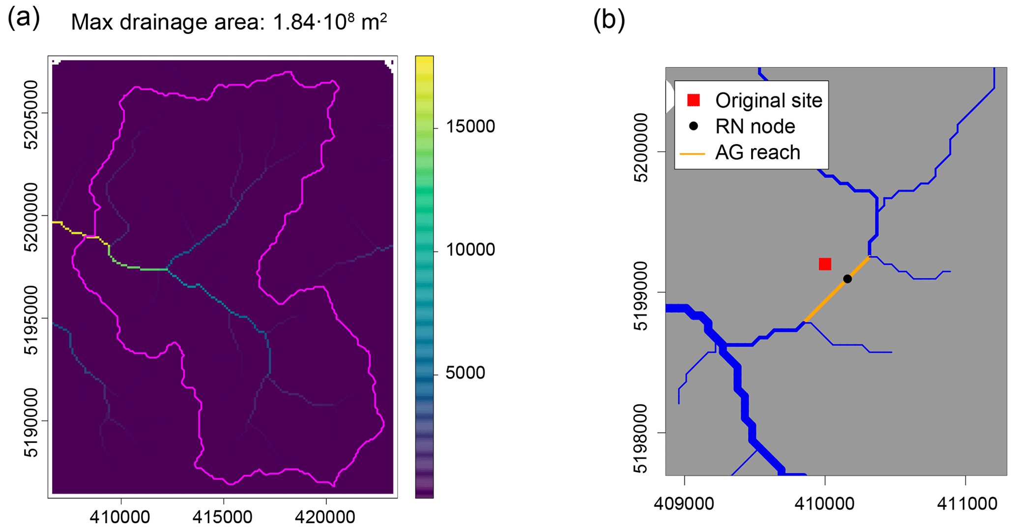
Figure 2Examples of drawing options in rivnet functions. (a) Use of option showPlot = TRUE in extract_river for the extraction of the river Ilfis (see Fig. 3). The color map indicates the number of cells drained by each cell, while the contour of the catchment extracted is displayed in magenta. Coordinates are given in the projected reference system ED50/UTM 32N (identified by option EPSG = 23 032). This can be used as a diagnostic tool in the case the extracted catchment is too small or does not have the expected shape. In such cases, it is suggested to tweak the outlet coordinates, option threshold or the DEM resolution. (b) Use of option showPlot = TRUE in locate_site for the same river of panel (a). A generic site (red square) is attributed to the closest river network (RN) and aggregated (AG) nodes (in this case, the distance as the crow flies is minimized).
Outputs from extract_river include an optional plot of the drainage area map and contour of the catchment corresponding to the selected outlet (which can be used as a diagnostic tool to assess whether the input outlet coordinates lead to the catchment sought after; Fig. 2a), a raster file of pit-filled elevations, D8 flow directions and drainage areas (in which case extract_river serves as a one-line wrapper for the sequence of TauDEM commands of Fig. 1a) and an object of the newly defined river S4 class. Such an object is compatible for use in the OCNet package, according to the scheme of Fig. 1b; river objects are de facto lists containing sublists (hence elements of river objects can be accessed with both “$” and “@” operators), which in turn define the river network at different aggregation levels. Carraro et al. (2020a) provides an extensive overview of definitions and use of aggregation levels, which are here briefly summarized for the sake of completeness. The flow direction (FD) level considers all DEM cells within the catchment as nodes of a network, and results from the application of extract_river. The so-obtained river object can be used as input into function aggregate_river, which mirrors aggregate_OCN of OCNet. This function defines three additional aggregation levels. The river network (RN) level is constituted by cells whose drainage area is larger than a given threshold value. A subset of such nodes then constitutes the aggregated (AG) level: in the simplest setting, these are constituted by source and confluence nodes. Properties at the AG level can either refer to the “node” (i.e., source or confluence cells) or the “edge” (i.e., the reach downstream of its associated node); for instance, reach length is provided for the edge, whereas drainage area values are provided with respect to both the node and the edge, in the latter case being equal to the drainage area at the downstream end of the reach. Additional nodes at the AG level can be included to split reaches that are excessively long (by imposing a maximum allowed reach length via option maxReachLength) or in correspondence with point features that the user might want to include in their model or design (say, a dam or a wastewater treatment plant); for this latter purpose, option breakpoints can be used in aggregate_river. Finally, each so-obtained reach is associated with a subcatchment (SC level), that is, the set of cells that directly drain into a reach.
Objects of the river class can be displayed using the plot() base function, which can call different drawing functions of OCNet depending on whether or not the object has been aggregated via aggregate_river and on optional themes to be displayed along the river network (see an example in Sect. 3). Aggregated river objects can be processed by paths_river (mirroring the analogous function from OCNet), which enables calculation of along-stream paths and distances between nodes at the RN and AG levels. Functions river_to_igraph and river_to_SSN mirror the corresponding functions of OCNet (Fig. 1b) and allow for porting river objects in alternative formats. Moreover, function river_to_AEM, mirroring an equivalent function from OCNet, provides an interface for the adespatial R package and allows for computing asymmetric eigenvector maps, that is, mutually orthogonal spatial variables obtained by a spatial filtering technique that considers space in an asymmetric way and are thus suitable to model species distributions in river networks (Blanchet et al., 2008).
Other functions have been specifically developed for the rivnet package and are aimed to provide relevant variables for use in ecohydrological and ecological applications. First, function covariate_river allows for evaluating covariate values at the subcatchment (SC) level from user-provided raster files. Covariates are calculated with reference to both local (i.e., average values across a subcatchment) and upstream reference areas, and can be either categorical (each cell of the input raster belongs to a different category, which is the case for land cover types) or continuous (for instance, mean air temperature at each cell). Covariate values calculated by covariate_river are the fraction of cells covered by a specific category within the reference area, or the mean value across cells within the reference area in the case of continuous inputs.
Second, function hydro_river provides a hydraulic geometry model for the whole river network based on well-established scaling relationships of hydraulic variables (Leopold and Maddock, 1953) and uniform flow relationships. The evaluated hydraulic variables (either at the RN or AG level) are river width, depth, water velocity, water volume, hydraulic radius and average bottom shear stress. The minimal necessary input is one value of width and one value of depth or discharge at two locations in the river network (which can but do not have to be the same location for both measures). Depending on the type and number of width, discharge and depth values provided as input, hydro_river can calculate hydraulic variables in different ways (see the package documentation for details). When both discharge and depth data are provided to the function, the preference for the use of power-law scaling relationships or uniform flow equation can be set by the user; if a uniform flow equation is used, the roughness coefficient can be made spatially varying. The function can handle cross-sections of different shapes, provided that they are vertically symmetric and that river width w can be expressed as a power law of depth d. This formulation includes rectangular, triangular and natural sections (for which w∼d0.65, according to Leopold and Maddock, 1953). While hydro_model assumes that the input hydraulic data are referred to the same time point (and hence the assignment of hydraulic variables across the network is a sort of spatial interpolation), the use of a non-rectangular cross-section allows for implementing variation in the width over time, which for instance is of interest when studying the role of hydrologic contraction on organic matter dynamics (Catalàn et al., 2023). If temporal variation in hydraulic variables is required, hydro_river should be applied separately for each time point.
Third, function path_velocities_river can be applied after paths (via paths_river) and hydraulic variables (via hydro_river) have been computed in order to calculate mean water velocities across any path between two connected nodes (either at the RN or AG level). These could be relevant for transport models, for instance in the case of environmental DNA (Carraro et al., 2020b). Finally, locate_site, unlike the previous functions, does not produce a river object but identifies the RN and AG nodes that are closest to a given point, either as the crow flies or along the downstream direction. Coordinates of such point need to be inputted manually but can be retrieved by clicking on a map via the locator() graphics function. Function locate_site also provides a drawing option, which plots a close-up of the river object in the area of interest, thus facilitating the correct identification of a site (Fig. 2b). This function allows for pinpointing the location of sampling sites across a river network, as well as other point features that might be included as nodes of the network (via the breakpoints argument of aggregate_river), but it can also be used to evaluate the distance of non-riverine sites to the river network (e.g., meteorological stations or plot sampling sites for ecological assessment).
From the perspective of a joint use with rivnet, several functions of OCNet have been expanded and improved. In particular, as of OCNet v0.6.0, the speed of aggregate_OCN has increased substantially (about 2 orders of magnitude faster than the previous version), draw_subcatchments_OCN allows for displaying themes across subcatchments, the plotting algorithm in draw_thematic_OCN has been made more agile and OCN_to_SSN allows for input of observation and predicted design from user-specified coordinates.
3.1 Scaling properties of river networks
A first case study focuses on the evaluation of widely known elongation and aggregation properties of river networks. In particular, Hack's law (Hack, 1957) states that the length L of the main river stem in a catchment scales as a power law of the drainage area A: L∼Ah, where superscript h is termed Hack's exponent and is expected to range between 0.45 and 0.7, with a value of 0.6 that is suitable for basins up to 20 000 km2 (Sassolas-Serrayet et al., 2018). Within a catchment, the probability distribution of drainage areas is also expected to follow a power law: , with (Rinaldo et al., 2014). The universality of interrelated power-law scaling relationships in drainage basins has been interpreted as the signature of the fractal character of river networks (Maritan et al., 1996). Performing such analysis in rivnet allows for showing how areas, along-stream and out-of-stream distances and different aggregation levels (RN, AG, SC) can be used.
Both Hack's law and the probability distribution of drainage areas were evaluated for four Swiss rivers of different total catchment areas (range: 185–5329 km2) extracted and analyzed via rivnet. Function extract_river was applied to a Mapzen open-source DEM with a cell resolution of about 50 m (the exact resolution depends on the latitude; see the documentation of elevatr for details). To evaluate Hack's law, the procedure described in Sassolas-Serrayet et al. (2018) was followed: a threshold area of 1 km2 was used in aggregate_river to evaluate the network nodes at the AG level. Confluence nodes were used as sub-basin outlets where upstream areas A and lengths L were evaluated. Upstream lengths are made up of an along-stream component (evaluated via paths_river), i.e., the distance from the considered sub-basin outlet to a source node, and an out-of-stream component evaluated as the horizontal distance from a source node to the subcatchment divide (Sassolas-Serrayet et al., 2018). The relationship between L and A for the four analyzed rivers is shown in Fig. 3a. Values of the Hack's exponent found for the four analyzed basins are within the expected range (Fig. 3a). The power-law scaling of drainage areas is also verified (Fig. 3b), with exponents that are in fair agreement with theoretical values (Rodríguez-Iturbe and Rinaldo, 2001).
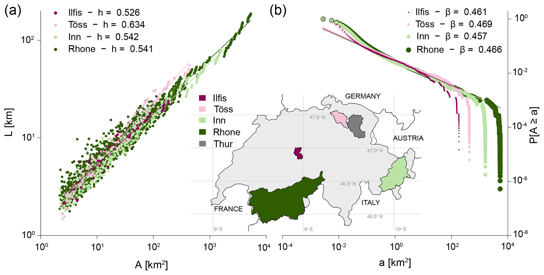
Figure 3Results of the case study on scaling properties of river networks. (a) Scaling of length of the main river stem L with drainage area A (Hack's law): L∼Ah. Fitted Hack's exponent values for the four analyzed basins are reported in the legend. (b) Probability distribution of drainage areas . Fitted exponent values are reported in the legend. The inset displays the location of the four analyzed basins within Switzerland, as well as the Thur catchment (Fig. 5).
This case study also allows for assessment of the computational performance of rivnet. As shown in Fig. 4, a relevant portion of the total computational time needed to produce the river objects used in this application is spent on DEM download and execution of TauDEM commands, while the total overhead required by functions extract_river, aggregate_river and paths_river is of the same order of magnitude as the two aforementioned tasks.
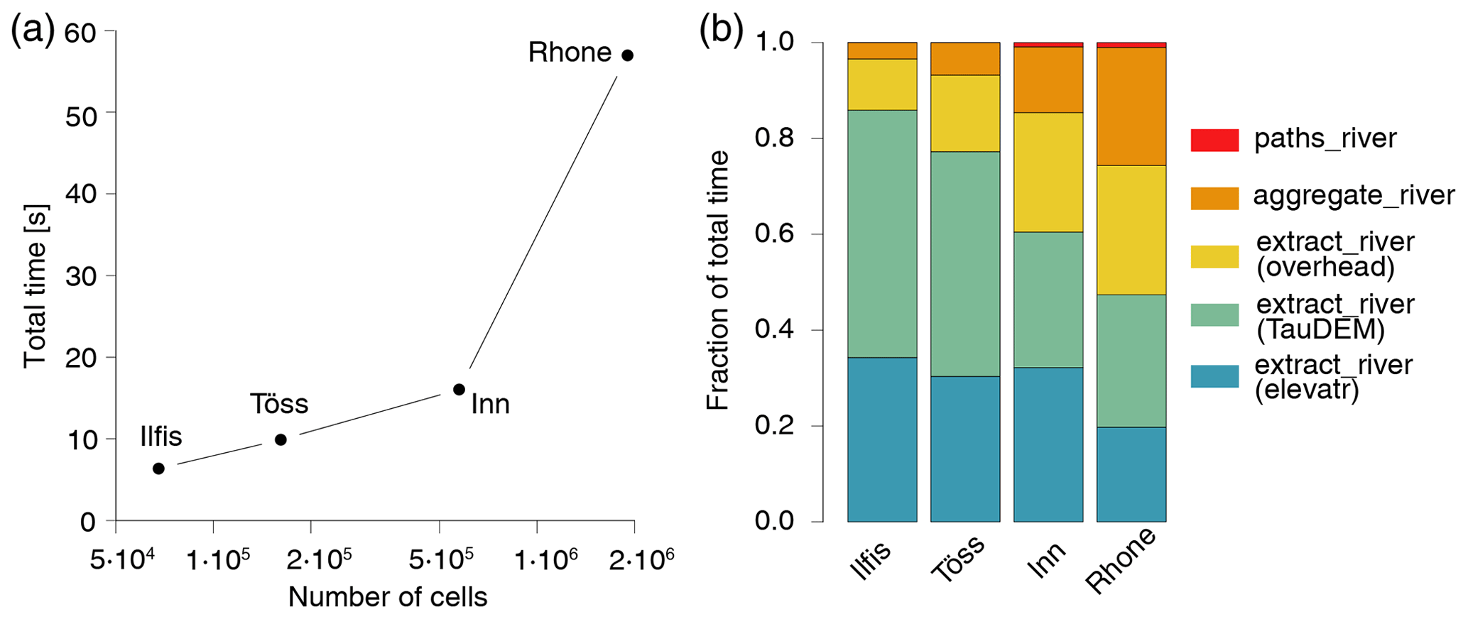
Figure 4Estimates of computational time needed to produce the river objects used in the analysis of Fig. 3. (a) Total time required as a function of the number of cells in the catchment. (b) Breakdown of time for the different rivnet functions used: in particular, the time spent by extract_river is partitioned into time required by DEM downloading (“elevatr”), application of TauDEM commands (“TauDEM”) and creation of a river object (“overhead”). Results are the average of five runs operated via an Intel® quad core i7-7700K processor with 16 GB RAM; TauDEM commands were run with eight parallel processors.
3.2 Release and transport of phosphorous at a catchment scale
The second case study applies a model of phosphorous dynamics to a Swiss river making use of rivnet functions. The model essentially follows Yang et al. (2021b), and it constitutes a component of the CnANDY (Coupled, Complex Algal-Nutrient DYnamics) model aimed at a parsimonious representation of dynamics of benthic and pelagic algae across a river network and their interaction with a single limiting nutrient (phosphorous). In particular, this exercise illustrates the use of rivnet functions to calculate covariate values (covariate_river), assign hydraulic variables (hydro_river) and pinpoint sites on the river network (locate_site).
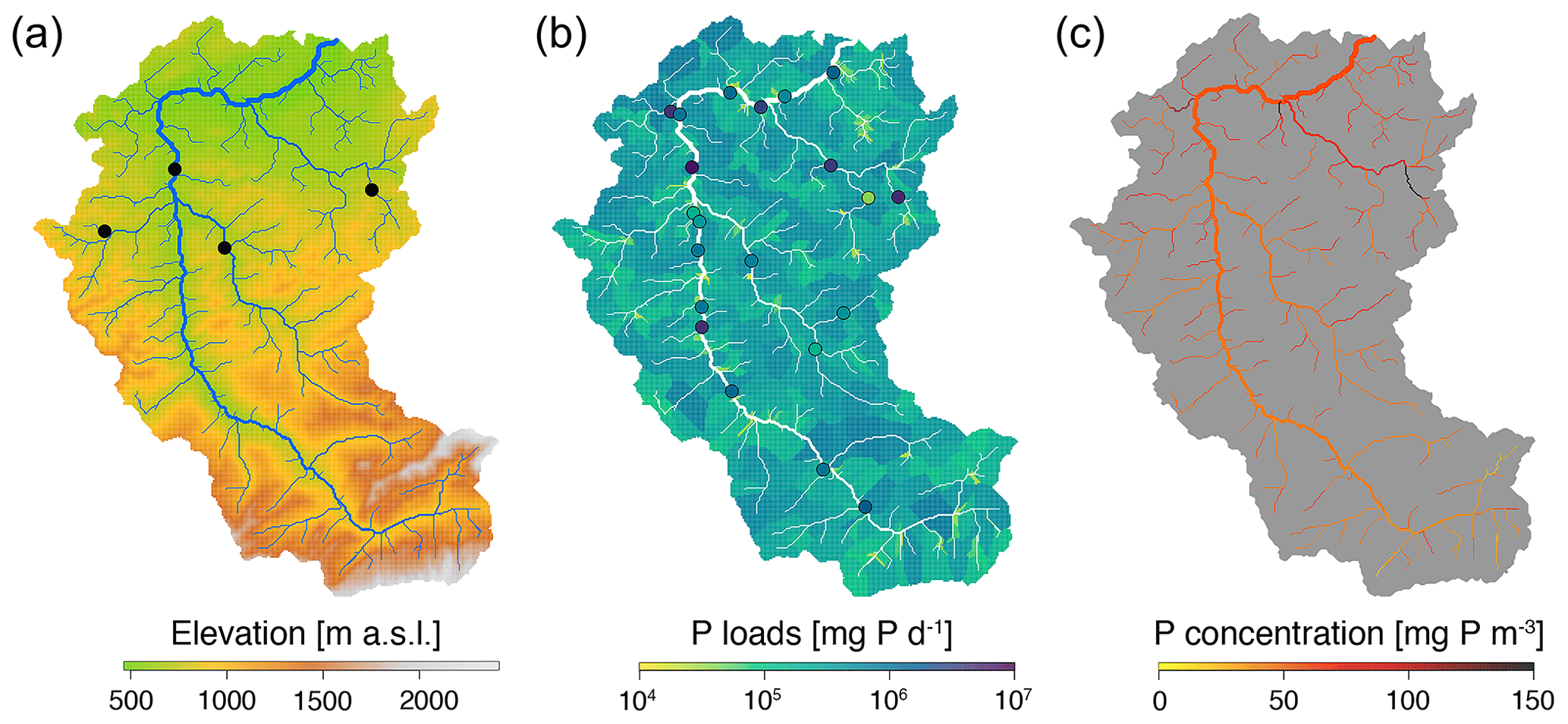
Figure 5Results of the case study on phosphorous release and transport. (a) Elevation map of the Thur catchment. Black dots indicate the locations of the hydrological stations. (b) Map of phosphorous loads: diffuse loads ϕD,i are color-coded on the respective subcatchments, while point loads ϕP,i are displayed as dots. (c) Map of phosphorous concentration as predicted by the model (Eq. 1). The three panels were obtained as specific cases of the plot() function.
According to Yang et al. (2021b), phosphorous inputs to the stream are related to both diffuse (i.e., depending on the different land use types) and point (i.e., related to wastewater treatment plants – WWTPs) sources and are indicated with ϕD,i and ϕP,i [g P d−1], respectively, where subscript i indicates a given reach (node at the AG level) of the network. Phosphorous is assumed to be advected by streamflow while processed by the microbial community. The model reads
where Pi [g P] is the phosphorous mass in reach i; wji is an element of the adjacency matrix (equal to 1 if node j drains into i and null otherwise); Qi [m3 s−1], Vi [m3] and di [m] are the water discharge, water volume and river depth in reach i, respectively; and vf [m s−1] is an uptake velocity accounting for transformation processes operated by microbial biofilm in the hyporheic zone (Basu et al., 2011). Point phosphorous loads were estimated as , where kP [g P d−1] is the phosphorous load per equivalent inhabitant and Hi the population equivalent of the WWTP located in reach i. Diffuse loads were estimated based on three main land cover types (forested, agricultural and urban areas) as , where AS,i [m2] is the area of the subcatchment pertaining to reach i; fF,i, fA,i and fU,i are the fractions of AS,i covered by forested, agricultural and urban areas, respectively; and kF, kA and kU [mg P m−2 d−1] are their respective phosphorous loads per unit area.
Model Eq. (1) was applied to evaluate steady-state phosphorous concentrations in a Swiss catchment (the Thur, Figs. 3b and 5a), which is known to have very different environmental conditions among its main tributaries (Carraro et al., 2020b). The river network was extracted via extract_river from the same DEM as in the previous application and was aggregated (via aggregate_river) to a total of 413 nodes at the AG level by imposing a threshold area of 1 km2 and a maximum reach length of 2500 m. Data on WWTPs and a raster land cover map for Switzerland were retrieved from open-source databases of the Swiss Federal Office for the Environment (FOEN). A total of 21 WWTPs are present in the Thur catchment (Fig. 5b); their attribution to the AG nodes of the river network was performed via locate_site, while covariate_river was used to evaluate fF,i, fA,i and fU,i. Four hydrological stations operated by FOEN are located within the catchment (Fig. 5a); their corresponding AG nodes were assessed via locate_site. At these locations, river width was estimated via aerial images, and mean water discharges in the period 2012–2021 were calculated from the FOEN data. Function hydro_river was used with such inputs to assign hydraulic variables across the network, by assuming uniform flow conditions and a spatially constant Gauckler–Strickler roughness coefficient equal to 30 m s−1, and natural river cross-sections. Model parameters were taken as in Yang et al. (2021b): vf=0.17 m d−1, kP=150 mg P d−1 (per inhabitant), kF=0.1 mg P m−2 d−1, kA=0.15 mg P m−2 d−1 and kU=0.3 mg P m−2 d−1. Phosphorous concentrations predicted by Eq. (1) are shown in Fig. 5c. The highest phosphorous loads are observed in the north-eastern part of the Thur catchment, in correspondence with a large WWTP located in a small reach (Fig. 5b).
The rivnet package enables the analysis of river networks in the R environment with a particular emphasis on environmental modeling purposes. Being based on digital elevation data (rather than river shapefiles), it allows for computation of areas and thus attribution of covariate values or hydraulic variables across a river network. Extraction of drainage patterns is based on TauDEM's D8 flow direction algorithm, a robust and widely used method that allows for univocal evaluation of distances between stream sites. A major asset of rivnet is that, unlike other DEM-based river network analysis tools, it does not require the use of graphical user interface-based GIS software, and hence it allows for replicable workflows while at the same time providing a series of drawing options and functions assisting in tasks such as delineating the catchment shape or localizing a site within a river. The use of a fixed sequence of TauDEM commands is advantageous because it makes the task of extracting a river network accessible to users unfamiliar with geomorphologic, hydrologic or GIS tools. In the same spirit, rivnet functions are designed so as to require a minimal amount of user input: by interfacing with the elevatr package, it is sufficient to provide the extent of the region of interest and outlet coordinates in order to obtain river data, and minimal information on river hydraulics (say, one width and one discharge value) is enough to produce a hydraulic model for the whole river network. At the same time, a wide set of options enables customization for more experienced users. Moreover, river objects can be exported in free format, thus allowing for subsequent landscape analyses with D-infinity or other methods and software.
The main limitations of the rivnet package are inherent to the use of the D8 method. In particular, being based on DEM analysis, the accuracy of the determination of flow directions is constrained by the quality of the topographic data provided. This implies that river network delineation in low-relief areas could be imprecise, as algorithms specifically tailored for flat landscapes (e.g., Passalacqua et al., 2012) are not included in the current workflow. To help overcome this limitation, as well as those induced by artificial flow paths (such as ditches or pipes across elevation boundaries), it is thus suggested to manually decrease the elevation of the affected cells in the input DEM. Additionally, the use of a single flow direction algorithm such as D8 does not allow for handling braided channels. In fact, TauDEM's D8 method, and in turn the rivnet package, is aimed towards catchment-scale terrain analysis, and hence topographic features at a reach scale might not be accurately reproduced.
In conclusion, because of its simplicity and wide range of possible applications, rivnet can facilitate and promote the development of spatially explicit ecological and biogeochemical models in river networks, which are crucial tools for a mechanistic understanding of the state and change in freshwater environments.
The rivnet package is available on CRAN at the following link: https://CRAN.R-project.org/package=rivnet (Carraro, 2023a). Scripts reproducing the applications are available at the following link: https://doi.org/10.5281/zenodo.8279240 (Carraro, 2023b). Data used in the applications are freely accessible online (links are provided in the aforementioned scripts).
The author has declared that there are no competing interests.
Publisher's note: Copernicus Publications remains neutral with regard to jurisdictional claims made in the text, published maps, institutional affiliations, or any other geographical representation in this paper. While Copernicus Publications makes every effort to include appropriate place names, the final responsibility lies with the authors.
The author thanks Florian Altermatt, Enrico Bertuzzo and François Keck for their helpful comments and feedback on the package and article.
This research has been supported by the Schweizerischer Nationalfonds zur Förderung der Wissenschaftlichen Forschung (Ambizione grant no. PZ00P2_202010).
This paper was edited by Roger Moussa and reviewed by Polina Lemenkova and Warrick Dawes.
Altermatt, F.: Diversity in riverine metacommunities: A network perspective, Aquat. Ecol., 47, 365–377, https://doi.org/10.1007/s10452-013-9450-3, 2013. a
Amatulli, G., Garcia Marquez, J., Sethi, T., Kiesel, J., Grigoropoulou, A., Üblacker, M. M., Shen, L. Q., and Domisch, S.: Hydrography90m: a new high-resolution global hydrographic dataset, Earth Syst. Sci. Data, 14, 4525–4550, https://doi.org/10.5194/essd-14-4525-2022, 2022. a
Baldan, D., Cunillera-Montcusí, D., Funk, A., and Hein, T.: Introducing `riverconn': an R package to assess river connectivity indices, Environ. Model. Softw., 156, 105470, https://doi.org/10.1016/j.envsoft.2022.105470, 2022. a, b
Basu, N. B., Rao, P. S. C., Thompson, S. E., Loukinova, N. V., Donner, S. D., Ye, S., and Sivapalan, M.: Spatiotemporal averaging of in-stream solute removal dynamics, Water Resour. Res., 47, W00J06, https://doi.org/10.1029/2010WR010196, 2011. a
Bertuzzo, E., Casagrandi, R., Gatto, M., Rodríguez-Iturbe, I., and Rinaldo, A.: On spatially explicit models of cholera epidemics, J. Roy. Soc. Interf., 7, 321–333, https://doi.org/10.1098/rsif.2009.0204, 2010. a
Beven, K. and Freer, J.: A dynamic TOPMODEL, Hydrol. Process., 15 1993–2011, https://doi.org/10.1002/hyp.252, 2001. a
Blanchet, F. G., Legendre, P., and Borcard, D.: Modelling directional spatial processes in ecological data, Ecol. Model., 215, 325–336, https://doi.org/10.1016/j.ecolmodel.2008.04.001, 2008. a
Blöschl, G. and Sivapalan, M.: Scale issues in hydrological modelling: A review, Hydrol. Process., 9, 251–290, 1995. a
Buisson, L., Blanc, L., and Grenouillet, G.: Modelling stream fish species distribution in a river network: the relative effects of temperature versus physical factors, Ecol. Freshw. Fish, 17, 244–257, https://doi.org/10.1111/j.1600-0633.2007.00276.x, 2008. a
Carraro, L.: rivnet: Extract and Analyze Rivers from Elevation Data, R package version 0.3.2, CRAN [code], https://CRAN.R-project.org/package=rivnet (last access: 19 October 2023), 2023a. a
Carraro, L.: test_rivnet: v1.0, Zenodo [code], https://doi.org/10.5281/zenodo.8279240, 2023b. a
Carraro, L. and Altermatt, F.: Optimal Channel Networks accurately model ecologically-relevant geomorphological features of branching river networks, Commun. Earth Environ., 3, 125, https://doi.org/10.1038/s43247-022-00454-1, 2022. a
Carraro, L., Bertuzzo, E., Mari, L., Fontes, I., Hartikainen, H., Strepparava, N., Schmidt-Posthaus, H., Wahli, T., Jokela, J., Gatto, M., and Rinaldo, A.: Integrated field, laboratory, and theoretical study of PKD spread in a Swiss prealpine river, P. Natl. Acad. Sci. USA, 114, 11992–11997, 2017. a
Carraro, L., Hartikainen, H., Jokela, J., Bertuzzo, E., and Rinaldo, A.: Estimating species distribution and abundance in river networks using environmental DNA, P. Natl. Acad. Sci. USA, 115, 11724–11729, 2018. a
Carraro, L., Bertuzzo, E., Fronhofer, E. A., Furrer, R., Gounand, I., Rinaldo, A., and Altermatt, F.: Generation and application of river network analogues for use in ecology and evolution, Ecol. Evol., 10, 7537–7550, https://doi.org/10.1002/ece3.6479, 2020a. a, b
Carraro, L., Mächler, E., Wüthrich, R., and Altermatt, F.: Environmental DNA allows upscaling spatial patterns of biodiversity in freshwater ecosystems, Nat. Commun., 11, 3585, https://doi.org/10.1038/s41467-020-17337-8, 2020b. a, b
Carraro, L., Toffolon, M., Rinaldo, A., and Bertuzzo, E.: SESTET: A spatially explicit stream temperature model based on equilibrium temperature, Hydrol. Process., 34, 355–369, 2020c. a
Carraro, L., Salmon, M., Sadek, W., and Müller, K.: traudem: Use TauDEM, r package version 1.0.1, https://CRAN.R-project.org/package=traudem (last access: 19 October 2023), 2022. a
Catalàn, N., Campo, R. D., Talluto, M., Mendoza-Lera, C., Grandi, G., Bernal, S., Schiller, D. V., Singer, G., and Bertuzzo, E.: Pulse, Shunt and Storage: Hydrological Contraction Shapes Processing and Export of Particulate Organic Matter in River Networks, Ecosystems, 26, 873–892, https://doi.org/10.1007/s10021-022-00802-4, 2023. a
Csardi, G. and Nepusz, T.: The igraph software package for complex network research, InterJournal, Complex Syst., 1695, 1–9, 2006. a, b
Czuba, J. A.: A Lagrangian framework for exploring complexities of mixed-size sediment transport in gravel-bedded river networks, Geomorphology, 321, 146–152, 2018. a
David, S. R., Murphy, B. P., Czuba, J. A., Ahammad, M., and Belmont, P.: USUAL Watershed Tools: A new geospatial toolkit for hydro-geomorphic delineation, Environ. Model. Soft., 159, 105576, https://doi.org/10.1016/j.envsoft.2022.105576, 2023. a, b
Domisch, S., Amatulli, G., and Jetz, W.: Near-global freshwater-specific environmental variables for biodiversity analyses in 1 km resolution, Scient. Data, 2, 1–13, 2015. a
Florinsky, I. V., Eilers, R. G., Manning, G., and Fuller, L.: Prediction of soil properties by digital terrain modelling, Environ. Model. Softw., 17, 295–311, 2002. a
Frissell, C. A., Liss, W. J., Warren, C. E., and Hurley, M. D.: A hierarchical framework for stream habitat classification: viewing streams in a watershed context, Environ. Manage., 10, 199–214, 1986. a
Hack, J. T.: Studies of longitudinal stream profiles in Virginia and Maryland, US Geological Survey Professional Paper B 294, US Geological Survey, 1–97, 1957. a
Hollister, J., Shah, T., Robitaille, A. L., Beck, M. W., and Johnson, M.: elevatr: Access Elevation Data from Various APIs, R package version 0.99.0, https://CRAN.R-project.org/package=elevatr/ (last access: 19 October 2023), 2023. a
Jacquet, C., Carraro, L., and Altermatt, F.: Meta-ecosystem dynamics drive the spatial distribution of functional groups in river networks, Oikos, 2022, e09372, https://doi.org/10.1111/oik.09372, 2022. a
Kattwinkel, M., Szöcs, E., Peterson, E., and Schäfer, R. B.: Preparing GIS data for analysis of stream monitoring data: The R package openSTARS, Plos One, 15, e0239237, https://doi.org/10.1371/journal.pone.0239237, 2020. a
Kenward, T., Lettenmaier, D. P., Wood, E. F., and Fielding, E.: Effects of digital elevation model accuracy on hydrologic predictions, Remote Sens. Environ., 74, 432–444, 2000. a
Leopold, L. B. and Maddock, T. The hydraulic geometry of stream channels and some physiographic implications, US Geological Survey Professional Paper 252, US Geological Survey, 1–97, https://doi.org/10.3133/pp252, 1953. a, b
Lois, S., Cowley, D. E., Outeiro, A., San Miguel, E., Amaro, R., and Ondina, P.: Spatial extent of biotic interactions affects species distribution and abundance in river networks: The freshwater pearl mussel and its hosts, J. Biogeogr., 42, 229–240, 2015. a
Lyu, F., Xu, Z., Ma, X., Wang, S., Li, Z., and Wang, S.: A vector-based method for drainage network analysis based on LiDAR data, Comput. Geosci., 156, 104892, https://doi.org/10.1016/j.cageo.2021.104892, 2021. a
Marani, A., Rigon, R., and Rinaldo, A.: A Note on Fractal Channel Networks, Water Resour. Res., 27, 3041–3049, https://doi.org/10.1029/91WR02077, 1991. a
Maritan, A., Rinaldo, A., Rigon, R., Giacometti, A., and Rodríguez-Iturbe, I.: Scaling laws for river networks, Phys. Rev. E, 53, 1510–1515, https://doi.org/10.1103/PhysRevE.53.1510, 1996. a, b
O'Callaghan, J. F. and Mark, D. M.: The extraction of drainage networks from digital elevation data, Comput. Vis. Graph. Image Process., 28, 323–344, https://doi.org/10.1016/S0734-189X(84)80011-0, 1984. a
Passalacqua, P., Belmont, P., and Foufoula-Georgiou, E.: Automatic geomorphic feature extraction from lidar in flat and engineered landscapes, Water Resour. Res., 48, W03528, https://doi.org/10.1029/2011WR010958, 2012. a
Quinn, P., Beven, K., Chevallier, P., and Planchon, O.: The prediction of hillslope flow paths for distributed hydrological modelling using digital terrain models, Hydrol. Process., 5, 59–79, https://doi.org/10.1002/hyp.3360050106, 1991. a
Reichert, P.: rivernet: Read, Analyze and Plot River Networks, r package version 1.2.3, https://CRAN.R-project.org/package=rivernet (last access: 19 October 2023), 2020. a
Rinaldo, A., Rigon, R., Banavar, J. R., Maritan, A., and Rodríguez-Iturbe, I.: Evolution and selection of river networks: Statics, dynamics, and complexity, P. Natl. Acad. Sci., 111, 2417–2424, https://doi.org/10.1073/pnas.1322700111, 2014. a
Rodríguez-Iturbe, I. and Rinaldo, A.: Fractal River Basins. Chance and self-organization, Cambridge University Press, New York, USA, ISBN 9780521004053, 2001. a, b
Rodríguez-Iturbe, I., Ijjász‐Vásquez, E. J., Bras, R. L., and Tarboton, D. G.: Power law distributions of discharge mass and energy in river basins, Water Resour. Res., 28, 1089–1093, https://doi.org/10.1029/91WR03033, 1992. a
Sassolas-Serrayet, T., Cattin, R., and Ferry, M.: The shape of watersheds, Nat. Commun., 9, 3791, https://doi.org/10.1038/s41467-018-06210-4, 2018. a, b, c
Schwanghart, W. and Kuhn, N. J.: TopoToolbox: A set of Matlab functions for topographic analysis, Environ. Model. Softw., 25, 770–781, https://doi.org/10.1016/j.envsoft.2009.12.002, 2010. a
Segatto, P. L., Battin, T. J., and Bertuzzo, E.: The Metabolic Regimes at the Scale of an Entire Stream Network Unveiled Through Sensor Data and Machine Learning, Ecosystems, 24, 1792–1809, 2021. a
Segatto, P. L., Battin, T. J., and Bertuzzo, E.: A Network-Scale Modeling Framework for Stream Metabolism, Ecosystem Efficiency and Their Response to Climate Change, Water Resour. Res., 59, e2022WR034062, https://doi.org/10.1029/2022WR034062, 2023. a
Tarboton, D. G.: A new method for the determination of flow directions and upslope areas in grid digital elevation models, Water Resour. Res., 33, 309–319, 1997. a, b
Tarboton, D. G., Bras, R. L., and Rodriguez‐Iturbe, I.: On the extraction of channel networks from digital elevation data, Hydrol. Process., 5, 81–100, 1991. a
Tonkin, J. D., Altermatt, F., Finn, D. S., Heino, J., Olden, J. D., Pauls, S. U., and Lytle, D. A.: The role of dispersal in river network metacommunities: Patterns, processes, and pathways, Freshwater Biol., 63, 141–163, https://doi.org/10.1111/fwb.13037, 2018. a
Tyers, M.: riverdist: River Network Distance Computation and Applications, r package version 0.16.1, https://CRAN.R-project.org/package=riverdist (last access: 19 October 2023), 2022. a
Uzun, P., Farazande, S., and Guven, B.: Mathematical modeling of microplastic abundance, distribution, and transport in water environments: a review, Chemosphere, 288, 132517, https://doi.org/10.1016/j.chemosphere.2021.132517, 2022. a
Vannote, R. L., Minshall, G. W., Cummins, K. W., Sedell, J. R., and Cushing, C. E.: The river continuum concept, Can. J. Fish. Aquat. Sci., 37, 130–137, https://doi.org/10.1139/f80-017, 1980. a
Ver Hoef, J. M., Peterson, E. E., Cliord, D., and Shah, R.: SSN: An R package for spatial statistical modeling on stream networks, J. Stat. Softw., 56, 1–45, 2014. a, b
Wang, L. and Ai, T.: The Comparison Of Drainage Network Extraction Between Square And Hexagonal Grid-based DEM, The International Archives of the Photogrammetry, Remote Sens. Spat. Inform. Sci., XLII-4, 687–692, https://doi.org/10.5194/isprs-archives-XLII-4-687-2018, 2018. a
Wu, T., Li, J., Li, T., Sivakumar, B., Zhang, G., and Wang, G.: High-efficient extraction of drainage networks from digital elevation models constrained by enhanced flow enforcement from known river maps, Geomorphology, 340, 184–201, https://doi.org/10.1016/j.geomorph.2019.04.022, 2019. a
Yang, S., Bertuzzo, E., Borchardt, D., and Rao, P. S. C.: Hortonian Scaling of Coupled Hydrological and Biogeochemical Responses Across an Intensively Managed River Basin, Front. Water, 3, https://doi.org/10.3389/frwa.2021.693056, 2021a. a
Yang, S., Bertuzzo, E., Büttner, O., Borchardt, D., and Rao, P. S. C.: Emergent spatial patterns of competing benthic and pelagic algae in a river network: A parsimonious basin-scale modeling analysis, Water Res., 193, 116887, https://doi.org/10.1016/j.watres.2021.116887, 2021b. a, b, c
Zhang, W. and Montgomery, D. R.: Digital elevation model grid size, landscape representation, and hydrologic simulations, Water Resour. Res., 30, 1019–1028, 1994. a