Technical note: NASAaccess – a tool for access, reformatting, and visualization of remotely sensed earth observation and climate data

The National Aeronautics and Space Administration (NASA) has launched a new initiative, the Open-Source Science Initiative (OSSI), to enable and support science towards openness. The OSSI supports open-source software development and dissemination. In this work, we present NASAaccess, which is an open-source software package and web-based environmental modeling application for earth observation data accessing, reformatting, and presenting quantitative data products. The main objective of developing the NASAaccess platform is to facilitate exploration, modeling, and understanding of earth data for scientists, stakeholders, and concerned citizens whose objectives align with the new OSSI goals. The NASAaccess platform is available as software packages (i.e., the R and conda packages) as well as an interactive-format web-based environmental modeling application for earth observation data developed with Tethys Platform. NASAaccess has been envisioned as lowering the technical barriers and simplifying the process of accessing scalable distributed computing resources and leveraging additional software for data and computationally intensive modeling frameworks. Specifically, NASAaccess has been developed to meet the need for seamless earth observation remote-sensing and climate data ingestion into various hydrological modeling frameworks. Moreover, NASAaccess is also contributing to keeping interested parties and stakeholders engaged with environmental modeling, accessing the information available in various remote-sensing products. NASAaccess' current capabilities cover various NASA datasets and products that include the Global Precipitation Measurement (GPM) data products, the Global Land Data Assimilation System (GLDAS) land surface states and fluxes, and the NASA Earth Exchange Global Daily Downscaled Projections (NEX-GDDP) Coupled Model Intercomparison Project Phase 5 (CMIP5) and Coupled Model Intercomparison Project Phase 6 (CMIP6) climate change dataset products.

1 Introduction

One of the key elements of a paradigm shift in hydrologic science as outlined by Wagener et al. (2010) is that real-time learning observations, modeling, and management are interactive exercises with feedback and updating. Recently, sharing data, code, and other research products has become more common but is still not a popular practice. That is because there are few incentives for preparing datasets and code for sharing, and this may even be discouraged by current programs and agencies who are hesitant to support data-sharing platforms. This is one of the limitations to the progress of science as discussed by a recent National Academies of Sciences, Engineering, and Medicine report (National Academies of Sciences Engineering and Medicine, 2018).

Xu et al. (2022) presented an overview of visual computing applications developed for water resources management. These numerous applications have led to the emergence of innovative big data applications that can address past challenges and generate useful insights in water science disciplines (Talia et al., 2016). Xu et al. (2022) noted that many past visual computing applications developed for water resources management integrated visual computing techniques into the Geographic Information System (GIS), cyberinfrastructure, and domain models to benefit the big data analysis aspect of water resources management. These new visual computing techniques and features then become effective tools for disseminating water education, raising public awareness of various water problems and increasing public engagement. For instance, the Enhancing National Climate Services (ENACTS) initiative led by Columbia University's International Research Institute for Climate and Society (IRI) has been making efforts to disseminate climate information and support developing countries' decision-makers and stakeholders in making climate-sensitive economic activities more resilient to current climate extremes and adapting to the changing climate (Nsengiyumva et al., 2021). ENACTS is an initiative developed to alleviate the challenges of climate data availability as well as access and use by supporting countries to generate high-resolution gridded climate data time series and derived climate information products that are readily accessible to decision-makers (Dinku et al., 2014, 2018).

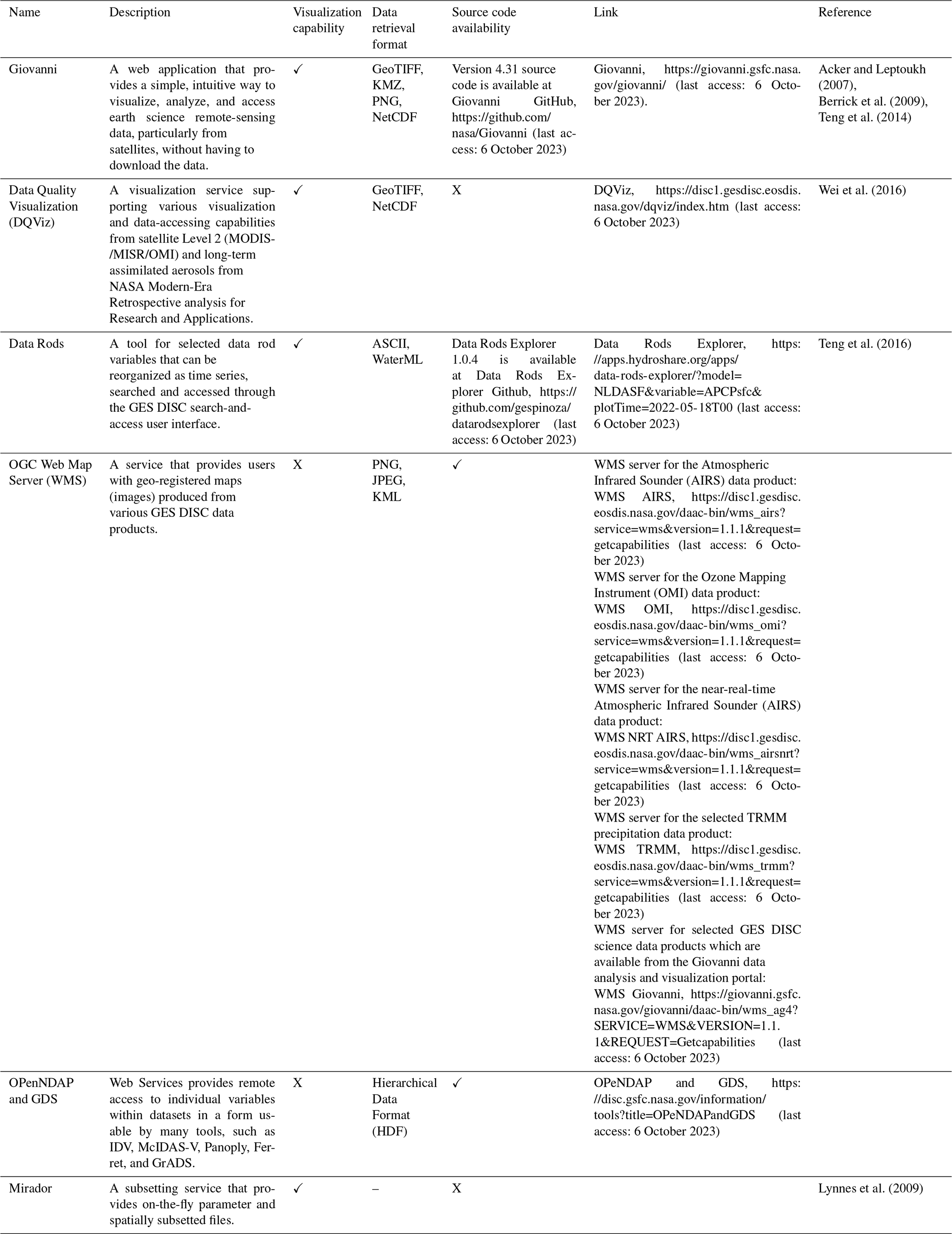
Earth science data observations are archived at the NASA Goddard Earth Sciences Data and Information Services Center (GES DISC) and other NASA data centers. The data observations are primarily organized as time-step arrays and in several common formats that support the creation, access, and sharing of array-oriented scientific data (e.g., HDF, netCDF). Ongoing work has been done over the years to facilitate access to, use of, and meeting of the need for NASA data by providing tools and services for data visualization, subsetting, and format conversion. In Table 1, we summarize a few NASA GES DISC tools and services that have been developed to meet growing needs and applications expressed by users for remote-sensing earth observation data.

Table 1 Selected NASA GES DISC tools and services for accessing and visualizing earth observation remote-sensing data.

NASA has launched a new initiative, the Open-Source Science Initiative (OSSI), to enable and support science towards openness (https://science.nasa.gov/open-science-overview, last access: 6 October 2023). The OSSI supports open-source software development and dissemination. To help meet challenges to the progress of science in earth observation data access and management, more tools need to be available, accessible, and understandable. This paper describes an open-source platform, e.g., the NASAaccess package, to access and present quantitative remote-sensing earth observation and climate data products in an interactive format so that scientists, stakeholders, and concerned citizens can engage in the exploration, modeling, and understanding of the data. The NASAaccess platform is available as R (R Development Core Team, 2022) and conda (https://docs.conda.io/en/latest/, last access: 6 October 2023) software packages as well as an interactive-format web-based environmental modeling application for earth observation data developed in the Tethys Platform framework (Swain et al., 2016). NASAaccess is envisaged as lowering the technical barrier and simplifying the process of accessing scalable distributed computing resources and leveraging a wide array of satellite-based earth observations for more comprehensive computationally intensive modeling frameworks. Specifically, NASAaccess has been developed to meet the need for seamless earth observation remote-sensing and climate data ingestion into other modeling frameworks, including Variable Infiltration Capacity (VIC) (Liang et al., 1994), the Distributed Hydrology Soil Vegetation Model (DHSVM) (Wigmosta et al., 1994), the Regional Hydro-Ecologic Simulation System (RHESSys) model (Tague and Band, 2004), and the Soil and Assessment Water Tool (SWAT) (Arnold and Fohrer, 2005). Moreover, NASAaccess is also contributing to keeping interested parties and stakeholders engaged with environmental modeling, accessing the information available in various remote-sensing products.

2 Methodology

2.1 NASAaccess key functionalities

The current NASAaccess (v.3.3.0) capabilities cover various NASA datasets and products that include the Global Precipitation Measurement (GPM) data products (Huffman et al., 2019), the Global Land Data Assimilation System (GLDAS) land surface states and fluxes (Rodell et al., 2004), and the NASA Earth Exchange Global Daily Downscaled Projections (NEX-GDDP) Coupled Model Intercomparison Project Phase 5 (CMIP5) (Wood et al., 2002, 2004; Maurer and Hidalgo, 2008; Thrasher et al., 2012) and Coupled Model Intercomparison Project Phase 6 (CMIP6) (Thrasher et al., 2022) climate change dataset products. A brief description is given for the current NASAaccess (v.3.3.0) function capabilities in Fig. 1. In principle, the functionality of NASAaccess can be summarized as follows.

• a.

  Accessing NASA servers to download earth observation data by fetching specific data for a specific domain and period.

• b.

  Clipping the needed data grids to an input shapefile of a user study watershed.

• c.

  Handling any temporal (i.e., processing diurnal minimum and maximum air temperatures from hourly input data) or spatial (e.g., finding the data that correspond to the study area centroid) inconsistencies.

• d.

  Generating gridded data files and definition files compatible with the various hydrological models (i.e., ASCII format).

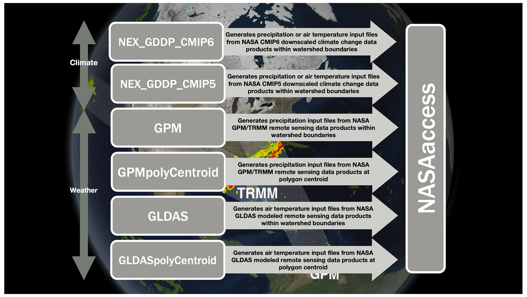
Figure 1 NASAaccess available functions (NASAaccess version 3.3.0). The map shows rain data collected by the GPM Core Observatory and the partner satellites currently in orbit on 17 March 2014 (NASA's Scientific Visualization Studio, https://svs.gsfc.nasa.gov/4203, last access: 6 October 2023).

2.2 NASAaccess package requirements

The NASAaccess package needs Earthdata login credentials (NASA Earthdata Login, https://urs.earthdata.nasa.gov/, last access: 6 October 2023) to be operable. Earthdata is a user registration and user profile management system for users getting earth science data from any of the Distributed Active Archive Centers (DAACs) that comprise NASA's Earth Observing System Data and Information System (EOSDIS). The NASAaccess package relies on the “curl” tool to transfer data from NASA servers to a user machine, using an HTTPS-supported protocol. The curl package (curl GitHub, https://github.com/jeroen/curl, last access: 6 October 2023) provides bindings to the libcurl C library for the R software program (R Development Core Team, 2022). The curl package supports retrieving data in-memory, downloading to disk, or streaming using the R “connection” interface. The curl command embedded in NASAaccess is designed to work seamlessly by appending appropriate login information to the “.netrc” file and the cookies file “.urs_cookies” to fetch various data products. The .netrc and .urs_cookies files need to be stored in the user's local directory before running any NASAaccess function; otherwise, the requested data will not be retrieved. Further details on how to make the curl tool work with the NASAaccess package and how to create the .netrc file and the .urs_cookies file can be reviewed on the NASAaccess Open Science Framework (OSF) wiki pages at Mohammed (2023a).

2.3 Tethys application framework

Tethys Platform (Swain et al., 2015, 2016) is a development and hosting environment for environmental web applications. Tethys Platform consists of three major components: Tethys Software Suite, Tethys Software Development Kit (SDK), and Tethys Portal. An overview of Tethys Platform and links to the documentation, bug reporting, and support forum are available online at http://www.tethysplatform.org (last access: 6 October 2023). Tethys Platform has created a common medium for scholars and scientists that enables them to envision, develop, and deploy several notable earth observation web applications (McDonald et al., 2019; Nelson et al., 2019; Qiao et al., 2019; Saah et al., 2019; Gan et al., 2020; Bustamante et al., 2021; Khattar et al., 2021; Sanchez Lozano et al., 2021; McStraw et al., 2022). The application structure for the NASAaccess Tethys web application uses the model–view–controller (MVC) software architecture discussed in McDonald et al. (2019). Tethys Platform uses a PostgresQL database to store the data of each installed application. The model's module in a Tethys application is responsible for defining the different database table structures, which later will be initialized by a custom script. In the case of the NASAaccess application, Tethys Platform creates and assigns a database to the NASAaccess application, but no tables are created because the NASAacess application does not define a data model. In other words, the data that the NASAaccess application fetches and retrieves are not saved in the PostgresQL database associated with the application; rather, they are just downloaded by the user when they are ready. The controllers defined for the NASAaccess Tethys web application use the NASAaccess conda (r-nasaaccess, https://anaconda.org/conda-forge/r-nasaaccess, last access: 6 October 2023) that handles the logic and functionality of the web application to connect and retrieve the specified data from NASA servers. The controller module uses r-nasaaccess through a conda installation instead of the Comprehensive R Archive Network (CRAN) (https://CRAN.R-project.org, last access: 6 October 2023) or a GitHub installation of r-nasaaccess because Tethys Platform works within a conda environment (https://docs.conda.io/projects/conda/en/latest/user-guide/concepts/environments.html, last access: 6 October 2023). As a result, using the r-nasaaccess conda package is compatible with the conda environment in which the NASAaccess application was installed. The use of r-nasaaccess in the controller module is through the subprocess Python library that calls an R script to fetch the data and notify the user via email. The view modules represent the HTML pages that are rendered for the users to see and include necessary web-based GIS mapping functionalities. In the case of the NASAaccess application, the view module allows the user to input and visualize shapefile and TIF files that will be used with the r-nasaaccess conda package. The module view will also render plots associated with the data fetched by the r-nasaaccess conda package. The NASAaccess Tethys web application flow chart is depicted in Fig. 2. From the left, we see that the current NASAaccess version (v.3.3.0) accesses different data products from the NASA EARTHDATA portal (NASA Earthdata, https://www.earthdata.nasa.gov/, last access: 6 October 2023) such as GPM, GLDAS, and different downscaled climate change data products. The controller's modules fetch data through the different methods in the r-nasaaccess conda package in the conda-Forge channel (Mohammed and Bast, 2023). After reading the user study area shapefile and a digital elevation model raster for the study area, the NASAaccess Tethys application produces reformatted and clipped remotely sensed earth observation or climate change data products. Once the job is finished, the NASAaccess Tethys application notifies the user with a reminder email with a unique code referring to the selected data requests. The NASAaccess Tethys application allows for data visualization and sharing. On that note, the NASAaccess Tethys application facilitates data visualization and downloading for users who are interested, so that further data analysis can be performed. On the far right, we see the NASAaccess Tethys SDK, which includes a snapshot of the NASAaccess Tethys application home window with various data visualization examples to illustrate the utility of the application.

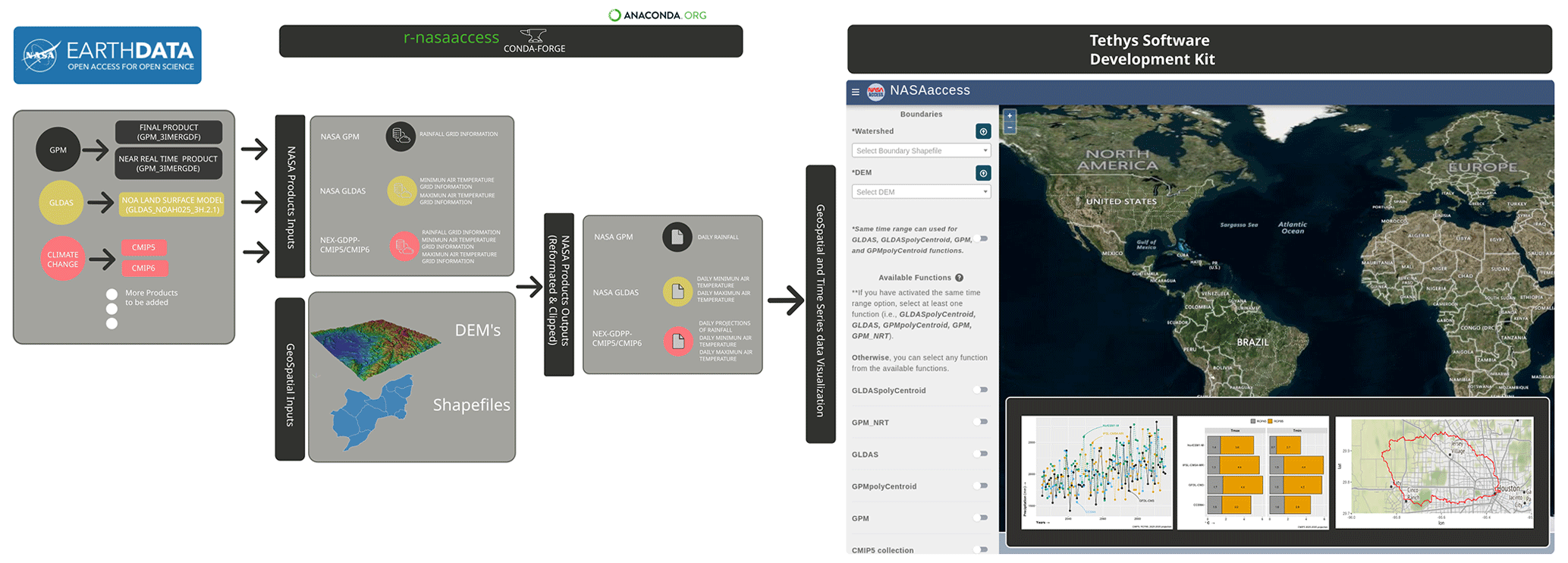
Figure 2 NASAaccess Tethys application flow chart. Map created and drafted using © Microsoft Bing Maps Platform API.

In summary, the NASAaccess Tethys application gives time series and spatial mapping visualization features for all the functions available. Moreover, the user of the NASAaccess Tethys application receives the requested data formatted and ready to be ingested into other modeling frameworks such as the VIC (Liang et al., 1994), DHSVM (Wigmosta et al., 1994), RHESSys model (Tague and Band, 2004), and SWAT (Arnold and Fohrer, 2005) hydrological modeling frameworks. Another feature that the NASAaccess Tethys application supports is the ability to visualize and inspect different datasets processed by different functions at a specific watershed during one or different time periods in one job. This feature is useful when the user is interested in studying the impacts of climate change or any other hydrological regime changes.

2.4 NASAaccess installation steps

2.4.1 R software

On a local machine, the user should have installed the following programs and set up a user account. The list below gives a summary of what is needed to be done prior to working with NASAaccess software on any local machine.

1. Installing R software (The R Project for Statistical Computing, https://www.r-project.org/, last access: 6 October 2023)

2. Installing Rstudio software (Rstudio, https://posit.co/, last access: 6 October 2023) (optional)

3. The NASAaccess R package needs user registration access with Earthdata (NASA Earthdata, https://www.earthdata.nasa.gov/, last access: 6 October 2023). Users should set up a registration account(s) with Earthdata login and authorize NASA GES DISC data access. Please refer to GES DISC data access (https://disc.gsfc.nasa.gov/data-access, last access: 6 October 2023) for further details.

4. After registration with Earthdata NASAaccess software package users should create a reference file (“.netrc”) with Earthdata credentials stored in it to streamline the retrieval access to NASA servers.

   • –

     Creating the .netrc file at the user machine Home directory and storing the user NASA GES DISC logging information in it is needed to execute the NASAaccess package commands. Accessing data at NASA servers is further explained at Earthdata Wiki https://wiki.earthdata.nasa.gov/display/EL/How+To+Access+Data+With+cURL+And+Wget (last access: 6 October 2023).

   • –

     For Windows users, the NASA GES DISC logging information should be saved in a “_netrc” file besides the .netrc file explained above.

5. Install the “curl” software. Since Mac users have curl as part of the macOS build, Windows users should make sure that their local machines' build have curl installed properly.

6. Check whether you can run curl from your command prompt. Type curl --help, and you should see the help pages for the curl program once everything is defined correctly.

7. Within the Rstudio or R terminal run, the following commands install NASAaccess.

       library(devtools)
       install_github("nasa/NASAaccess",
       build_vignettes = TRUE)
       library(NASAaccess)

2.4.2 conda environment

Like the R software, the NASAaccess conda package (r-nasaaccess) needs user registration access with Earthdata (NASA Earthdata, https://www.earthdata.nasa.gov/, last access: 6 October 2023) and to store those credentials in the .netrc reference file as well as create a .urs_cookies file. The .urs_cookies file will be used to persist sessions across individual curl calls, making it more efficient. If the user has successfully prepared the needed steps to run the NASAaccess R package (i.e., creating registration access and storing it in a local machine), then there is no need to duplicate these steps here again. Installing r-nasaaccess in a conda environment allows users to have packages in different programming languages due to the language interoperability of the conda environment. To install the NASAaccess package in Python (r-nasaaccess), run the following syntax in a Python terminal.

conda install -c conda-forge r-nasaaccess

In the Appendix, we give documentation on r-nasaaccess conda configuration and installation steps.

2.4.3 Tethys

The Tethys Platform framework can be installed in a production or development environment. The difference between a production and development installation is that the development server is not efficient or capable of handling the traffic a production website receives, so a combination of the NGINX (https://www.nginx.com/, last access: 6 October 2023) and Daphne (https://github.com/django/daphne, last access: 6 October 2023) servers is used for production installations. In addition, when changes are made to a production installation, such as installing new apps or changing settings, the Daphne server must be restarted manually to load them. It does not restart automatically like the development server. Usually, the development installation is used for app development or local use. The Tethys Platform framework installation process in a development environment is as follows.

1. Create a new conda environment and install Tethys Platform by running the following command.

   conda create -n tethys -c tethysplatform
   -c conda-forge tethys-platform

2. Activate the Tethys conda environment.

   conda activate tethys

3. Generate a portal_config.yml file containing custom configurations such as the database and other local settings by running the following command.

   tethys gen portal_config

4. Tethys Platform requires a PostgreSQL database server. There are several options for setting up a database server: local, docker, or dedicated. Tethys Platform can also be used to create a local server that creates and migrates the tables associated with the Tethys Platform framework by running the following.

   tethys db configure

5. Finally, start the Tethys development server.

   tethys manage start

Installation in a production environment can be a manual installation (performing all the production configuration steps manually) or a docker deployment. The steps for manual and docker installation can be found in the Tethys Platform documentation (http://docs.tethysplatform.org/en/stable/, last access: 6 October 2023). Installation of GeoServer is necessary to use the NASAaccess Tethys application. The GeoServer software can be downloaded and installed on your local machine from https://geoserver.org (last access: 6 October 2023) or using Tethys Platform, which allows users to pull and run a GeoServer container. The following commands can be used to install GeoServer through Tethys Platform: when prompted for a settings value, press Enter to keep the default values.

tethys docker init -c geoserver
tethys docker start -c geoserver

If GeoServer was installed from the source, start GeoServer by changing into the geoserver directory or bin and executing the startup.sh script with the following commands.

cd geoserver/bin
sh startup.sh

Then, in a web browser, navigate to http://localhost:8080/geoserver to ensure that GeoServer has been installed successfully. After successful installation of Tethys Platform and the GeoServer software on your work environment, clone the repository of the NASAaccess application available in GitHub. Next, install the application in Tethys Platform. Once the installation has started, the user will be prompted to select a spatially persistent service and the custom settings related to the application. Finally, start the Tethys development server after the installation has finished. Figure 3 depicts the home window of the NASAaccess Tethys web application. The following commands and steps summarize the process of NASAaccess application installation.

1. git clone (https://github.com/imohamme/tethys_nasaaccess.git)

2. tethys install -d

3. Select the GeoSpatial persistent service (in this case, the installed GeoServer).

4. Enter the value for the custom settings of the NASAaccess application.

   • a.

     data path: custom setting referring to the path of the data directory for download

   • b.

     nasaaccess_R: custom setting referring to the Rbin path

   • c.

     nasaacess_script: custom setting referring to the nasaaccess R script containing the logic for data download using the r-nasaaccess conda package

   • d.

     GeoServer workspace: custom setting referring to the GeoServer workspace name associated with the NASAaccess application

   • e.

     GeoServer uniform resource identifier (URI): custom setting referring to the GeoServer workspace URI associated with the NASAaccess application

   • f.

     GeoServer user: custom setting referring to the GeoServer admin user

   • g.

     GeoServer password: custom setting referring to the password related to the user of the geoserver user setting

5. Then, start Tethys.

   tethys manage start

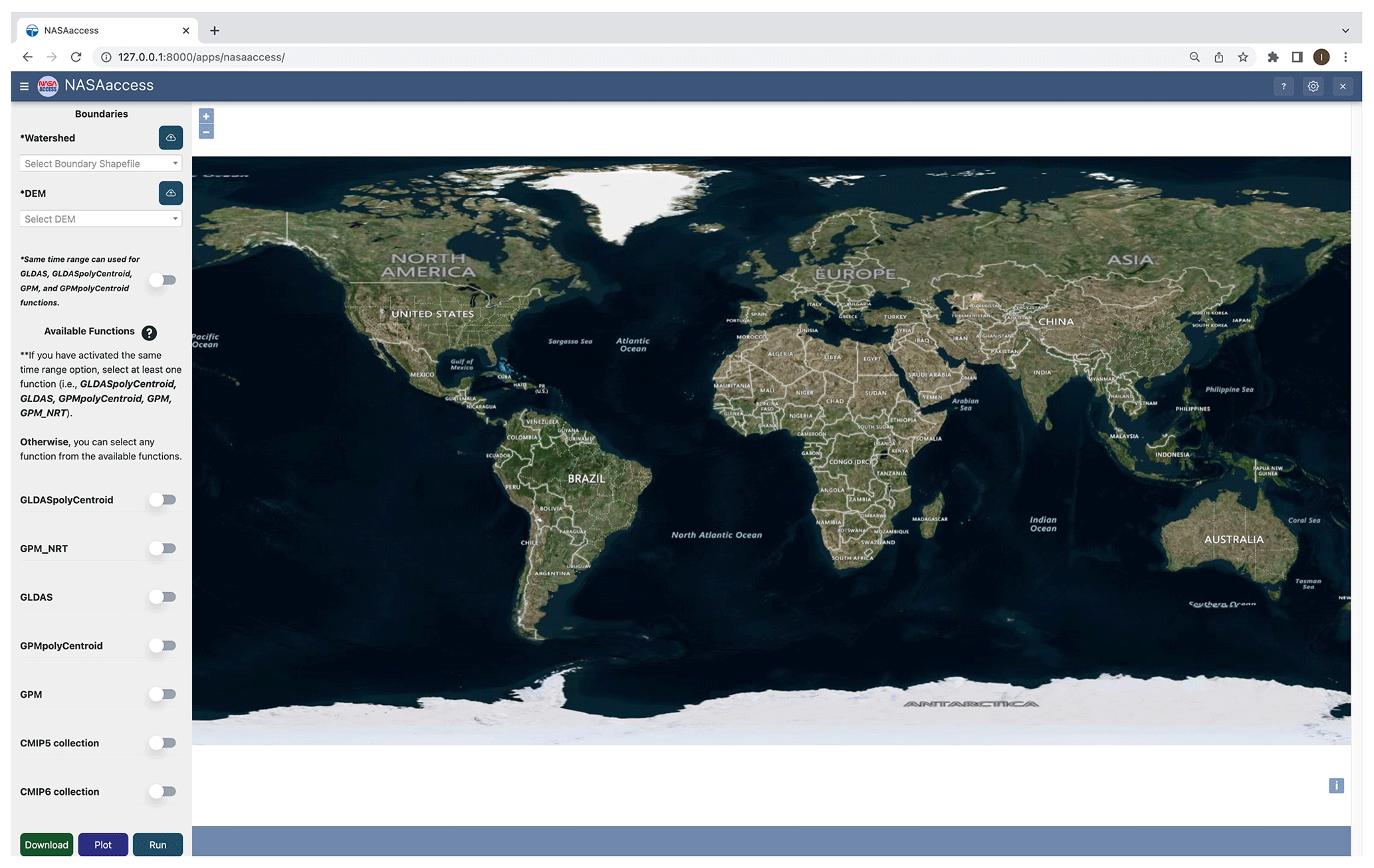
Figure 3 NASAaccess Tethys application home window. Map created and drafted using © Microsoft Bing Maps Platform API.

A detailed installation manual is available in the GitHub repository of the NASAaccess Tethys application (Bustamante and Mohammed, 2023).

3 NASAaccess implementation

3.1 GPM examples with R and conda

The NASAaccess package has multiple functions such as GPM_ NRT, GPMpolyCentroid, and GPMswat that download, extract, and reformat rainfall remote-sensing data of Integrated Multi-satellitE Retrievals for GPM (IMERG) from NASA servers (IMERG, https://gpm.nasa.gov/data/imerg, last access: 6 October 2023) for grids within a specified watershed shapefile. The difference between the GPM_NRT and GPMswat functions is the latency period. The GPMswat function retrieves the IMERG Final Run data which are intended for research-quality global multi-satellite precipitation estimates with quasi-Lagrangian time interpolation, gauge data, and climatological adjustment. On the other hand, the GPM_NRT function retrieves the IMERG near-real-time low-latency gridded global multi-satellite precipitation estimates. Further explanations of the GPM_NRT, GPMpolyCentroid, and GPMswat functions are listed in the NASAaccess documentation part of the Appendix.

Let us explore the GPMpolyCentroid and GPMswat functions' basic use.

Look at an example watershed that we want to examine near Houston, Texas, in the R software platform.

library(ggmap)
#> Loading required package: ggplot2
#> Google's Terms of Service:
https://cloud.google.com/maps-platform/terms/.
#> Please cite ggmap if you use it! See citation("ggmap") for
details.
library(raster)
#> Loading required package: sp
library(ggplot2)
library(rgdal)
#> Please note that rgdal will be retired by the end of 2023,
#> plan transition to sf/stars/terra functions using GDAL and
PROJ
#> at your earliest convenience.
#>
#> rgdal: version: 1.5-30, (SVN revision 1171)
#> Geospatial Data Abstraction Library extensions to R
successfully loaded
#> Loaded GDAL runtime: GDAL 3.4.2, released 2022/03/08
#> Path to GDAL shared files:
/Users/imohamme/Library/R/x86_64/4.1/library/rgdal/gdal
#> GDAL binary built with GEOS: FALSE
#> Loaded PROJ runtime: Rel. 8.2.1, January 1st, 2022,
[PJ_VERSION: 821]
#> Path to PROJ shared files:
/Users/imohamme/Library/R/x86_64/4.1/library/rgdal/proj
#> PROJ CDN enabled: FALSE
#> Linking to sp version:1.4-6
#> To mute warnings of possible GDAL/OSR exportToProj4()
degradation,
#> use options("rgdal_show_exportToProj4_ warnings"="none")
before loading sp or rgdal.
#Reading input data
dem_path <- system.file("extdata",
                        "DEM_TX.tif",
                        package = "NASAaccess")
shape_path <- system.file("extdata",
                          "basin.shp",
                          package = "NASAaccess")
dem <- raster(dem_path)
shape <- readOGR(shape_path)
#> OGR data source with driver: ESRI Shapefile
#> Source:
"/private/var/folders/8t/45w1tdfs1vj3dy1tchbw3pmrhr_gxz/T/
Rtmp1IbSo3/temp_libpath3ee86d57d8b5/NASAaccess/extdata/basin.shp",
layer: "basin"
#> with 1 features
#> It has 4 fields
#> Integer64 fields read as strings:  OBJECTID disID
shape.df <- ggplot2:: fortify(shape)
#> Regions defined for each Polygons
#plot the watershed data
myMap <- get_stamenmap(bbox = c(left = -96,
                                bottom = 29.7,
                                right = -95.2,
                                top = 30),
                                            maptype = "terrain",
                                            crop = TRUE,
                                             zoom = 10)
#> Source : http://tile.stamen.com/terrain/10/238/422.png
#> Source : http://tile.stamen.com/terrain/10/239/422.png
#> Source : http://tile.stamen.com/terrain/10/240/422.png
#> Source : http://tile.stamen.com/terrain/10/241/422.png
#> Source : http://tile.stamen.com/terrain/10/238/423.png
#> Source : http://tile.stamen.com/terrain/10/239/423.png
#> Source : http://tile.stamen.com/terrain/10/240/423.png
#> Source : http://tile.stamen.com/terrain/10/241/423.png
 ggmap(myMap) +
   geom_polygon(data = shape.df,
                aes(x = long, y = lat, group = group),
               fill = NA, size = 0.5, color = 'red')

Figure 4 depicts the geographic layout of the White Oak Bayou watershed example above. The White Oak Bayou is a tributary for the Buffalo Bayou River (Harris County, Texas). To use the NASAaccess library, we also need a digital elevation model (DEM) raster layer. The following is an example of the White Oak Bayou watershed DEM and a closer look at the watershed study example.

# create a plot of our DEM raster along with watershed
library(ggplot2)
library(raster)
library(rgdal)
library(tidyr)
library(cowplot)
library(ggspatial)
dem.df <- as.data.frame(dem,xy=TRUE)%>%drop_na()
ggplot()+
  geom_raster(data=dem.df,aes(x = x,y = y,fill = DEM_TX)) +
  scale_fill_gradientn(name='Elevation (m)', colours =
  terrain.colors(1000))+
  geom_polygon(data = shape.df,aes(x = long, y = lat, group = group),
               fill = NA, linewidth = 0.5, color = 'black')+
  labs(x='Longitude',y='Latitude')+
  cowplot::theme_cowplot()+
  annotation_north_arrow(location = 'tr', which_north = 'true',
  pad_x = unit(0.3, 'in'), pad_y = unit(0.4, 'in'), style =
north_arrow_fancy_orienteering(text_size = 8), height =
unit(0.75, "cm"),
width = unit(0.75, "cm")) +
  annotation_scale(plot_unit='km',location = 'tr', width_hint = 0.3,
pad_y = unit(0.2, 'in'), pad_x = unit(0.2,
'in'), line_width = 0.8)+
  theme(plot.background = element_rect(color = 1,linewidth = 1),
        plot.margin=margin(t = 10, r = 15, b = 10, l = 10,
        unit = "pt"))

Figure 5 gives the White Oak Bayou watershed DEM with an elevation range from 0 to 50 m above sea level. After examining the study watershed and the digital elevation model for it, we can then examine the GPMswat function.

library(NASAaccess)
GPMswat(Dir = "./GPMswat/",
                  watershed = shape_path,
                  DEM = dem_path,
                  start = "2020-08-1",
                  end = "2020-08-3")

The GPMswat function generated data files and a rainfall station file and stored them in the specified Dir examining the rainfall station file generated by GPMswat.

GPMswat.precipitationMaster <- system.file('extdata/GPMswat',
                                        'precipitationMaster.txt',
                                         package = 'NASAaccess')

#Reading textttGPMswat header file
GPMswat.table<-read.csv(GPMswat.precipitationMaster)
head(GPMswat.table)
#>        ID                 NAME      LAT      LONG ELEVATION
#> 1 2160842 precipitation2160842 29.93337 -95.82337  50.16166
#> 2 2160843 precipitation2160843 29.93337 -95.72340  46.68206
#> 3 2160844 precipitation2160844 29.93337 -95.62343  39.72196
#> 4 2160845 precipitation2160845 29.93337 -95.52346  35.58193
#> 5 2164442 precipitation2164442 29.83343 -95.82337  48.02116
#> 6 2164443 precipitation2164443 29.83343 -95.72340  40.47534
dim(GPMswat.table)
#> [1] 11  5

The GPMswat function generated an ASCII table for each available grid located within the study watershed. There are 11 grids within the study watershed, and that means 11 tables have been generated. The GPMswat function also generated the rainfall station file input shown above, GPMswat.table (table with columns ID, File NAME, LAT, LONG, and ELEVATION), for those selected grids that fall within the specified watershed. Now, let us see the locations of these generated grid points.

ggplot() +
  geom_polygon(data = shape.df,
          aes(x = long, y = lat, group = group),
          fill = NA,
          colour = 'black') +
   geom_point(data=GPMswat.table,
              aes(x=LONG,
                  y=LAT,
                  fill=ELEVATION),
              shape=21,
              size = 4) +
   scale_fill_gradientn(name='Elevation (m)', colours =
   terrain.colors(7)) +
   labs(x='Longitude',y='Latitude')+
   theme(plot.background = element_rect(color = 1,linewidth = 1),
         plot.margin=margin(t = 10, r = 15, b = 10, l = 10,
         unit = "pt"))

We note here that GPMswat has given us all the GPM data grids that fall within the boundaries of the White Oak Bayou study watershed (Fig. 6). The time series rainfall data stored in the data tables (i.e., 11 tables) can also be viewed by looking at the reformatted data from the first grid point as listed in the rainfall station file generated by GPMswat.

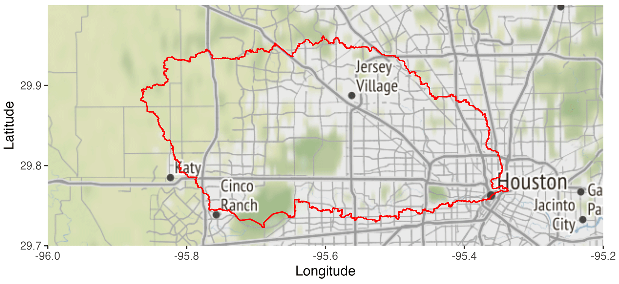
Figure 4 The geographic layout of the White Oak Bayou watershed. The White Oak Bayou is a tributary for the Buffalo Bayou River (Harris County, Texas). Map created and drafted using R: A language and environment for statistical computing version 4.2.2: https://www.R-project.org/ (last access: 6 October 2023) (Vienna, Austria). The map layout was plotted using the EPSG Geodetic Parameter Dataset 4326 projection (https://epsg.io/4326, last access: 6 October 2023).

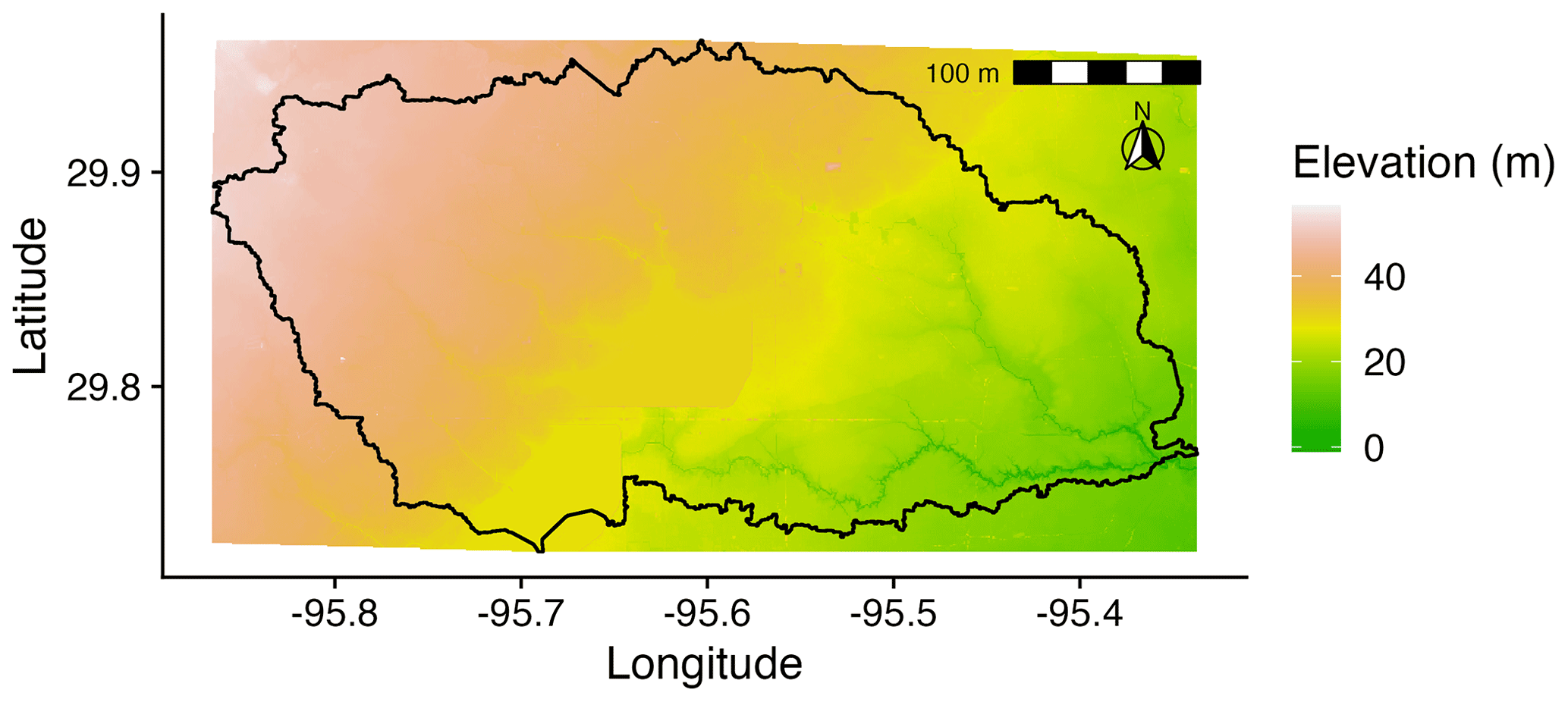
Figure 5 The White Oak Bayou watershed with a digital elevation model. The White Oak Bayou is a tributary for the Buffalo Bayou River (Harris County, Texas). Map created and drafted using R: A language and environment for statistical computing version 4.2.2: https://www.R-project.org/ (last access: 6 October 2023) (Vienna, Austria). The map layout was plotted using the EPSG Geodetic Parameter Dataset 4326 projection (https://epsg.io/4326, last access: 6 October 2023).

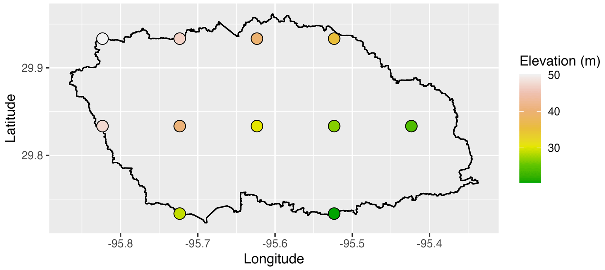
Figure 6 The geographic layout of the White Oak Bayou watershed with the IMERG dataset (GPM Level 3 IMERG Final Daily 0.1 × 0.1^∘, GPM_3IMERGDF) derived from the half-hourly GPM_3IMERGHH data product grids obtained by the GPMswat function of the NASAaccess package that fall within the watershed boundaries. The White Oak Bayou is a tributary for the Buffalo Bayou River (Harris County, Texas). Map created and drafted using R: A language and environment for statistical computing version 4.2.2: https://www.R-project.org/ (last access: 6 October 2023) (Vienna, Austria). The map layout was plotted using the EPSG Geodetic Parameter Dataset 4326 projection (https://epsg.io/4326, last access: 6 October 2023).

GPMswat.point.data <- system.file ('extdata/GPMswat',
                             'precipitation2160842.txt',
                             package = 'NASAaccess')
#Reading data records
read.csv (GPMswat.point.data)
#>     X20200801
#> 1 32.22795868
#> 2  1.80884695
#> 3  0.07029478

GPMswat has generated ready-formatted ASCII tables that can be ingested easily into any hydrological model of choice.

Now, let us examine GPMpolyCentroid.

GPMpolyCentroid(Dir = "./GPMpolyCentroid/",
                  watershed = shape_path,
                  DEM = dem_path,
                  start = "2019-08-1",
                  end = "2019-08-3")

Examine the rainfall station file generated by GPMpolyCentroid.

GPMpolyCentroid.precipitationMaster <- system.file
                             ('extdata/GPMpolyCentroid',
                             'precipitationMaster.txt',
                              package = 'NASAaccess')
GPMpolyCentroid.precipitation.table <- read.csv
(GPMpolyCentroid.precipitationMaster)
#plotting
ggplot() +
  geom_polygon(data = shape.df,
                aes(x = long, y = lat, group = group),
                fill = NA,
                colour = 'red') +
   geom_point(data=GPMpolyCentroid.precipitation.table,
              aes(x=LONG,y=LAT)) +
   labs(x='Longitude',y='Latitude')+
   theme(plot.background = element_rect(color = 1,linewidth = 1),
         plot.margin=margin(t = 10, r = 15, b = 10, l = 10,
         unit = "pt"))

We note here that GPMpolyCentroid has given us the GPM data grid that falls within a specified watershed and that assigns to a pseudo rainfall gauge located at the centroid of the watershed weighted-average daily rainfall data (Fig. 7). Let us then examine the precipitation data just obtained by GPMpolyCentroid over the White Oak Bayou study watershed.

GPMpolyCentroid.precipitation.record <-
                   system.file('extdata/GPMpolyCentroid',
                   'precipitation1.txt',
                   package = 'NASAaccess')
GPMpolyCentroid.precipitation.data <-
read.csv(GPMpolyCentroid.precipitation.record)
#since data started on 2019-08-01
days <- seq.Date(from = as.Date('2019-08-01'),
                 length.out =
                 dim(GPMpolyCentroid.precipitation.data)[1],
                 by = 'day')
#plotting the precipitation time series
df <- data.frame(day=days,Precipitation=GPMpolyCentroid.
precipitation.data [,1])
ggplot(data=df, aes(days, Precipitation)) +
  geom_point()+
  geom_line()+
  labs(x='Longitude',y='Latitude')+
  theme(plot.background = element_rect(color = 1,linewidth = 1),
        plot.margin=margin(t = 10, r = 15, b = 10, l = 10,
        unit = "pt"))

The time series plot above gives the rainfall amounts in millimeters at the centroid of the White Oak Bayou watershed from 1 to 3 August 2019 that are shown in Fig. 8. Finally, let us examine the near-real-time precipitation data obtained by GPM_NRT over the White Oak Bayou study watershed. Remember that the minimum latency for GPM_NRT is 1 d.

GPM_NRT(Dir = "./GPM_NRT/",
                  watershed = shape_path,
                  DEM = dem_path,
                  start = "2022-07-1",
                  end = "2022-07-3")

Let us look at the one-point data record. Note that the data start on 1 July 2022 and end on 3 July 2022.

GPM_NRT.point.data <- system.file('extdata/GPM_NRT',
                              'precipitation2160845.txt',
                              package = 'NASAaccess')
#Reading data records
read.csv(GPM_NRT.point.data)
#>   X20220701
#> 1  2.507078
#> 2  1.148573
#> 3  0.000000

The above examples were obtained using R version 4.2.2 (R Development Core Team, 2022). The R software program and all the packages used are available from the CRAN at https://CRAN.R-project.org (last access: 6 October 2023). There are multiple factors such as Internet bandwidth (i.e., the volume of information that can be sent over a connection in a measured amount of time), Internet speed, and study site size that interact in figuring out the time duration of any NASAaccess function execution. To illustrate this further, here is an example of 1-month data record retrieval using the GPM_NRT function over the same study site shown above.

system.time({ GPM_NRT(Dir = "./GPM_NRT_2/",
                       watershed = shape_path,
                       DEM = dem_path,
                       start = "2023-04-01",
                       end = "2023-04-30") })
#Results
#user system elapsed
#30.023 21.869 130.313

The results give “user”, “system”, and “elapsed” times. The user gives the CPU time spent by the current process (i.e., the current R session) in seconds, and the system gives the CPU time spent by the kernel (the operating system) on behalf of the current process in seconds. The elapsed time is the wall clock time taken to execute the GPM_NRT function (i.e., 130.313 s). Upon checking the Internet speed utilized on a (Intel(R) Core(TM) i9-9880H CPU @ 2.30 GHz) machine, this reveals the following.

==== SUMMARY ====
Upload capacity: 17.543 Mbps
Download capacity: 107.578 Mbps
Upload flows: 12
Download flows: 12
Responsiveness: Medium (714 RPM)

The reader is encouraged to visit NASAaccess articles (https://imohamme.github.io/NASAaccess/articles/About.html, last access: 6 October 2023) for detailed package documentation and vignettes, including demonstration on GLDAS, CMIP5, and CMIP6. The above NASAaccess GPM examples can easily be replicated in the conda environment by writing the NASAaccess commands shown above to a separate file (e.g., work.R) and running the separate file by calling the Rscript executable in conda.

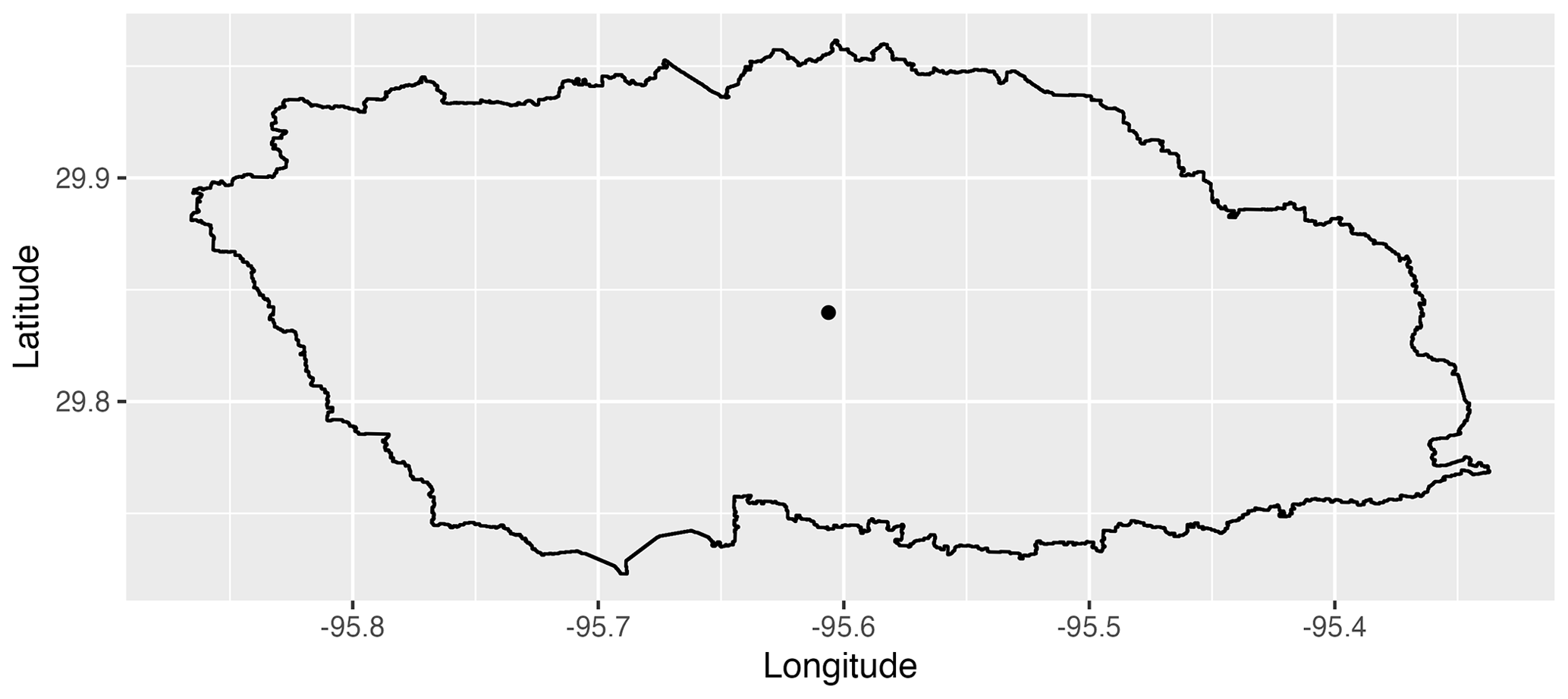
Figure 7 The geographic layout of the White Oak Bayou watershed with a data grid obtained by the GPMpolyCentroid function of the NASAaccess package. The GPMpolyCentroid function assigns to a pseudo rainfall gauge located at the centroid of the watershed weighted-average daily rainfall data from the IMERG dataset (GPM_3IMERGDF) derived from the half-hourly GPM_3IMERGHH data products. The White Oak Bayou is a tributary for the Buffalo Bayou River (Harris County, Texas). Map created and drafted using R: A language and environment for statistical computing version 4.2.2: https://www.R-project.org/ (last access: 6 October 2023) (Vienna, Austria). The map layout was plotted using the EPSG Geodetic Parameter Dataset 4326 projection (https://epsg.io/4326, last access: 6 October 2023).

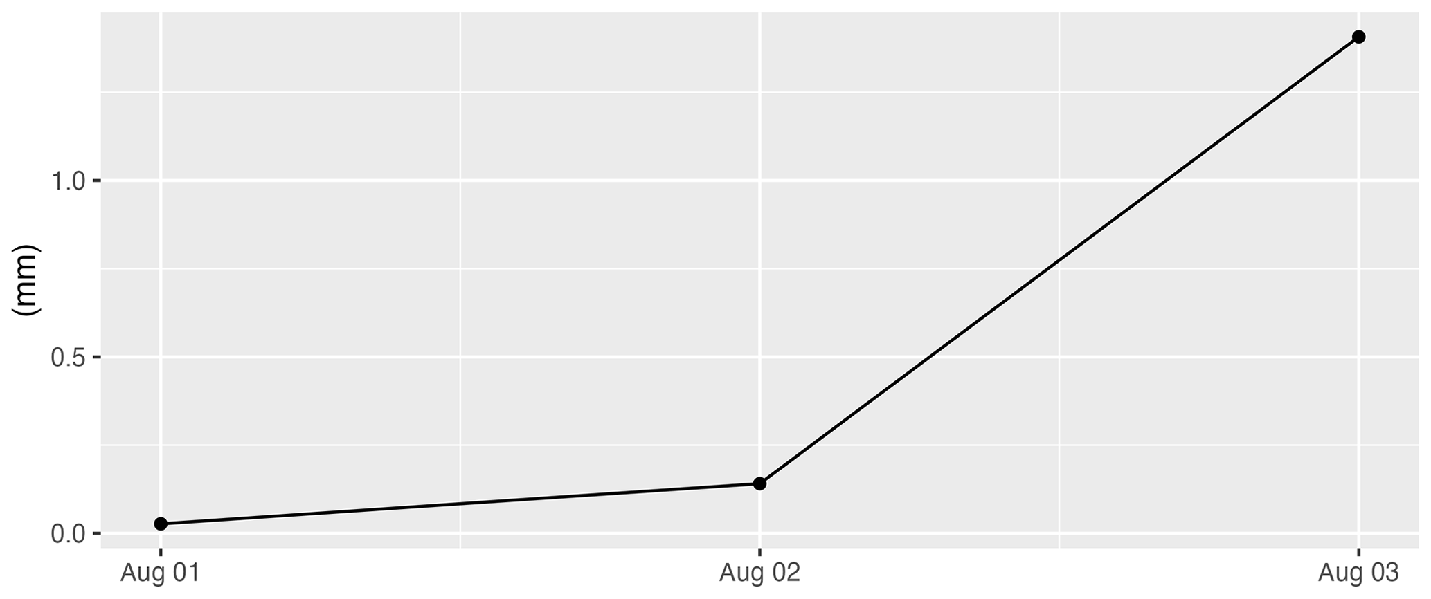
Figure 8 The rainfall amounts in millimeters at the centroid of the White Oak Bayou watershed from 1 to 3 August 2019 as obtained by the GPMpolyCentroid function. The GPMpolyCentroid function assigns to a pseudo rainfall gauge located at the centroid of the watershed weighted-average daily rainfall data from the IMERG dataset (GPM_3IMERGDF) derived from the half-hourly GPM_3IMERGHH data products. The White Oak Bayou is a tributary for the Buffalo Bayou River (Harris County, Texas).

In conda, assuming r-nasaaccess has been installed successfully, this can be done as follows.

Rscript work.R

3.2 NASAaccess Tethys examples

The NASAaccess Tethys application adds visualization features to NASAaccess R and conda packages. Figure 9 depicts rainfall remote-sensing data of GPM IMERG from NASA servers (https://gpm.nasa.gov/data/imerg, last access: 6 October 2023) for grids within the White Oak Bayou watershed from 1 January to 31 December 2020 as processed by the GPMpolyCentroid function part of the NASAaccess Tethys application. The user can inspect individual grid time series data. This is helpful when looking at different datasets such as historical and projected air temperature and precipitation time series data on one grid. In Fig. 10, we present daily diurnal air temperature data processed over the same watershed discussed in Fig. 9 (the White Oak Bayou watershed) during the same period (e.g., January to December 2020). The GLDASpolyCentroid function was selected to visualize and reformat the GLDAS Noah land surface model L4 3-hourly 0.25 × 0.25^∘ V2.1 air temperature dataset (Rodell et al., 2004) in Fig. 10.

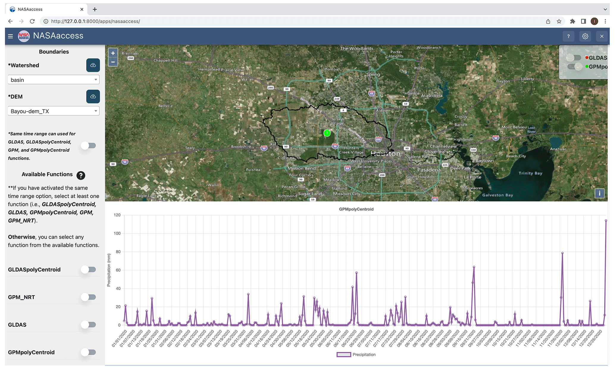
Figure 9 The rainfall amounts in millimeters at the centroid of the White Oak Bayou watershed from 1 January to 31 December 2020 as obtained by the GPMpolyCentroid function and presented by the NASAaccess Tethys application. The GPMpolyCentroid function assigns to a pseudo rainfall gauge located at the centroid of the watershed weighted-average daily rainfall data from the IMERG dataset (GPM_3IMERGDF) derived from the half-hourly GPM_3IMERGHH data products. The White Oak Bayou is a tributary for the Buffalo Bayou River (Harris County, Texas). Map created and drafted using © Microsoft Bing Maps Platform API.

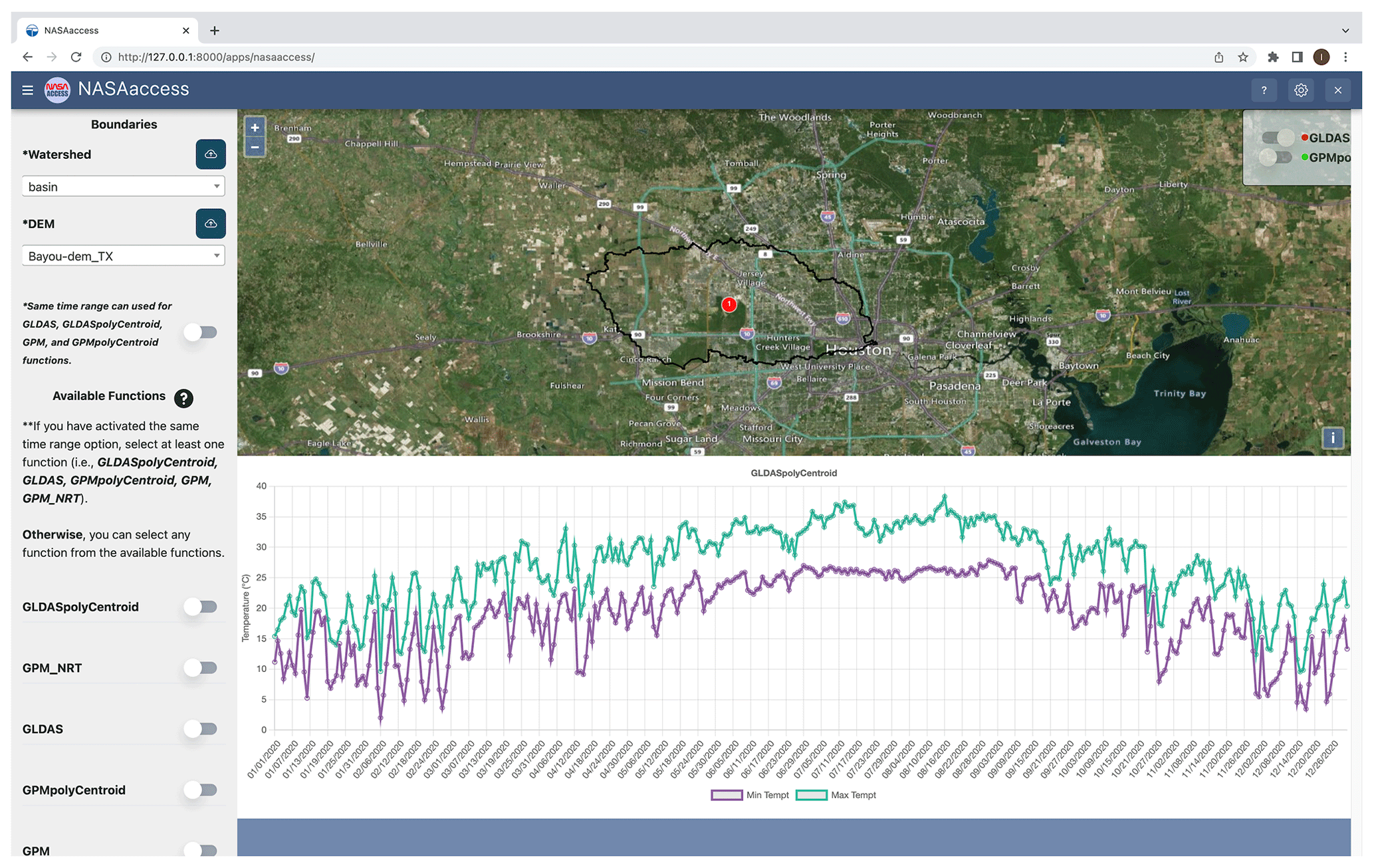
Figure 10 The daily diurnal air temperature (minimum and maximum) in degrees Celsius at the centroid of the White Oak Bayou watershed from 1 January to 31 December 2020 as obtained by the GLDASpolyCentroid function of the NASAaccess Tethys application. The GLDASpolyCentroid function assigns to a pseudo air temperature gauge located at the centroid of the White Oak Bayou watershed weighted-average daily minimum and maximum air temperature data from the GLDAS Noah land surface model L4 3-hourly 0.25 × 0.25^∘ V2.1. The White Oak Bayou is a tributary for the Buffalo Bayou River (Harris County, Texas). Map created and drafted using © Microsoft Bing Maps Platform API.

The NASAaccess Tethys application has visualization features for downscaled climate data that include the CMIP5 and CMIP6 collections. In Fig. 11, we give a downscaled precipitation data scenario during the year 2045 for the La Plata Basin derived from the National Oceanic and Atmospheric Administration (NOAA) Geophysical Fluid Dynamics Laboratory General Circulation Model – GFDL-ESM2M – across the greenhouse gas emission representative concentration pathways (RCPs) (rcp85) using the NEX_GDDP_CMIP5 function. More details on the NEX_GDDP_CMIP6 and NEX_ GDDP_CMIP5 functions and the downscaled models covered are provided in the Appendix B NASAaccess documentation.

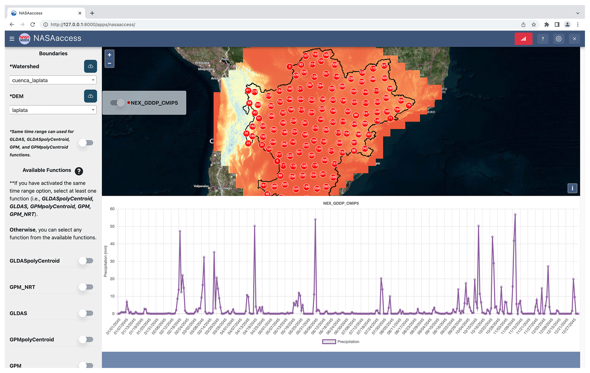
Figure 11 The daily downscaled precipitation in millimeters projected by the GFDL-ESM2M model across the rcp85 greenhouse gas emission at the La Plata Basin from 1 January to 31 December 2045 as obtained by the NEX_GDDP_CMIP5 function of the NASAaccess Tethys application. The NEX_GDDP_CMIP5 generates downscaled daily precipitation and diurnal air temperature data from the NASA CMIP5 downscaled climate change data products. The La Plata Basin depicted with the digital elevation model layer includes areas of southeastern Bolivia, southern and central Brazil, the entire country of Paraguay, most of Uruguay, and northern Argentina. Map created and drafted using © Microsoft Bing Maps Platform API.

4 Discussion

The NASAaccess package presented provides open-source remote-sensing earth observation data access, visualization, and reformatting for an easy-ingestion platform. The biggest advantage we see is the utility of NASAaccess in facilitating the access, processing, and visualization of various remote-sensing earth observation data to scientific and decision-maker audiences. This is in line with the NASA OSSI call for more open-source science work. This NASAaccess work has the potential to increase the remote-sensing earth observation data products' accessibility on various computing platforms to enhance the progress of science in earth observation data access and management. NASAaccess development is in line with international calls for and efforts in open science, scientific information, knowledge, data, and protocol sharing (UNESCO Open Science, https://www.unesco.org/en/open-science, last access: 6 October 2023). We have demonstrated the linkage of the NASAaccess platform in the SWATOnline example (McDonald et al., 2019), where a decision support system for the lower Mekong River Basin has been shown. Another potential application could also be shown in disseminating climate information for developing countries (Dinku et al., 2014, 2018), similar to our demonstration in the Se Kong, Se San, and Sre Pok parts of the lower Mekong (Mohammed et al., 2022). NASAaccess also gives the user an automatic, quick, and accurate way of working with remote-sensing earth observation data using R and conda environments. This presented application would increase awareness, accelerate progress, and facilitate access to remote-sensing earth observation data, tools, and knowledge about our changing environment. Moreover, it helps to assist in addressing major research gaps in climatological and hydrological science, especially in management, interdisciplinary communication, as well as modeling and monitoring. In Table 1, we highlighted some NASA GES DISC tools and services for accessing and visualizing earth observation remote-sensing data. The NASAaccess framework benefits can then be summarized as (1) an open-source tool; (2) modular, which means that the framework could be replicated, customized, and implemented anywhere; (3) seamless earth observation remote-sensing and climate data ingestion into other modeling frameworks – NASAaccess gives the ready-formatted ASCII data required to drive various hydrological models; and (4) lowering the technical barrier to leveraging and visualizing a wide array of satellite-based earth observations.

NASAaccess has been introduced to the SERVIR, a joint initiative of the National Aeronautics and Space Administration (NASA) and United States Agency for International Development (USAID), and leading geospatial organizations in Asia, Africa, and Latin America (https://www.nasa.gov/mission_pages/servir/overview.html, last access: 6 October 2023) and Group of Earth Observation Global Water Sustainability (GEOGloWS, https://www.geoglows.org/, last access: 6 October 2023) research network communities through workshops, seminars, and training events. SERVIR, a United States Agency for International Development (USAID) and NASA collaborative project, has multiple global networks that cover different geographic regions such as the Hindu Kush–Himalaya, lower Mekong, and Amazonia. For instance, in alignment with the U.S. Indo-Pacific Vision to improve the management of natural resources, SERVIR-Mekong launched a series of regional tools and services utilizing publicly available satellite imagery and geospatial technologies to support the lower Mekong region in managing environmental risks by enhancing drought resilience and crop yield security, improving regional land cover monitoring, and supporting better flood forecasting and early warning.

NASAaccess has also been leveraged via the GEOGloWS Tethys portal. GEOGloWS is a voluntary partnership of governments and international organizations. GEOGloWS provides a framework within which these partners can develop new projects and coordinate their strategies and investments. The GEOGloWS working group 2 initiative works on the application of information and communication technologies (ICTs), also known as hydroinformatics, to address the issues related to data analysis, data handling, data management, and data integration methodologies to translate scientific data to knowledge products that are informative, intuitive, understandable, and supportive in the decision-making process. It is important to highlight here that the GEOGloWS Tethys portal system is free, available for use in locations worldwide, and developed from services that allow customization for a variety of derivative applications.

In summary, the approach we implemented lowers the barrier between water resources and remote-sensing web development, as highlighted by Swain et al. (2016). The NASAaccess web-based application has visualization capabilities that make it easy to inspect and analyze various remote-sensing earth observation data products. Examples of applications of the GPM functions within the platform have been shown. NASAaccess has the advantage that remote-sensing data products are easily processed and analyzed within multiple computational frameworks such as conda and R. This feature allows users to save time for more in-depth analysis. For instance, modelers who are interested in forcing hydrological models with GPM precipitation data will find it very easy to obtain and process GPM data products using NASAaccess. In further updates of the platform, more earth observation remote-sensing products (e.g., ICESat-2 products https://icesat-2.gsfc.nasa.gov/science/data-products, last access: 6 October 2023) will be implemented to widen the NASAaccess utility application areas. Moreover, accessing remote-sensing products that characterize water storage changes in lakes, reservoirs, and large river channels obtained through the Surface Water and Ocean Topography satellite mission (SWOT, https://swot.jpl.nasa.gov/, last access: 6 October 2023) will be included.

5 Conclusions

NASAaccess is an open-source software package and web-based environmental modeling application for earth observation data accessing, reformatting, and presenting quantitative data products. NASAaccess gives ready-formatted ASCII data required to drive various hydrological models. NASAaccess is a response to the OSSI and lowers the technical barrier to leveraging and visualizing a wide array of satellite-based earth observations.

Appendix A: NASAaccess conda installation documentation

The r-nasaaccess conda package needs user registration with Earthdata (https://www.earthdata.nasa.gov/, last access: 6 October 2023). As we discussed earlier in the NASAaccess installation steps, users should create a reference file (“.netrc”) with Earthdata credentials stored in it to streamline the retrieval access to NASA servers. In conda, users should make sure to update the conda initial script with the .netrc file location. Here is the information from a local-machine r-nasaaccess installation.

conda info
        active environment : None
        user config file : /Users/imohamme/.condarc
        populated config files : /Users/imohamme/.condarc
        conda version : 23.1.0
        conda-build version : not installed
        Python version : 3.7.12.final.0
        virtual packages : __archspec=1=x86_64
                      __osx=10.16=0
                      __unix=0=0
        base environment : /Users/imohamme/opt/miniconda3  (writable)
        conda av data dir : /Users/imohamme/opt/miniconda3/etc/conda
        conda av metadata url : None
        channel URLs : https://conda.anaconda.org/conda-forge/osx-64
                       https://conda.anaconda.org/conda-forge/noarch
                       https://conda.anaconda.org/bioconda/osx-64
                       https://conda.anaconda.org/bioconda/noarch
                       https://conda.anaconda.org/r/osx-64
                       https://conda.anaconda.org/r/noarch
                       https://repo.anaconda.com/pkgs/main/osx-64
                       https://repo.anaconda.com/pkgs/main/noarch
                       https://repo.anaconda.com/pkgs/r/osx-64
                       https://repo.anaconda.com/pkgs/r/noarch
       package cache : /Users/imohamme/opt/miniconda3/pkgs
                     /Users/imohamme/.conda/pkgs
       envs directories : /Users/imohamme/opt/miniconda3/envs
                      /Users/imohamme/.conda/envs
                platform : osx-64
                user-agent : conda/23.1.0 requests/2.28.2
                CPython/3.7.12 Darwin/21.6.0 OSX/10.16
                UID:GID : 562380735:1286109195
                netrc file : /Users/imohamme/.netrc
                offline mode : False

Installing the r-nasaaccess conda package is done by the following.

conda install -c conda-forge r-nasaaccess

Appendix B: NASAaccess documentation

The NASAaccess documentation contains the following functions.

• NEX_GDDP_CMIP6. The NEX-GDDP-CMIP6 dataset is comprised of downscaled climate scenarios for the globe that are derived from the general circulation model (GCM) runs conducted under CMIP6 (Eyring et al., 2016) and across the four “Tier 1” greenhouse gas emission scenarios known as shared socioeconomic pathways (SSPs) (O'Neill et al., 2016; Meinshausen et al., 2020). The CMIP6 GCM runs were developed in support of the Sixth Assessment Report of the Intergovernmental Panel on Climate Change (IPCC AR6). This dataset includes downscaled projections from the 35 models and scenarios for which daily scenarios were produced and distributed under CMIP6. The bias-correction spatial disaggregation (BCSD) method used in generating the NEX-GDDP-CMIP6 dataset is a statistical downscaling algorithm specifically developed to address the current limitations of the global GCM outputs (Wood et al., 2002, 2004; Maurer and Hidalgo, 2008; Thrasher et al., 2012). The NEX-GDDP-CMIP6 climate projections are downscaled at a spatial resolution of 0.25^∘ × 0.25 ^∘ (approximately 25 km × 25 km). NEX_GDDP_CMIP6 downscales the NEX-GDDP data to grid points of 0.1^∘ × 0.1^∘ following nearest-point methods described by Mohammed et al. (2018). The NEX_GDDP_CMIP6 syntax is as follows.

  $$\begin{array}{}\text{(B1)}& \begin{array}{rl}& \mathtt{\text{NEX\_GDDP\_CMIP6(Dir = "./INPUT/", watershed = }}\\ & \mathtt{\text{"watershed.shp", DEM = "watershed\_dem.tif",}}\\ & \mathtt{\text{start = "2060-12-1", end = "2060-12-3",}}\\ & \mathtt{\text{model = "MIROC6" , type = "pr" , slice = "ssp245")}}\end{array}\end{array}$$

  Arguments

  Dir

  A directory name to store gridded climate data and station files

  watershed

  A study watershed shapefile spatially describing polygon(s) in a geographic projection sp::CRS(“+ proj = longlat + datum = WGS84”)

  DEM

  A study watershed digital elevation model raster in a geographic projection sp::CRS(“+ proj = longlat + datum = WGS84”)

  start

  This is the beginning date for gridded climate data and should be equal to or greater than 1 January 2006 for the rcp45 or rcp85 RCP climate scenarios. Also, the start should be equal to or greater than 1 January 1950, and the end should be equal to or less than 31 December 2005 for the “historical” GCM retrospective climate data.

  end

  Ending date for gridded climate data

  model

  This is climate modeling center and name from the World Climate Research Programme (WCRP) global climate projections through CMIP6 (e.g., MIROC6, which is the sixth version of the Model for Interdisciplinary Research on Climate – MIROC).

  type

  This is a flux data type. Its value can be “pr” for precipitation or “tas” for air temperature.

  slice

  This is a scenario from the SSPs. Its value can be “ssp126”, “ssp245”, “ssp370”, “ssp585”, or “historical”.

• NEX_GDDP_CMIP5. The NEX_GDDP_CMIP5 function downloads and processes climate change data of rainfall and air temperature from NEX-GDDP Goddard Space Flight Center servers (https://www.nccs.nasa.gov/services/data-collections/land-based-products/nex-gddp, last access: 6 October 2023), extracts data from grids within a specified watershed shapefile, and then generates tables in a format that any hydrological model requires for rainfall or air temperature data input. The NEX_GDDP_CMIP5 function also generates the climate station file input (files with columns ID, File NAME, LAT, LONG, and ELEVATION) for those selected climatological grids that fall within the specified watershed. The NEX-GDDP dataset is comprised of downscaled climate scenarios for the globe that are derived from the GCM runs conducted under CMIP5 (Taylor et al., 2012) and across two of the four greenhouse gas emission scenarios, rcp45 and rcp85, known as RCPs (Meinshausen et al., 2011). The CMIP5 GCM runs were developed in support of the Fifth Assessment Report of the Intergovernmental Panel on Climate Change (IPCC AR5). This dataset includes downscaled projections from the 21 models and scenarios for which daily scenarios were produced and distributed under CMIP5. The BCSD method used in generating the NEX-GDDP dataset is a statistical downscaling algorithm specifically developed to address the current limitations of the global GCM outputs (Wood et al., 2002, 2004; Maurer and Hidalgo, 2008; Thrasher et al., 2012). The NEX-GDDP climate projections are downscaled at a spatial resolution of 0.25^∘ × 0.25^∘ (approximately 25 km × 25 km). NEX_GDDP_ CMIP5 downscales the NEX-GDDP data to grid points of 0.1 ^∘ × 0.1^∘ following the nearest-point methods described by Mohammed et al. (2018). The NEX_GDDP_CMIP5 syntax is as follows.

  $$\begin{array}{}\text{(B2)}& \begin{array}{rl}& \mathtt{\text{NEX\_GDDP\_CMIP5(Dir = "./INPUT/",}}\\ & \mathtt{\text{watershed = "watershed.shp",}}\\ & \mathtt{\text{DEM = "watershed\_dem.tif", start = "2060-12-1",}}\\ & \mathtt{\text{end = "2060-12-3", model = "IPSL-CM5A-MR",}}\\ & \mathtt{\text{type ="pr" , slice ="rcp85")}}\end{array}\end{array}$$

  Arguments

  Dir

  A directory name to store gridded climate data and station files

  watershed

  A study watershed shapefile spatially describing polygon(s) in a geographic projection sp::CRS(“+ proj = longlat + datum = WGS84”)

  DEM

  A study watershed digital elevation model raster in a geographic projection sp::CRS(“+ proj = longlat + datum = WGS84”)

  start

  This is the beginning date for gridded climate data and should be equal to or greater than 1 January 2006 for the rcp45 or rcp85 RCP climate scenarios. Also, the start should be equal to or greater than 1 January 1950, and the end should be equal to or less than 31 December 2005 for the historical GCM retrospective climate data.

  end

  Ending date for gridded climate data

  model

  This is a climate modeling center and name from the WCRP global climate projections through CMIP5 (e.g., IPSL-CM5A-MR, which is the Institut Pierre-Simon Laplace CM5A-MR model).

  type

  This is a flux data type. Its value can be “pr” for precipitation or “tas” for air temperature.

  slice

  This is a scenario from the RCPs. Its value can be rcp45, rcp85, or “historical”.

• GPM_NRT. The GPM_NRT function downloads and processes rainfall remote-sensing data of the Integrated Multi-satellitE Retrievals for GPM (IMERG) from NASA GSFC servers, extracts data from grids within a specified watershed shapefile, and then generates tables in a format that any hydrological model requires for rainfall data input. The GPM_NRT function also generates the rainfall station file input (files with columns ID, File NAME, LAT, LONG, and ELEVATION) for those selected grids that fall within the specified watershed. The minimum latency for the GPM_NRT function is 1 d. The GPM_NRT function accesses the NASA Goddard Space Flight Center server address for IMERG remote-sensing data products at https://gpm1.gesdisc.eosdis.nasa.gov/data/GPM_L3/GPM_3IMERGDE.06/ (last access: 6 October 2023). The IMERG dataset used by GPM_NRT is the GPM Level 3 IMERG Early Daily 0.1 × 0.1^∘ (GPM_3IMERGDE) derived from the half-hourly GPM_3IMERGHHE. The derived result represents the final estimate of the daily accumulated precipitation. The IMERG dataset is produced at the NASA GES DISC by simply summing the valid precipitation retrievals for the day in GPM_3IMERGHHE and giving the result in millimeters. The GPM_NRT function uses a variable name (“precipitationCal”) for rainfall in IMERG data products. The IMERG data products are available from 1 June 2000 to the present. The GPM_NRT function outputs table and gridded data files matching the grid point resolution of IMERG data products (i.e., a resolution of 0.1^∘). The GPM_NRT syntax is as follows.

  $$\begin{array}{}\text{(B3)}& \begin{array}{rl}& \mathtt{\text{GPM\_NRT(Dir = "./INPUT/",}}\\ & \mathtt{\text{watershed = "watershed.shp", }}\\ & \mathtt{\text{DEM = "watershed\_dem.tif", start = "2015-12-1",}}\\ & \mathtt{\text{end = "2015-12-3")}}\end{array}\end{array}$$

  Arguments

  Dir

  A directory name to store gridded rainfall and rain station files

  watershed

  A study watershed shapefile spatially describing polygon(s) in a geographic projection sp::CRS(“+ proj = longlat + datum = WGS84”)

  DEM

  A study watershed digital elevation model raster in a geographic projection sp::CRS(“+ proj = longlat + datum = WGS84”)

  start

  This is the beginning date for gridded rainfall data, and it should be equal to or greater than 1 June 2000.

  end

  Ending date for gridded rainfall data

• GPMpolyCentroid. The GPMpolyCentroid function downloads and processes rainfall remote-sensing data of IMERG from NASA GSFC servers, extracts data from grids falling within a specified subbasin(s) watershed shapefile, and assigns to a pseudo rainfall gauge located at the centroid of the subbasin(s) watershed weighted-average daily rainfall data. The function generates rainfall tables in a format that any rainfall-runoff hydrological model requires for rainfall data input. The function also generates the rainfall station file summary input (files with columns ID, File NAME, LAT, LONG, and ELEVATION) for those pseudo grids that correspond to the centroids of the watershed subbasins. The minimum latency for the GPMpolyCentroid function is 3.5 months. The GPMpolyCentroid function accesses the NASA Goddard Space Flight Center server address for IMERG remote-sensing data products at https://gpm1.gesdisc.eosdis.nasa.gov/data/GPM_L3/GPM_3IMERGDF.06/ (last access: 6 October 2023). The IMERG dataset used by the GPMpolyCentroid function is the GPM Level 3 IMERG Final Daily 0.1 × 0.1^∘ (GPM_3IMERGDF) derived from the half-hourly GPM_3IMERGHH. This derived result represents the final estimate of the daily accumulated precipitation. The GPM_3IMERGDF dataset is produced at the NASA GES DISC by simply summing the valid precipitation retrievals for the day in GPM_3IMERGHH and giving the result in millimeters. The GPMpolyCentroid syntax is as follows.

  $$\begin{array}{}\text{(B4)}& \begin{array}{rl}& \mathtt{\text{GPMpolyCentroid(Dir = "./INPUT/",}}\\ & \mathtt{\text{watershed = "watershed.shp",}}\\ & \mathtt{\text{DEM = "watershed\_dem.tif", start = "2015-12-1",}}\\ & \mathtt{\text{end = "2015-12-3")}}\end{array}\end{array}$$

  Arguments

  Dir

  A directory name to store gridded rainfall and rain station files

  watershed

  A study watershed shapefile spatially describing polygon(s) in a geographic projection sp::CRS(“+ proj = longlat + datum = WGS84”)

  DEM

  A study watershed digital elevation model raster in a geographic projection sp::CRS(“+ proj = longlat + datum = WGS84”)

  start

  This is the beginning date for gridded rainfall data, and it should be equal to or greater than 1 March 2000.

  end

  Ending date for gridded rainfall data

• GPMswat. The GPMswat function downloads and processes rainfall remote-sensing data of IMERG from NASA GSFC servers, extracts data from grids within a specified watershed shapefile, and then generates tables in a format that the SWAT (https://swat.tamu.edu/, last access: 6 October 2023) hydrological model requires for rainfall data input. The function also generates the rainfall station file input (files with columns ID, File NAME, LAT, LONG, and ELEVATION) for those selected grids that fall within the specified watershed. The minimum latency for the GPMswat function is 3.5 months. The GPMswat function accesses the NASA Goddard Space Flight Center server address for IMERG remote-sensing data products at https://gpm1.gesdisc.eosdis.nasa.gov/data/GPM_L3/GPM_3IMERGDF.06/ (last access: 6 October 2023). The IMERG dataset used by the GPMswat function is GPM_3IMERGDF derived from the half-hourly GPM_3IMERGHH. This derived result represents the final estimate of the daily accumulated precipitation. The GPM_3IMERGDF dataset is produced by NASA GES DISC. The GPM_3IMERGDF dataset's unit is millimeters. The GPMswat syntax is as follows.

  $$\begin{array}{}\text{(B5)}& \begin{array}{rl}& \mathtt{\text{GPMswat(Dir="./INPUT/",}}\\ & \mathtt{\text{watershed = "watershed.shp",}}\\ & \mathtt{\text{DEM = "watershed\_dem.tif"}},\\ & \mathtt{\text{start = "2015-12-1", end = "2015-12-3")}}\end{array}\end{array}$$

  Arguments

  Dir

  A directory name to store gridded rainfall and rain station files

  watershed

  A study watershed shapefile spatially describing polygon(s) in a geographic projection sp::CRS(“+ proj = longlat + datum = WGS84”)

  DEM

  A study watershed digital elevation model raster in a geographic projection sp::CRS(“+ proj = longlat + datum = WGS84”)

  start

  This is the beginning date for gridded rainfall data, and it should be equal to or greater than 1 March 2000.

  end

  Ending date for gridded rainfall data

• GLDASpolyCentroid. The GLDASpolyCentroid function downloads and processes the remote-sensing data product of GLDAS from NASA Goddard Space Flight Center (GSFC) servers, extracts air temperature data from grids falling within a specified subbasin(s) watershed shapefile, and assigns to a pseudo air temperature gauge located at the centroid of the subbasin(s) watershed weighted-average daily minimum and maximum air temperature data. The GLDASpolyCentroid function generates ASCII tables in a format that any rainfall-runoff hydrological model requires for minimum and maximum air temperature data input. The GLDASpolyCentroid function outputs gridded air temperature data in degrees Celsius. The GLDASpolyCentroid function also generates air temperature station file input (files with columns ID, File NAME, LAT, LONG, and ELEVATION) for those pseudo grids that correspond to the centroids of the watershed subbasins. The GLDASpolyCentroid syntax is as follows.

  $$\begin{array}{}\text{(B6)}& \begin{array}{rl}& \mathtt{\text{GLDASpolyCentroid(Dir = "./INPUT/"}},\\ & \mathtt{\text{watershed = "watershed.shp",}}\\ & \mathtt{\text{DEM = "watershed\_dem.tif" ,}}\\ & \mathtt{\text{start = "2015-12-1" , end = "2015-12-3")}}\end{array}\end{array}$$

  Arguments

  Dir

  A directory name to store gridded air temperature and air temperature station files

  watershed

  A study watershed shapefile spatially describing polygon(s) in a geographic projection sp::CRS(“+ proj = longlat + datum = WGS84”)

  DEM

  A study watershed digital elevation model raster in a geographic projection sp::CRS(“+ proj = longlat + datum = WGS84”)

  start

  This is the beginning date for gridded air temperature data, and it should be equal to or greater than 1 January 2000.

  end

  Ending date for gridded air temperature data

• GLDASwat. The GLDASwat function downloads and processes remote-sensing data products of GLDAS from NASA GSFC servers, extracts air temperature data from grids within a specified watershed shapefile, and then generates tables in a format that the SWAT hydrological model requires for minimum and maximum air temperature data input. The GLDASwat function finds the minimum and maximum air temperatures for each day at each grid within the study watershed by searching for minima and maxima over the 3-hourly air temperature data values available for each day and grid. The GLDASwat function outputs gridded air temperature data in degrees Celsius. The GLDASwat function also generates the air temperature station file input (files with columns ID, File NAME, LAT, LONG, and ELEVATION) for those selected grids that fall within the specified watershed. The GLDASwat syntax is as follows.

  $$\begin{array}{}\text{(B7)}& \begin{array}{rl}& \mathtt{\text{GLDASwat(Dir = "./INPUT/"}},\\ & \mathtt{\text{watershed = "watershed.shp",}}\\ & \mathtt{\text{DEM = "watershed\_dem.tif",}}\\ & \mathtt{\text{start = "2015-12-1", end = "2015-12-3")}}\end{array}\end{array}$$

  Arguments

  Dir

  A directory name to store gridded air temperature and air temperature station files

  watershed

  A study watershed shapefile spatially describing polygon(s) in a geographic projection sp::CRS(“+ proj = longlat + datum = WGS84”)

  DEM

  A study watershed digital elevation model raster in a geographic projection sp::CRS(“+ proj = longlat + datum = WGS84”)

  start

  This is the beginning date for gridded air temperature data, and it should be equal to or greater than 1 January 2000.

  end

  Ending date for gridded air temperature data