Towards reducing the high cost of parameter sensitivity analysis in hydrologic modeling: a regional parameter sensitivity analysis approach

Land surface models have many parameters that have a spatially variable impact on model outputs. In applying these models, sensitivity analysis (SA) is sometimes performed as an initial step to select calibration parameters. As these models are applied to large domains, performing sensitivity analysis across the domain is computationally prohibitive. Here, using a Variable Infiltration Capacity model (VIC) deployment to a large domain as an example, we show that watershed classification based on climatic attributes and vegetation land cover helps to identify the spatial pattern of parameter sensitivity within the domain at a reduced cost. We evaluate the sensitivity of 44 VIC model parameters with regard to streamflow, evapotranspiration and snow water equivalent over 25 basins with a median size of 5078 km². Basins are clustered based on their climatic and land cover attributes. Performance in transferring parameter sensitivity between basins of the same cluster is evaluated by the F1 score. Results show that two donor basins per cluster are sufficient to correctly identify sensitive parameters in a target basin, with F1 scores ranging between 0.66 (evapotranspiration) and 1 (snow water equivalent). While climatic attributes are sufficient to identify sensitive parameters for streamflow and evapotranspiration, including the vegetation class significantly improves skill in identifying sensitive parameters for the snow water equivalent. This work reveals that there is opportunity to leverage climate and land cover attributes to greatly increase the efficiency of parameter sensitivity analysis and facilitate more rapid deployment of land surface models over large spatial domains.

1 Introduction

Land surface models (LSMs) are often used over large-scale domains (i.e., continental or subcontinental river basins) to analyze hydrologic variables of interest. The main purpose of large-domain hydrologic modeling is to simulate, in a spatially consistent manner, the processes governing water fluxes across different geographic and hydroclimatic regions (Mizukami et al., 2017). The application of LSMs over large domains raises several challenges, including the availability of driving data and observations for calibration and the computational cost of calibration.

Parameter estimation when modeling the hydrology of large domains is particularly challenging due to the number of parameters that must be estimated, the resulting computational demand and the impact of spatial heterogeneity on parameter transferability. Given the lack of guidance on parameter transferability over large domains, LSMs often rely on a priori parameterizations based on expert opinion, case studies, field data or hydrologic theory (Beck et al., 2016; Rakovec et al., 2019). Specifically, LSM parametrization of vegetation and soil characteristics is generally based on other measured characteristics or is found in the literature from soil and vegetation classes (Nasonava et al., 2009). This approach relies on the assumption that vegetation and soil type solely determine the ideal values of vegetation parameters and soil parameters, respectively, neither of which is supported by previous studies (e.g., Rosero et al., 2010; Cuntz et al., 2016; Bennett et al., 2018).

LSM parameter estimation is a high-dimensional problem (Göhler et al., 2013; Cuntz et al., 2016). The calibration parameter space can, however, be reduced by a sensitivity analysis (SA) that serves to identify parameters that strongly influence the model output variance. SA provides objective insights into calibration parameters by eliminating parameters from the calibration space that do not affect model output variance (hereafter called noninformative parameters) and by reducing the probability of over-parameterization (Van Griensven et al., 2006; Cuntz et al., 2015; Demirel et al., 2018). The computational cost of SA depends on the number of model runs needed to simulate realistic model responses, which increases significantly with the number of model parameters considered (Sarrazin et al., 2016; Devak and Dhanya, 2017). Therefore, the SA of LSMs is either overlooked, calibration parameters are selected based on expert judgment and/or a previous SA or, when performed, the list of model parameters analyzed is artificially shortened to exclude numerous model parameters whose values are not known with certainty. Recent sensitivity analysis studies of LSMs have, however, revealed the impact of fixed-value parameters (i.e., parameters assigned fixed values, often within the model code itself) on model output variance (e.g., Mendoza et al., 2015; Cuntz et al., 2016; Houle et al., 2017), thus raising the need to explore and estimate these parameters to improve the spatial accuracy of LSM outputs and the representation of hydrologic processes.

Sensitivity analysis studies show that parameter sensitivities vary geographically depending on the hydroclimatic conditions (Demaria et al., 2007; Gou et al., 2020) and considered hydrologic processes (Bennett et al., 2018; Sepúlveda et al., 2022). As land surface models are often applied to increasingly larger domains, performing sensitivity analysis across the entire domain to identify the spatial pattern of sensitive parameters becomes increasingly computationally prohibitive, particularly when one considers the large number of parameters involved. In addition, there is a lack of guidance in the literature on ways to extrapolate parameter sensitivity from local to larger scales with a reduced computational cost.

One approach for extrapolating parameter sensitivity is watershed classification, which aims at identifying watersheds that are similar in some sense (i.e., according to certain attributes). Hydrological applications of watershed classification include understanding general catchment hydrologic behavior (e.g., Sawicz et al., 2011), estimating flow duration curves and streamflow at ungauged sites (e.g., Boscarello et al., 2016; Kanishka and Eldho, 2020) and estimating environmental model parameters in data-scarce regions (e.g., Jafarzadegan et al., 2020). In this paper, we investigate the utility of watershed classification for reducing the cost of large-scale parameter sensitivity.

Our objective is to demonstrate the application of watershed classification as a means of regionalizing parameter sensitivity. We do this using an example deployment of the Variable Infiltration Capacity model (VIC, Liang et al., 1994, 1996). The VIC model has been extensively used for regional hydrological modeling but with typically only 4 to 11 parameters adjusted during calibration (e.g., Wenger et al., 2010; Shreshta et al., 2012; Oubeidillah et al., 2014; Schnorbus et al., 2014; Islam et al., 2017; Lohmann et al., 1998; Nijssen et al., 2001; Xie and Yuan, 2006; He and Pang, 2015; Melsen et al., 2016; Yanto et al., 2017; Ismail et al., 2020; Gou et al., 2020; Waheed et al., 2020). Nevertheless, many additional VIC parameters that are typically fixed also affect model output variance (e.g., Mendoza et al., 2015; Melsen et al., 2016; Houle et al., 2017; Bennett et al., 2018). Hence, we examine the regionalization of parameter sensitivity for a much larger suite of 44 parameters that includes 14 soil parameters, 4 climate parameters, 6 snow-related parameters, 3 glacier parameters and 17 vegetation-related parameters. In order to address a range of hydrologic processes, parameter sensitivity is assessed with regard to three model outputs: streamflow, evapotranspiration and snow water equivalent.

This paper is organized as follows. Section 2 describes the study area, the VIC-GL model and its parametrization, the sequential screening method and the watershed classification approach used. Section 3 presents the results of the sensitivity analysis for streamflow, evapotranspiration, snow cover and the results of transferring parameter sensitivity based on watershed classification. Section 4 provides a discussion of the results followed by conclusions in Sect. 5, where we also discuss the implications of cost-effective sensitivity analysis when considering hydrologic models with large numbers of parameters that are deployed across large domains.

2 Methods

Section 2.1 presents the study area and the dataset used to drive the VIC-GL model. Section 2.2 describes the version of VIC used here, while Sect. 2.3 describes its parametrization and initialization. The parameter sampling strategy is also described in Sect. 2.3. Section 2.4 presents the efficient elementary effects (EEE; Morris, 1991) screening method used to identify VIC-GL informative parameters. Section 2.5 presents the physical similarity approach used to transfer parameter importance to other basins.

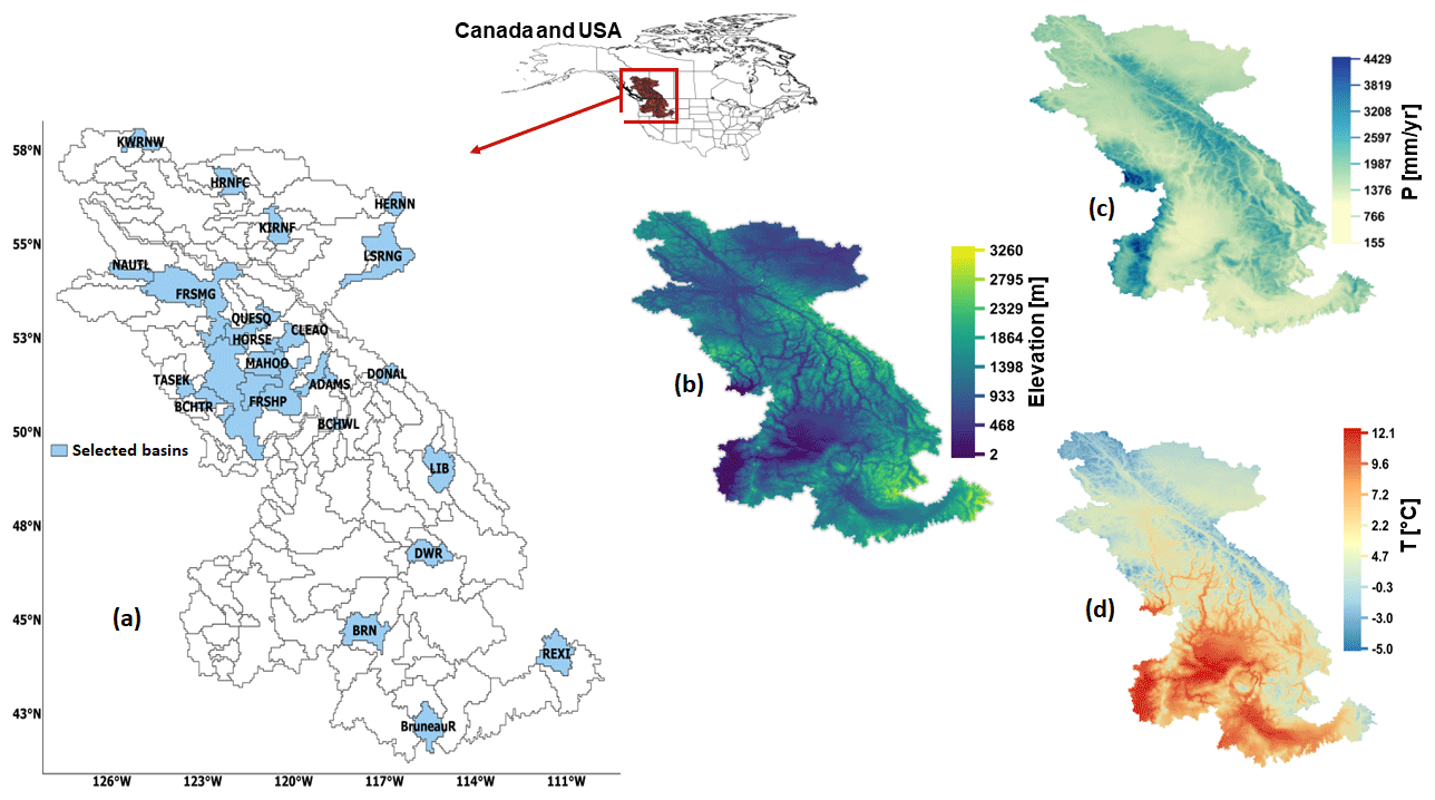
Figure 1 Modeled domain with the location of the 25 selected subbasins (a), the domain digital elevation map (b), mean annual precipitation (c) and mean annual temperature (d), which were calculated from the PNWNAmet dataset.

2.1 Study area and dataset

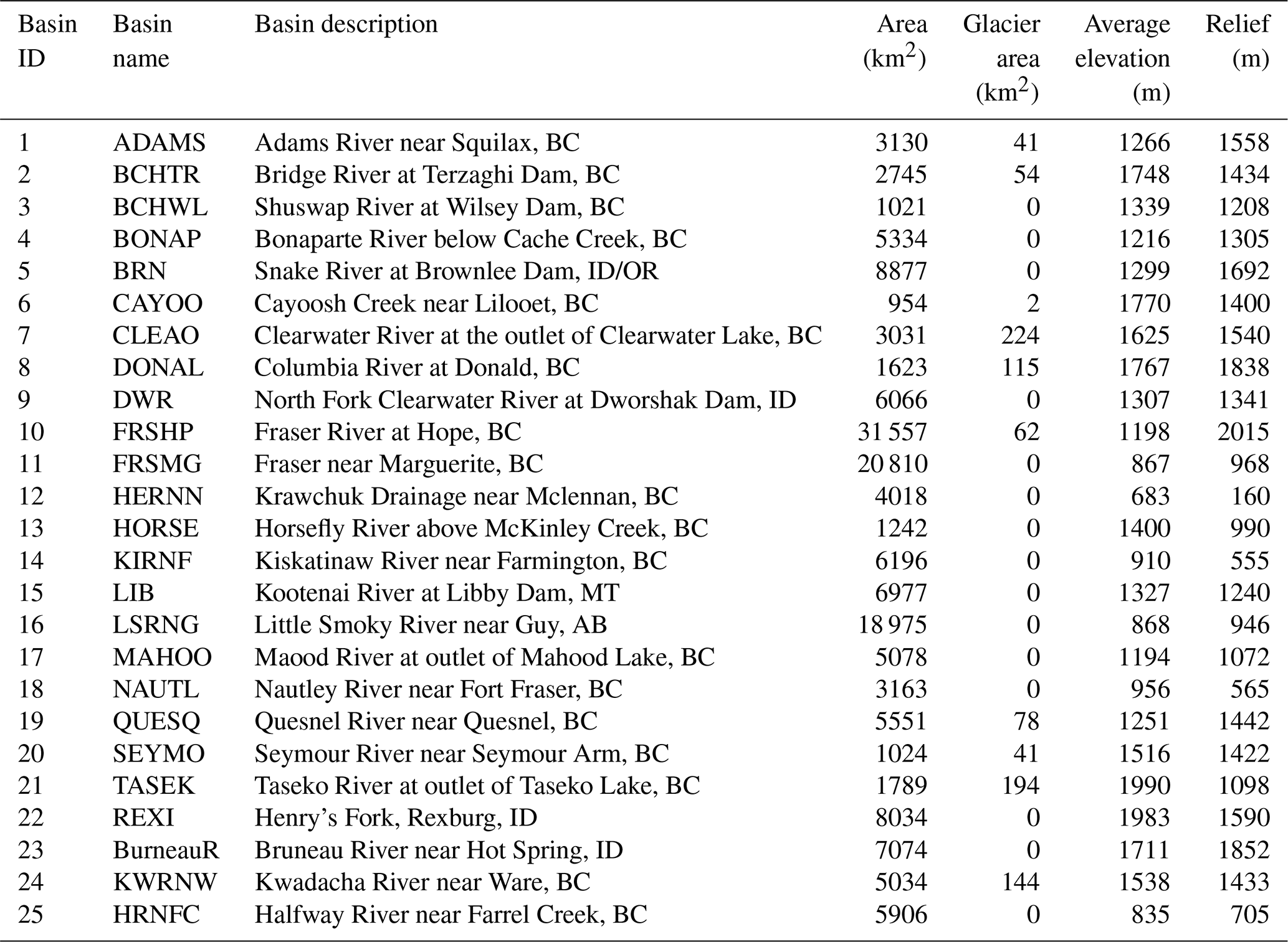
The study area extends over the Pacific Northwest region of North America from 40.75 to 57.6^∘ N and from 109.96 to 127.9^∘ W (see Fig. 1). It encompasses three large watersheds, the Peace, Fraser and Columbia rivers, with a combined area of 1 150 624 km². This region spans many physiographic and climatic zones, resulting in substantial hydroclimatic spatial variability. The domain was subdivided into several smaller basins (158 in total) according to the locations of hydrometric gauges. We selected 25 of these basins representing glacierized conditions in the Coast Mountains and the Rocky Mountains, semiarid conditions in the interior of both the Fraser and Columbia rivers and in the eastern Peace River, as well as arid conditions of the southern Columbia River. The locations of these basins are presented in Fig. 1, and their characteristics are summarized in Tables 1 and 2. The selected basins capture large spatial variability in precipitation, which is largely controlled by orography, such that average annual precipitation over the 25 basins ranges from 337 to 1666 mm yr⁻¹. The sampled basins also capture a strong latitudinal gradient of air temperature, with average annual temperature ranging from −0.37 to 7.43 ^∘C. The snow index, i.e., the fraction of annual precipitation that falls as snow when temperature is below 2 ^∘C (Woods, 2009; Sawicz et al., 2011), ranges from 0.38 to 0.70. The aridity index, i.e., the ratio of evapotranspiration to precipitation (ET$/P$), ranges from 0.28 to 1.66. Average catchment elevation ranges from 683 to 1990 m.

Table 1 Physiographic attributes of the 25 selected basins.

Table 2 Climatic attributes of the 25 selected basins.

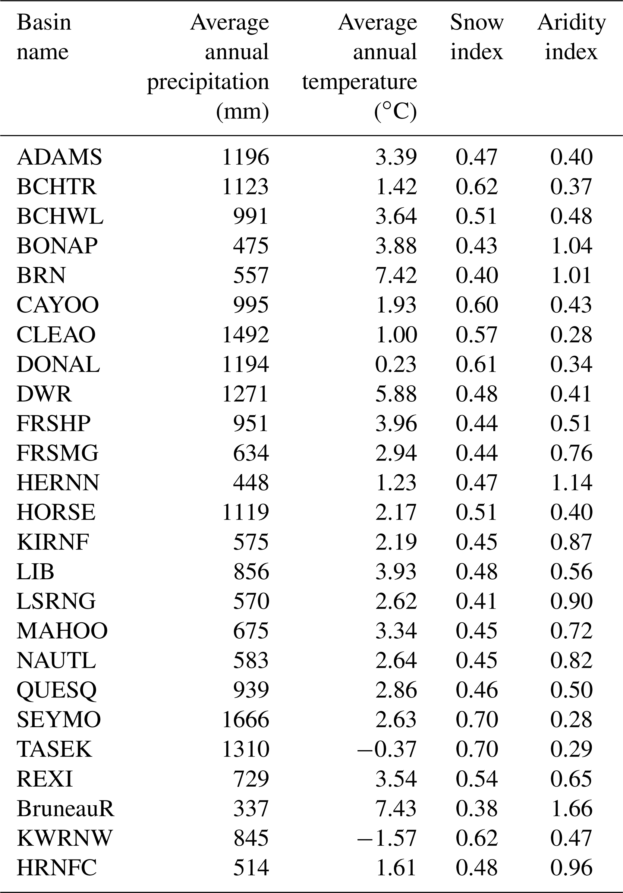
The climatic attributes presented in Table 2 are spatially averaged by subbasin from the gridded Pacific Climate Impacts Consortium's Northwest North America meteorology (PNWNAmet) dataset (Werner et al., 2019), which is used to drive the VIC model. This dataset provides gridded observations of daily precipitation (mm) and minimum and maximum temperature (^∘C) for northwestern North America. The dataset is available at a daily time step and a spatial resolution of $\mathrm{1}/\mathrm{16}$^∘ for the period 1945 to 2012. Wind speed (m s⁻¹) from the Twentieth Century Reanalysis (20CR) (Compo et al., 2011) that has been spatially interpolated to $\mathrm{1}/\mathrm{16}$^∘ is also provided with the PNWNAmet dataset at a daily timescale. For further details, see Werner et al. (2019).

2.2 VIC-GL model

VIC is a physically based macroscale model that simulates both water and energy balances by grid cells (Liang et al., 1994, 1996; Cherkauer and Lettenmaier, 1999). The VIC model has been widely applied to analyze the impact of climate change on the hydrology and water resources of the study region (e.g., Hamlet and Lettenmaier, 1999; Payne et al., 2004; Shrestha et al., 2012; Schnorbus et al., 2014; Islam et al., 2017) and to study the effect of land cover change on streamflow (e.g., Matheussen et al., 2000). VIC-GL, an upgraded version developed at the Pacific Climate Impacts Consortium (PCIC) that is used here, includes additional functionality to simulate glacier mass balance (Schnorbus, 2018). VIC-GL was branched from VIC version 4.2, and although the model physics are similar in many ways, it uses a different model abstraction from its predecessor. Although the computational domain of VIC-GL is still described using a two-dimensional grid (using a spatial resolution of $\mathrm{1}/\mathrm{16}$^∘ in the current application), subgrid variability in land cover and topography uses hydrologic response units (HRUs) as opposed to the original vegetation tiles. Specifically, an HRU is assigned for each land cover class within an elevation band, with the elevation of each HRU being the median of the associated elevation band. In this manner, the type and extent of the land cover are allowed to vary with elevation within grid boxes. The vertical water and energy balance is solved separately in each HRU and then averaged to the grid-cell scale. The current application of VIC-GL uses fixed 200 m elevation bands and three soil layers. The baseline model processes are described in detail by Liang et al. (1994, 1996), Cherkauer et al. (2003) and Bohn and Vivoni (2016).

Updates to address glacier mass balance modeling are described in detail by Schnorbus (2018), but pertinent VIC-GL parameter changes are summarized here. Glacier surface mass and energy balance modeling introduces three additional parameters: GLAC_ALB, GLAC_ROUGH and GLAC_REDF. GLAC_ALB specifies the albedo of glacier ice, which controls the amount of incoming solar radiation absorbed by the ice surface. The value of GLAC_ALB, once set, is constant in time. The parameter GLAC_ROUGH specifies the roughness length of the glacier surface, which affects the wind speed profile and the transfer of energy to the glacier surface due to the turbulent fluxes. The scaling factor for snow redistribution (GLAC_REDF) controls the redistribution of precipitation between non-glacier HRUs and acts as a proxy for mechanical snow redistribution that typically occurs via wind and gravity in mountainous alpine environments (e.g., Kuhn, 2003). VIC-GL also uses the rain–snow partitioning algorithm of Kienzle (2008) rather than the original algorithm in the VIC model distribution. This is a curvilinear model that uses two parameters, the threshold mean daily temperature (TEMP_TH_1, where 50 % of precipitation falls as snow) and the temperature range centered on TEMP_TH_1 within which both solid and liquid precipitation occurs (TEMP_TH_2). VIC-GL has also been updated to make certain parameters more accessible for model calibration and to allow for a more spatially explicit description of some hydroclimatic processes. These parameters include five that determine soil albedo decay according to the US Army Corps of Engineers (USACE) algorithm (USACE, 1956) and the climatic parameters T_LAPSE and PGRAD. The latter specify vertical temperature and the precipitation gradients that are used to adjust temperature and precipitation, respectively, for each HRU within a grid cell.

2.3 Model parameterization and sampling

We consider 44 VIC-GL parameters (Table 3) composed of 5 baseflow parameters, 1 runoff parameter, 9 drainage parameters, 4 climate parameters, 6 snow-related parameters, 3 glacier parameters and 17 vegetation-related parameters. The set of analyzed parameters includes the commonly calibrated parameters, parameters that have been addressed in previous studies (e.g., Demaria et al., 2007; Houle et al., 2017; Bennett et al., 2018) and some parameters that are typically set to fixed values (Gao et al., 2009, unpublished).

Table 3 The 44 VIC-GL parameters selected for the sensitivity analysis.

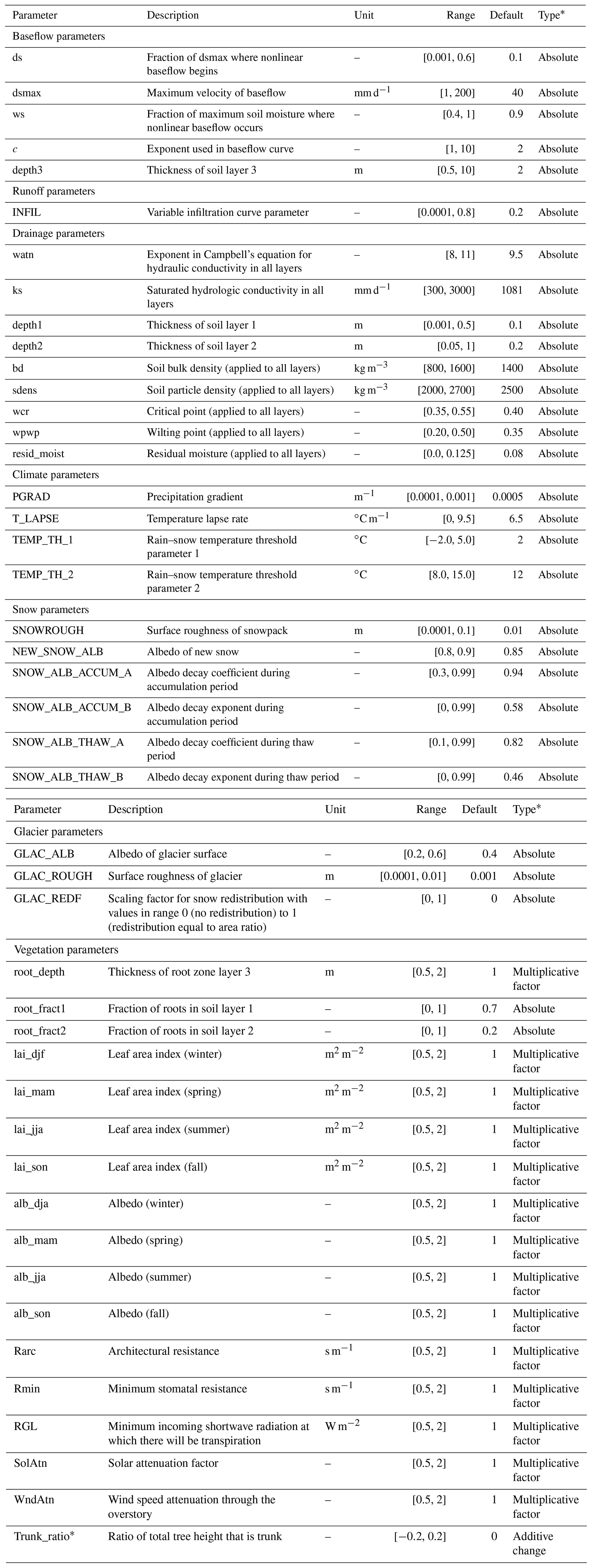
^* “Type” is the parameter sampling strategy, which is to either replace the parameter default value (i.e., “Absolute”), apply a multiplicative factor or apply an additive change to the baseline values. The additive change is applied so that the trunk ratio remains between 0.1 and 0.8.

The commonly calibrated parameters are limited to four baseflow parameters, the runoff parameter and five drainage parameters. The common baseflow parameters are the maximum velocity of baseflow (dsmax), the fraction of dsmax where nonlinear baseflow begins (ds), the fraction of maximum soil moisture where nonlinear baseflow occurs (ws) and the thickness of the deepest soil layer (depth3). These parameters describe the nonlinear relationship between baseflow rate and soil moisture in the deepest soil layer (with thickness described by depth3). The runoff parameter, or the variable infiltration curve parameter (INFIL), describes the extent of soil saturation within a grid cell (i.e., the amount of direct runoff) as a function of soil moisture in the surface soil layers (i.e., the variable infiltration curve: Liang et al., 1994), which have thicknesses given by depth1 and depth2. The common drainage parameters are the two parameters controlling soil storage capacity (depth1 and depth2), the exponent in Campbell's equation for hydraulic conductivity (watn) and the saturated hydrologic conductivity (ks).

The additional drainage parameters considered are the soil bulk density (bd), soil particle density (sdens), fractional soil moisture content at the critical point (wcr), fractional soil moisture content at the wilting point (wpwp) and the residual moisture (resid_moist). The wpwp parameter dictates baseflow estimation with the ARNO model formulation (Francini and Pacciani, 1991) used in VIC (Gao et al., 2009, unpublished). We also consider the four climate parameters, which are temperature lapse rate (T_LAPSE), precipitation gradient and the rain–snow temperature threshold parameters 1 and 2 (TEMP_TH_1, TEMP_TH_2). The examined parameters also include the three glacier mass balance parameters (GLAC_ALB, GLAC_ROUGH, GLAC_REDF). The snow-related parameters examined are surface roughness (SNOWROUGH), albedo of new snow (NEW_SNOW_ALB) and albedo decay parameters during the accumulation period (SNOW_ALB_ACCUM_A, SNOW_ALB_ACCUM_B) and during the thaw period (SNOW_ALB_THAW_A, SNOW_ALB_THAW_B).

The parameters describing snow and glacier properties along with soil and climate parameters are assigned by grid cell. These parameters were initialized with default values and then sampled within prescribed ranges (see Table 3). The same value is assigned to all grid cells within a catchment. The sampling of the soil parameters critical point (wcr), wilting point (wpwp) and residual moisture (resid_moist) is constrained so that conditions required by VIC (Gao et al., 2009, unpublished) are not violated. Thus, sampling is performed so that wcr ≤ (1 − bd$/$sdens), wpwp ≤ wcr and resid_moist ≤ wpwp × (1 − bd$/$sdens).

The vegetation parameters consist of the thickness of the root zone of the third soil layer (root_depth) and the root fractions in all three soil layers. We only sample root fractions in soil layers 1 and 2 (root_fract1, root_fract2) such that the total root fraction in the three soil layers adds up to 1. That is, the root fraction in soil layer 3 is updated as 1 − (root_fract1 + root_fract2). The vegetation parameters that are considered also include the seasonal leaf area index (lai), the seasonal albedo (albedo), the architectural resistance (Rarc), the minimum stomatal resistance (Rmin), the minimum incoming shortwave radiation at which there will be transpiration (RGL), the solar attenuation factor (SolAtn), wind speed attenuation through the overstory (WndAtn) and the fraction of the total tree height that is occupied by tree trunks (Trunk_ratio). The lai parameter governs the amount of water intercepted by the canopy, which controls canopy evaporation. Leaf area index, along with Rmin, also influences the estimation of vegetation transpiration, and the root fraction dictates the amount of transpiration from each soil layer (Gao et al., 2009, unpublished). The parameter Rarc affects the vertical wind profile.

The vegetation parameters are assigned by land cover class. Sampling of these parameters is conducted by adjusting baseline values obtained for each land cover class. The land cover classes were based on the North America Land Cover dataset, edition 2 (Natural Resources Canada/Canadian Centre for Remote Sensing (NRCan/CCRS) et al., 2013) produced as part of the North America Land Change Monitoring System (NALCMS). In total, 22 land cover classes were identified. For most of these parameters, sampling is conducted by applying a multiplication factor, sampled in the range 0.5 to 2.0, to the baseline values. The same sampled parameter is applied to all vegetation classes. To reduce the number of vegetation parameters, a multiplier factor is applied on a seasonal basis for the monthly parameters LAI and albedo, following a similar approach of Bennett et al. (2018). For example, lai_djf is the multiplier factor applied to leaf area index values during winter months (i.e., December, January and February). The trunk ratio is sampled around the defined value by applying an additive change in the range −0.2 to 0.2 so that trunk ratio values remain between 0.1 and 0.8. The monthly roughness and displacement height parameters were not sampled. They are specified as a function of vegetation height (which is constant within classes but variable between classes) and leaf area index as described by Choudhury and Monteith (1988).

2.4 Sensitivity analysis

We applied the EEE screening method introduced by Cuntz et al. (2015) as a frugal implementation of the Morris method (Morris, 1991). It was developed to identify the model parameters that are most informative regarding a certain model output. The strength of the method lies in it requiring only a small set of model evaluations to separate informative vs. noninformative parameters. On average, EEE requires 10N model runs, with N being the number of model parameters. EEE does not require algorithmic tuning and converges by itself. The method was tested for a large range of sensitivity benchmarking functions and a hydrologic model at several locations by Cuntz et al. (2015). The method was further applied to obtain the informative parameters in complex hydrologic (Cuntz et al., 2016) and land surface models (Demirel et al., 2018).

The EEE approach samples model parameters in trajectories as initially described by Morris (1991) and improved by Campolongo et al. (2007). A “trajectory” is defined as a sequence of (N+1) parameter sets where the first parameter set is sampled randomly, while all subsequent sets i (i>1) differ from the prior set (i−1) in exactly one parameter value. Such trajectories allow an efficient sampling of the whole parameter space while considering parameter interactions to a certain extent. In the approach of Cuntz et al. (2015), only a small number of such trajectories (M₁; here M₁=5) are sampled in a first EEE iteration to lower the computational burden. The resulting ($M_{\mathrm{1}}\times (N+\mathrm{1})$) model outputs are derived, and the elementary effects (EEs) are computed for each parameter following Morris (1991). The EE quantifies the change in model output f(p) when a parameter p_i is changed by a fraction of this parameter range Δ. The elementary effect of parameter p_i is calculated as follows:

$$\begin{array}{}\text{(1)}& {\mathrm{EE}}_i={\displaystyle \frac{f\left(p_i+\mathrm{\Delta }\right)-f\left(p_i\right)}{\mathrm{\Delta }}}.\end{array}$$

The EEs are used to identify the most informative parameters by deriving a threshold that splits the parameters into a set of N_ninf noninformative parameters and a set of $N_{\inf }=N-N_{\mathrm{ninif}}$ informative parameters. The threshold T is derived automatically within the EEE method and is based on the EEs of the model outputs provided in the first iteration. The threshold is derived based on fitting a logistic function to the sorted EEs derived and defining the threshold as the point of largest curvature of the fitted logistic function. Defining the threshold that is used to separate informative and noninformative parameters in this approach has been demonstrated using a wide range of test functions and real-world examples, and the reader is referred to Cuntz et al. (2015) for further details. In the next EEE iteration, a new N-dimensional parameter set is randomly sampled, but this time only the N_ninf noninformative parameters are perturbed, while the N_inf informative parameters are kept at their initially sampled values. Hence, this trajectory contains only N_ninf+1 parameter sets. M₂ parameter sets of such trajectories are sampled in this step (here M₂=1). The derivation of model outputs and the calculation of EEs are repeated. If the EE of any noninformative parameter exceeds the previously derived threshold T, the previously noninformative parameter will be added to the set of informative parameters. This EEE iteration (sampling a new trajectory and then adding parameters with an EE above T to the set of informative parameters) is repeated until no further parameter is reclassified as informative. The final EEE iteration is to sample M₃ trajectories (here M₃=5) to confirm that the set of N_ninf noninformative parameters is stable, and no further parameter is found to be informative. The EEE method's parameter values (M₁, M₂ and M₃) utilized here are the default settings tested and recommended by Cuntz et al. (2015). The implementation, documentation and examples for EEE are open source (Mai and Cuntz, 2020).

2.5 Transferability of parameter sensitivity

We applied the EEE method to each of the 25 basins and the three model outputs (streamflow, evaporation, snow water equivalent) independently, leading to 75 sets of noninformative and informative parameters. The initial set of N randomly sampled model parameter values was the same for all 75 experiments. An average of 430 model runs were required for all 75 EEE experiments to identify which of the 44 VIC-GL parameters analyzed in this study were informative.

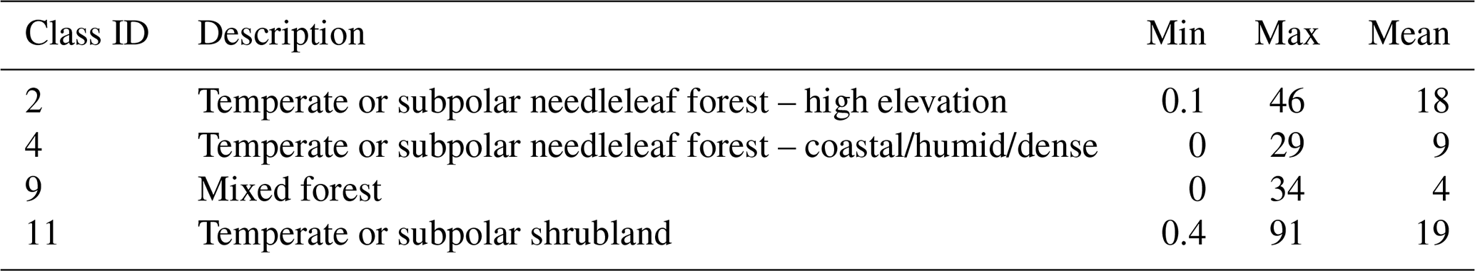
Table 4 Statistics of the percentage of VIC land cover classes (%) identified using NALCMS and considered in this study over the 25 selected basins.

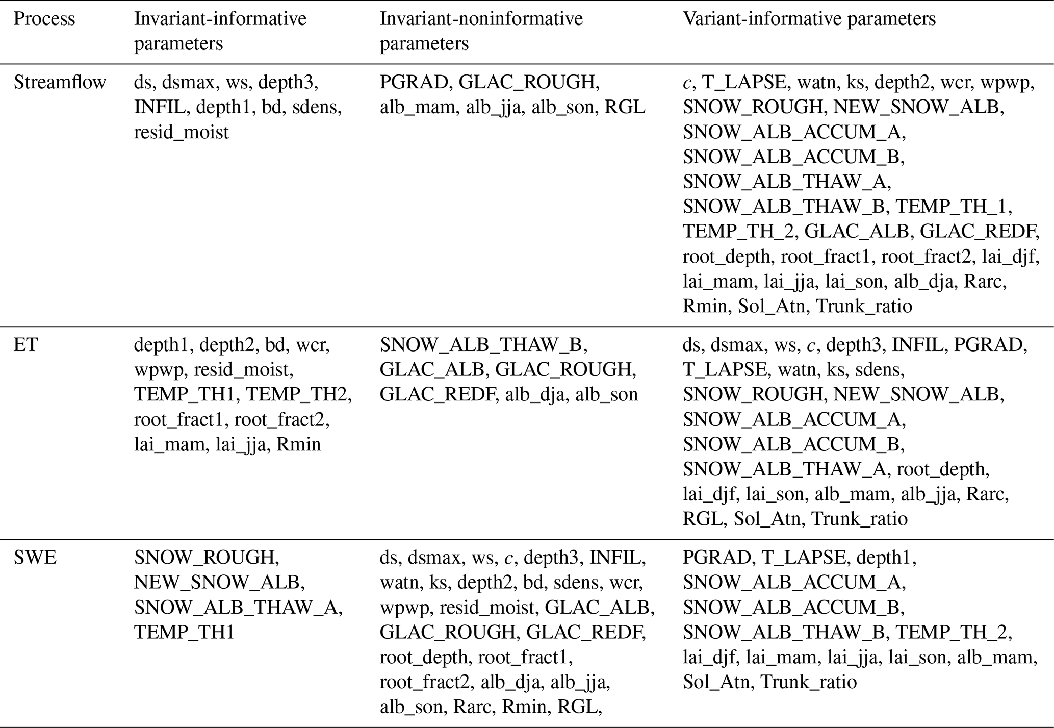
Informative and noninformative parameters were compared over the 25 basins to identify (1) parameters that are informative across all basins (termed invariant-informative parameters), (2) parameters that are noninformative across all basins (invariant-noninformative) and (3) parameters that are informative in some basins but not others (variant-informative).

We evaluated the potential of using watershed classification as a tool to transfer parameter SA information. Climatic conditions exert a major control on runoff generation (Yadav et al., 2007; Sawicz et al., 2011) and have been found to have a higher impact on parameter sensitivity than vegetation and soil conditions (Rosero et al., 2010). However, vegetation and soil conditions can affect other hydrologic quantities. For example, Bennett et al. (2018) found that canopy spacing plays an important role in snow water equivalent simulation by VIC. Here, we used aridity index, snow index and the percentage of glacier area as well as the percentage of area covered by each of several vegetation classes to classify the 25 basins. Although 22 vegetation classes are defined for VIC-GL, we only considered the 4 vegetation classes listed in Table 4 that are dominant in the study area. To evaluate the impact of vegetation on informative parameter identification, watershed classification was first performed by using the climatic attributes only and then by combining climatic and vegetation class cover attributes.

To classify the 25 basins into homogenous groups, the agglomerative hierarchical algorithm was used with the Euclidean distance and Ward's criterion (Roux, 2018). Agglomerative hierarchical clustering consists of a series of successive fusions of watersheds into groups according to their similarity. It starts by considering each element x (i.e., watershed) as a cluster {x} and then continues by creating a new cluster by merging the two closest clusters. The dendogram, a tree diagram, illustrates the merging process of the agglomerative hierarchical clustering. The Ward method used here aggregates clusters so that within-group inertia (i.e., multi-dimensional variance) is minimal.

To test our hypothesis that parameter sensitivity can be generalized using watershed classification, we conducted the following evaluation. Each subbasin was set as the target basin. For each target basin, informative parameters are transferred using a number of donor basins of the same cluster. Using multiple donor basins has been shown to provide better results than a single donor basin (e.g., Oudin et al., 2008; Bao et al., 2012). Let A be a target basin of cluster C_i. We assume that informative parameters of basin A are the intersection of informative parameters of x donor basins from cluster C_i. For each target basin A, informative parameters are transferred using all possible combinations of x donor basins of cluster C_i not including A. This test aims at evaluating whether x donor basins could be used to generalize informative parameters for each cluster.

The performance of watershed classification in identifying informative and noninformative parameters in a basin is evaluated using the F1 score. This score is often used to measure the performance of a binary classification (Chicco and Jurman, 2020). The F1 score is a weighted average of precision and recall. Assuming two classes, positive (informative) and negative (noninformative), the F1 score measures the ability to correctly and incorrectly predict the two classes. Considering counts of TP (true positive, i.e., informative predicted as informative), FP (false positive, i.e., informative predicted as noninformative) and FN (false negative, i.e., noninformative predicted as informative), we can obtain measures of precision, recall and the F1 score as follows:

$$\begin{array}{}\text{(2)}& {\displaystyle }& {\displaystyle }\mathrm{Precision}={\displaystyle \frac{\mathrm{TP}}{\mathrm{TP}+\mathrm{FP}}},\text{(3)}& {\displaystyle }& {\displaystyle }\mathrm{Recall}={\displaystyle \frac{\mathrm{TP}}{\mathrm{TP}+\mathrm{FN}}},\text{(4)}& {\displaystyle }& {\displaystyle }\mathrm{F}\mathrm{1}\mathrm{score}=\mathrm{2}\cdot {\displaystyle \frac{\mathrm{precision}\times \mathrm{recall}}{\mathrm{precision}+\mathrm{recall}}}.\end{array}$$

The F1 score takes values between 0 and 1, where 0 means that all positive (here informative parameters) are predicted as negative (i.e., as noninformative) and 1 means perfect classification with FN = FP = 0.

For a given number of donor basins x, the F1 score is reported for each target basin A as the average F1 score calculated between sensitive parameters of A and identified sensitive parameters from all possible combinations of the x donor basins. This is done for each classification method as well as climate-based and climate–land-cover-based clustering to evaluate performance in identifying sensitive parameters by watershed groupings provided by each clustering analysis. Then, we use the Wilcoxon signed rank test to compare the F1 scores for the 25 basins obtained using the two clustering methods so that we can determine whether incorporating land cover into watershed classification improves the ability to predict informative parameters. The Wilcoxon signed rank test tests the null hypothesis that the F1 scores resulting from both clustering analyses are from the same distribution, i.e., that they have similar abilities to identify informative parameters.

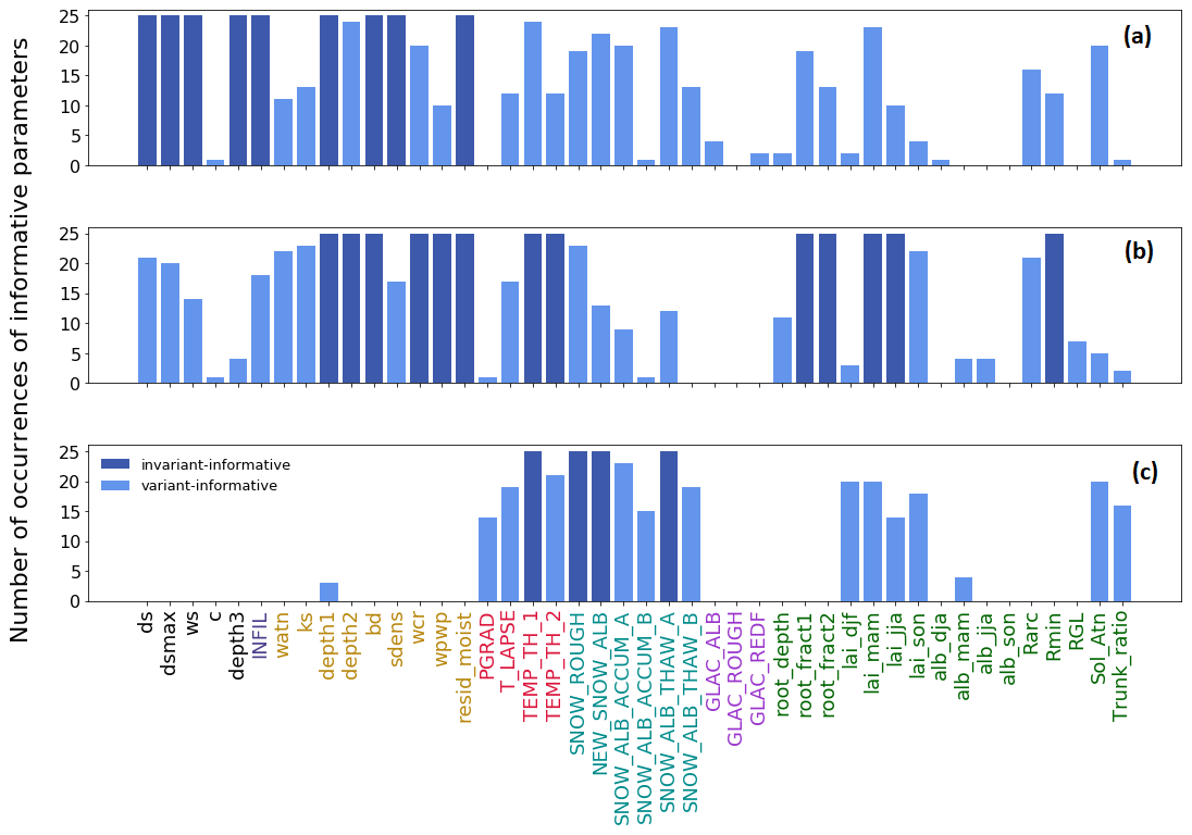
Figure 2 Number of occurrences of informative parameters for streamflow (a), evapotranspiration (b) and snow water equivalent (c) over the 25 studied subbasins. Parameters are considered invariant-informative if the count of basins in which they are informative equals 25, invariant-noninformative if that count is 0, and variant-informative if the count is between 1 and 24.

3 Results

The sensitivity analysis using the EEE method was performed independently with respect to three model outputs: streamflow, evapotranspiration and snow water equivalent. Figure 2 presents the number of occurrences of informative parameters over the 25 selected subbasins for the three outputs. From this figure, we can identify the three parameter categories invariant-informative, invariant-noninformative and variant-informative for each hydrologic process. Table 5 summarizes the three parameter categories per model output. Amongst the 44 VIC-GL parameters, only 9 parameters are invariant-informative for streamflow, 13 are invariant-informative for evapotranspiration and 4 are invariant-informative for snow water equivalent. A large percentage of parameters are variant-informative for these fluxes, with 29 parameters for streamflow, 25 parameters for evapotranspiration and 14 parameters for snow water equivalent. We first examine the sensitive parameters and their spatial variability per model output in Sect. 3.1 to 3.3. We further analyze the performance of the physical similarity approach for transferring sensitivity analysis information and the attributes that are informative for each model output (Sect. 3.5).

Table 5 VIC-GL parameter importance regarding streamflow, evapotranspiration (ET) and snow water equivalent (SWE).

3.1 Informative parameters for streamflow

The soil parameters ds, dsmax, ws, depth3 and depth1 are consistently identified as sensitive to streamflow (e.g., Demaria et al., 2007; Bennett et al., 2018; Gou et al., 2020), and this reflects the empirical nature of the runoff and baseflow processes that are fundamental in the VIC family of models. In addition to these parameters, the soil parameters soil bulk density (bd), soil particle density (sdens) and residual moisture (resid_moist) are also identified as invariant-informative on streamflow in the study area.

Figure 3 presents the sensitivity of the 29 variant-sensitive parameters with respect to streamflow (Table 5). These parameters include the remaining soil parameters, climate, snow and most of the vegetation parameters. The climate parameters TEMP_TH_1 and TEMP_TH_2 (i.e., the rain–snow temperature threshold parameters 1 and 2) have different sensitivity patterns. The parameter TEMP_TH_1 is found to be informative across all the basins except in the arid basin BruneauR, which has the lowest snow index (0.38). The parameter TEMP_TH_2 is informative only in subbasins located in the interiors of the Fraser and Peace basins. T_LAPSE is informative in the snow-dominated basins of the Fraser and Columbia rivers. The snow-related parameters show different spatial sensitivities. For instance, SNOW_ROUGH is sensitive over all the basins except for some snow-dominated basins of the Fraser and Columbia rivers. NEW_SNOW_ALB and SNOW_ALB_THAW_A, which control snowmelt, are sensitive across all the basins except the semiarid basins of the Peace River (northeast of the study region). Snowmelt in the study area contributes significantly to runoff, which explains the sensitivity of these parameters for streamflow. These results are consistent with the results found by Houle et al. (2017), who evaluated the sensitivity of these parameters to snow water equivalent using the Sobol' method (Sobol', 1990).

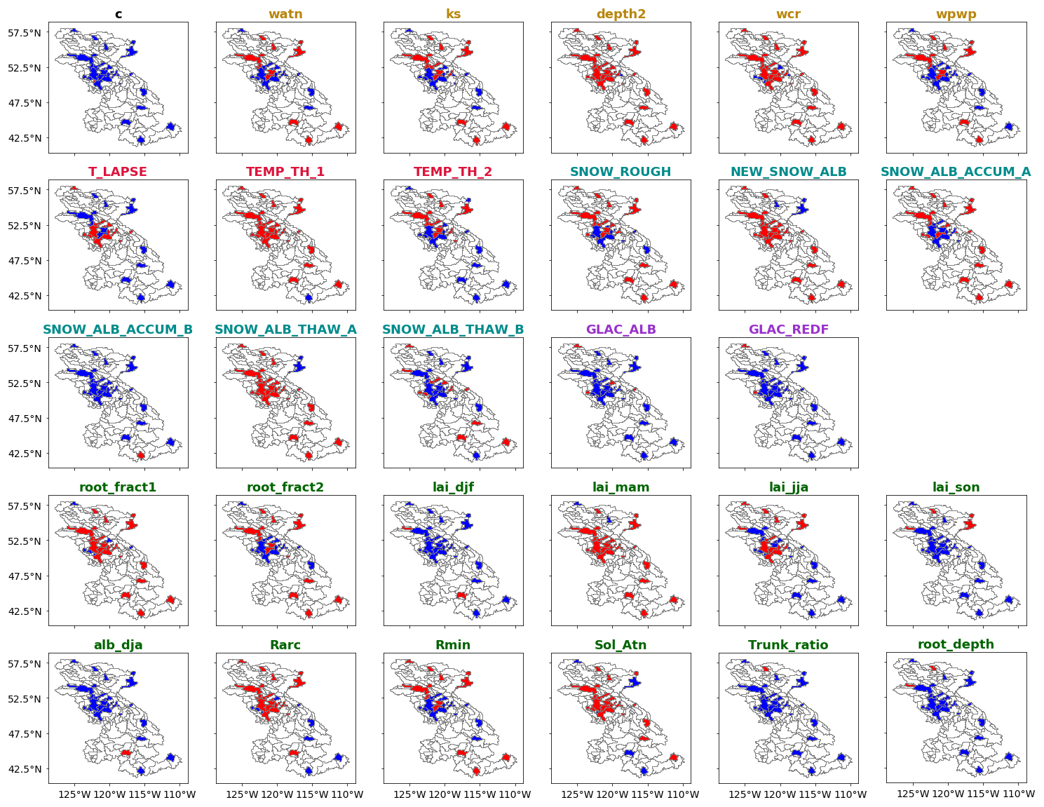
Figure 3 The spatial sensitivity of the 29 streamflow variant-informative parameters, with red being informative and blue noninformative over the 25 selected basins. The nine invariant-informative and six invariant-noninformative parameters are not included.

In the semiarid and arid basins, the exponent in Campbell's equation for hydraulic conductivity (watn), the saturated hydrologic conductivity (ks) and the fractional soil moisture content at the wilting point (wpwp) are informative for streamflow. The wpwp parameter dictates baseflow estimation with the ARNO model formulation (Francini and Pacciani, 1991) used in VIC (Gao et al., 2009, unpublished). Given the limited precipitation in these basins, baseflow may be a significant streamflow source that explains the importance of this parameter in these basins. The root depth of the third layer (root_depth) is sensitive in the northern semiarid basins (NAUTL, HRNFC). The root fraction of the first layer (root_fract1) is sensitive in the Columbia basins and the non-glacierized basins of the Fraser and Peace rivers. The root fraction in the second layer (root_fract2) is sensitive only in the semiarid and arid basins. The sensitivity of the LAI parameters is seasonal, with springtime LAI being sensitive in almost all the basins.

For the glacierized headwater catchments, the albedo of the glacier surface (GLAC_ALB) is informative for streamflow. The importance of this parameter increases with the basin glacier area, and this parameter is influential in the four basins CLEAO, KWRNW, DONAL and TASEK with the largest glacier area (between 115 and 194 km², i.e., between 7 % and 11 % of the watershed area). The remaining glacierized basins have much smaller glacier areas (less than 1.5 % of the watershed area). The GLAC_REDF parameter is also informative for streamflow in the western-glaciated basins TASEK and KWRNW, where the average annual temperature is negative. Glaciers behave as natural water reservoirs that provide streamflow through ice melt and temporary meltwater storage within the glacier during late summer (Marshall et al., 2011). For instance, in the upper Columbia River, glaciers contribute up to 25 % and 35 % of streamflow in August and September, respectively, and up to 6 % to the annual streamflow (Jost et al., 2012; Jiskoot and Mueller, 2012).

3.2 Informative parameters for evapotranspiration

There are 13 invariant-informative parameters that affect evapotranspiration in the study region (see Fig. 2 and Table 5). These include parameters that control soil drainage (wcr, wpwp and resid_moist) and soil storage capacity (bd, depth1 and depth2). The invariant-informative parameters also include the climate parameters (TEMP_TH_1, EMP_TH_2), vegetation parameters seasonal leaf area indices (lai_mam, lai_jja), minimum stomatal resistance (Rmin) and root fractions (root_fract1, root_fract2). The VIC-GL model computes evapotranspiration as the sum of four types of evaporation: evaporation from the canopy layer, transpiration from all three soil layers, soil evaporation from the top soil layer and evaporation or sublimation from the snow or glacier surface (Liang et al., 1994). The soil parameters affect the bare soil evaporation that occurs in the top thin layer. The leaf area index parameters govern the amount of water intercepted by the canopy, which controls canopy evaporation. Leaf area index and Rmin influence the estimation of vegetation transpiration, and the root fraction dictates the amount of transpiration from each soil layer (Gao et al., 2009, unpublished). These parameters are defined for each land cover type in the vegetation library. They are typically fixed based on observed values, which ignores the large estimation and scaling uncertainties around their values (Mendoza et al., 2015). In this paper, the sampling of LAI and Rmin values is based on a perturbation of observed values (see Table 3; type “Multiplicative factor”). The sensitivity of evapotranspiration to this perturbation illustrates the need to obtain accurate values for these parameters or to consider their uncertainty in the model calibration process. The rain–snow temperature thresholds (TEMP_TH_1, TEMP_TH_2) are likely to impact the throughfall (water that penetrates a plant canopy) and rainfall–snow interception (rain captured, stored and evaporated from the vegetation surface) (Levia et al., 2019).

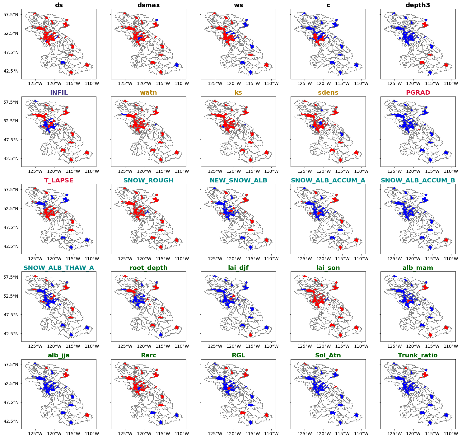
Figure 4 The spatial sensitivity of the 25 evapotranspiration variant-informative parameters, with red being informative and blue noninformative over the 25 selected basins. The 13 invariant informative and 6 invariant-noninformative parameters are not included. For the number of occurrences of informative parameters, see Fig. 2.

Table 5 lists the six invariant-noninformative parameters for evapotranspiration, which are the glacier parameters, fall and winter vegetation albedo as well as the albedo decay exponent during the thaw period SNOW_ALB_THAW_B. Figure 4 presents the spatial sensitivity of the 25 variant-informative parameters with respect to evapotranspiration. Some parameters show a clear spatial pattern of sensitivity that is related to basin physical characteristics. For instance, T_LAPSE is sensitive in snow-dominated basins, whereas INFIL and sdens are sensitive in semiarid and arid basins. The baseflow parameters (ds, dsmax) are informative in most basins, while the parameter ws is only informative in humid subbasins. The surface roughness of the snowpack (SNOW_ROUGH), the architectural resistance of vegetation (Rarc, which affects the vertical wind profile) and the fall leaf area index (lai_son) are also influential in evapotranspiration in most basins.

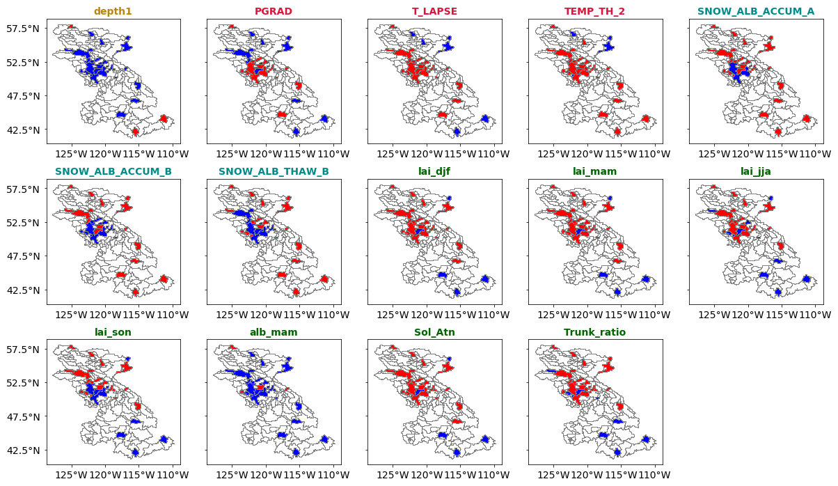
Figure 5 The spatial sensitivity of the 14 snow water equivalent variant-informative parameters, with red being informative and blue noninformative over the 25 selected basins. The 4 invariant informative and 26 invariant-noninformative parameters are not included. For the number of occurrences of informative parameters, see Fig. 2.

3.3 Informative parameters for snow water equivalent

Amongst the six snow parameters, only three (SNOW_ROUGH, NEW_SNOW_ALB, SNOW_ALB_THAW_A) are invariant-informative for snow water equivalent. The climate parameter TEMP_TH_1 is also invariant-informative for snow water equivalent. The parameter TEMP_TH_2 is informative in the majority of the basins, except in the semiarid basins of the Peace River. The sensitivity of the remaining three snow parameters (SNOW_ALB_ACCUM_A, SNOW_ALB_ACCUM_B, SNOW_ALB_THAW_B) and the two climate parameters (PGRAD, T_LAPSE) varies within the study region. Figure 5 presents the sensitivity of the 14 variant-informative parameters for snow water equivalent. T_LAPSE and PGRAD are sensitive in the high-altitude basins. The parameter SNOW_ALB_ACCUM_B is informative in the basins of the Columbia and Peace rivers and in the semiarid basins of the Fraser River. The sensitivities of the seasonal leaf area index (lai_djf, lai_mam, lai_jja, lai_son), the ratio of total tree height that is trunk (Trunk_ratio) and the solar attenuation factor (Sol_Atn) show a clear spatial pattern. These parameters are informative in basins where forest is the dominant land cover (i.e., the Fraser and Peace rivers). The springtime vegetation albedo (alb_mam) is sensitive over the snow-dominated basins. The sensitivity of snow water equivalent for vegetation parameters can be explained by the impact of forest cover on snow accumulation and ablation processes, mainly by snowfall interception and modification of incoming radiation and wind speed below the forest canopy (Andreadis et al., 2009). These findings are consistent with those of Houle et al. (2017) and Bennett et al. (2018).

3.4 Watershed classification

Figure 6 presents the dendogram, a diagram tree of clusters resulting from the agglomerative hierarchical clustering using climate indices and the combination of climate indices and vegetation class cover. Clustering based on climate indices yields four clusters, whereas clustering based on climate indices and vegetation cover results in five clusters.

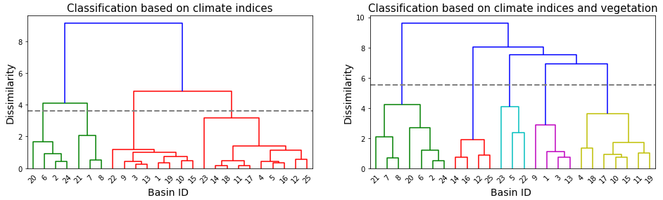
Figure 6 Watershed classification dendogram using climate indices and the combination of climate and vegetation indices. The height of each node represents the distance between its branches, and the dashed line represents the cutoff threshold to distinguish the four clusters in the case of climate-based classification and five clusters in the case of climate–land-cover-based classification. The threshold is chosen as a tradeoff between cluster dissimilarity and within-cluster variance.

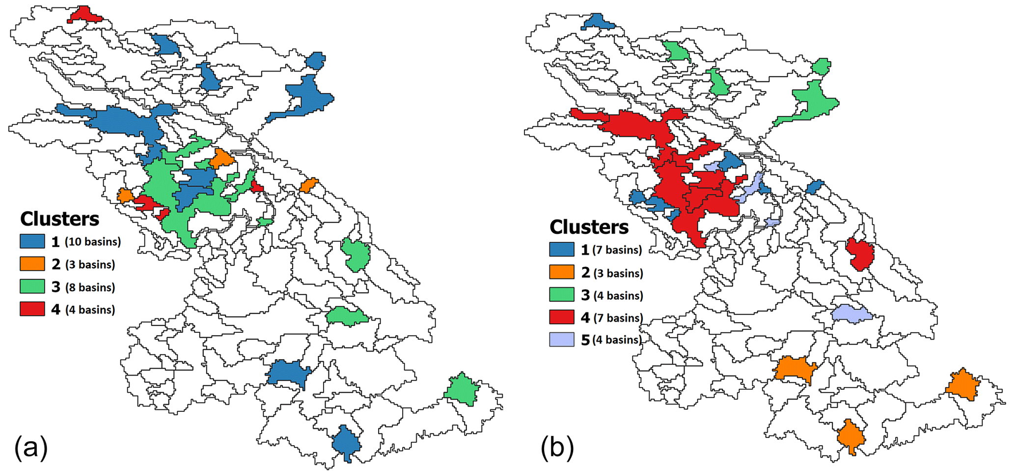
Figure 7 Map of clusters obtained using only climatic attributes (a) and using both vegetation and climatic attributes (b).

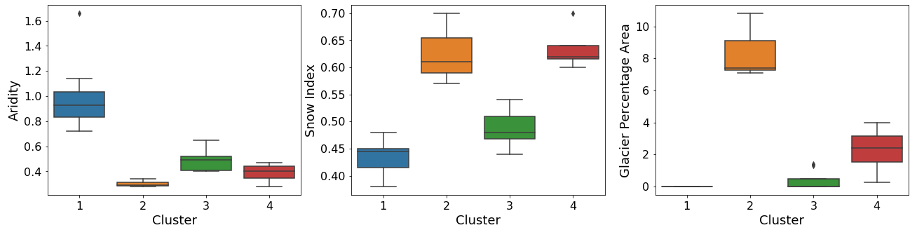
Figure 8 Boxplots of the climate attributes for each cluster produced by climate-based classification.

Figure 7 shows the results of the hierarchical clustering analyses, and Figs. 8 and 9 present the attribute statistics for each cluster. The clusters produced using climatic attributes can be described as follows. Cluster no. 1 consists of dry basins located in the southern Columbia, eastern Peace and central Fraser basins. Cluster no. 2 contains glacierized watersheds along the Coast Mountains and the Rocky Mountains. Cluster no. 3 contains semiarid basins in the interior Fraser and eastern Columbia basins, and Cluster no. 4 contains snow-dominated basins with a very low glacier area (less than 4 % of the watershed area) compared to Cluster no. 2. Clusters obtained using both climatic and vegetation attributes correspond to clusters based on climate that were merged or divided based on vegetation class cover dominance. Cluster no. 1 contains all glaciered watersheds and corresponds to Cluster nos. 2 and 4 obtained with climatic-based clustering. Cluster no. 2 consists of dry basins dominated by land cover 11 (temperate or subpolar shrubland) that are located in the southern Columbia basin. Cluster no. 3 consists of dry basins dominated by land cover 9 (i.e., mixed forest) located in the eastern Peace River basin. Cluster no. 4 represents arid basins in the interior Fraser and upper Columbia rivers dominated by land cover 2 (i.e., temperate or subpolar needleleaf forest – high elevation), and Cluster no. 5 consists of wet basins dominated by land cover 4 (i.e., temperate or subpolar needleleaf forest – coastal, humid or dense).

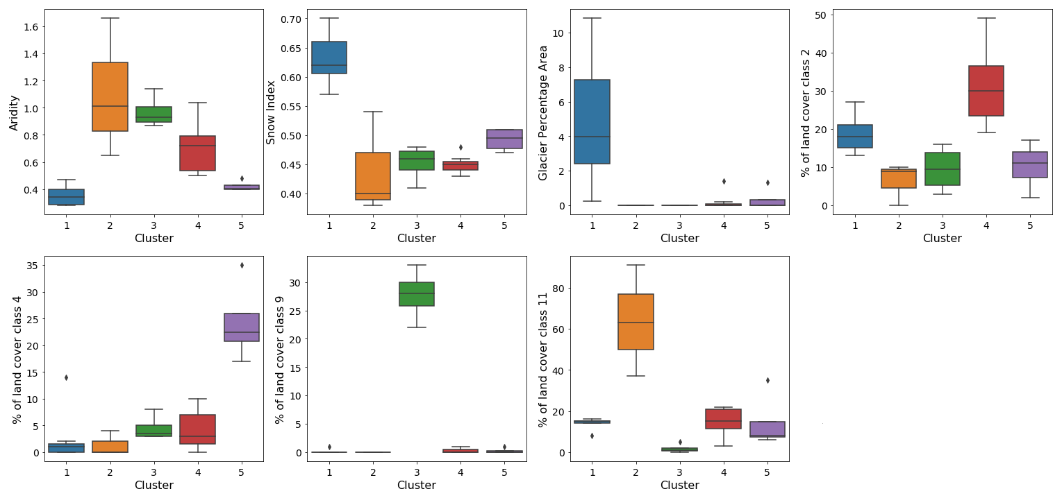
Figure 9 Boxplots of attributes of each cluster produced by climate- and vegetation-based classification.

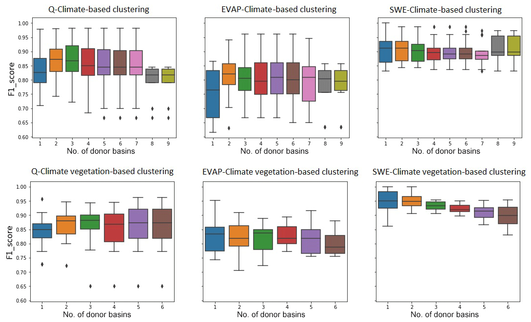
Figure 10 F1 score distribution obtained by transferring informative parameters over the 25 basins.

3.5 Watershed classification as a way to transfer parameter sensitivity

The distribution of F1 scores obtained by transferring informative parameters for streamflow, evaporation and snow water equivalent using both clustering analyses and a range of donor basins is presented in Fig. 10. The F1 scores calculated for transferring streamflow-informative parameters based on climatic attributes range between 0.66 (using nine donor basins) and 0.98 (using between three and seven donor basins), whereas this score ranges between 0.65 (using six donor basins) and 0.96 (using six donor basins) when using both climate and vegetation attributes. For evapotranspiration, the F1 scores are obtained by climatic-based clustering ranging between 0.63 (using six donor basins) and 0.96 (using three to six donor basins). The scores range between 0.7 (using two donor basins) and 0.95 (using a single donor basin) when using both climatic and land cover attributes for clustering analysis. The F1 scores for snow water equivalent range between 0.83 (using four to nine donor basins) and 1 (using one to two donor basins) when transferring informative parameters based on climatic attributes and the combination of climatic attributes and vegetation.

Transferring informative parameters based on more than a single donor basin improves the F1 score except when transferring evapotranspiration informative parameters using climatic and vegetation clustering analysis. Overall, the results show that two donor basins would be sufficient to generalize informative parameters to each cluster. Therefore, for each model output, we compare the F1 distributions using two donor basins based on both clustering analyses with the Wilcoxon test. The p value of the test applied to F1 score distributions obtained by transferring streamflow informative parameters is 0.49, and by transferring evapotranspiration informative parameters, it is 0.48. Hence, the F1 score distributions using climatic clustering analysis and climatic–land cover analysis are not significantly different. Therefore, using only climatic attributes would be sufficient to transfer informative parameters to streamflow and evapotranspiration. These findings are consistent with other VIC studies (Demaria et al., 2007) and other hydrologic models (e.g., Rosero et al., 2010) showing that parameter sensitivity for streamflow can be transferred based predominantly on climate similarity.

The Wilcoxon test statistic applied to the F1 distribution resulting from transferring snow water equivalent informative parameters is 31 with a p value of 0.0006. This suggests that there is a significant improvement when using both climatic and land cover attributes to transfer snow water equivalent parameter sensitivity. The importance of land cover and vegetation properties as a control on snow accumulation and ablation is consistent with previous studies (e.g., Bennett et al., 2018).

4 Discussion

In this work, we have examined the sensitivity of an extensive list of VIC parameters to streamflow, evapotranspiration and snow water equivalent over 25 basins spanning a range of hydroclimatic conditions. We found that informative parameters vary spatially with climate and land cover depending on the model output considered. The findings are in line with previous VIC sensitivity analysis studies (e.g., Demaria et al., 2007; Bennett et al., 2018; Gou et al., 2020; Sepúlveda, 2022). In addition, the two climate parameters temperature lapse rate (T_LAPSE) and precipitation gradient (PGRAD) omitted in previous studies have been found to be informative on headwater glacierized watersheds and snow-dominated non-glacierized watersheds. The T_LAPSE parameter is typically fixed when developing gridded meteorological data. For instance, Bohn and Vivoni (2016) used a gridded temperature corrected with a lapse rate of 6.5^∘ K km⁻¹ to force VIC over the southwestern US and northwestern Mexico. However, several studies have indicated that the often-used constant lapse rates 6–6.5 ^∘C km⁻¹ are not representative of the surface conditions over different mountainous regions and may differ for each slope within the same mountain (Blandford et al., 2008; Minder et al., 2010, Córdova et al., 2016).

In this study, we showed that watershed classification helps identify spatial patterns of informative parameters at a reduced cost. Hence, it reduces the cost of performing sensitivity analysis at the same scale of large-scale land surface models. In our case, watershed classification based on climatic attributes (snow index and aridity index) and percentage of glacier area was sufficient to transfer parameter sensitivity between basins of similar attributes. However, incorporating vegetation class cover significantly improved the identification of sensitive parameters for snow water equivalent. The results show that two donor basins per cluster are sufficient to identify sensitive parameters. These results imply that the cost of running a sensitivity analysis over a large domain encompassing N clusters of basins would be reduced to the cost of running 2N sensitivity analyses. The information gained can then be extrapolated to a large domain based on subwatershed membership to the N clusters. Thus, candidate parameters for model calibration can be identified at a substantially reduced computational cost as compared to running a large-domain sensitivity analysis. For example, climatic-based classification of the 158 basins that covers the entire domain results in four watershed clusters (see Fig. 11) as follows. Cluster no. 1 consists of glaciered basins along the Coast Mountains and the Rocky Mountains. Cluster no. 2 groups dry basins located in the interior and southern Columbia, eastern Peace and upper Fraser basins. Cluster no. 3 contains snow-dominated basins in the northern Peace River basin and the eastern Columbia River basin, whereas Cluster no. 4 contains rainfall-dominated basins in the western Columbia River basin. These clusters are consistent with the clusters obtained by classifying the 25 basins (except for Cluster no. 4) because the sample of the studied basins does not include any rainfall-dominated basins. Hence, the cost of performing a sensitivity analysis across the 158 basins is reduced to the cost of evaluating parameter sensitivity over eight basins (i.e., two basins for each basin cluster).

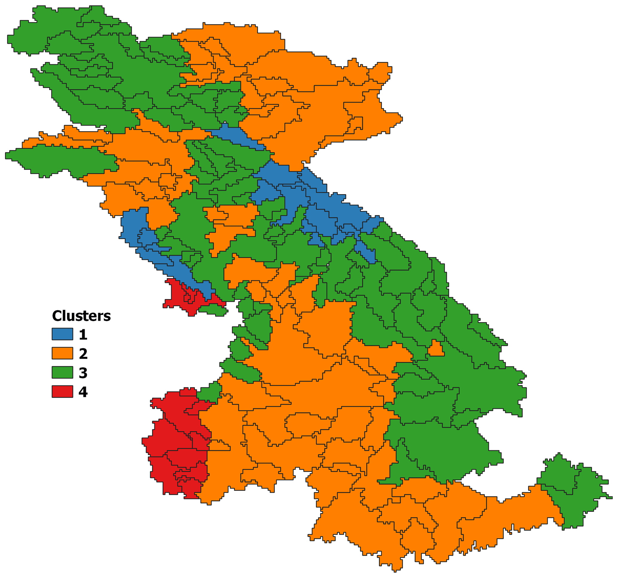
Figure 11 Climatic-based classification of the 158 subbasins of the Peace River, Fraser River and Columbia River basins.

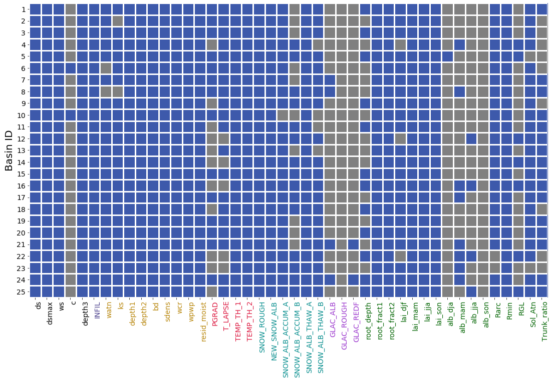
Figure 12 Informative parameters (blue) for at least one of simulated streamflow, evapotranspiration and snow water equivalent. A basin ID description is provided in Table 1.

It has been argued in the literature that calibration based solely on streamflow is not sufficient to ensure model accuracy and fidelity (Rakovec et al., 2016). To improve model realism, recent calibration strategies follow a process-based approach. This approach relies either on adjusting model parameters against hydrological signatures extracted from streamflow time series that link to the underlying model processes (Yilmaz et al., 2008; Euser et al., 2013; Shafii and Tolson, 2015; Rakovec et al., 2016), against measurements of different model outputs such as evapotranspiration, snow cover and baseflow (e.g., Isenstein et al., 2015; Ismail et al., 2020), or on hydrograph decomposition (e.g., He et al., 2015; Shafii et al., 2017; Larabi et al., 2018). However, we recognize that the effort to constrain multiple hydrologic processes will require a substantial increase in the size of the parameter domain during model calibration. For instance, our sensitivity analysis results from Table 5 and Fig. 12 suggest that calibrating VIC-GL in a multi-objective or multi-variable framework would require a high number of parameters in the calibration process (30 to 38 parameters depending on the subbasin if one is to consider all informative parameters for each output considered here). Across the 25 subbasins, an average of 77 % of the parameters (34 of the 44 parameters analyzed) are informative to at least one of simulated streamflow, evapotranspiration or snow water equivalent (see Fig. 12). This contrasts with previous studies that typically calibrate fewer than 12 VIC parameters (e.g., Troy et al., 2008; Isenstein et al., 2015; Mizukami et al., 2017; Rakovec et al., 2019; Ismail et al., 2020). Options to tackle this more complex calibration problem are not evaluated here but could include suitable one-step multi-objective optimization algorithms such as the Pareto Archived Dynamically Dimensioned Search (PA-DDS) (Asadzadeh et al., 2014) or a stepwise multi-objective calibration approach where each set of informative parameters for a specific flux is adjusted separately (Larabi et al., 2018). Another approach to reduce the complexity of the calibration problem would be to use a smaller parameter range, which could speed the convergence rate of the search algorithm to the optimal solution. However, this would have to be done carefully, possibly utilizing expert knowledge, in order to ensure the narrower range still contains the optimal solution (Mai, 2023).

In previous VIC applications, the same parameters are adjusted over large domains to fit the model to streamflow (e.g., Nijssen et al., 2001; Oubeidillah et al., 2014; Xue et al., 2016; Mizukami et al., 2017) and against other model output (Isenstein et al., 2015; Ismail et al., 2020), ignoring both the spatial variability of parameter sensitivity and the dependence of parameter sensitivity on the hydrological processes. To account for this spatial variability, a multi-site cascading approach (Xue et al., 2016) where calibration parameter selection varies depending on the site can be used. Overall, there remains a need to study how information regarding the spatial variability and process dependence of parameter sensitivity is best integrated into a multi-variable parameter estimation framework.

In this study, the low-cost EEE sequential screening method (Cuntz et al., 2105) was used to identify informative parameters. However, this method does not quantitatively rank the importance of these informative parameters. In situations where it is desirable to reduce the number of calibration parameters below the counts identified by EEE analyses, a quantitative approach such as variance-based methods (e.g., Sobol', 1990; Saltelli, 2002) or a qualitative approach that provides parameter groupings based on their sensitivity could be considered (Sheikholeslami et al., 2019; Mai et al., 2020a, 2022). However, future work is required to determine the conditions under which a reduction in the number of calibrated parameters (i.e., by not calibrating some parameters that are informative) could potentially yield better calibration results, particularly in a multi-objective context.

5 Conclusions

Land surface models tend to have large numbers of parameters, many of which cannot be measured directly. Sensitivity analysis is therefore often employed to identify parameters with a significant impact on model output variance. Performing sensitivity analysis for large-scale land surface models is, however, computationally demanding. In this study, we consider whether computational cost can be reduced by using watershed classifications to transfer information on which parameters sensitively affect streamflow, evapotranspiration and snow water equivalent between basins that have similar climatic and vegetation land cover attributes.

The study was performed using a large-domain implementation of a hydrologic model as an example. Specifically, we used an updated version of the VIC model (Schnorbus, 2018) that was coupled to a regional glacier model and implemented across a very large domain in the Pacific Northwest region of North America. A wide range of VIC model parameters was evaluated that includes 5 baseflow parameters, 1 runoff parameter, 9 drainage parameters, 4 climate parameters, 6 snow-related parameters, 3 glacier parameters and 17 vegetation-related parameters. The sensitivity analysis was performed over 25 basins spanning a range of hydroclimatic conditions to understand the spatial variability of parameter sensitivities with regard to streamflow, evapotranspiration and snow water equivalent. Parameter sensitivities for each model output were found to vary in a predictable way with basin climate and land cover characteristics.

Watershed classification was employed to classify the 25 basins into homogenous groups based on climatic attributes (aridity and snow index) and percentage of glacier area and vegetation land cover. This classification was used to transfer sensitive parameters to each basin based on its group membership. This approach was shown to be able to efficiently identify sensitive parameters with median F1 scores of 0.87 for streamflow, 0.83 for evapotranspiration and 0.95 for snow water equivalent. These findings suggest that parameter sensitivity can be performed by classifying watersheds into broad groups and then analyzing sensitivity for only a subset of the basins in each group. In our large domain example, we found that it would likely be sufficient to perform sensitivity analysis in 4 % (or fewer) of the basins contained within the domain. This would substantially reduce the cost of the sensitivity analyses that are used to determine the model calibration strategy or, for a given computing budget, would enable the consideration of a broader range of parameters than could be considered if a sensitivity analysis were to be performed across the entire domain.

The parameter classification based on parameter sensitivities informs which parameters should be adjusted (invariant-informative and variant-informative) depending on the calibration variables that are considered and the local climatic conditions. We found that, for a multi-variable calibration approach targeting streamflow, evapotranspiration and snow water equivalent, an average of 77 % of the VIC parameters (i.e., 34 of the 44 parameters analyzed) were identified as calibration candidates. These parameters include not only those that control runoff and baseflow generation, but also parameters that control snow processes and describe vegetation properties. The findings of this study highlight the need to explore efficient ways of decreasing the complexity of multi-process-based calibration of land surface models arising from the increased dimensionality of both the parameter and objective function spaces.

Finally, we note that more specific modeling objectives, such as the skillful representation of peak flows (for flood forecasting purposes) or low flows (for predicting summer drought impacts), could also be considered using the approach that has been proposed. Similarly, the results and methods are applicable to other land surface models.