Flow recession behavior of preferential subsurface flow patterns with minimum energy dissipation

Understanding the properties of preferential flow patterns is a major challenge in subsurface hydrology. Most of the theoretical approaches in this field stem from research on karst aquifers, where two or three distinct flow components with different timescales are typically considered. This study is based on a different concept: a continuous spatial variation in transmissivity and storativity over several orders of magnitude is assumed. The distribution and spatial pattern of these properties are derived from the concept of minimum energy dissipation. While the numerical simulation of such systems is challenging, it is found that a restriction to a dendritic flow pattern, similar to rivers at the surface, works well. It is also shown that spectral theory is useful for investigating the fundamental properties of such aquifers. As a main result, the long-term recession of the spring draining the aquifer during periods of drought becomes slower for large catchments. However, the dependence of the respective recession coefficient on catchment size is much weaker than for homogeneous aquifers. Concerning the short-term behavior after an instantaneous recharge event, strong deviations from the exponential recession of a linear reservoir are observed. In particular, it takes a considerable time span until the spring discharge reaches its peak. The order of magnitude of this rise time is one-seventh of the characteristic time of the aquifer. Despite the strong deviations from the linear reservoir at short time spans, the exponential component typically contributes more than 80 % to the total discharge. This fraction is much higher than expected for karst aquifers and even exceeds the fraction predicted for homogeneous aquifers.

1 Introduction

The recession of spring discharge after recharge events can be seen as the fingerprint of an aquifer. In contrast to pumping tests at wells, it is a passive method based on data that are often recorded routinely. Additionally, spring discharges depend on the overall properties of the catchment, whereas pumping tests reflect the properties in a region around the well.

More than a century ago, Maillet (1905) proposed the linear reservoir, where discharge Q is directly proportional to the stored volume V:

$$\begin{array}{}\text{(1)}& Q\left(t\right)=\mathit{\alpha }V\left(t\right).\end{array}$$

The linear reservoir is described by a single parameter α (s⁻¹), and the stored volume follows the ordinary differential equation:

$$\begin{array}{}\text{(2)}& {\displaystyle \frac{\mathrm{d}}{\mathrm{d}t}}V\left(t\right)=-Q\left(t\right)+R\left(t\right)=-\mathit{\alpha }V\left(t\right)+R\left(t\right),\end{array}$$

where R(t) (m³ s⁻¹) is the recharge. During periods with zero recharge, both the stored volume and the discharge decay exponentially with the same decay constant α, also called the recession coefficient:

$$\begin{array}{}\text{(3)}& {\displaystyle }& {\displaystyle }V\left(t\right)=V\left(\mathrm{0}\right)e^{-\mathit{\alpha }t},\text{(4)}& {\displaystyle }& {\displaystyle }Q\left(t\right)=Q\left(\mathrm{0}\right)e^{-\mathit{\alpha }t}.\end{array}$$

The inverse of the recession coefficient, $\mathit{\tau }=\frac{\mathrm{1}}{\mathit{\alpha }}$, defines the e-folding time: the time interval over which the discharge decreases by a factor of e.

The linear reservoir is not only appealing because it can be described by a single parameter but also because its behavior during periods of drought depends only on the actual amount of water and is independent of the recharge history. It often provides a reasonable approximation for long periods of drought. Deviations from the exponential decay at shorter timescales have been investigated and used for characterizing aquifers since the 1960s; in particular, karst systems have been addressed in numerous studies, and several theoretical concepts have been proposed.

Forkasiewicz and Paloc (1967) suggested a superposition of three distinct linear reservoirs with different decay constants describing three major flow components: a network of highly conductive conduits, an intermediate system of well integrated fissures, and a network of pores or narrow fissures with low permeability. The behavior of this model is dominated by the slowest reservoir during long periods of drought.

Mangin (1975) introduced a different approach using two components. The slow component was described as a linear reservoir, and a fast component with a limited range was added. The parameters of the fast components are the basis of the widely used karst classification system suggested in the same study. Several other modeling approaches which are similar in spirit were developed (e.g., Drogue, 1972; Atkinson, 1977; Padilla et al., 1994; Kovács and Perrochet, 2014; Xu et al., 2018; Basha, 2020; Kovács, 2021). Beyond these approaches, a multitude of numerical models designed for simulating real-world scenarios are now available. For deeper insights, readers are referred to the review paper by Fiorillo (2014) and to the model comparison by Jeannin et al. (2021).

While deviations from the linear reservoir are particularly relevant for karst systems, it should be noted that even the simplest Darcy-type aquifers are not linear reservoirs. Assuming a given transmissivity T (m² s⁻¹) and a given storativity S (–), the simplest Darcy-type aquifer is described by the water balance equation:

$$\begin{array}{}\text{(5)}& S{\displaystyle \frac{\partial h}{\partial t}}=-\mathrm{div}\mathit{q}+r,\end{array}$$

where h (m) is the hydraulic head,

$$\begin{array}{}\text{(6)}& \mathit{q}=-T\mathrm{\nabla }h\end{array}$$

(m² s⁻¹) is the 2-D flux density (volume per time and cross-section width), ∇ is the 2-D gradient operator, r is the recharge per area (ms⁻¹), and div is the 2-D divergence operator. Inserting Eq. (6) into Eq. (5) yields a partial differential equation of the diffusion type for the hydraulic head h:

$$\begin{array}{}\text{(7)}& S{\displaystyle \frac{\partial h}{\partial t}}=\mathrm{div}\left(T\mathrm{\nabla }h\right)+r.\end{array}$$

This model has been investigated in several studies for constant T and S in square or rectangular domains (e.g., Rorabaugh, 1964; Nutbrown, 1975; Kovács et al., 2005; Kovács and Perrochet, 2008). Applying spectral theory (see Sect. 2.4), it has been shown that the total discharge Q (q integrated over the entire boundary) can be described by an infinite series of exponential terms with different decay constants during periods of drought. As the long-term recession is dominated by the term with the smallest decay constant, the behavior approaches that of the linear reservoir. However, the question of how well the linear reservoir approximates the properties of real aquifers in a practical sense or whether the linear reservoir is even some kind of preferred state from a theoretical point of view has prompted debate (e.g., Fenicia et al., 2006; de Rooij, 2014; Kleidon and Savenije, 2017; Savenije, 2018).

Including the early recession phase in the analysis yields more information about the aquifer but also increases the dependence of the results on the recharge history. The instantaneous unit hydrograph, which dates back to concepts of Sherman (1932), is widely used in this context. It describes the discharge arising from a unit amount of recharge that is applied instantaneously at t=0 over the entire domain.

The unit hydrograph of the simple Darcy aquifer differs strongly from that of the linear reservoir as well as from the empirical approaches proposed by Forkasiewicz and Paloc (1967) and by Mangin (1975). While these models predict a finite discharge at t=0, the unit hydrograph diverges according to a power law,

$$\begin{array}{}\text{(8)}& Q\left(t\right)\propto t^{-\frac{\mathrm{1}}{\mathrm{2}}},\end{array}$$

in the limit t→0 for the simple Darcy aquifer (e.g., Hergarten and Birk, 2007). Such a power-law decrease also occurs in models consisting of porous blocks connected by highly conductive conduits (Kovács et al., 2005; Kovács and Perrochet, 2008). However, a finite conductance of the conduits limits the power-law divergence at short timescales (Kovács and Perrochet, 2014). Hergarten and Birk (2007) extended this concept using a fractal distribution of block sizes. While this model was able to explain a power-law recession with exponents different from $-\frac{\mathrm{1}}{\mathrm{2}}$, deriving aquifer properties from the power-law behavior of recession curves turned out to be challenging. Birk and Hergarten (2010) investigated synthetic hydrographs for recharge events of finite duration and found that the properties of the recharge event likely obscure the short-term dynamics of the porous blocks.

The quantification of heterogeneity and its representation in numerical models are still major challenges in hydrology. Carbonatic aquifers are particularly interesting in this context due to the interplay between fluid flow and structure. The spatial structure of the aquifer has a strong influence on fluid flow, which in turn controls dissolution and precipitation and, thus, the long-term change in the large-scale structure. This interaction has been addressed in modeling studies of binary karst systems consisting of a porous medium and discrete conduits (e.g., Kaufmann and Braun, 2000; Kaufmann et al., 2010; Birk et al., 2003) as well as in the context of continuous changes in porosity and conductivity (e.g., Edery et al., 2021). Similar processes can also take place in soils by subsurface erosion (e.g., Bernatek-Jakiel and Poesen, 2018).

As an alternative to forward modeling, there is an increasing number of studies attempting to derive preferred states of the atmosphere and the hydrosphere from principles of optimality (e.g., Kleidon and Schymanski, 2008; Kleidon and Renner, 2013; Kleidon et al., 2014; Kleidon and Savenije, 2017; Kleidon et al., 2019; Zehe et al., 2010, 2013, 2021; Westhoff and Zehe, 2013; Westhoff et al., 2014, 2017; Zhao et al., 2016; Schroers et al., 2022). In the context of fluid flow, minimum energy dissipation seems to be a promising concept, and it has been successfully applied to river networks (Howard, 1990; Rodriguez-Iturbe et al., 1992a, b; Rinaldo et al., 1992; Maritan et al., 1996) and to the cardiovascular system of mammals (West et al., 1997; Enquist et al., 1998, 1999; Banavar et al., 1999; West et al., 1999a, b).

Hergarten et al. (2014) developed a theory for an optimal spatial distribution of porosity and hydraulic conductivity in the sense that the total energy dissipation of the flow is minimized. A major difference from the studies focusing on karst systems mentioned above is that this theory does not predict a binary or ternary system of distinct flow components but rather a continuous variation in the hydraulic properties over several orders of magnitude in combination with a highly organized spatial pattern. The predicted spatial pattern is dendritic and similar to drainage networks at the surface. Therefore, it does not entirely capture the variety of preferential flow patterns found in nature.

The potential relation of this theoretical concept to subsurface hydrology is still unclear. Validation is limited to the statistical distribution of catchment sizes and leaves several open questions (Hergarten et al., 2016). Even the properties of the model have not been analyzed thoroughly, except for residence times in a steady state (Hergarten et al., 2014).

This study investigates the dynamic properties of such preferential flow patterns based on the instantaneous unit hydrograph. The main research question is how preferential flow patterns with minimum energy dissipation are related to the different concepts discussed above. However, we also pose the following more detailed research questions:

• How much does the behavior of preferential flow patterns differ from that of a homogeneous aquifer or a linear reservoir?

• Can we explain the typical behavior of karst springs without assuming two or three distinct flow components?

• Which physical properties do short- and long-term properties of such an aquifer depend on?

2 Approach

2.1 Linearized consideration

The instantaneous unit hydrograph describes the response of an aquifer to adding a unit amount of water instantaneously. It is particularly useful for linear systems because the response to any recharge curve r(t) can be obtained by superposing multiple recharge events at different times (formally, the convolution integral of r(t) and the instantaneous unit hydrograph).

For unconfined aquifers, however, the transmissivity is proportional to the height of the water column:

$$\begin{array}{}\text{(9)}& T=K(h-b),\end{array}$$

where K is the hydraulic conductivity (m s⁻¹) and b is the base of the aquifer (m). As this dependence introduces a nonlinearity in Eq. (7), we can only make use of the linear theory for small disturbances. For this, we assume a steady state at a recharge r₀ and apply a small additional recharge δr, so that $r=r_{\mathrm{0}}+\mathit{\delta }r$. We can then write the actual head in the form $h=h_{\mathrm{0}}+\mathit{\delta }h$ with the steady-state head h₀. Equation (5) retains its shape,

$$\begin{array}{}\text{(10)}& S{\displaystyle \frac{\partial \mathit{\delta }h}{\partial t}}=-\mathrm{div}\mathit{\delta }\mathit{q}+\mathit{\delta }r,\end{array}$$

but with

$$\begin{array}{}\text{(11)}& {\displaystyle }\mathit{\delta }\mathit{q}& {\displaystyle }=-K\left(\left(h_{\mathrm{0}}+\mathit{\delta }h-b\right)\mathrm{\nabla }\left(h_{\mathrm{0}}+\mathit{\delta }h\right)+\left(h_{\mathrm{0}}-b\right)\mathrm{\nabla }{h}_{\mathrm{0}}\right)\text{(12)}& {\displaystyle }& {\displaystyle }\approx -K\left(\left(h_{\mathrm{0}}-b\right)\mathrm{\nabla }\mathit{\delta }h+\mathit{\delta }h\mathrm{\nabla }{h}_{\mathrm{0}}\right)\end{array}$$

for small δh. The first term is the effect of a change in the hydraulic gradient at constant transmissivity $T_{\mathrm{0}}=K(h_{\mathrm{0}}-b)$, which has the same form as Eq. (6). The second term describes the change in flux arising from the change in the thickness of the water column at constant hydraulic gradient. This term is particularly relevant for sloping aquifers with thin water layers.

As the concept developed in the following only captures the first term, the second term is neglected in this study. This means that the steady-state water table should be almost horizontal and the respective water column should not be too thin. In this case (neglecting the second term in Eq. 12), δh is described by the same equation as h in Eq. (7) but with δr and T=T₀. For simplicity, δh, δq, and δr are labeled h, q, and r, respectively. Thus, we have to keep in mind that these properties are not absolute values but rather small deviations from a steady state. Furthermore, T is the steady-state transmissivity T₀ in the following.

2.2 Basic setup

Following the considerations outlined in the previous section, we consider a 2-D aquifer with a given transmissivity T (m² s⁻¹) and a given storativity S (–), described by Eqs. (5) and (6). As the focus is on strongly organized preferential flow patterns, both T and S are not spatially uniform and may even vary over several orders of magnitude. As discussed in the previous section, the head values h, the flux density q, and the recharge r are not absolute values but rather deviations from a steady state. As the simplest boundary condition, it can be assumed that the hydraulic head at springs remains constant, which is equivalent to the boundary condition h=0.

On a regular grid with a uniform grid spacing d, Eqs. (5) and (6) can be discretized by a finite-volume approach according to

$$\begin{array}{}\text{(13)}& d^{\mathrm{2}}{S}_i{\displaystyle \frac{\partial h_i}{\partial t}}=-\sum _{j\in N\left(i\right)}{q}_{ij}+d^{\mathrm{2}}{r}_i\end{array}$$

with the fluxes

$$\begin{array}{}\text{(14)}& q_{ij}=d{T}_{ij}{\displaystyle \frac{h_i-h_j}{d}}.\end{array}$$

The nodes of the grid were numbered by a single index i, where N(i) denotes the nearest neighborhood of the node i, consisting of four neighbors except for boundary nodes. The symbol q_ij (m² s⁻¹) refers to the flux from the node i to the node j, while T_ij is the respective transmissivity. Note that q_ij already includes the length of the edge between the two nodes (first term d in Eq. 14), so that it is no longer a flux per unit width. Inserting Eq. (14) into Eq. (13) yields the respective discrete form of Eq. (7).

Solving this equation numerically on large grids is challenging if the transmissivity varies over several orders of magnitude. Using an explicit scheme for the time step requires very small time increments because small changes in hydraulic head cause large fluxes. Employing a fully implicit scheme overcomes this limitation, as fully implicit schemes are stable at arbitrary time increments for diffusion-type equations. However, most of the available algorithms for solving the resulting linear equation system do not perform well if T varies strongly. This also applies to multigrid schemes (e.g., Hackbusch, 1985), which are the only schemes with a numerical effort that increases only linearly with the number of nodes.

2.3 Dendritic flow patterns

The theory of minimum energy dissipation in Darcy flow proposed by Hergarten et al. (2014) approximates preferential flow patterns by dendritic structures. This means that each node i delivers its entire discharge to one of its neighbors, b, referred to as the flow target in the following (strictly speaking, it should be labeled b_i). The flow target is defined as the neighbor with the steepest descent in hydraulic head, which is the same as the neighbor with the lowest head value for a grid with uniform spacing in both directions. Then, the neighborhood consists of three groups of nodes: (i) one flow target; (ii) some neighbors that deliver their discharge to the considered node, called donors in the following; and (iii) some nodes that do not interact with the considered node. The last group of nodes results in the difference from the original model where all neighboring nodes interact.

As we consider only small deviations from a steady state, we can assume that the topology of the flow pattern does not change through time. The flow target of each node is determined from the steady state and persists. As a major advantage, this simplification inhibits the occurrence of nodes without a flow target.

The discrete version of the balance equation (Eq. 13) becomes

$$\begin{array}{}\text{(15)}& d^{\mathrm{2}}{S}_i{\displaystyle \frac{\partial h_i}{\partial t}}=-q_i+\sum _{j\in D\left(i\right)}{q}_j+d^{\mathrm{2}}{r}_i\end{array}$$

for a dendritic flow pattern, where the notation q_i (with a single index) describes the flux from the node i to its flow target (so q_ib in the general notation). The sum extends over all donors of the node i, denoted here as D(i).

Because the topology of the flow pattern is static, the head value of a node may become lower than that of its flow target, in which case Eq. (14) predicts a negative flux. In the context of small deviations from a steady state, a negative flux would not have an immediate meaning because it just says that the flux towards the flow target is lower than in the steady state. However, there is no problem, even if backward flux occurs on an absolute scale.

Dendritic networks are widely used in the context of surface flow patterns, in particular river networks at large scales. In order to reduce the effects of anisotropy, the so-called D8 scheme is typically used on a regular, 2-D grid. Here, eight neighbors (four nearest neighbors and four diagonal neighbors) are considered, so that river segments are either parallel to one of the coordinate axes or diagonal. While the numerical construction of optimized drainage patterns by Hergarten et al. (2014) also used the D8 scheme, we consider only the four nearest neighbors (D4 scheme) in the following. The main reason for this limitation is the comparison to the original model in Sect. 3.1. The D4 scheme can be seen as a restriction of the original model, whereas the D8 version would allow for additional flow paths. In particular, a diagonal line of points with a high transmissivity would be a preferential flow path with regard to the D8 scheme, although not in the original model.

While the concept of dendritic flow patterns was used by Hergarten et al. (2014) to construct patterns of porosity and conductivity (see also Sect. 2.7), recent developments in numerics make this concept interesting for time-dependent modeling. In the following sections, two numerical approaches that are robust against strong variations in transmissivity are presented.

2.4 Spectral theory

Large parts of this study are based on spectral theory. Spectral theory decomposes the solution into a set of functions with a simple behavior. The functions are simple in the sense that they can be written in the form

$$\begin{array}{}\text{(16)}& h(\mathit{x},t)=h(\mathit{x},\mathrm{0})f\left(t\right),\end{array}$$

which means that their shape does not change through time. For r=0, Eq. (7) can then be separated into one equation for h(x,0) and another equation for the time dependence f(t). This result is recognized by inserting h(x,t) into Eq. (7) and dividing both sides by h(x,t) and by S, which yields

$$\begin{array}{}\text{(17)}& {\displaystyle \frac{\frac{\mathrm{d}}{\mathrm{d}t}f\left(t\right)}{f\left(t\right)}}={\displaystyle \frac{\frac{\mathrm{1}}{S}\mathrm{div}\left(T\mathrm{\nabla }h\right(\mathit{x},\mathrm{0}\left)\right)}{h(\mathit{x},\mathrm{0})}}.\end{array}$$

As the left-hand side is independent of x and the right-hand side is independent of t, both sides must be constant. If we call the respective constant −α, the solution for f is

$$\begin{array}{}\text{(18)}& f\left(t\right)=e^{-\mathit{\alpha }t}\end{array}$$

because Eq. (16) requires f(0)=1. Thus,

$$\begin{array}{}\text{(19)}& h(\mathit{x},t)=h(\mathit{x},\mathrm{0})e^{-\mathit{\alpha }t}\end{array}$$

decreases exponentially for α>0 and increases for α<0. The right-hand side of Eq. (17) yields the eigenvalue equation

$$\begin{array}{}\text{(20)}& -{\displaystyle \frac{\mathrm{1}}{S}}\mathrm{div}\left(T\mathrm{\nabla }h\right)=\mathit{\alpha }h\end{array}$$

for h(x,0). This means that the differential operator $-\frac{\mathrm{1}}{S}\mathrm{div}T\mathrm{\nabla }$ applied to the function h just multiplies h by the factor α. Mathematically, h is an eigenfunction of the differential operator and α is the respective eigenvalue.

While the eigenfunctions and the respective eigenvalues can be computed analytically for some simple geometries (e.g., Rorabaugh, 1964; Nutbrown, 1975; Kovács et al., 2005; Kovács and Perrochet, 2008) and constant parameters, a heterogeneous distribution of S and T requires a numerical treatment. The numerical treatment requires a transition from the continuous function h to the values h_i on the discrete grid. Using the same finite-volume discretization as above (Eqs. 13 and 14), the term $-\frac{\mathrm{1}}{S}\mathrm{div}\left(T\mathrm{\nabla }h\right)$ can be approximated at the ith node by

$$\begin{array}{}\text{(21)}& {\left.-{\displaystyle \frac{\mathrm{1}}{S}}\mathrm{div}\left(T\mathrm{\nabla }h\right)\right|}_i\approx {\displaystyle \frac{\mathrm{1}}{S_i}}\sum _{j\in N\left(i\right)}{T}_{ij}\left(h_i-h_j\right),\end{array}$$

where unit grid spacing (d=1) was assumed for simplicity. Aligning all values h_i in a column vector h, this relation can be written in matrix form

$$\begin{array}{}\text{(22)}& -{\displaystyle \frac{\mathrm{1}}{S}}\mathrm{div}\left(T\mathrm{\nabla }h\right)\approx \mathbf{A}\mathit{h}\end{array}$$

with a square matrix A. It is easily recognized that the non-diagonal elements of A are

$$\begin{array}{}\text{(23)}& A_{ij}=\left\{\begin{array}{ll}-\frac{T_{ij}}{S_i}& \mathrm{for}j\in N\left(i\right)\\ \mathrm{0}& \mathrm{else}\end{array}\right.,\end{array}$$

whereas the diagonal elements are

$$\begin{array}{}\text{(24)}& A_{ii}=\sum _{j\in N\left(i\right)}\left(-A_{ij}\right)=\sum _{j\in N\left(i\right)}{\displaystyle \frac{T_{ij}}{S_i}}.\end{array}$$

This matrix is the same as that needed for solving the steady-state version of Eq. (7) numerically. The respective form of the matrix for dendritic flow patterns is basically the same, where only the neighborhood has to be reduced to those points that are connected, i.e., where either j is the flow target of i or vice versa.

As all software packages for linear algebra provide functions for computing eigenvalues, the steps are technically not very challenging up to this point. However, each eigenvalue and the respective eigenfunction is just one solution of Eq. (7) with r=0 for a specific initial condition h(x,0). In turn, we need the solution for any given initial condition. Spectral theory expresses a given initial condition as a superposition of eigenfunctions and then uses the knowledge about the individual eigenfunctions for predicting the full solution.

Let us assume that we computed all eigenfunctions and that e_ki is the value of the kth eigenfunction at the node i. If h_i(0) is the initial value at this node, we need coefficients λ_k so that h_i(0) is the superposition of the respective values e_ki,

$$\begin{array}{}\text{(25)}& h_i\left(\mathrm{0}\right)=\sum _k{\mathit{\lambda }}_k{e}_{ki}.\end{array}$$

Then, the values of h at time t are

$$\begin{array}{}\text{(26)}& h_i\left(t\right)=\sum _k{\mathit{\lambda }}_k{e}_{ki}{e}^{-{\mathit{\alpha }}_{k}t},\end{array}$$

where α_k is the kth eigenvalue of A. Thus, all head values can be written as a sum of exponentially decaying terms, provided that all eigenvalues are positive. The latter can be shown for the matrix defined by Eqs. (23) and (24) with the help of Gershgorin's circle theorem.

Because all head values can be decomposed into a sum of exponential functions, the fluxes and, thus, the discharge of a spring can be expressed the same way:

$$\begin{array}{}\text{(27)}& Q\left(t\right)=\sum _k{\mathit{\lambda }}_k{Q}_k{e}^{-{\mathit{\alpha }}_{k}t},\end{array}$$

where Q_k is the discharge of the kth eigenfunction. If we assume that the eigenvalues are sorted in increasing order, the long-term recession coefficient is α=α₁.

The nontrivial question is whether each initial condition can be expressed as a superposition of eigenfunctions according to Eq. (25). Mathematically, this property relies on the symmetry of the differential operator or, for the discrete problem, on the symmetry of the matrix (A_ij=A_ji). If A is symmetric, a basis of eigenvectors (the representations of the eigenfunctions on the discrete grid) can be found, which ensures the applicability of Eq. (25) for any initial condition with unique coefficients λ_k.

The symmetry of A even guarantees the existence of an orthonormal basis. As a main advantage, an orthonormal basis allows for the computation of each coefficient λ_k from the inner product (scalar product) of the initial head distribution and the respective eigenvector. Therefore, we can obtain the long-term recession coefficient α=α₁ and the contribution of the respective component to the total (time-integrated) discharge from the lowest eigenvalue and the respective eigenvector alone. Otherwise, we would need all eigenvectors. As their number equals the number of nodes, this would be expensive on large grids and would cost the advantage over a direct forward simulation.

Because T_ij is the transmissivity between the nodes i and j, T_ij=T_ji. Without the term S_i in Eq. (23), this property would already guarantee the symmetry of A. With this term, however, A is only symmetric if S_i=S_j, i.e., if S is the same everywhere.

To overcome this limitation, we need to get a bit deeper into linear algebra and consider a wider definition of symmetry coming from the concept of linear maps. Here, symmetry is related to an inner product, and the condition for symmetry is

$$\begin{array}{}\text{(28)}& \mathbf{A}\mathit{h}\cdot \stackrel{\mathrm{̃}}{\mathit{h}}=\mathit{h}\cdot \mathbf{A}\stackrel{\mathrm{̃}}{\mathit{h}},\end{array}$$

where ⋅ is the inner product. This condition has to be satisfied for all h and $\stackrel{\mathrm{̃}}{\mathit{h}}$. It is easily recognized that the criterion A_ij=A_ji describes the specific case for the standard scalar product

$$\begin{array}{}\text{(29)}& \mathit{h}\cdot \stackrel{\mathrm{̃}}{\mathit{h}}=\sum _i{h}_i{\stackrel{\mathrm{̃}}{h}}_i.\end{array}$$

For deeper insights into the fundamentals, readers are referred to textbooks of linear algebra (e.g., Halmos, 1958).

To examine the symmetry of A in this sense, we need the custom inner product

$$\begin{array}{}\text{(30)}& \mathit{h}\cdot \stackrel{\mathrm{̃}}{\mathit{h}}=\sum _i{S}_i{h}_i{\stackrel{\mathrm{̃}}{h}}_i,\end{array}$$

which differs from the standard scalar product (Eq. 29) by its weighting with the storativity S. Using the definition of A (Eqs. 23 and 24), it is easily recognized that

$$\begin{array}{}\text{(31)}& S_i{A}_{ij}=S_j{A}_{ji},\end{array}$$

and thus

$$\begin{array}{}\text{(32)}& \left(\mathbf{A}\mathit{h}\right)\cdot \stackrel{\mathrm{̃}}{\mathit{h}}=\sum _i{S}_i\left(\sum _j{A}_{ij}{h}_j\right){\stackrel{\mathrm{̃}}{h}}_i\end{array}$$

$$\begin{array}{}\text{(33)}& {\displaystyle }& {\displaystyle }=\sum _{i,j}{S}_i{A}_{ij}{h}_j{\stackrel{\mathrm{̃}}{h}}_i\text{(34)}& {\displaystyle }& {\displaystyle }=\sum _{i,j}{S}_j{A}_{ji}{h}_j{\stackrel{\mathrm{̃}}{h}}_i\text{(35)}& {\displaystyle }& {\displaystyle }=\sum _{i,j}{S}_j{h}_j\left(\sum _i{A}_{ji}{\stackrel{\mathrm{̃}}{h}}_i\right)\text{(36)}& {\displaystyle }& {\displaystyle }=\mathit{h}\cdot \left(\mathbf{A}\stackrel{\mathrm{̃}}{\mathit{h}}\right),\end{array}$$

which proves the symmetry of A with regard to the custom inner product.

Technically, the normalization of the eigenvectors obtained numerically is the only point that requires attention. The eigenvectors have to be normalized with respect to the custom inner product and not with respect to the standard scalar product, i.e., according to the condition

$$\begin{array}{}\text{(37)}& {\mathit{e}}_k\cdot {\mathit{e}}_k=\sum _i{S}_i{e}_{ki}^{\mathrm{2}}=\mathrm{1}.\end{array}$$

If h_i represents the head values at t=0, the coefficients λ_k in Eqs. (25) and (26) are then obtained from the inner products in the following form:

$$\begin{array}{}\text{(38)}& {\mathit{\lambda }}_k=\mathit{h}\cdot {\mathit{e}}_k=\sum _i{S}_i{h}_i{e}_{ki}.\end{array}$$

This relation becomes particularly simple for the instantaneous unit hydrograph. Applying a unit amount of water per area to all nodes results in S_ih_i=1 for all i, and thus

$$\begin{array}{}\text{(39)}& {\mathit{\lambda }}_k=\sum _i{e}_{ki}.\end{array}$$

Thus, the coefficient λ_k is obtained by adding the head values of the respective normalized eigenfunction at all nodes.

2.5 Forward modeling

Spectral theory is very efficient for characterizing the long-term recession, as only the components with the lowest recession coefficients α_k are relevant here. In turn, computing the instantaneous unit hydrograph at short timescales requires a large number of eigenfunctions, so that the advantage over direct forward modeling is lost. Therefore, we also implemented a numerical scheme for forward modeling of the dendritic model. For this purpose, we adopted the very efficient, fully implicit scheme that was recently proposed in the context of fluvial erosion and sediment transport by Hergarten (2020). As a major advantage, the scheme is robust against strong spatial variations in transmissivity. For simplicity, the scheme is only described for the D4 neighborhood with unit grid spacing (d=1) in the following.

Let us consider a time step from t to t+δt. Replacing the time derivative on the left-hand side of Eq. (15) with a difference quotient and evaluating the fluxes on the right-hand side at the time t+δt (for the fully implicit treatment) yields

$$\begin{array}{}\text{(40)}& S_i{\displaystyle \frac{h_i(t+\mathit{\delta }t)-h_i\left(t\right)}{\mathit{\delta }t}}=-q_i(t+\mathit{\delta }t)+\sum _{j\in D\left(i\right)}{q}_j(t+\mathit{\delta }t)+r_i.\end{array}$$

The key idea behind the scheme is that all fluxes respond linearly to changes in h of the flow target b due to the linearity of the differential equation. In particular, the flux q_i(t+δt) depends linearly on h_b, so that

$$\begin{array}{}\text{(41)}& q_i(t+\mathit{\delta }t)=q_i^{\mathrm{0}}+q_i^{\prime }\left(h_b(t+\mathit{\delta }t)-h_b\left(t\right)\right).\end{array}$$

Here, $q_i^{\mathrm{0}}$ is the hypothetic flux at time t+δt under the assumption that h_b remains constant ($h_b(t+\mathit{\delta }t)=h_b\left(t\right)$). It is not the same as q_i(t) because q_i may also change if q_b remains constant. The second term in Eq. (41) describes the effect of changes in h_b(t+δt) on q_i(t+δt), where $q_i^{\prime }$ is the partial derivative of q_i(t+δt) with respect to h_b(t+δt).

As shown in Appendix A, $q_i^{\mathrm{0}}$ and $q_i^{\prime }$ can be computed from the respective properties of the donors and from the known values of h at time t by the following expressions:

$$\begin{array}{}\text{(42)}& {\displaystyle }& {\displaystyle }{q}_i^{\mathrm{0}}=T_i{\displaystyle \frac{\left(\frac{S_i}{\mathit{\delta }t}-\sum _j{q}_j^{\prime }\right)\left(h_i\left(t\right)-h_b\left(t\right)\right)+\sum _j{q}_j^{\mathrm{0}}+r_i}{\frac{S_i}{\mathit{\delta }t}+T_i-\sum _j{q}_j^{\prime }}},\text{(43)}& {\displaystyle }& {\displaystyle }{q}_i^{\prime }=-T_i{\displaystyle \frac{\frac{S_i}{\mathit{\delta }t}-\sum _j{q}_j^{\prime }}{\frac{S_i}{\mathit{\delta }t}+T_i-\sum _j{q}_j^{\prime }}}.\end{array}$$

Thus, $q_i^{\mathrm{0}}$ and $q_i^{\prime }$ can be computed successively in downstream order, starting from the nodes without donors.

However, q_i(t+δt) cannot be computed during the downstream sweep because the actual values h_b(t+δt) required in Eq. (41) are still unknown. Computing the values h_i(t+δt) and q_i(t+δt) requires a second sweep over all nodes, which has to be performed in the opposite direction (upstream, starting from the boundary). As soon as h_b(t+δt) is known (as the node b is treated prior to the node i), q_i(t+δt) can be computed from Eq. (41). Finally, the hydraulic head can be calculated from Eq. (14) according to

$$\begin{array}{}\text{(44)}& h_i(t+\mathit{\delta }t)=h_b(t+\mathit{\delta }t)+{\displaystyle \frac{q_i(t+\mathit{\delta }t)}{T_i}}.\end{array}$$

This scheme provides a direct solver (without the need for iterations) for the fully implicit discretization of the flow equation on a dendritic network. As mentioned at the end of Sect. 2.2, fully implicit schemes are stable for arbitrary time increments δt. As a main advantage over other efficient schemes (e.g., multigrid schemes), the performance of this scheme is not affected by spatial variations in transmissivity and storativity. The numerical complexity is O(n), which means that the computing effort increases only linearly with the total number of nodes. It is, therefore, perfectly suited for simulations on grids with several million nodes.

2.6 Nondimensionalization

The linearized problem (Eq. 7, where T does not depend on h) can easily be transformed to nondimensional properties, which makes the results independent of the absolute values of S and T and of the spatial scale. For this purpose, arbitrary reference values S₀ and T₀ and an arbitrary length scale l can be defined. Then, the respective nondimensional properties

$$\begin{array}{}\text{(45)}& \widehat{S}={\displaystyle \frac{S}{S_{\mathrm{0}}}},\widehat{T}={\displaystyle \frac{T}{T_{\mathrm{0}}}},\mathrm{and}\widehat{x}={\displaystyle \frac{x}{l}}\end{array}$$

are defined. If we further introduce

$$\begin{array}{}\text{(46)}& t_{\mathrm{0}}={\displaystyle \frac{S_{\mathrm{0}}{l}^{\mathrm{2}}}{T_{\mathrm{0}}}}\mathrm{and}{r}_{\mathrm{0}}={\displaystyle \frac{T_{\mathrm{0}}}{l}}\end{array}$$

and define the nondimensional properties

$$\begin{array}{}\text{(47)}& \widehat{h}={\displaystyle \frac{h}{l}},\widehat{t}={\displaystyle \frac{t}{t_{\mathrm{0}}}},\mathrm{and}\widehat{r}={\displaystyle \frac{r}{r_{\mathrm{0}}}},\end{array}$$

the differential equation for the nondimensional properties is the same as the original equation (Eq. 7). This result can easily be verified by expressing the original properties in Eq. (7) in terms of the respective nondimensional properties. The scaling factor for the flux density is T₀ then, so $\mathit{q}=T_{\mathrm{0}}\widehat{\mathit{q}}$.

As a consequence of these scaling properties, the shape of the instantaneous unit hydrograph depends only on the shape of the aquifer and on the spatial pattern of S and T. It is independent of the absolute values of S and T and on the absolute size of the aquifer. This property will become useful in the following section.

2.7 Patterns of transmissivity and storativity

While systematic knowledge about the spatial structure of preferential flow paths is still limited, we need a model for generating spatial patterns of transmissivity and storativity. In this study, we adopt the theory based on minimum energy dissipation proposed by Hergarten et al. (2014). This theory addresses the best spatial distribution of a given total pore space volume in the sense that the total energy dissipation of steady-state flow is minimized. The central assumption behind this theory is a power-law relation between the hydraulic conductivity K on the porosity ϕ,

$$\begin{array}{}\text{(48)}& K\propto {\mathit{\varphi }}^n,\end{array}$$

with a given exponent n. Some ideas regarding how dissolution could increase K were discussed in the aforementioned study. If all pores have the same diameter and grow uniformly, an exponent n=2 was obtained. The same result was obtained for an arbitrary distribution of diameters if all pores grow by the same factor with respect to diameter. In turn, a stronger increase in K with ϕ (n>2) occurs if dissolution mainly affects the largest pores. Overall, these simple models yield a weaker increase in conductivity with porosity than predicted by the fundamental relation of Kozeny (1927) and Carman (1937). This relation predicts n=3 at small porosities, which was also adopted in the numerical study of dissolution and precipitation by Edery et al. (2021). In turn, the theoretical study of fractal pore spaces by Costa (2006) points towards n≈2.

The exact value of the exponent n is, however, not important in the following. Theoretically, it is only important that the increase in K with ϕ is stronger than linear (n>1) because concentrating porosity along preferential flow structures is only energetically favorable under this condition.

Based on the power-law relation, Hergarten et al. (2014) derived the following relations:

$$\begin{array}{}\text{(49)}& {\displaystyle }& {\displaystyle }\mathit{\varphi }\propto q^{\frac{\mathrm{2}}{n+\mathrm{1}}},\text{(50)}& {\displaystyle }& {\displaystyle }K\propto q^{\frac{\mathrm{2}n}{n+\mathrm{1}}}.\end{array}$$

They also computed optimized dendritic networks on a discrete grid. This result is, however, limited to confined aquifers with a constant thickness. Assuming S=ϕ for an unconfined aquifer is the simplest and somehow most straightforward approach. In turn, the transfer from K to T is not trivial and depends on the topography of the base b. Even if the bottom is flat, points with the same q will have different values of h and, thus, different $T=K(h-b)$, depending on their position in the network. As this dependency would make the theory of minimum energy dissipation more complicated, it is assumed in the following that the dependence of T on q is the same as that of K (Eq. 50). As a modification, we might take into account that sites with high q and, thus, high K may have a lower thickness h−b. The increase in T with ϕ will then be weaker than the increase in K, which could be included by reducing the exponent n. In each case, however, this 2-D approach only captures horizontal heterogeneity. A high value of T requires that K is high over the entire thickness, so that neighboring sites with a high transmissivity are connected well.

As the most important aspect, however, Eqs. (49) and (50) refer to a steady state. The aquifer's properties do not change on the timescale of individual events. Instead, we assume that S and T are adjusted to a steady state that reflects some long-term average. At this point, we can make use of the nondimensional formulation developed in Sect. 2.6. Single-pixel catchments (nodes without donors) have the lowest values of S and T. Let us use their storativity and transmissivity as the reference values S₀ and T₀, respectively. If we assume a uniform long-term average recharge, the mean flux is proportional to the catchment size A_i of the respective node. If we further use the grid spacing d as the characteristic length scale l, the respective nondimensional generalizations of Eqs. (49) and (50) are as follows:

$$\begin{array}{}\text{(51)}& S_i=A_i^{\frac{\mathrm{2}}{n+\mathrm{1}}},\end{array}$$

$$\begin{array}{}\text{(52)}& T_i=A_i^{\frac{\mathrm{2}n}{n+\mathrm{1}}}.\end{array}$$

Owing to the choice of l=d, the catchment size A_i has to be measured in grid pixels (so in units of d²) here. Then, single-pixel catchments are characterized by $S_i=T_i=\mathrm{1}$, corresponding to S_i=S₀ and T_i=T₀ in physical units.

The largest catchments in the examples considered later consist of slightly more than 10⁶ pixels, which means that the catchment size varies by a bit more than 6 orders of magnitude. For n=2, this corresponds to a variation in T by 8 orders of magnitude. If we assume, e.g., $T_{\mathrm{0}}={\mathrm{10}}^{-\mathrm{9}}$ m² s⁻¹, the values of T would cover the range from fresh limestone to strongly karstified limestone at a thickness of some meters. The respective range of S is only slightly more than 4 orders of magnitude for n=2. However, assuming $S_{\mathrm{0}}={\mathrm{10}}^{-\mathrm{5}}$ would cover the range up to S=0.1.

Practically, the characteristic timescale t₀ (Eq. 46) is the central property to be taken into account when transferring nondimensional hydrographs to real-world coordinates. With the values S₀ and T₀ defined above, this timescale would be t₀=10⁴ s at a grid spacing d=1 m and t₀=10⁶ s at d=10 m. As d seems to be a numerical parameter rather than a physical parameter, the strong dependence on d may be confusing at first. However, d is a property of the spatial pattern. It defines the smallest cell that cannot be subdivided by a preferential flow pattern and, thus, some kind of representative elementary volume (in combination with the thickness).

The characteristic timescale t₀ can be interpreted physically in the setup used here. According to Eqs. (14) and (15), the smallest spatial unit (a single-pixel catchment) is described by the equation

$$\begin{array}{}\text{(53)}& d^{\mathrm{2}}{S}_{\mathrm{0}}{\displaystyle \frac{\partial h_i}{\partial t}}=-T_{\mathrm{0}}\left(h_i-h_b\right)\end{array}$$

for zero recharge. Therefore, the smallest spatial units behave like a linear reservoir with a recession coefficient

$$\begin{array}{}\text{(54)}& \mathit{\alpha }={\displaystyle \frac{T_{\mathrm{0}}}{d^{\mathrm{2}}{S}_{\mathrm{0}}}}={\displaystyle \frac{\mathrm{1}}{t_{\mathrm{0}}}},\end{array}$$

which means that t₀ is the characteristic time of a single-pixel catchment.

2.8 Considered scenarios

Based on the assumptions described in the previous section, a numerically obtained flow pattern for n=2 on a 4096×4096 grid is used in this study. The algorithm for generating such patterns was described by Hergarten et al. (2014). All points at the boundaries are considered to be springs where the discharge is measured. Figure 1 illustrates the catchments of the springs.

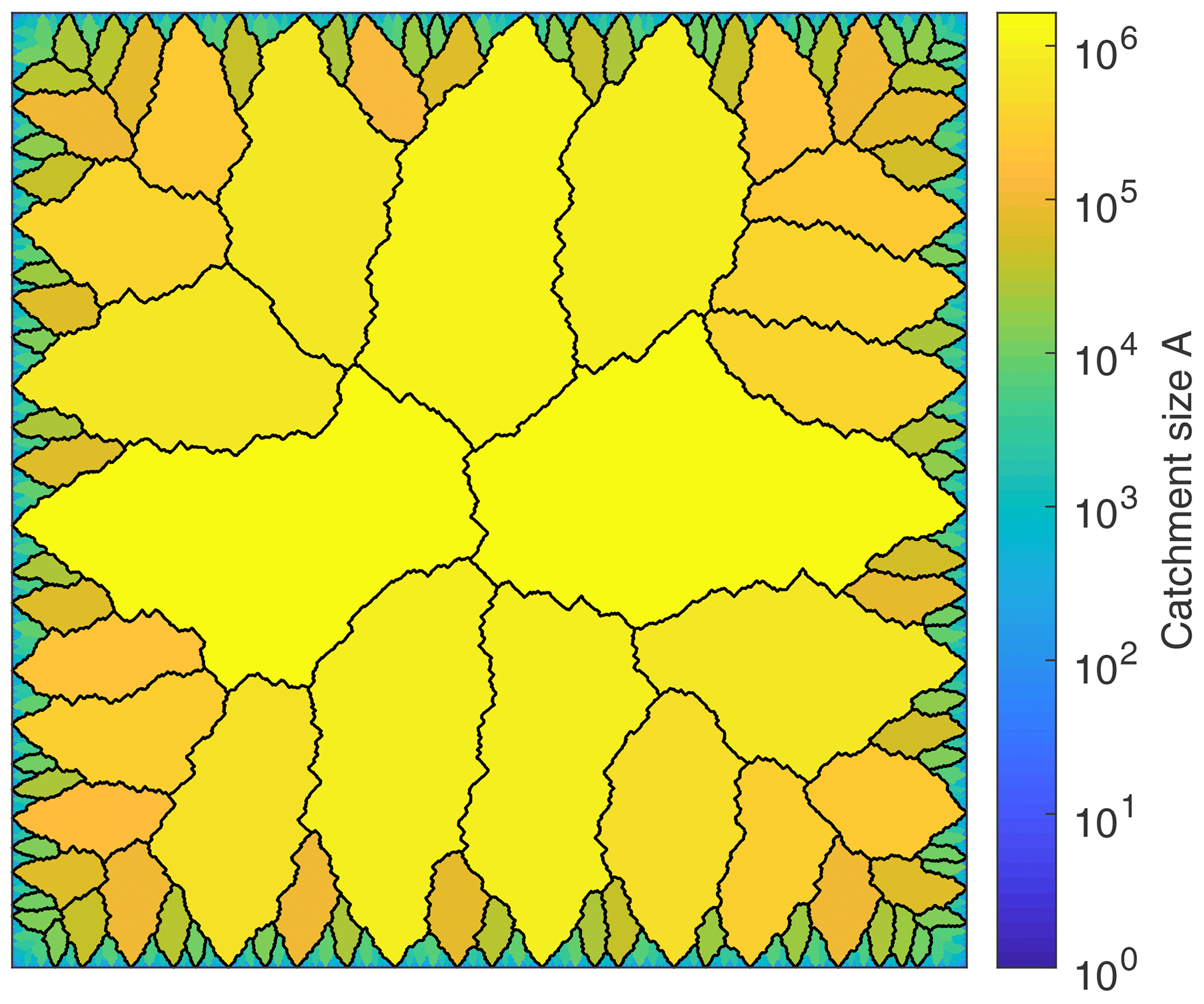
Figure 1 Catchments of numerically obtained dendritic flow patterns for n=2 on a lattice of 4096 sites × 4096 sites. The color corresponds to the size A of each individual catchment, measured in grid pixels. The watersheds between large catchments (A≥10 000 pixels) are highlighted in black.

Several scenarios will be considered for the same geometry in the following. Beside the reference scenario with n=2, the influence of n will be investigated. These investigations also include uniform transmissivity and storativity. The suitability of the description as a dendritic network will be tested against full Darcy flow.

In order to enable a comparison of the recession curves of individual springs, the same catchments are used in all simulations. This means that the boundaries between the catchments shown in Fig. 1 are enforced by cutting the respective connections, i.e., by inhibiting flow across the watersheds.

3 Results and discussion

3.1 Dendritic flow patterns vs. full Darcy flow

As a first step, we investigate under which conditions the reduction from full Darcy flow (taking all four neighbors into account) to a dendritic flow pattern (a single flow target for each node) provides a suitable approximation. We start from the optimized distribution of S and T for n=2, i.e., from a strongly preferential flow pattern. Figure 2 compares the long-term recession coefficients α (α₁ in Eq. 27) obtained from the dendritic flow pattern to those of full Darcy flow. The recession coefficients of both approaches agree well, which means that the long-term recession behavior is captured well by the dendritic flow pattern. Some deviations occur at rather small catchment sizes from about 10 to 200. Here, allowing only one single flow direction leads to a slight underestimation of α, which means that the recession is slightly too slow. This underestimation is highest at catchment sizes A≈16 and reaches about 10 % there.

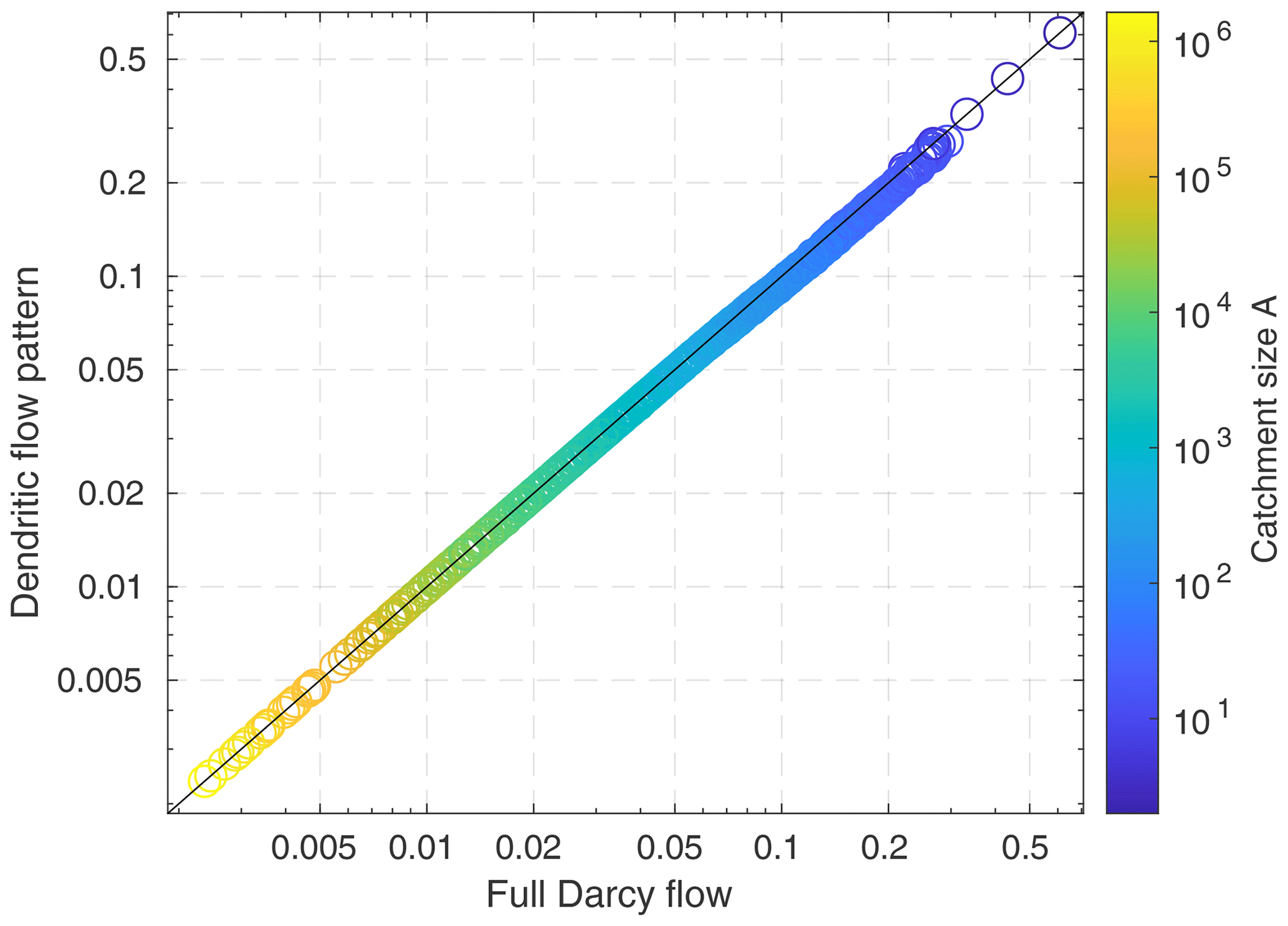
Figure 2 Recession coefficient α of each individual catchment with n=2 for dendritic flow patterns against full Darcy flow. The colors match Fig. 1 and indicate the size of the respective catchment.

In order to investigate the effect of the restricted flow directions in more detail, we analyzed the flow pattern of the full Darcy scenario. For this purpose, we define the major flux component of each node as the flux towards the given flow target (according to the dendritic pattern) and the minor flux component as the sum of the fluxes towards all other neighbors with lower head values.

Figure 3 shows the relative contribution of the minor fluxes as a function of the size of the respective upstream catchment. The upstream catchment size refers to the individual pixels here and not to the embedding catchment. Thus, the data point for a A=1 describes the average over all pixels without donors, regardless of whether they are draining directly to the boundary (i.e., are indeed single-pixel catchments) or are part of a larger catchment. As points at drainage divides are already restricted concerning their flow direction in the full Darcy scenario, these points are analyzed separately from inner points.

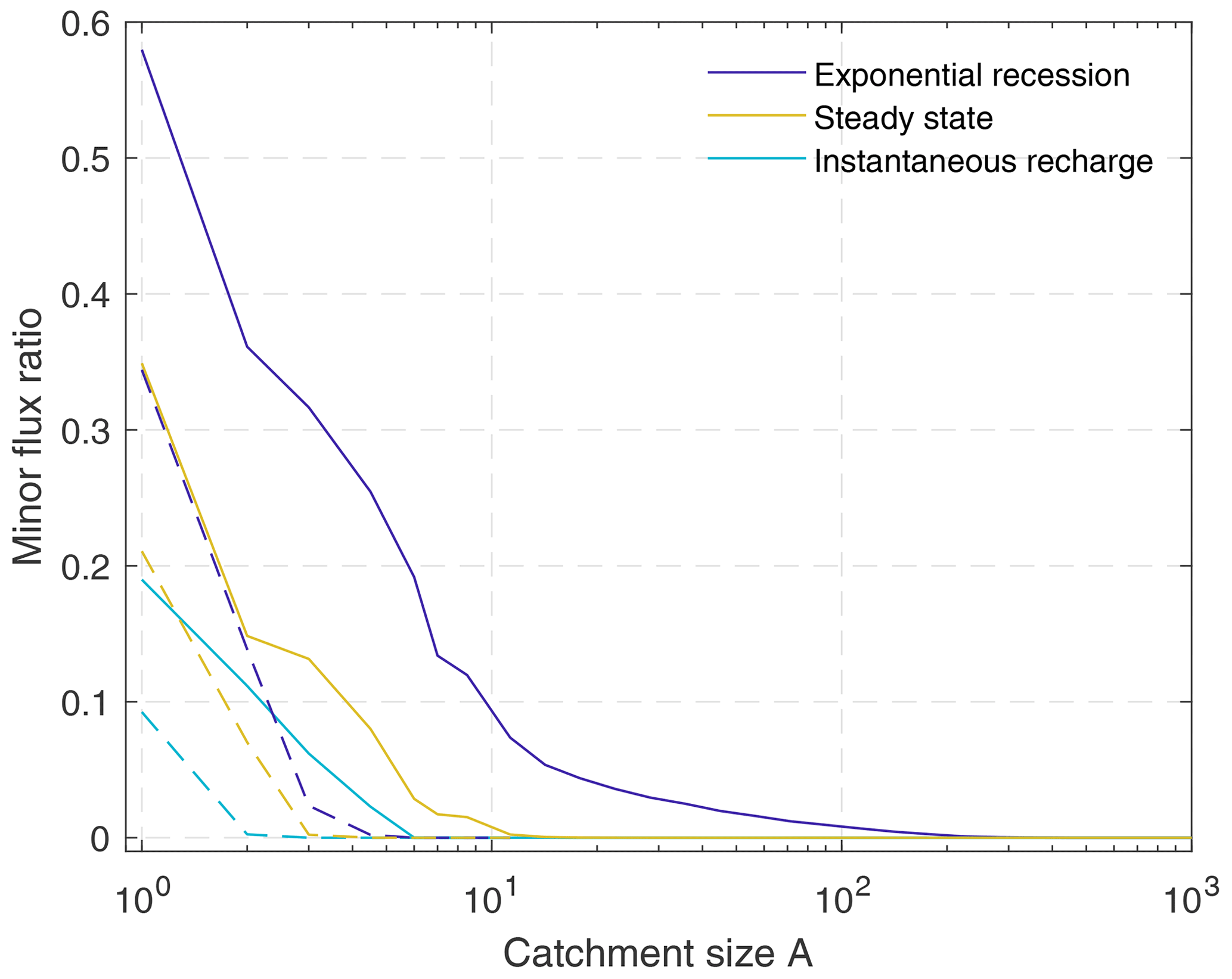
Figure 3 Relative contribution of the minor fluxes for each grid pixel as a function of the catchment size A. The curves were obtained by logarithmic binning with 10 bins per decade. All three considered scenarios – a steady-state initial condition, a unit recharge pulse, and the exponentially decaying term (only the slowest component; first term in Eq. 27) – are analyzed separately for grid pixels that lie within a catchment (flow towards all four neighbors; solid lines) and pixels at drainage divides (restricted flow directions; dashed lines).

The contribution of the minor fluxes decreases with increasing catchment size, i.e., downstream along the preferential flow paths. It becomes negligible for all considered scenarios at catchment sizes A⪆200. The contribution of the minor flux is particularly small immediately after a short, uniform recharge pulse. If all sites receive the same amount of water, the resulting change in hydraulic head is inversely proportional to the storativity. Because high transmissivity goes along with high storativity, the hydraulic gradient between sites with low transmissivity and sites with high transmissivity increases. As a consequence, the fluxes are concentrated towards the preferential flow paths, which reduces the minor fluxes.

The strongest contribution of the minor fluxes is found for the long-term recession, characterized by an exponential recession curve. The minor fluxes contribute even almost 60 % for A=1 here (only inner points, about 35 % for drainage divides). It may be surprising that the minor fluxes do not affect the recession coefficient strongly, as shown in Fig. 2. In an extreme scenario where all four neighbors are at the same head values, the fluxes would be 4 times higher in the full Darcy model than in the single-flow-target realization, which would result in a 4 times faster recession than predicted by Eq. (54). Although the majority of the nodes have small upstream catchment sizes (e.g., A=1 for 43 % of all nodes and A≤10 for 81 % of all nodes), their behavior is obviously not crucial for the properties of the entire catchment.

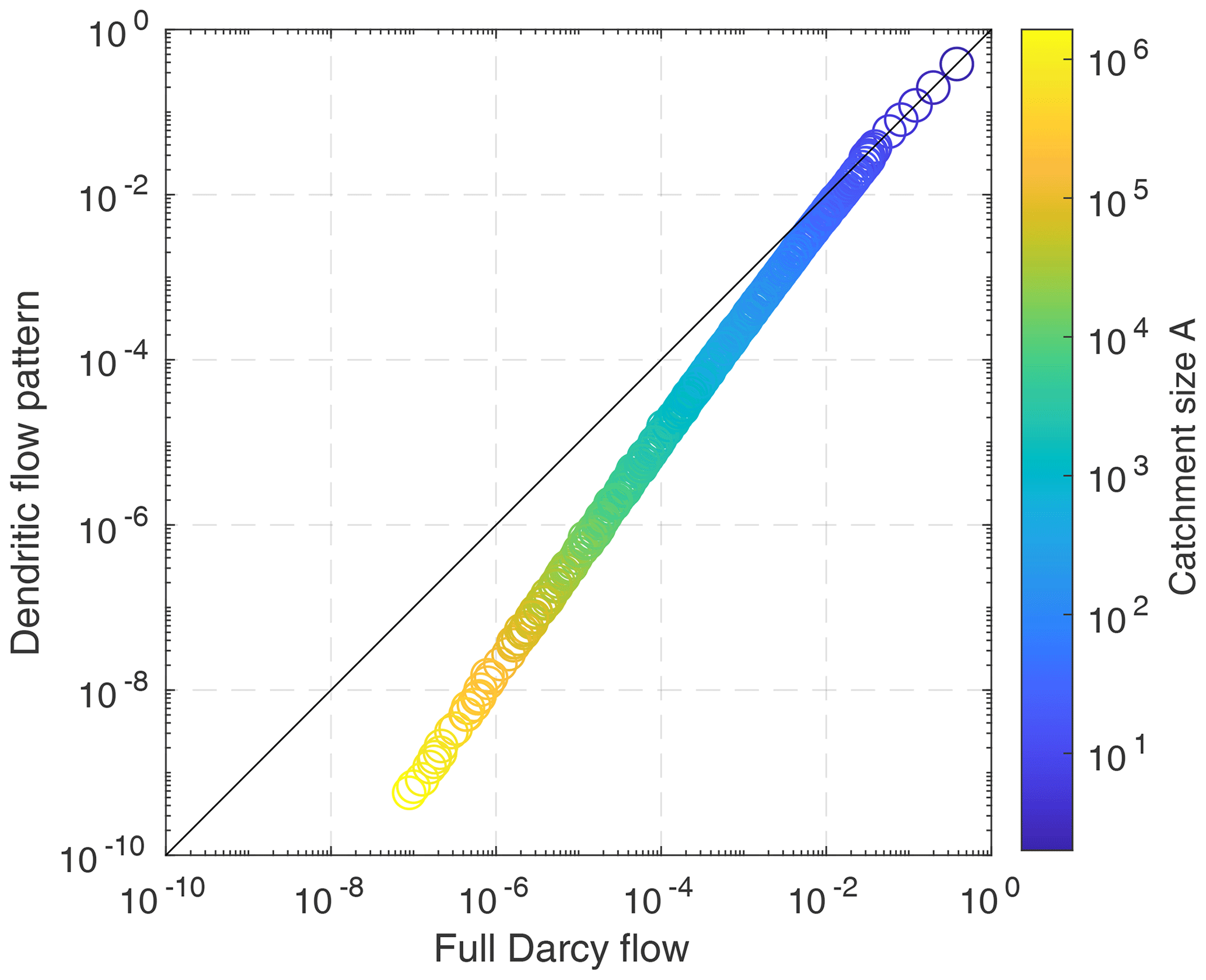
These results suggest that preferential flow patterns can be represented well on a discrete grid by a dendritic structure where each node drains only towards one of its neighbors. In turn, the approximation using a dendritic flow pattern does not work well for a spatially uniform distribution of T and S, as shown in Fig. 4. Here, α is underestimated by more than 1 order of magnitude for large catchments, which means that the recession is more than a factor of 10 too slow. The coefficients agree well only for small catchments, where the minor fluxes are small or even absent due to the restricted flow directions at drainage divides.

Figure 4 Recession coefficient α of each individual catchment with a spatially uniform distribution of T and S for dendritic flow patterns against full Darcy flow. The colors match Fig. 1 and indicate the size of the respective catchment.

3.2 Scaling properties of the recession coefficient

The fact that the recession coefficient α decreases with increasing catchment size is already visible in Figs. 2 and 4. The expected scaling behavior is $\mathit{\alpha }\propto A^{-\mathrm{1}}$. This result is formally obtained from the characteristic timescale t₀ (Eq. 46 with A∝l²), but it can also be derived directly from the occurrence of a first-order time derivative on the left-hand side of Eq. (7) and second-order spatial derivatives on the right-hand side of Eq. (7). If we rescale the entire catchment including the pattern of S and T by a factor β, the right-hand side of Eq. (7) changes by a factor of β⁻² for r=0. Then, the timescale must change by the same factor. As the catchment size A increases quadratically with β, the timescale is proportional to the catchment size and, thus, $\mathit{\alpha }\propto A^{-\mathrm{1}}$.

As shown in Fig. 5, this simple scaling behavior does not hold for the patterns of S and T considered here. While the scaling behavior follows a power law

$$\begin{array}{}\text{(55)}& \mathit{\alpha }\propto A^{-\mathit{\gamma }}\end{array}$$

reasonably well for all considered values of n, it seems that an exponent γ=1 is only achieved for n=1. For all values n>1, we find γ<1, where γ decreases with increasing n. This means that the recession of large catchments is still slower than the recession of small catchments, but the effect is considerably weaker than for a simple Darcy-type aquifer (γ=1).

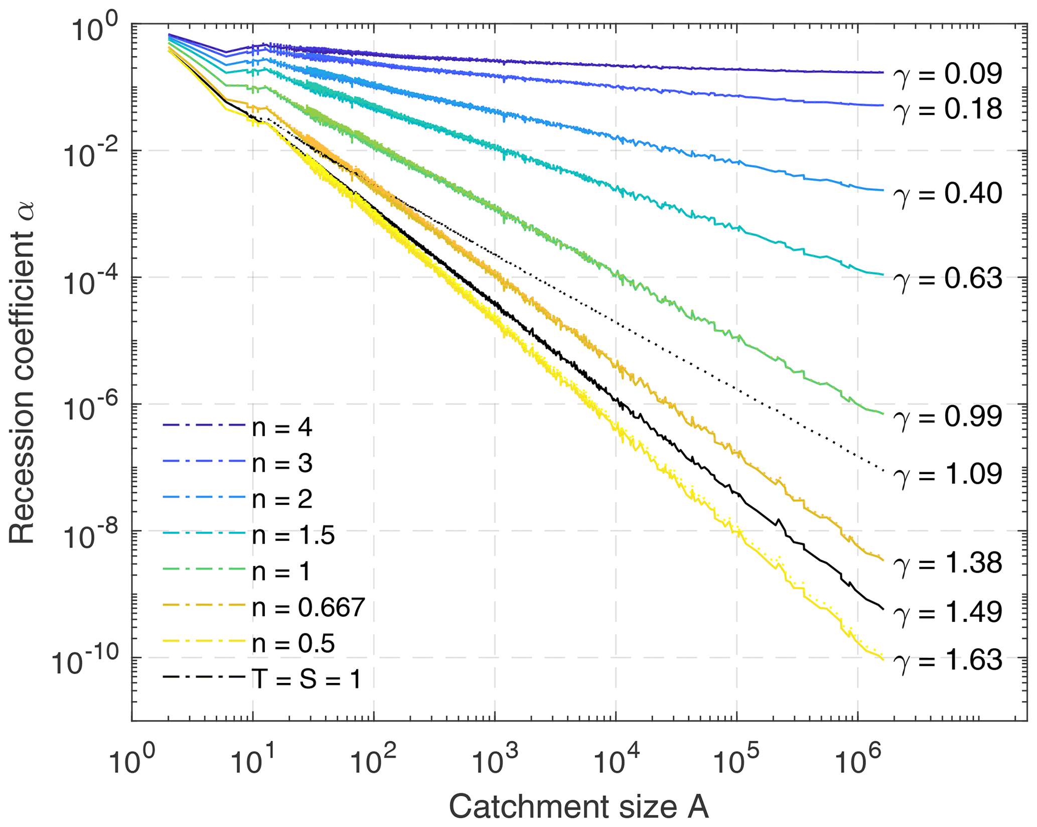
Figure 5 Scaling behavior of recession coefficient α relating to catchment size A (Eq. 55) for different values of n and for a uniform distribution of T and S. Full Darcy flow is plotted as solid lines, and flow in dendritic patterns is plotted as dotted lines. Except for the scenario with $S=T=\mathrm{1}$, the curves of full Darcy flow and the dendritic pattern are hardly distinguishable.

Qualitatively, this weaker increase is the expected behavior for a preferential flow pattern. Preferential flow paths are able to transport water rapidly over large distances, so that an increasing spatial extension does not slow down the recession as strongly as in a homogeneous aquifer.

The opposite behavior is observed for n<1. Here, large catchments become extremely slow. Revisiting Eqs. (51) and (52), it is recognized that T still increases with catchment size, but it is weaker than S for n<1. Therefore, flow is still facilitated along the preferential flow paths, but the respective cells become slow due to their high storativity. This becomes visible if we apply Eq. (54) formally to such cells, which yields $\mathit{\alpha }\propto A^{\frac{\mathrm{2}(n-\mathrm{1})}{n+\mathrm{1}}}$, so that α decreases with increasing A. However, n<1 would be unrealistic for porous media, where n≥2 should instead be expected. Beyond this, Hergarten et al. (2014) demonstrated that dendritic flow patterns are energetically favorable only for n>1. Thus, preferential flow patterns with n<1 can be constructed, but they do not make much sense. Nevertheless, the curves are almost indistinguishable not only for n≥1 but also for n<1. The results reveal that the numerical approximation using a dendritic flow pattern also works well for n<1.

As already recognized in Sect. 3.1, the approximation using a dendritic flow pattern does not work for constant transmissivity and storativity. Figure 5 reveals that the unusual scaling behavior with γ>1 also occurs for the description using full Darcy flow. This result is related to the subdivision of the domain into fixed catchments drained by distinct springs. In order to test this hypothesis, we computed the recession coefficients for radial flow towards a spring in polar coordinates. Keeping the radius of the spring constant and varying the total size of the catchment (the outer radius), we obtained roughly the same scaling behavior, γ≈1.1, found for the catchments considered in Fig. 5. This scaling behavior indicates that the region around the spring is some kind of bottleneck that becomes increasingly relevant for large catchments. This result aligns well with the result of Hergarten et al. (2014), who found that minimum energy dissipation for radial flow requires an increase in permeability towards the spring.

The nontrivial dependence of α on the catchment size not only affects spring hydrographs but also the response time of aquifers to changes in climate or hydraulic conditions at the boundaries. As a recent example, Cuthbert et al. (2019) provided worldwide estimates of these groundwater response times. These estimates are based on the 1-D version of Eq. (7) for homogeneous aquifers, with the size of the aquifer assumed to be twice the distance L of perennial rivers. The scaling arguments given above (and formally in Sect. 2.6) then yield $\mathit{\alpha }\propto L^{-\mathrm{2}}$ and, thus, a response time proportional to L². Because L increases with decreasing precipitation, this model predicts a strong negative correlation between precipitation and groundwater response time with typical response times of several thousand years in arid and semiarid regions. If the respective aquifers are not homogeneous but rather have a preferential flow structure as considered here, the dependence of the groundwater response time on L and, thus, on climate will be considerably weaker than predicted by Cuthbert et al. (2019).

3.3 Short-term recession

The differences between the model considered here and simple Darcy-type models are not limited to the scaling properties of the long-term recession coefficient. As exemplified in Fig. 6 for the biggest catchment, the unit hydrograph shows a clear rising limb at short timescales. In contrast, the 1-D Darcy-type aquifer shows a power-law decrease in discharge at short timescales, so that Q→∞ for t→0.

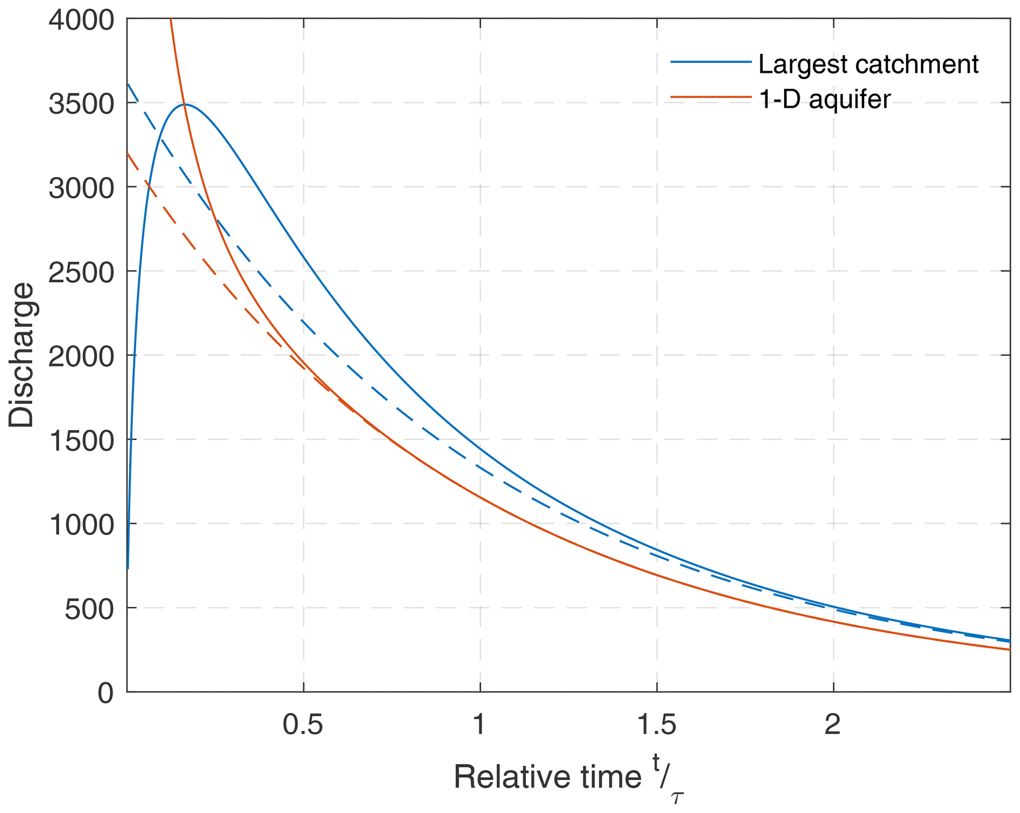
Figure 6 Unit hydrographs of the biggest catchment for n=2 and of a homogeneous 1-D aquifer. The dashed lines correspond to the long-term exponential recession. The data are scaled in such a way that the e-folding time τ and the total amount of water supplied by the recharge event are the same in both scenarios.

For a better comparison, size and parameter values of the 1-D aquifer were adjusted in such a way that the long-term recession coefficient α and the total amount of water supplied by the recharge event are the same as for the considered catchment (see Appendix B). For such a simple aquifer, a lag between a short precipitation event and the peak discharge would typically be attributed to the infiltration process. We would then assume that the time lag is related to the transit time of the water from the surface to the aquifer. In a model consisting of individual porous blocks connected by highly conductive fractures (e.g., Kovács et al., 2005; Hergarten and Birk, 2007), the time lag may also be owing to the finite conductivity of the fracture system. In contrast, the finite rise time is an inherent property of the structure of the aquifer in the model considered here. It cannot be attributed uniquely to any individual component of the system.

Figure 7 provides an analysis of the rise time t_rise for the considered catchments and different values of the exponent n. For n=2, the data suggest a linear relationship between t_rise and the long-term e-folding time $\mathit{\tau }=\frac{\mathrm{1}}{\mathit{\alpha }}$. The ratio of t_rise and τ varies from about 9 % to 19 % for the individual catchments. The rise times become slightly shorter in relation to the e-folding time for lower n. For n=1.5, we found ratios in a range from about 4 % to 22 %. The data obtained for n>2 are nonunique, in particular for small catchments (small τ). Overall, there seems to be a weak increase in the ratio of t_rise and τ with increasing n. This trend aligns well with the absence of a finite rise time in the simple 1-D and 2-D aquifers without a preferential flow pattern. However, the trend is much weaker than the variation among individual catchments; therefore, it is not investigated further. In each case, however, t_rise is not very small compared with τ. One-seventh of the e-folding recession time seems to be a reasonable order of magnitude. Taking into account that long-term e-folding times of karst aquifers are typically in an order of magnitude of several weeks, the rise time is of an order of magnitude of several days.

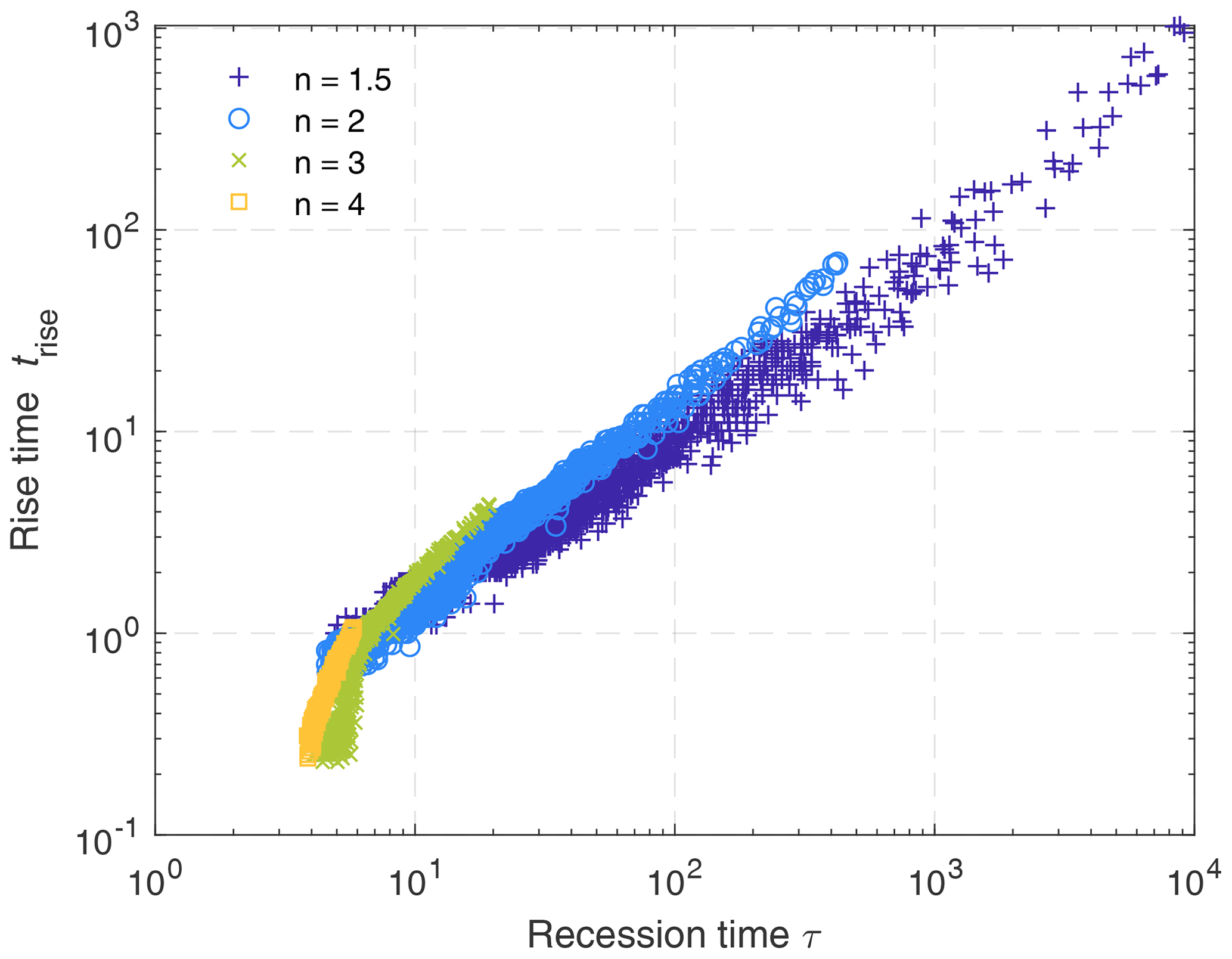
Figure 7 Relation between rise time t_rise and e-folding time τ of the long-term recession for the considered catchments and different values of n.

The occurrence of a rising limb in the unit hydrograph requires that some of the coefficients λ_kQ_k in Eq. (27) are negative. This can be seen formally by computing the derivative of Eq. (27). The derivative is similar to Eq. (27) itself, except that the coefficients are −α_kλ_kQ_k. As the sum cannot become zero if all coefficients have the same sign, at least one of the original coefficients λ_kQ_k must be negative. Figure 8 shows the coefficients for the largest catchment. While the coefficients of the slowest components (small α_k) are positive, there is no obvious preference for either sign in the faster components.

The spectrum of the considered catchment differs fundamentally from that of the 1-D aquifer. While the spectrum of the 1-D aquifer consists of distinct components with recession coefficients ${\mathit{\alpha }}_k\propto (\mathrm{2}k-\mathrm{1}{)}^{\mathrm{2}}$ (see Appendix B), the spectrum of the catchment becomes more or less continuous at large k. However, the smallest recession coefficients are still distinct. For the catchment analyzed in Fig. 8, the ratio is $\frac{{\mathit{\alpha }}_{\mathrm{2}}}{{\mathit{\alpha }}_{\mathrm{1}}}\approx \mathrm{2}$. While the lowest ratios among all simulated catchments are about 1.5, the ratio is typically in a range from about 2.5 to 4 for smaller catchments. Thus, the ratio $\frac{{\mathit{\alpha }}_{\mathrm{2}}}{{\mathit{\alpha }}_{\mathrm{1}}}$ differs from catchment to catchment but is always clearly above unity. This also holds for n≠2. This property ensures that the recession curve approaches a single exponential function at a reasonable time and that the coefficient λ₁Q₁ captures the long-term recession well. However, the ratio is much lower than the ratio $\frac{{\mathit{\alpha }}_{\mathrm{2}}}{{\mathit{\alpha }}_{\mathrm{1}}}=\mathrm{9}$ of the 1-D aquifer. Although the deviation from an exponential recession also depends on the coefficients λ_kQ_k, the difference is already visible in Fig. 6. While the unit hydrograph of the 1-D aquifer is almost indistinguishable from the exponential decay at t=0.5τ, the difference is more than 15 % at this time for the largest catchment. Therefore, the model with the preferential flow pattern approaches the long-term exponential recession much more slowly than the simple 1-D aquifer.

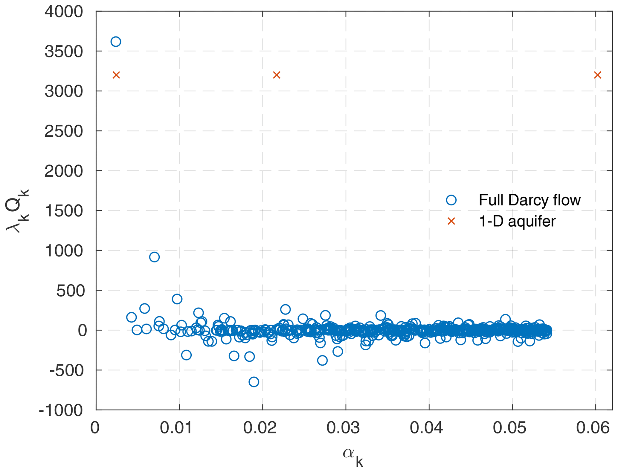
Figure 8 Coefficients λ_kQ_k and recession coefficients α_k in Eq. (27) for the largest catchment (n=2). Only the slowest 500 components (k≤500) were computed. The data of the 1-D aquifer were rescaled in such a way that the lowest recession coefficient α₁ and the total recharge are the same as for the simulated catchment.

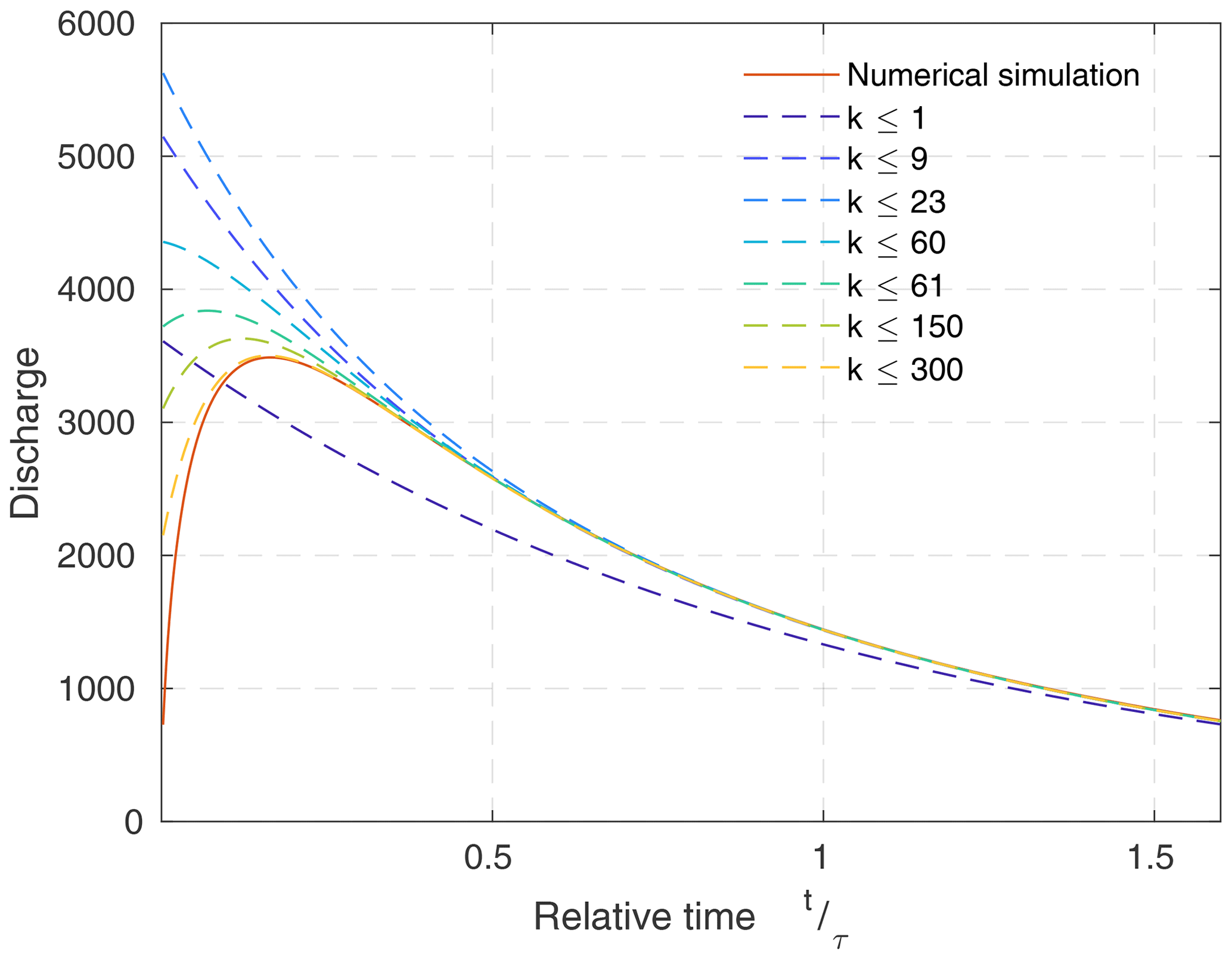
Figure 9 Recession curves of the largest catchment obtained from the numerical simulation and different numbers of exponential functions (Eq. 27).

Figure 9 illustrates the approximation of the unit hydrograph by a finite number of exponential components. In this example, all coefficients for k≤9 are positive. In the range $\mathrm{9}<k\le \mathrm{23}$, there are also negative coefficients. However, the positive coefficients still dominate here, so that the highest peak discharge is achieved when including the components with k≤23. The negative components become increasingly relevant for larger k. This results in a decreasing peak discharge, however, that is still at t=0 for k≤60. The component with k=61 is the first that shifts the peak discharge to a time t>0 and, thus, produces a rising limb in the unit hydrograph. However, approximating the behavior around the peak discharge reasonably well requires several hundred components.

The occurrence of negative coefficients in Eq. (27) is not a fundamental problem, but it impedes a simple interpretation of the decomposition into exponentially decreasing terms. If all components were positive, we could imagine the aquifer as a set of linear reservoirs drained in parallel. However, negative components would correspond to reservoirs with a negative amount of water. Formally, the slow component (first exponential function) could even contain more water than available in total, and the fast components (all higher exponentials) could be negative in total. In Fig. 6, this would mean that the area of the unit hydrograph below the exponential component at short timescales was larger than the area above the exponential component. In this case, the widely used characterization of karst aquifers according to the contribution of the slow (exponential) component to the total discharge (Mangin, 1975; Jeannin and Sauter, 1998) would be taken ad absurdum.

Figure 10 shows the contribution of the slow component (first exponential) to the total amount of water for all catchments considered here (n=2). Depending on the catchment size, this contribution is between 77 % and 104 %. Thus, there are indeed catchments where the effect of the rising limb is so strong that the slow component is formally larger than the total recharge and the fast components are negative in sum. However, this effect is found only for some rather small catchments. For the largest catchments, the contribution of the slow component is about 90 %.

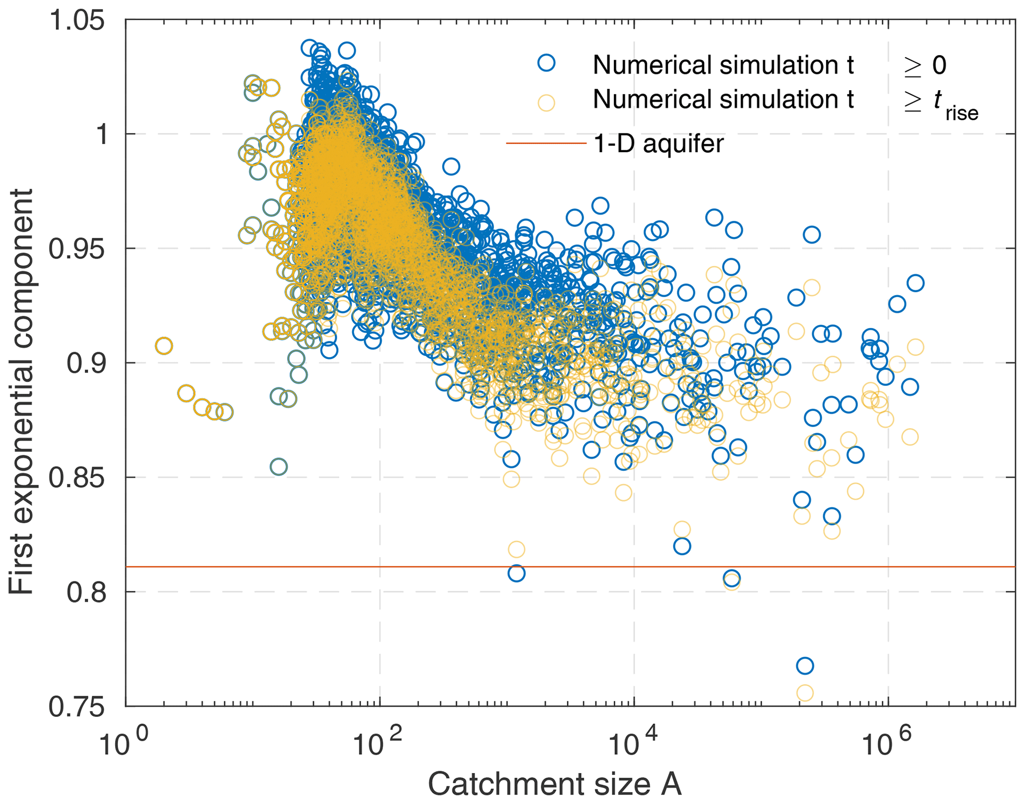
Figure 10 Contribution of the slowest exponential component to the total discharge for the considered catchments. The red line shows the respective contribution of $\frac{\mathrm{8}}{{\mathit{\pi }}^{\mathrm{2}}}\approx \mathrm{81}$ % for the 1-D aquifer.

The obtained contributions of the slow component are high compared with other models. For the 1-D aquifer used here as a reference, this contribution is $\frac{\mathrm{8}}{{\mathit{\pi }}^{\mathrm{2}}}\approx \mathrm{81}$ %. For an aquifer consisting of square porous blocks connected by conduits with infinite conductance, it is $\frac{\mathrm{64}}{{\mathit{\pi }}^{\mathrm{4}}}\approx \mathrm{66}$ % (e.g., Birk and Hergarten, 2010). The contribution of the slow component was not explicitly investigated by Hergarten and Birk (2007) in their fractal model with power-law-distributed block sizes. However, as the slowest flow component arises from the largest blocks, the total contribution of the slow component must even be considerably smaller than the 66 % obtained for an aquifer with a uniform block size. In the widely used classification scheme of karst aquifers proposed by Mangin (1975), even aquifers with a contribution of the slow component of less than 50 % are considered poorly karstified (see also Jeannin and Sauter, 1998). Therefore, our continuous model of preferential flow patterns predicts an even higher contribution of the slow component to the unit hydrograph than other models and is very different from what is typically assumed for karst systems.

At first sight, the observed high contribution of the slow component could be an effect of the finite rise time. As recognized in Figs. 6 and 9, the unit hydrograph is below the slow component for t⪅0.5t_rise. When investigating recession curves in reality, the analysis typically starts from the peak in discharge (t=t_rise). The orange markers in Fig. 10 show the respective contributions of the slow component. Starting the analysis from t=t_rise instead of t=0 indeed yields lower contributions of the slow components. However, the effect is only of the order of magnitude of a few percent. Thus, the result that continuous preferential flow patterns predict a high contribution of the slowest flow component is not an artifact of the analysis.

3.4 The effect of nonuniform recharge

While the unit hydrograph describes uniform recharge, the spatial distribution of the recharge may have a strong influence on recession curves of large catchments. Therefore, a question arises regarding whether the strong deviations from the exponential behavior found for karst springs could be related to the occurrence of local rainstorms that affect only a small part of the catchment.

As a simple example, we separated the domain into a proximal part and a distal part. Both parts are equally sized, and a distinction is made based on the distance from the boundary of the domain. Because the overall domain is the same, the recession coefficients α_k of all flow components are the same as for the entire domain. Only the coefficients a_k in Eq. (27) differ. This difference, however, has a strong effect on the rise time and on the contribution of the slow flow component.

Figure 11 compares the results obtained numerically for the largest catchment to those obtained by spectral decomposition for a 1-D aquifer (for details, see Appendix B). While the hydrograph starts with a peak at t=0 after a spatially uniform recharge event, applying recharge only to the distal part of the domain introduces a finite rise time. This rise time is, however, shorter (in relation to the e-folding recession time) than for the aquifer with the preferential flow pattern. The rise time of the preferential flow pattern also changes considerably if recharge is only applied to a part of the domain. The strong influence may be surprising at first because we could expect the signal to propagate rapidly through the preferential flow structure from the distal part of the domain to the spring. However, preferential flow paths not only have a high transmissivity here but also a high storativity. Thus, the propagation of signals is not as fast as we might expect.

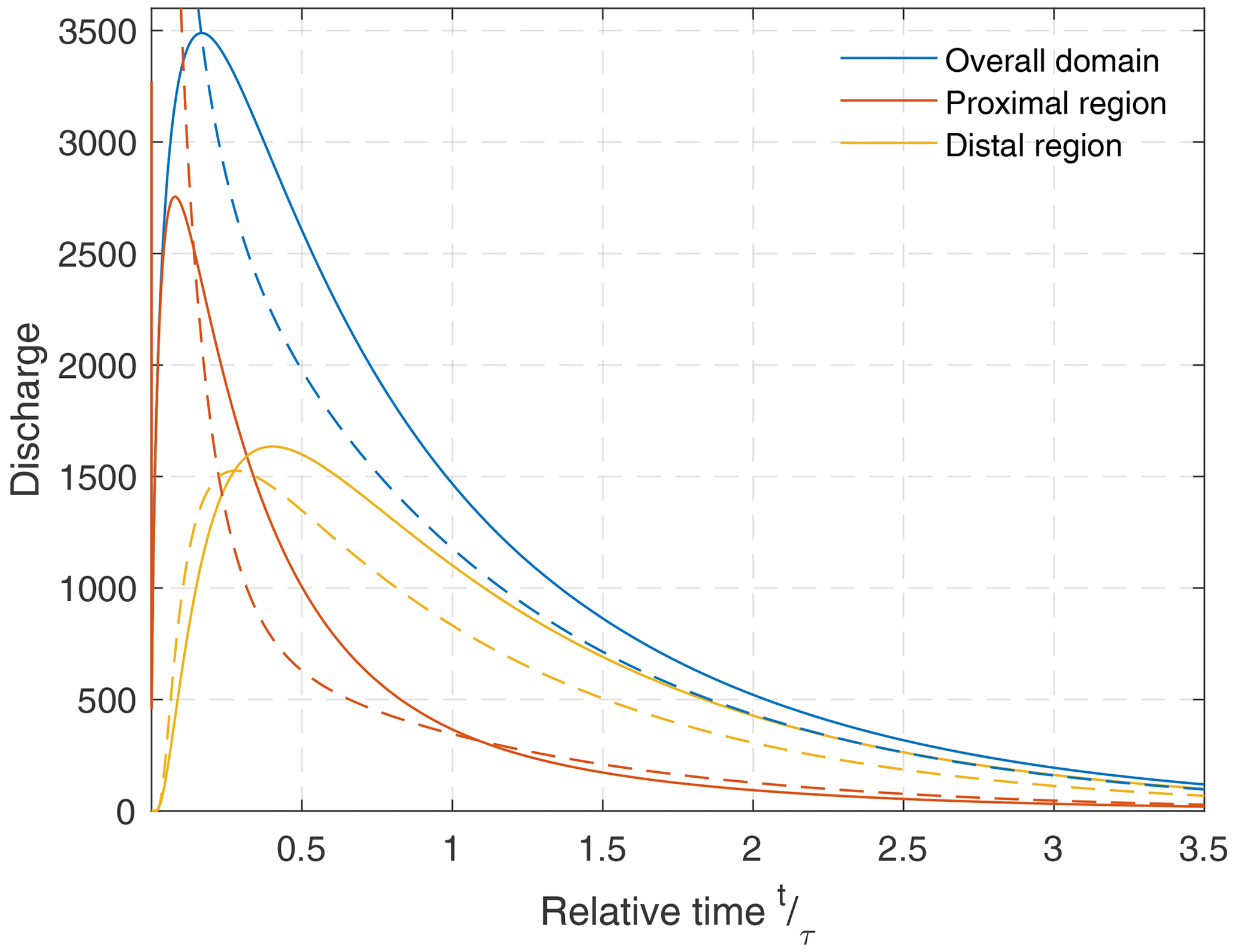
Figure 11 Instantaneous unit hydrographs for recharge applied to a part of the domain. Solid lines refer to the largest catchment of the simulation and dashed lines refer to a homogeneous aquifer. The data are scaled in such a way that the e-folding time τ and the total amount of supplied water are the same in both scenarios. Proximal and distal regions cover half of the catchment each.

The contribution of the slowest component also changes if recharge is only applied to a part of the domain. Similarly to the rise time, it increases if only the distal part of the domain is filled because the instantaneous recharge signal has already been smoothed when it arrives at the spring. The contribution of the first exponential component is formally higher than 100 % for the distal part. For the largest simulated catchment, it is 137 %, whereas it is 115 % for the 1-D aquifer. In turn, the contribution of the first exponential component is lower for the proximal parts: 50 % for the largest catchment in the simulation and 47 % for the 1-D aquifer. Therefore, the contribution of the first exponential component is always higher for the preferential flow pattern than for the 1-D aquifer, and the effect of only applying recharge to a part of the domain is similar.

On average, however, the effect vanishes. For the largest catchment, the 50 % for the proximal region and the 137 % for the distal region yield a mean value of 94 %, in agreement with Fig. 10 (the rightmost blue circle). This is a general property of the linear model, which allows for the superposition of recharge events not only temporally but also spatially. It could even be generalized to arbitrary parts of the domain down to recharge events that are limited to a single node.

While there should theoretically be no effect on average, recharge events in the proximal region will be more prominent in the hydrograph than those in the distal region. Therefore, the analysis of real-world hydrographs might be biased towards the more prominent, proximal recharge events, which would yield a decreasing contribution of the slowest component for large catchments. However, explaining the often small contribution of the exponential component this way seems quite a stretch.

4 Conclusions and perspectives

This study is a first attempt to describe the dynamics of aquifers with continuous preferential flow patterns. In contrast to approaches based on two or three distinct flow components widely used in the context of karst aquifers, the concept used here assumes a continuous spatial variation in hydraulic properties over several orders of magnitude.

A 2-D aquifer with a spatially variable but time-independent transmissivity was considered. This scenario corresponds to the application of small disturbances to a steady state of an aquifer with an almost horizontal water table. Synthetic spatial patterns of transmissivity and storativity were obtained from principles of minimum energy dissipation based on the theory proposed by Hergarten et al. (2014).

As a major technical result, it was found that such aquifers can be approximated well by dendritic flow patterns, in which the entire discharge of each cell is delivered to the neighbor with the steepest gradient in hydraulic head. This approximation has been widely used for channelized flow patterns at the surface. The dendritic structure enables an efficient, fully implicit numerical scheme with a numerical effort that increases only linearly with the number of cells, also known as O(n) complexity. This property allows for simulations on grids consisting of several million nodes and, thus, for a reasonable spatial resolution of the preferential flow pattern.

As a second, rather theoretical result, it was shown that spectral theory is not restricted to homogeneous aquifers and can also be applied to aquifers with any spatial distribution of transmissivity and storativity. Although the eigenvalues and the respective eigenvectors have to be computed numerically, this approach allows for a fast computation of the long-term recession coefficient without forward modeling over a long time span. In addition, the contribution of the slowest flow component to the instantaneous unit hydrograph (and also to any other initial state) can be computed easily. However, the efficient numerical scheme and spectral theory rely on the assumption of time-independent transmissivity and cannot be extended easily towards sloping aquifers.

The long-term recession coefficient α depends on the catchment size. The dependency is, however, weaker than for homogeneous aquifers and follows a power law $\mathit{\alpha }\propto A^{-\mathit{\gamma }}$ (Eq. 55). The exponent γ depends on the assumed relation between transmissivity T and storativity S. It approaches 1 for T∝S, which is also the limit where dendritic flow patterns are energetically favorable. In this case, the scaling is the same as for homogeneous aquifers (γ=1). For relations T∝Sⁿ, γ decreases with increasing n. As a typical value, γ=0.4 was found for n=2. Therefore, the decrease in the recession coefficient with catchment size is typically less than half as strong as for homogeneous aquifers. This finding challenges previous results on very long groundwater response times of large aquifers (e.g., Cuthbert et al., 2019).

Because flow patterns obtained from minimum energy dissipation are typically scale-invariant, a power-law decrease in the discharge after a short recharge pulse might be expected at first. However, the respective instantaneous unit hydrograph shows a completely different behavior. The discharge immediately after the recharge event is quite small, and it takes a considerable time until it reaches its peak. The order of magnitude of this rise time is one-seventh of the characteristic time of the aquifer ($\mathit{\tau }={\mathit{\alpha }}^{-\mathrm{1}}$). It seems not to depend strongly on the catchment size nor on the relation between transmissivity and storativity.

The contribution of the slowest component to the unit hydrograph is of an order of magnitude of 90 % for large catchments and even larger for small catchments. This contribution increases further if recharge is only applied to a part of the domain at a distance from the spring and can even exceed 100 % in these cases. Formally, this result arises from the occurrence of negative coefficients in the decomposition of the unit hydrograph into exponentially decaying components. The occurrence of negative coefficients also inhibits the simple interpretation as a set of linear reservoirs draining in parallel. Measuring the contribution of the slowest component from the peak of the unit hydrograph instead of the time at which the instantaneous recharge occurs reduces the contribution of the slowest component only slightly. This contribution is higher than for homogeneous aquifers and much higher than typically assumed for karst aquifers (less than 50 %).

Thus, we have to conclude that preferential flow patterns arising from a strongly organized pattern of transmissivity and storativity differ fundamentally from karst aquifers in their properties. For future work, it would be interesting to find out whether the difference mainly concerns the contribution of the slowest flow component or also the scaling of the recession coefficient with catchment size.

With respect to further development, an extension of the numerical scheme towards unconfined sloping aquifers (e.g., Rupp and Selker, 2006; Pauritsch et al., 2015) would be particularly useful. Although there is ongoing development in this field (e.g., Alemie et al., 2019; Pathania et al., 2019), including preferential flow patterns at a reasonable spatial resolution is still a challenge. Extending the implicit scheme for dendritic flow patterns towards unconfined sloping aquifers would still be challenging, but it might considerably contribute to understanding the response of hillslopes to precipitation events and phenomena such as subsurface storm flow (e.g., Chifflard et al., 2019).

Appendix A: The fully implicit scheme for a dendritic network

In this section, Eqs. (42) and (43), which are the basis of the implicit scheme discussed in Sect. 2.5, are proven. Inserting Eqs. (14) and (41) into Eq. (40) yields

$$\begin{array}{}\text{(A1)}& \begin{array}{rl}{S}_i{\displaystyle \frac{h_i(t+\mathit{\delta }t)-h_i\left(t\right)}{\mathit{\delta }t}}& =-T_i\left(h_i(t+\mathit{\delta }t)-h_b(t+\mathit{\delta }t)\right)\\ & +\sum _{j\in D\left(i\right)}{q}_j^{\mathrm{0}}+\sum _{j\in D\left(i\right)}{q}_j^{\prime }\\ & \left(h_i(t+\mathit{\delta }t)-h_i\left(t\right)\right)+r_i,\end{array}\end{array}$$

and thus

$$\begin{array}{}\text{(A2)}& h_i(t+\mathit{\delta }t)-h_i\left(t\right)={\displaystyle \frac{T_i\left(h_b(t+\mathit{\delta }t)-h_i\left(t\right)\right)+\sum _j{q}_j^{\mathrm{0}}+r_i}{\frac{S_i}{\mathit{\delta }t}+T_i-\sum _j{q}_j^{\prime }}}.\end{array}$$

Using Eq. (14), we can then compute the flux according to

$$\begin{array}{}\text{(A3)}& \begin{array}{rl}{q}_i& (t+\mathit{\delta }t)=T_i\left(h_i(t+\mathit{\delta }t)-h_b(t+\mathit{\delta }t)\right)\\ & =T_i\left({\displaystyle \frac{T_i\left(h_b(t+\mathit{\delta }t)-h_i\left(t\right)\right)+\sum _j{q}_j^{\mathrm{0}}+r_i}{\frac{S_i}{\mathit{\delta }t}+T_i-\sum _j{q}_j^{\prime }}}\right.\\ & \left.+h_i\left(t\right)-h_b(t+\mathit{\delta }t)\right)\\ & =T_i{\displaystyle \frac{\left(\frac{S_i}{\mathit{\delta }t}-\sum _j{q}_j^{\prime }\right)\left(h_i\left(t\right)-h_b(t+\mathit{\delta }t)\right)+\sum _j{q}_j^{\mathrm{0}}+r_i}{\frac{S_i}{\mathit{\delta }t}+T_i-\sum _j{q}_j^{\prime }}}.\end{array}\end{array}$$

Then, $q_i^{\mathrm{0}}$ (Eq. 42) is obtained by setting $h_b(t+\mathit{\delta }t)=h_b\left(t\right)$ and $q_i^{\prime }$ (Eq. 43) is obtained by taking the derivative with respect to h_b(t+δt).

Appendix B: The unit hydrograph of a homogeneous 1-D aquifer

Let us consider a 1-D aquifer with a length L, where the spring is located at x=0 and the drainage divide at x=L. The boundary conditions are then $h(x,t)=\mathrm{0}$ at x=0 and $\frac{\partial }{\partial x}h(x,t)=\mathrm{0}$ at x=L, and h(x,t) is periodic with a wavelength of 4L. Thus, h(x,0) can be written as a Fourier series:

$$\begin{array}{}\text{(B1)}& h(x,\mathrm{0})=\sum _{k=\mathrm{1}}^{\mathrm{\infty }}{a}_k\sin \left({\displaystyle \frac{\mathrm{2}\mathit{\pi }kx}{\mathrm{4}L}}\right),\end{array}$$

where the respective terms with the cosine function are zero due to the boundary conditions and a_k=0 for even values of k. The coefficients a_k are given by the relation

$$\begin{array}{}\text{(B2)}& {\displaystyle }& {\displaystyle }{a}_k={\displaystyle \frac{\mathrm{2}}{\mathrm{4}L}}\underset{\mathrm{0}}{\overset{\mathrm{4}L}{\int }}h(x,\mathrm{0})\sin \left({\displaystyle \frac{\mathrm{2}\mathit{\pi }kx}{\mathrm{4}L}}\right)\mathrm{d}x\text{(B3)}& {\displaystyle }& {\displaystyle }={\displaystyle \frac{\mathrm{2}}{L}}\underset{\mathrm{0}}{\overset{L}{\int }}h(x,\mathrm{0})\sin \left({\displaystyle \frac{\mathrm{2}\mathit{\pi }kx}{\mathrm{4}L}}\right)\mathrm{d}x.\end{array}$$

If we assume that the distal region, $\mathit{\lambda }L\le x\le L$ with $\mathit{\lambda }\in [\mathrm{0},\mathrm{1}]$, is initially filled to a given head value h₀, we obtain

$$\begin{array}{}\text{(B4)}& a_k={\displaystyle \frac{\mathrm{2}{h}_{\mathrm{0}}}{L}}\underset{\mathit{\lambda }L}{\overset{L}{\int }}\sin \left({\displaystyle \frac{\mathrm{2}\mathit{\pi }kx}{\mathrm{4}L}}\right)\mathrm{d}x={\displaystyle \frac{\mathrm{4}{h}_{\mathrm{0}}}{\mathit{\pi }k}}\cos \left({\displaystyle \frac{\mathit{\pi }k\mathit{\lambda }}{\mathrm{2}}}\right)\end{array}$$

for uneven values of k. The time-dependent solution h(x,t) must satisfy the 1-D version of Eq. (7) with r=0,

$$\begin{array}{}\text{(B5)}& S{\displaystyle \frac{\partial h}{\partial t}}={\displaystyle \frac{\partial }{\partial x}}\left(T{\displaystyle \frac{\partial h}{\partial x}}\right).\end{array}$$

It is easily recognized that the solution of this equation with the initial condition defined by Eq. (B1) is

$$\begin{array}{}\text{(B6)}& h(x,t)=\sum _{k=\mathrm{1}}^{\mathrm{\infty }}{a}_k\sin \left({\displaystyle \frac{\mathrm{2}\mathit{\pi }kx}{\mathrm{4}L}}\right)e^{-{\mathit{\alpha }}_{k}t},\end{array}$$

where

$$\begin{array}{}\text{(B7)}& {\mathit{\alpha }}_k={\displaystyle \frac{T}{S}}{\left({\displaystyle \frac{\mathit{\pi }k}{\mathrm{2}L}}\right)}^{\mathrm{2}}.\end{array}$$

The flux per unit width across the boundary is then

$$\begin{array}{}\text{(B8)}& {\displaystyle }q\left(t\right)& {\displaystyle }=T{\left.{\displaystyle \frac{\partial }{\partial x}}h(x,t)\right|}_{x=\mathrm{0}}\text{(B9)}& {\displaystyle }& {\displaystyle }=T\sum _{k=\mathrm{1}}^{\mathrm{\infty }}{a}_k{\displaystyle \frac{\mathrm{2}\mathit{\pi }k}{\mathrm{4}L}}{e}^{-{\mathit{\alpha }}_{k}t}\text{(B10)}& {\displaystyle }& {\displaystyle }={\displaystyle \frac{\mathrm{2}T{h}_{\mathrm{0}}}{L}}\sum _{\stackrel{k=\mathrm{1}}{\left(\mathrm{uneven}\right)}}^{\mathrm{\infty }}\cos \left({\displaystyle \frac{\mathit{\pi }k\mathit{\lambda }}{\mathrm{2}}}\right)e^{-{\mathit{\alpha }}_{k}t}\end{array}$$

with the coefficients a_k from Eq. (B4). The respective expression for the proximal region, $\mathrm{0}\le x\le \mathit{\lambda }L$, is readily obtained by subtracting this expression from the same expression with λ=0.