Uncertainty in water transit time estimation with StorAge Selection functions and tracer data interpolation

Transit time distributions (TTDs) of streamflow are useful descriptors for understanding flow and solute transport in catchments. Catchment-scale TTDs can be modeled using tracer data (e.g. oxygen isotopes, such as δ¹⁸O) in inflow and outflows by employing StorAge Selection (SAS) functions. However, tracer data are often sparse in space and time, so they need to be interpolated to increase their spatiotemporal resolution. Moreover, SAS functions can be parameterized with different forms, but there is no general agreement on which one should be used. Both of these aspects induce uncertainty in the simulated TTDs, and the individual uncertainty sources as well as their combined effect have not been fully investigated. This study provides a comprehensive analysis of the TTD uncertainty resulting from 12 model setups obtained by combining different interpolation schemes for δ¹⁸O in precipitation and distinct SAS functions. For each model setup, we found behavioral solutions with satisfactory model performance for in-stream δ¹⁸O (KGE > 0.55, where KGE refers to the Kling–Gupta efficiency). Differences in KGE values were statistically significant, thereby showing the relevance of the chosen setup for simulating TTDs. We found a large uncertainty in the simulated TTDs, represented by a large range of variability in the 95 % confidence interval of the median transit time, varying at the most by between 259 and 1009 d across all tested setups. Uncertainty in TTDs was mainly associated with the temporal interpolation of δ¹⁸O in precipitation, the choice between time-variant and time-invariant SAS functions, flow conditions, and the use of nonspatially interpolated δ¹⁸O in precipitation. We discuss the implications of these results for the SAS framework, uncertainty characterization in TTD-based models, and the influence of the uncertainty for water quality and quantity studies.

1 Introduction

Understanding how catchments store and release water of different ages has significant implications for flow and solute transport, as water ages encapsulate information about flow paths' characteristics (McGuire and McDonnel, 2006; Botter et al., 2011), the contact time of solutes with the soil matrix (Benettin et al., 2015a; Hrachowitz et al., 2016), and vulnerability assessment (Kumar et al., 2020). This plays an important role in water resources protection and management, and it requires a tool that can effectively describe catchment-scale transport processes (Rinaldo and Marani, 1987). The age of water in outflows is commonly referred to as transit time (TT), i.e. the time that elapses between the entry of a water parcel into the catchment via precipitation and its exit via streamflow or evapotranspiration. Accordingly, the transit time distribution (TTD) describes the whole spectrum of transit times in outflows (Botter et al., 2005; Van der Velde et al., 2010). Early studies have often assumed simplified steady-state transport models, resulting in time-invariant TTDs (Niemi, 1977; Rinaldo et al., 2006). However, experimental simulations have shown that TTDs are time-variant due to the variability in meteorological forcing (Botter et al., 2010; Hrachowitz et al., 2010; Heidbüchel et al., 2020) and the activation/deactivation of flow paths in response to varying hydrologic conditions (Ambroise, 2004; Heidbüchel et al., 2013). Recent research has introduced new models for representing time-variant TTDs, for example, allowing for the estimation of TTDs without making prior assumptions about their shape (Kirchner, 2019; Kim and Troch, 2020) or with the parameterization of the StorAge Selection (SAS) functions (Rinaldo et al., 2015; Harman, 2019). SAS functions describe how catchments selectively remove water of different ages from storage for outflows, and they have led to a new framework of nonstationary transport models based on water age, which have been successfully applied in various studies (Benettin et al., 2015b; Queloz et al., 2015; Kim et al., 2016; Lutz et al., 2017; Wilusz et al., 2017; Nguyen et al., 2021).

Model-based TTDs are subjected to uncertainty, which limits their ability with respect to decision support. In general, model prediction uncertainty stems from model inputs, structure, and parameters (Beven and Freer, 2001). As TTDs are not directly observable, conservative environmental tracers (e.g. oxygen isotopes, such as δ¹⁸O) in inflow and outflows are commonly used to infer water ages (Hrachowitz et al., 2013; Birkel and Soulsby, 2015; Stockinger et al., 2015). Long-term, high-frequency tracer data with an appropriate spatial distribution are generally recommended for a sufficient understanding of TTD dynamics across a wide range of fast and heterogeneous hydrological behaviors (Kirchner et al., 2004; Danesh-Yazdi et al., 2016; von Freyberg et al., 2017). Therefore, a lack of appropriate tracer data coverage can hamper our understanding of TTD dynamics at the desired resolution (McGuire and McDonnel, 2006). Additionally, uncertainty in the driving hydroclimatic fluxes, such as precipitation, discharge, and evapotranspiration, could propagate into the uncertainty in the modeling results. Further uncertainty emerges from the model structure due to the difficulty in representing physical processes because of our incomplete knowledge of complex reality (Ajami et al., 2007). Finally, specification of model parameters is also an important source of uncertainty (Beven, 2006; Kirchner, 2006), as the best-fit parameters may suffer from equifinality (Schoups et al., 2008).

A few studies have investigated the uncertainty in the estimated TTDs with SAS models. Danesh-Yazdi et al. (2018) and Jing et al. (2019) analyzed the effect of interactions between distinct flow domains, external forcing, and recharge rate on the resulting TTDs. Several works (Benettin et al., 2017; Wilusz et al., 2017; Rodriguez et al., 2018, 2021) have explored model parameter uncertainty and suggested that additional types of tracers, data on physical characteristics of the catchment, and parsimonious parameterization may help to further reduce parametric uncertainty in the SAS models. More recently, Buzacott et al. (2020) investigated how gap-filling of the δ¹⁸O record in precipitation propagated uncertainty into the simulated mean water transit time (MTT), i.e. the average time it takes for water to leave the catchment (McDonnel et al., 2010).

Despite the studies cited above, there are other aspects that are particularly significant for SAS modeling and cause uncertainty in the simulated TTDs that have not yet been thoroughly investigated. First, isotope data are generally sparse globally in space and time (von Freyberg et al., 2022), due to laborious and costly sampling campaigns limited to well-equipped areas (Tetzlaff et al., 2018). As SAS models require continuous time series of input tracer data, different methods for temporal interpolation could be used to reconstruct isotope values in precipitation; consequently, the interpolated input data are subject to uncertainty. Furthermore, the input data of SAS models are influenced by whether the tracer data in precipitation are collected at a single location within the catchment or at multiple locations. In the latter scenario, there is a need to account for the spatial variability in the tracer composition in precipitation, which is commonly done via spatial interpolation. Choosing data from one approach (i.e. tracer data from a single location) over the other (i.e. tracer data spatially interpolated based on multiple locations, including stations outside the catchment boundaries) can potentially result in different resulting TTDs. Finally, SAS functions, employed to model TTDs, must be parameterized, and their functional forms need to be specified a priori. Commonly used forms are the power law (Benettin et al., 2017; Asadollahi et al., 2020), beta (van der Velde et al., 2012; Drever and Hrachowitz, 2017), and gamma (Harman, 2015; Wilusz et al., 2017) distributions. However, there is no general agreement on which SAS function should be used, as the hydrological processes that control the patterns and dynamics of the subsurface vary across catchments. Therefore, the most convenient approach is to simply rely on a specific parameterization over another and estimate its parameters (Harman, 2015). All of these aspects, related to model input, structure, and parameters, induce uncertainty in the simulated TTDs. To date, the role of these individual uncertainty sources and their combined effect on the modeled TTDs have not been adequately discussed.

This study bridges the aforementioned gaps by specifically exploring the combined effect of tracer data interpolation and model parameterizations on the simulated TTDs. We investigated TTD uncertainty using an SAS-based catchment-scale transport model applied to the upper Selke catchment, Germany. We evaluated TTDs resulting from 12 model setups obtained by combining distinct interpolation techniques of δ¹⁸O in precipitation and parameterizations of SAS functions. For each model setup, we searched for behavioral parameter sets (i.e. those providing acceptable predictions) based on model performance for in-stream δ¹⁸O, and we evaluated the sources of uncertainty and their combined effects in the modeled TTDs. Overall, our results provide new insights into the uncertainty characterization of TTDs, particularly in the absence of high-frequency tracer data, and the use of SAS functions as well as the implications of TTDs' uncertainty on water quantity and quality studies.

2 Study area and data

The upper Selke catchment is located in the Harz Mountains in Saxony-Anhalt, central Germany (Fig. 1). The study site is part of the Bode region, an intensively monitored area within the TERENO (TERrestrial ENvironmental Observatories; Wollschläger et al., 2017) network. The catchment has a drainage area of 184 km², the altitude ranges between 184 and 594 m above mean sea level, and the mean slope is 7.65 %. Land use is dominated by forest (broadleaf, coniferous, and mixed forest) and agricultural land (winter cereals, rapeseed, and maize), representing 72 % and 21 % of the catchment, respectively. The soil is largely composed of Cambisols and the underlying geology consists of schist and claystone, resulting in a predominance of relatively shallow flow paths (Dupas et al., 2017; J. Yang et al., 2018).

Figure 1 The upper Selke catchment, showing precipitation sampling points (purple dots), the river network (blue lines), and the elevation (in meters above sea level) as a colored map. The inset presents the location of the upper Selke catchment in Germany.

Daily hydroclimatic and monthly tracer data in the upper Selke catchment were available for the period between February 2013 and May 2015. Precipitation (P) was taken from the German Weather Service, whereas discharge (Q) and evapotranspiration (ET) were simulated data obtained from the mesoscale Hydrological Model (mHM; Samaniego et al., 2010; Kumar et al., 2013), as continuous measurements were not available for the given outlet and period. A thorough evaluation of mHM performance for past measurements has been conducted in previous studies (Zink et al., 2017; X. Yang et al., 2018; Nguyen et al., 2021). The average annual P, Q, and ET are 703, 108, and 596 mm, respectively. The area is characterized by high flow during November–May (average Q=0.88 m ³ s⁻¹) and low flow during June–October (average Q=0.42 m ³ s⁻¹). Evapotranspiration is higher in June (109 mm per month) and lower in December (10 mm per month). The average monthly temperature ranges from −0.7 ^∘C in January to 17 ^∘C in July. The δ¹⁸O values in precipitation (δ¹⁸O_P) and in streamflow (δ¹⁸O_Q) at a monthly resolution were taken from Lutz et al. (2018) and are displayed in Fig. 2. Values of δ¹⁸O_P were used in the form of “raw” (i.e. values collected at the catchment outlet) and “processed” (i.e. values collected at multiple locations and spatially interpolated using kriging) data (see Sect. 3.2 for more details). The variability in δ¹⁸O_P was larger than that in δ¹⁸O_Q (Fig. 2) because of the damping of the precipitation signal due to mixing and dispersion within the catchment. Temperature dependence caused more depleted (i.e. more negative) δ¹⁸O_P in winter than in summer (Fig. 2).

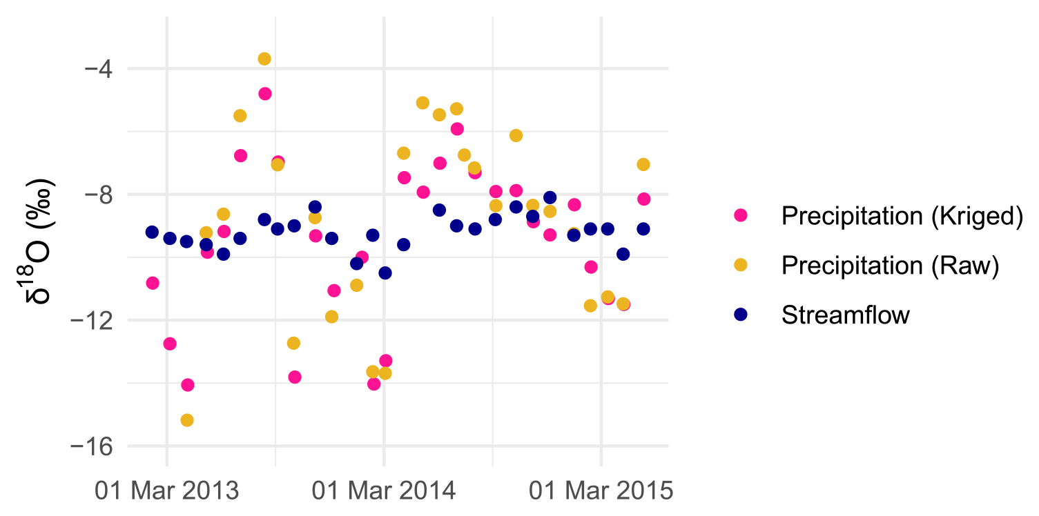
Figure 2 Data of δ¹⁸O in precipitation (kriged values as pink dots and raw values as yellow dots) and streamflow (blue dots).

3 Methods

3.1 Catchment-scale transport model

In this study, we used the tran-SAS model (Benettin and Bertuzzo, 2018a) for describing the catchment-scale water mixing and solute transport based on SAS functions. The catchment was conceptualized as a single storage S(t) (mm), whose water-age balance can be expressed as follows (Benettin and Bertuzzo, 2018a):

$$\begin{array}{}\text{(1)}& {\displaystyle }S\left(t\right)=S_{\mathrm{0}}+V\left(t\right)\text{(2)}& {\displaystyle }\begin{array}{rl}{\displaystyle \frac{\partial S_T(T,t)}{\partial t}}& +{\displaystyle \frac{\partial S_T(T,t)}{\partial T}}=P\left(t\right)-Q\left(t\right)\cdot {\mathrm{\Omega }}_Q(S_T,t)\\ & -\mathrm{ET}\left(t\right)\cdot {\mathrm{\Omega }}_{\mathrm{ET}}(S_T,t),\end{array}\text{(3)}& {\displaystyle }\text{with an initial condition of }{S}_T(T,t=\mathrm{0})=S_{T_{\mathrm{0}}}\left(T\right)\text{(4)}& {\displaystyle }\text{and a boundary condition of }{S}_T(\mathrm{0},t)=\mathrm{0}.\end{array}$$

Here, S₀ (mm) is the initial storage; V(t) (mm) represents the storage variations; P(t) (mm d⁻¹), Q(t) (mm d⁻¹), and ET(t) (mm d⁻¹) are precipitation, discharge, and evapotranspiration, respectively; S_T(T,t) (mm) is the age-ranked storage; $S_{T_{\mathrm{0}}}\left(T\right)$ (mm) is the initial age-ranked storage; and Ω_Q(S_T,t) (–) and Ω_ET(S_T,t) (–) are the cumulative SAS functions for Q and ET, respectively.

By definition, the TTD of streamflow p_Q(T,t) (d⁻¹) is calculated as follows (Benettin and Bertuzzo, 2018a):

$$\begin{array}{}\text{(5)}& p_Q(T,t)={\displaystyle \frac{\partial {\mathrm{\Omega }}_Q(S_T,t)}{\partial S_T}}\cdot {\displaystyle \frac{\partial S_T}{\partial T}}.\end{array}$$

The isotopic signature in streamflow C_Q(t) (‰) can be obtained as follows (Benettin and Bertuzzo, 2018a):

$$\begin{array}{}\text{(6)}& C_Q\left(t\right)=\underset{\mathrm{0}}{\overset{+\mathrm{\infty }}{\int }}{C}_{\mathrm{S}}(T,t)\cdot p_Q(T,t)\cdot \mathrm{d}T,\end{array}$$

where C_S(T,t) (‰) is the isotopic signature of a water parcel in storage. Equations (5) and (6) also apply for ET.

In this study, we tested three SAS parameterizations: the power law time-invariant (PLTI; Eq. 7, Queloz et al., 2015), power law time-variant (PLTV; Eq. 8, Benettin et al., 2017), and beta time-invariant (BETATI; Eq. 9, Drever and Hrachowitz, 2017) distributions. Here, they are expressed as probability density functions in terms of the normalized age-ranked storage P_S(T,t) (–), also known as fractional SAS functions (fSAS):

$$\begin{array}{}\text{(7)}& {\displaystyle }& {\displaystyle }\mathit{\omega }\left(P_{\mathrm{S}}\right(T,t),t)=k\cdot \left(P_{\mathrm{S}}\right(T,t){)}^{k-\mathrm{1}},\text{(8)}& {\displaystyle }& {\displaystyle }\mathit{\omega }\left(P_{\mathrm{S}}\right(T,t),t)=k\left(t\right)\cdot \left(P_{\mathrm{S}}\right(T,t){)}^{k\left(t\right)-\mathrm{1}},\text{(9)}& {\displaystyle }& {\displaystyle }\mathit{\omega }\left(P_{\mathrm{S}}\right(T,t),t)={\displaystyle \frac{\left(P_{\mathrm{S}}\right(T,t){)}^{\mathit{\alpha }-\mathrm{1}}\cdot (\mathrm{1}-P_{\mathrm{S}}(T,t){)}^{\mathit{\beta }-\mathrm{1}}}{B(\mathit{\alpha },\mathit{\beta })}}.\end{array}$$

The parameters k, α, and β determine the catchment's water-age preference for outflows, while B(α,β) is the two-parameter beta function. If k<1, or if α<1 and β>1, the system tends to discharge young water. If k>1, or if α>1 and β<1, the catchment preferably releases old water. The case of k=1 or $\mathit{\alpha }=\mathit{\beta }=\mathrm{1}$ describes no selection preference (i.e. complete water mixing). PLTV is characterized by k(t) varying linearly over time between two extremes, k₁ and k₂, as a function of the catchment wetness wi (–), i.e. $\mathrm{wi}\left(t\right)=\left(S\right(t)-S_{\min })/(S_{\max }-S_{\min })$, where S_min and S_max are the respective minimum and maximum storage values over the entire period.

3.2 Interpolation techniques for δ¹⁸O in precipitation

We tested the model with two spatial representation and two temporal interpolation methods for δ¹⁸O_P to explore the impact of input tracer data on model performance, results, and uncertainty. To evaluate the effect of spatial representation, we firstly used single-point δ¹⁸O_P measurements, which we refer to in the following as raw δ¹⁸O_P. These measurements, obtained from Lutz et al. (2018), were taken at the catchment outlet. The selection of δ¹⁸O_P at the outlet assumes a precipitation collector close to the stream gauge at the outlet, which is a common occurrence in many catchments for logistical reasons. Indeed, the outlet, where in-stream δ¹⁸O is sampled, serves as the location where all precipitation inputs across the catchment are integrated. For convenience, precipitation monitoring is also often conducted at or near the gauging station at the outlet. Secondly, we used spatially interpolated δ¹⁸O_P with kriging based on multiple locations. The spatial interpolation was conducted in Lutz et al. (2018) using raw δ¹⁸O_P from 24 precipitation collectors spread over the larger Bode region and using altitude as external drift. In a further step, the kriged δ¹⁸O_P data were weighted with spatially distributed monthly precipitation to obtain representative estimates for the study catchment. In our study, the kriged δ¹⁸O_P resulted in slightly more negative values than the raw δ¹⁸O_P from the catchment outlet (Fig. 2) because of the inclusion of more depleted δ¹⁸O_P values from locations with higher altitudes during the kriging process. By considering these two options for the spatial representation of δ¹⁸O_P, we intend to assess the influence of spatial variability and uncertainty in the simulated outputs between two opposing cases i.e. raw isotopes representing the simplest approach and kriged isotopes derived from a more sophisticated method. While there are other possibilities for the spatial representation of δ¹⁸O_P, our choice allows us to effectively address our research question regarding the effects on SAS models of tracer data in precipitation collected at a single location within the catchment or spatially interpolated from multiple sites.

SAS model results are sensitive to the choice of the temporal resolution of input tracer data, and a finer resolution is generally recommended to achieve a satisfactory level of detail (Benettin and Bertuzzo, 2018a). Additionally, a forward Euler scheme was employed to solve Eq. (2), whose precision increases with high-frequency time steps. For these reasons, we reconstructed daily δ¹⁸O_P estimates from monthly values with two interpolation schemes. First, we used a step function in which the values between two consecutive samples assumed the value of the last sample. Second, we used a sine interpolation due to the fact that δ¹⁸O_P samples typically exhibit pronounced seasonal variations with more depleted values in winter than in summer (Fig. 2). The sine-wave function has been used in several studies to describe temporal variation in δ¹⁸O_P (McGuire and McDonnel, 2006; Feng et al., 2009; Allen et al., 2019). The seasonal pattern of δ¹⁸O_P values over a period of 1 year can be described as follows (Kirchner, 2016):

$$\begin{array}{}\text{(10)}& {{\mathit{\delta }}^{\mathrm{18}}\mathrm{O}}_P\left(t\right)=a_P\cdot \cos (\mathrm{2}\cdot \mathit{\pi }\cdot f\cdot t)+b_P\cdot \sin (\mathrm{2}\cdot \mathit{\pi }\cdot f\cdot t)+k_P,\end{array}$$

where a and b are regression coefficients (–), t is the time (decimal years), f is the frequency (yr⁻¹), and k is the vertical offset of the isotope signal (‰). The coefficients a and b were estimated by fitting Eq. (10) to monthly δ¹⁸O_P values using the iteratively re-weighted least-squares (IRLS) estimation (von Freyberg et al., 2018). In our study, we reproduced the daily frequency isotopic data through the estimated regression coefficients of Eq. (10). Figure 3 displays the daily kriged and raw δ¹⁸O_P values simulated via step function and sine interpolation; by employing step function and sine interpolation as techniques to reconstruct tracer data in precipitation, we aim to analyze the effects on SAS-based results from two relatively simple, rather opposing approaches: one focusing on individual measurements and the other on seasonality.

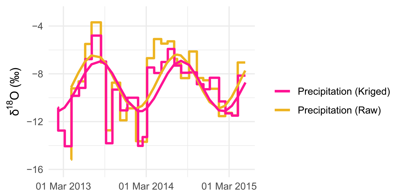
Figure 3 Predicted δ¹⁸O in precipitation (kriged values as pink lines and raw values as yellow lines) via step function and sine interpolation.

3.3 Experimental design

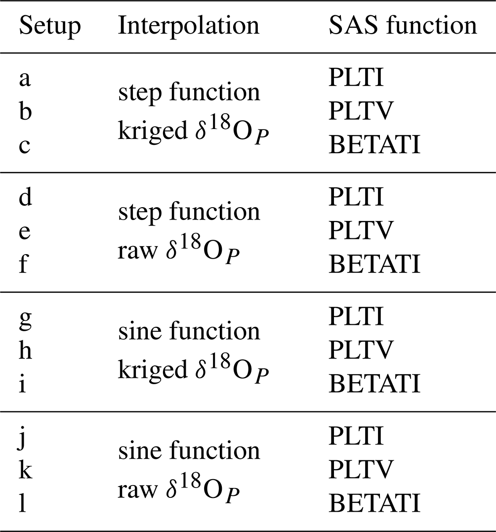
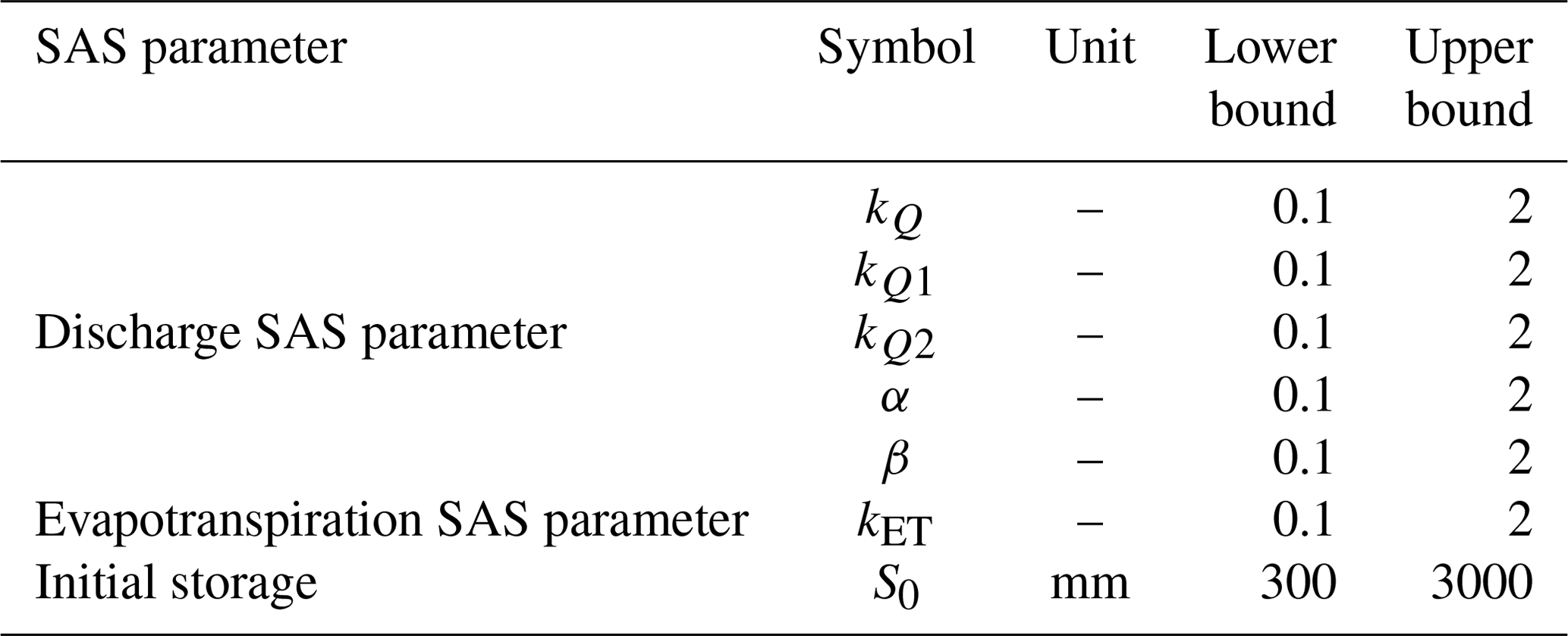
In this study, different scenarios were used to quantify uncertainty in the modeled results. We tested 12 setups composed of three SAS functions (PLTI, PLTV, and BETATI), two temporal interpolations (step and sine function), and two spatial representations (raw and kriged values) of δ¹⁸O_P (Table 1). For each setup, we performed a Monte Carlo experiment by running the model with 10 000 parameter sets generated by Latin hypercube sampling (LHS; McKay et al., 1979). Model parameters and their search ranges are shown in Table 2. A 5-year warm-up period (i.e. repetition of the input data) from February 2008 to January 2013 was performed to reduce the impact of model initialization. The period from February 2013 to May 2015 was used to infer behavioral parameters (i.e. parameter sets giving acceptable predictions) and, subsequently, to interpret model results. The initial concentration of δ¹⁸O in storage was set to 9.2 ‰, coinciding with the mean δ¹⁸O_Q over the study period.

Table 1 List of model setups.

Table 2 Model parameters and search ranges.

The informal likelihood of the Sequential Uncertainty Fitting (SUFI-2; Abbaspour et al., 2004) procedure was applied to account for uncertainty in the parameter sets and resulting modeled estimates. In SUFI-2, the uncertainty is represented by a uniform distribution, which is gradually reduced until a specific criterion is reached. In our study, we calibrated the values of model parameters until the predicted output matched the measured δ¹⁸O_Q to a satisfactory level, defined by an objective function. As the objective function, we employed the Kling–Gupta efficiency (KGE; Gupta et al., 2009), and once the criterion of KGE ≥ 0.5 was satisfied, we defined a set of behavioral solutions for each model setup. However, as the aim of this study is to investigate the impact of various sources of uncertainty on simulated outputs, rather than to determine the best model setup, we decided to set a fixed sample size and narrow down those solutions generated by SUFI-2 in the previous step. Setting a fixed sample size ensures the comparability of results across the setups, as different sample sizes could influence the uncertainty analysis (i.e. the greater the number of behavioral solutions, the wider the uncertainty band). By fixing the sample size, we can still meet the requirement of a minimum acceptable KGE value (i.e. KGE ≥ 0.5). In this study, we determined the final behavioral solutions by using a fixed sample size that corresponds to the best 5 % parameter sets and modeled results in terms of the KGE.

To assess the range of possible behavioral solutions and understand the level of uncertainty associated with it, we calculated the 95 % confidence interval (CI) derived by computing the 2.5 % and 97.5 % percentile values of the cumulative distribution in the parameters and time series of output variables (Abbaspour et al., 2004). These percentile values represent the lower and upper bounds of the CI, respectively. In our experimental setup, the main output variables were the in-stream δ¹⁸O signature and backward median transit time (TT₅₀, in days, i.e. the time it takes for half of the water particles to leave the system as streamflow at the catchment outlet). Time series of TT₅₀ were extracted directly from daily TTDs (Eq. 5) and used as a metric for the streamflow age. This was done because TTDs are typically skewed with long tails (Kirchner et al., 2001); hence, the median is often a more suitable metric than, for example, the MTT, as it is less impacted by the poor identifiability of the older water components (Benettin et al., 2017).

4 Results

4.1 Simulated δ¹⁸O in streamflow and model performance

Modeled δ¹⁸O values in streamflow (δ¹⁸O_Q) represented by the 95 % confidence interval (CI) in the ensemble solution are displayed in Fig. 4. The results reveal how the predicted δ¹⁸O_Q values enveloped the measured isotopic signature by reproducing its seasonal fluctuations, with depleted (i.e. more negative) values in winter and enriched (i.e. less negative) values in summer. Although the behavioral parameter sets were able to capture the seasonal isotopic trend, they poorly reproduced the exact values; therefore, the ensemble simulations are characterized by a non-negligible uncertainty.

Figure 4 shows the distinct effects of the interpolated input tracer data and model parameterization on the simulated δ¹⁸O_Q values. The step function interpolation generated an erratic isotopic signature in streamflow with flashy fluctuations (Fig. 4a–f). On the other hand, sine interpolation of δ¹⁸O_P values yielded a smooth response in the simulated δ¹⁸O_Q values (Fig. 4g–l). No significant visual distinction was found between kriged (Fig. 4a–c) and raw (Fig. 4d–f) δ¹⁸O_P samples when the step function interpolation was used, except for a slightly larger uncertainty observed with raw δ¹⁸O_P samples. Furthermore, when employing the sine interpolation and raw δ¹⁸O_P values (Fig. 4j–l), the simulations overestimated the in-stream measurements in comparison with kriged values (Fig. 4g–i). Finally, distinct SAS parameterizations did not produce remarkable differences in the simulated δ¹⁸O_Q values, although PLTV generally yielded simulations that better enveloped the measured isotopic signature (Fig. 4b, e, h, k).

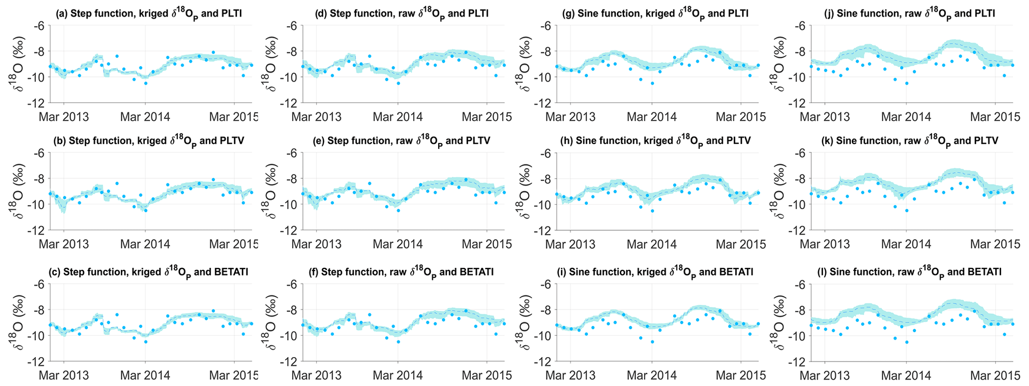
Figure 4 Predicted δ¹⁸O values in streamflow. The dark blue filled circles represent the observed data, and the dashed light blue lines and shaded areas represent the ensemble mean of all possible solutions and their range according to the 95 % CI, respectively.

Despite the differences in the predicted δ¹⁸O_Q values, all simulations can be considered satisfactory given the KGE values ranging between 0.55 and 0.72 across all tested setups (Fig. 5). This aforementioned model performance can be classified as intermediate (Thiemig et al., 2013) to good (Andersson et al., 2017; Sutanudjaja et al., 2018). When considering the best fit, the combination of step function interpolation and raw δ¹⁸O_P values performed best. Additionally, PLTV generally yielded slightly better KGE values than PLTI or BETATI when grouping the setups with the same spatiotemporal interpolation of δ¹⁸O_P. Differences in the mean KGEs were statistically insignificant (t test with p values > 0.05) only between setups a–g, c–i–k, and j–l (Table 1), as the mean KGE values were nearly identical; this largely agrees with the visual analysis (Fig. 5). Contrarily, the differences in the mean KGE values of the remaining setups were statistically significant (p values < 0.05), indicating that the a priori methodological choices (i.e. interpolation techniques of δ¹⁸O_P values and/or SAS parameterization) strongly impact the overall results. Nonetheless, this does not mean that we can clearly identify the most suitable setup, but there is a need to carefully analyze the multiple potential choices with respect to SAS parameterization and tracer data interpolations as well as to evaluate the uncertainty range in modeled predictions.

Figure 5 Box plots of model performance ranges in behavioral solutions. The letters on the x axis refer to the model setup type according to Table 1. Box plots filled with the same colors represent model setups characterized by the same interpolation scheme in space and time. On each box, the central red line indicates the median, and the bottom and top edges of the box indicate the 25th and 75th percentiles, respectively, namely the interquartile range (IQR). The whiskers extend to the most extreme data points not considered outliers, which are the 25th percentile − 1.5 × IQR and the 75th percentile + 1.5 × IQR, respectively. The outliers are plotted individually using the red “+” markers.

Ranges of the behavioral SAS parameters for the tested setups are summarized in Table S1 in the Supplement. Parameters for the SAS functions of Q (i.e. k_Q, k_Q1, k_Q2, α, and β) were different across the setups, although they were generally relatively narrow and well identified. However, the behavioral parameters were better constrained when using the step function interpolation, as their 95 % CI was, on average, 34 % narrower than that provided by the sine interpolation, across all the SAS parameterizations. The parameters k_Q1 and α were also better identified than k_Q2 and β, as their 95 % CI was, on average, 56 % narrower, across all tested setups. Conversely, there was no clear difference in the parameter ranges when using kriged or raw δ¹⁸O_P values. The evapotranspiration parameter (i.e. k_ET) was poorly identified in all setups, as any value in the search range provided equally good results. The initial storage (i.e. S₀) was only partially constrained, as any value between 335 and 2895 mm was considered acceptable.

4.2 Simulated transit times and model uncertainty

Figure 6 illustrates the 95 % CI of the behavioral solutions for the predicted median transit time (TT₅₀). The results show that the model simulated largely different ranges of TT₅₀ based on the tested setups. When using PLTI and BETATI (Fig. 6a, c, d, f, g, i, j, l), the 95 % CI was relatively stable with smaller fluctuations throughout the simulation period compared with PLTV (Fig. 6b, e, h, k). However, minor differences emerged across the simulated TT₅₀ as a result of the distinct interpolation techniques used for δ¹⁸O_P. The 95 % CI of TT₅₀ was, on average, 37 % larger, across all tested setups, when using raw δ¹⁸O_P (Fig. 6d–f and j–l) rather than kriged δ¹⁸O_P (Fig. 6a–c and g–i). This was especially visible when the step function was used (Fig. 6a–f). Moreover, the sine interpolation generated a 95 % CI of TT₅₀ that was, on average, 62 % narrower across all tested setups (Fig. 6g–l) with respect to the step function (Fig. 6a–f). These differences were more evident for high-flow conditions where the 95 % CI of TT₅₀ showed a significant reduction. In addition, the behavioral solutions obtained with the sine interpolation (Fig. 6g–l) were more skewed towards shorter mean TT₅₀ values, across all tested setups, than those of the step function (Fig. 6a–f).

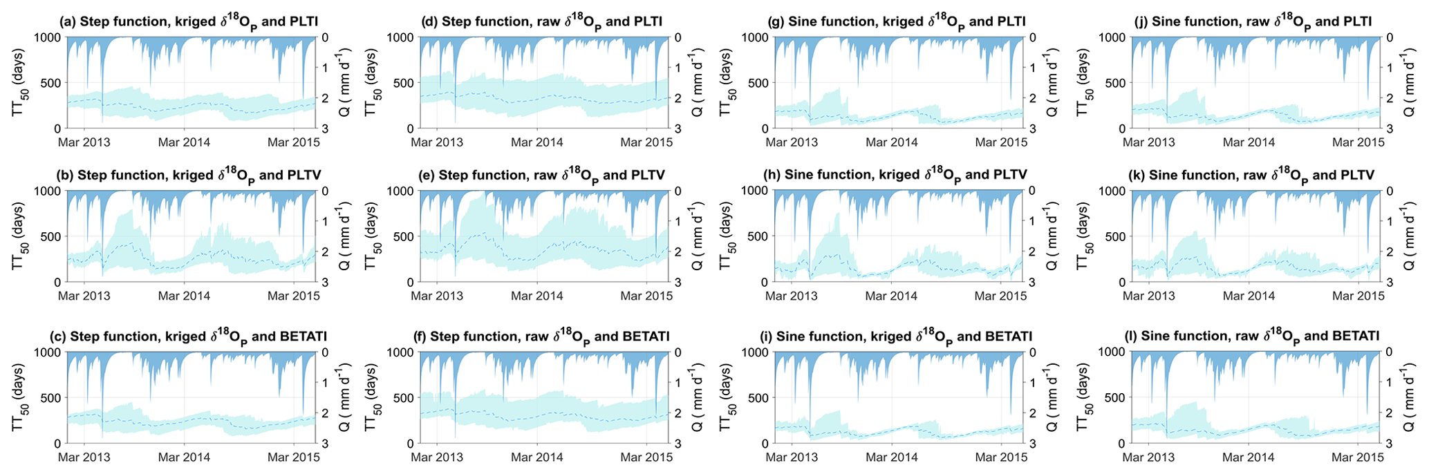
Figure 6 Predicted TT₅₀ of streamflow. The dashed light blue lines and shaded areas represent the ensemble mean of all possible solutions and their range according to the 95 % CI, respectively.

Behavioral solutions obtained with PLTV revealed a similar pattern regardless of the interpolation employed (Fig. 6b, e, h, k). Nonetheless, there was a noticeable difference in the 95 % CI of TT₅₀ under distinct flow regimes. During low flows and dry periods (i.e. summer and autumn), the time series of predicted TT₅₀ showed large uncertainties ranging at most between 259 and 1009 d across the different setups (Fig. 6e). Conversely, during high flows (i.e. winter and spring), the 95 % CI was much narrower and varied at least between 126 and 154 d (Fig. 6h). The large 95 % CI and the notable differences across the tested setups highlight the sensitivity and, in turn, the uncertainty in the predicted TT₅₀ to the model parameterization, temporal interpolation of input data, hydrologic conditions, and nonspatially interpolated δ¹⁸O_P.

In general, the variability in the predicted TT₅₀ was controlled by the hydrological state of the system (Fig. 6). High-discharge events reduced the TT₅₀ values, whereas low-flow periods were associated with a longer estimated TT₅₀. This is expected, as streamflow during high (low) flows is dominated by near-surface runoff (groundwater) with shallow (deep) flow paths leading to a shorter (longer) TT₅₀. Such differences were particularly visible with PLTV (Fig. 6b, e, h, k), as the exponent k_Q(t) shifts the water selection preference over time as a function of the wet/dry conditions. This resulted in the variability in TT₅₀ being more pronounced than that of PLTI and BETATI, whose SAS parameters for Q are constant over time.

4.3 Catchment-scale water release

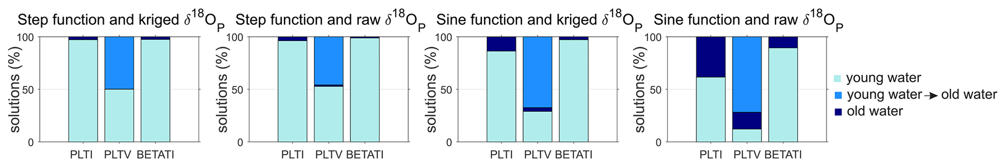
SAS functions provided valuable insights into the catchment-scale water release dynamics. Figure 7 presents the behavioral solutions releasing water of different ages and also shows that the catchment generally experienced a stronger affinity for releasing young water (i.e. k_Q<1, or α<1 and β>1), rather than old water (i.e. k_Q>1, or α>1 and β<1). These findings are in agreement with other studies in the upper Selke catchment (Winter et al., 2020; Nguyen et al., 2021). Nonetheless, there were differences in the water release scheme when comparing various combinations of SAS functions and spatiotemporal interpolation techniques of isotopes. The use of PLTV resulted in a substantial number of solutions, approximately 50 % of all behavioral solutions, suggesting a preference for both young and old water. On the other hand, only a few solutions showed affinity for old-water release, and this was more prominent when using the sine interpolation, raw δ¹⁸O_P values, and PLTI across all tested setups.

Figure 7 Percentage of behavioral solutions releasing water of different ages.

5 Discussion

5.1 Uncertainty in TTD modeling

In this study, we characterized the TTD uncertainty arising from some significant and critical aspects for the SAS modeling. These aspects are also the most directly linked to the data interpolation and SAS parameterization that we explored in this work. The uncertainty analysis was carried out across the 12 tested setups corresponding to different combinations of spatiotemporal data interpolation techniques and SAS parameterizations. Our results show that the uncertainty (i.e. 95 % CI) of the simulated TT₅₀ (Fig. 6) was firmly dependent on the choice of model setup, as the 95 % CI was primarily sensitive to the type of SAS function, temporal interpolation, and spatial representation of δ¹⁸O_P.

Uncertainty in the simulated TT₅₀ differed considerably between time-invariant (i.e. PLTI and BETATI; Fig. 6a, c, d, f, g, i, j, l) and time-variant (i.e. PLTV; Fig. 6b, e, h, k) SAS functions; thus, a large sensitivity is associated with the choice of the SAS parameterization. For example, PLTI and BETATI explicitly assume constant water selection preference over time, as these functions do not consider the temporal variability in the catchment wetness. As a consequence, the resulting TT₅₀ had a moderately stable 95 % CI with smaller fluctuations compared with those of PLTV. On the other hand, including an explicit time dependence in the SAS function strongly affected the 95 % CI of TT₅₀. Notably, PLTV produced a wider 95 % CI during low-flow conditions, which can hinder the TTDs ability to provide robust insights into flow and solute transport behaviors in the study area during low-flow conditions. This highlights the need to further constrain PLTV with additional data, which could involve obtaining tracer data at a finer resolution or additional information on the evapotranspiration and initial storage. In addition, the exceptionally old flow components associated with a very large 95 % CI of TT₅₀ might be a distortion of the actual TT₅₀ values, which can usually be more reliably estimated using radioactive tracers than with stable isotopes (Visser et al., 2019). Hence, PLTV-based TT₅₀ greater than the observed period (828 d) should be interpreted carefully. It is important to note that we discussed the fractional SAS (fSAS) functions in this study, but another form of the SAS functions, such as the rank SAS (rSAS) functions, may have different uncertainty. This is mainly due to the difference in how the storage is considered: fSAS functions are expressed as function of the normalized age-ranked storage, which is equal to the cumulative residence time, whereas rSAS functions depend on the age-ranked storage, which is the volume of water in storage ranked from youngest to oldest (Harman, 2015).

Likewise, the high-frequency reconstruction of δ¹⁸O_P from monthly samples via interpolation created further uncertainty. The sine interpolation effectively captured the dominant features of the observed δ¹⁸O_P, such as seasonality. Consequently, sine interpolation successfully reproduced the seasonal trend in in-stream δ¹⁸O, although simulations overestimated the measurements (Fig. 4g–l). On the other hand, sine interpolation poorly reproduced rainfall isotopes during short-term flashy events and missed detailed characteristics of the tracer dataset by smoothing the variability in the observed δ¹⁸O_P (Fig. 3). As a result, high values of δ¹⁸O_P are underestimated, whereas low values are overestimated. It is critical to recognize these limitations when interpreting modeling results, as uncertainty in the simulated δ¹⁸O_P may conceal a more pronounced hydrological response of the system (Dunn et al., 2008; Birkel et al., 2010; Hrachowitz et al., 2011). Contrarily, step function interpolation preserved the maxima in the monthly observed δ¹⁸O_P values by capturing their variation correctly (Fig. 3). Simulations showed a better fit with measured in-stream δ¹⁸O (Fig. 4a–f) and higher model performance (Fig. 5). However, combining step function with raw δ¹⁸O_P resulted in larger uncertainty in the simulated TT₅₀ (Fig. 6d–f). This reflects the need for a comprehensive exploration of the uncertainty range, rather than relying solely on the goodness of fit. Overall, the choice between step function and sine interpolation largely affected the reconstructed input data (Fig. 3), leading to significant differences in the simulated TT₅₀ and associated uncertainty. It is important to note that alternative methods, such as generalized additive models (GAMs; Buzacott et al., 2020), offer other options for interpolating tracer data. We conducted further tests with the SAS model using a GAM to reconstruct both kriged and raw δ¹⁸O_P using smoothing functions; this provides a more sophisticated approach than the intuitive methods used in this study. However, the results, available in the Supplement, show that while a GAM provided more detailed reconstructed input tracer data (Fig. S1), it did not significantly alter the SAS-based results (Figs. S2, S3) or yield any new insights or conclusions about uncertainty with respect to using step function and sine interpolation. Therefore, we conclude that, while highly resolved input data may seem appealing, they do not necessarily lead to substantial benefits for the SAS-based output, supposedly due to the conceptual simplifications in the SAS model.

The spatial representation of δ¹⁸O_P values had limited impact on the overall pattern of simulated TT₅₀, as the time series were comparable with both kriged (Fig. 6a–c and g–i) and raw (Fig. 6d–f and j–l) δ¹⁸O_P. Nonetheless, the spatial interpolation of δ¹⁸O_P from different locations resulted in a reduction in the uncertainty in the TT₅₀, which was particularly evident with the step function (Fig. 6a–f). This difference may be attributed to the fact that the upper Selke is a large (mesoscale) catchment with a substantial gradient in elevation, and, as a consequence, measurement for δ¹⁸O_P from only one location may be generally overly simplistic. This finding highlights the importance of considering not only the model performance (Fig. 5; raw values with a step function interpolation produced higher KGE values) but also the uncertainty range in predicted TT₅₀.

Finally, we found that the uncertainty was larger under dry conditions when lower flow and longer TT₅₀ were observed. This was especially visible when using the time-variant SAS function (Fig. 6b, e, h, k). It might be due to the fact that, under wet conditions, there is a high level of hydrologic connectivity within the catchment (Ambroise, 2004; Blume and van Meerveld, 2015; Hrachowitz et al., 2016), which results in nearly all flow paths being active and contributing to the streamflow. This, ultimately, may make TT₅₀ values easier to constrain. Conversely, under dry conditions, when usually only longer flow paths carrying older water are active (Soulsby and Tetzlaff, 2008; Jasechko et al., 2017), water partially flows through a drier soil zone where flow is more erratic (i.e. flow directions and patterns can vary widely) as the conductivity is controlled by soil moisture. As a result, wet areas can be patchy and water flows preferentially at certain locations only, as opposed to spatially uniform flow through the soil matrix; this might make it more challenging to constrain older water ages. Similarly, Benettin et al. (2017) found higher uncertainty in the simulated SAS-based median water ages during drier periods, potentially due to higher uncertainty in the total storage. Moreover, non-SAS function studies have observed major uncertainties and deviations from observations in lumped modeled results during low-flow conditions (Kumar et al., 2010). This was primarily due to the lack of spatial variability in the catchment characteristics in lumped models, which is a critical factor controlling low-flow regimes in rivers.

The dissimilarities in the simulated TT₅₀ across the tested setups underline the importance of accounting for uncertainty in model-based TTDs. The uncertainty analysis with SUFI-2 performed in this study was essential to best describe the parameter identifiability and bounds of the behavioral solutions of each output variable. Furthermore, our results highlight the importance of gaining tracer datasets of good quality (i.e. tracer data with a finer temporal resolution), considering the spatial variability in the isotopic composition in precipitation, and, possibly, employing a model parameterization that best describes the catchment-specific storage and release dynamics. The last point can be defined according to a precise conceptual knowledge of the catchment’s functioning and information from previous studies in similar catchments.

5.2 TTD modeling: advantages and limitations

Our results provide visually plausible seasonal fluctuations in the predicted δ¹⁸O_Q samples (Fig. 4) and satisfactory KGE values (Fig. 5), despite the uncertainty arising from model inputs, structure, and parameters. The good match with observations provides confidence in the simulated TT₅₀ for the upper Selke catchment. The magnitude of the uncertainty resulting from different setups cannot be generalized, but the overall approach for uncertainty assessment presented here could be extended to other areas and TTD studies. However, we recognize some limitations and indicate below possible reasons and, in turn, improvements that future work could achieve.

First, the limited length of the δ¹⁸O time series might not describe the system accurately; hence, implementing longer time series could improve the parameter identifiability and provide a more accurate estimation of the TTDs. Second, this study relied on stable water isotopes, which might underestimate the tails of the TTDs (Stewart et al., 2010; Seeger and Weiler, 2014), although recent works have contested this (Wang et al., 2022). Possible advancements could be reached by using decaying tracers varying over a longer timescale than stable water isotopes (e.g. tritium; Stewart et al., 2012; Morgenstern et al., 2015) and imparting more information on old water. Next, future work should retrieve more information on the evapotranspiration ET and initial storage S₀, whose parameters were poorly identified. However, this issue is common in transport studies that rely on measurements of in-stream stable water isotopes (Benettin et al., 2017; Buzacott et al., 2020). As a way forward, information on the ET isotopic compositions might help better constrain ET parameters and assess their affinity for young/old water. Regarding constraining the range of S₀, further information can be gained from geophysical surveys in the study areas or groundwater modeling as well as by using decaying isotopes (Visser et al., 2019).

5.3 Implications of TTD uncertainties

This study characterized the uncertainty in TTDs, which summarize the catchment's hydrologic transport behavior and, therefore, comprise decisive information for water managers. The value of TT₅₀ has relevant implications for both water quantity and quality, as does its uncertainty. The larger the 95 % CI in the simulated TT₅₀, the greater the difference in the TT₅₀ values, which, ultimately, implies distinct hydrological processes, water availability, groundwater recharge, and solute export dynamics (McDonnel et al., 2010).

For example, knowing the TTD and its uncertainty may be crucial for characterizing the catchment's response to climatic change (Wilusz et al., 2017). Considering the increasing severity of droughts in the past decades (Dai, 2013), a catchment with a shorter TT₅₀ and a dominant release of young water might be more affected by droughts than a catchment with a longer TT₅₀, which means that its stream is fed by relatively old water sources. Therefore, a short TT₅₀ reveals a low drought resilience of the catchment and limited water availability, which could limit streamflow generation processes and change the in-stream water quality status during drought periods (Winter et al., 2023). Likewise, TTD uncertainty may affect the understanding of the water infiltration rate, hydrological processes, and aquifer recharge, as a shorter TT₅₀ suggests that water is quickly routed to the catchment outlet rather than infiltrating deeply into the groundwater. Finally, TTD uncertainty can have an impact on the quantification of the modern groundwater age, i.e. groundwater younger than 50 years (Bethke and Johnson, 2008). According to Jasechko (2019), the correct identification of modern groundwater abundance and distribution can help determine its renewal (Le Gal La Salle et al., 2001; Huang et al., 2017), groundwater wells and depths most likely to contain contaminants (Visser et al., 2013; Opazo et al., 2016), and the part of the aquifer flushed more rapidly.

Uncertainty in TTDs also impacts on assessing the fate of dissolved solutes, such as nitrates (X. Yang et al., 2018; Nguyen et al., 2021, 2022; Lutz et al., 2022), pesticides (Holvoet et al., 2007; Lutz et al., 2017), and chlorides (Kirchner et al., 2000; Benettin et al., 2013). These solutes constitute a crucial source of diffuse water pollution in agricultural areas (Jiang et al., 2014; Kumar et al., 2020), as they are spread on the soil in large quantities, especially during the growing season. The exposure time of solutes with the soil matrix has strong consequences for biogeochemical reactions, such as denitrification in the case of nitrates (Kolbe et al., 2019; Kumar et al., 2020). A short TT₅₀ suggests that water can be rapidly conveyed to the stream network (Kirchner et al., 2001), with limited time for denitrification. This explains the elevated in-stream concentration and short-term impact of nitrate export compared with that of a longer TT₅₀, which is typically associated with old-water release and a low nitrate concentration (Nguyen et al., 2021). Similarly, pesticide transport is highly affected by the TTD uncertainty, as a long TT₅₀ suggests little pesticide degradation due to decreased microbial activity along deeper flow paths (Rodríguez-Cruz et al., 2006). In other cases, a shorter TT₅₀ may limit the time for degradation, causing a peak in the in-stream concentration (Leu et al., 2004). Overall, a longer TT₅₀ can delay or buffer the catchment's reactive solute response at the outlet (Dupas et al., 2016; Van Meter et al., 2017). This creates a long-term effect of hydrological legacies and a continuous problem with diffuse pollution of nitrates (Ehrhardt et al., 2019; Winter et al., 2020) and pesticides (Lutz et al., 2013), which can persist in the catchment for several years. Finally, TTD uncertainties also play an important role in chloride transport, although chlorides are commonly known to be conservative (Svensson et al., 2012). A short TT₅₀ may indicate rapid chloride mobilization, whereas a long TT₅₀ implies chloride persistence in groundwater; therefore, chloride accumulates and is released at lower rates, with impacts on the ecosystem functions, vegetation uptake, and metabolism (Xu et al., 1999).

Understanding the uncertainty in TTDs is crucial for the aforementioned implications. While previous studies have used only a specific SAS function and/or specific tracer data interpolation technique in time and space, here we show that there could be a wide range of different results in terms of water ages, model performance, and parameter uncertainty. This is due to the specific choice regarding SAS parameterization and tracer data interpolation. With this, we want to convey that uncertainty is omnipresent in TTD-based models, and we need to recognize it, especially when dealing with sparse tracer data and multiple choices for model parameterization. Therefore, we want to encourage future studies to explore these uncertainties in other catchments and different geophysical settings, with the final aim to investigate whether these uncertainties may affect the conclusions of water quantity and quality studies for management purposes.

6 Conclusions

This study explored the uncertainty in TTDs of streamflow, resulting from 12 model setups obtained from different SAS parameterizations (i.e. PLTI, PLTV, and BETATI), and reconstruction of the precipitation isotopic signature in time and space via interpolation (step function vs. sine fit and raw vs. kriged values).

We found satisfactory KGE values, whose differences across the tested setups were statistically significant, meaning that the choice of the setup matters. As a consequence, distinct setups led to considerably different simulated TT₅₀ values. The choice between using time-variant or time-invariant SAS functions was crucial, as the time-invariant functions generated moderate fluctuations in the 95 % CI of the estimated TT₅₀ because of the constant water selection preference over time. On the other hand, the time-variant SAS function captured the dynamics of the catchment wetness, resulting in more pronounced fluctuations in TT₅₀. However, the time-variant SAS function also produced a larger 95 % CI in TT₅₀, notably during drier periods, which might indicate the need to constrain the function with additional data (e.g. finer tracer data resolution and/or information on evapotranspiration and storage). Significant differences in TT₅₀ were observed depending on the employed temporal interpolations. Results from the sine interpolation produced a smaller uncertainty in TT₅₀, with the time series skewed towards smaller values. However, such results must be interpreted carefully, as the sine interpolation poorly reproduced flashy events in precipitation, thus indicating that some more dynamic transport processes were not fully considered. Conversely, the step function interpolation resulted in a larger uncertainty in the TT₅₀, but it was able to better reproduce the measured δ¹⁸O_P data by capturing the peak values, as opposed to the sine interpolation. Dry conditions were another reason for uncertainty, as indicated by the high variance in the simulated TT₅₀ values, which is potentially attributed to the water preferentially moving at certain locations, making wet areas patchy, so it may be more challenging to accurately constrain older water ages. Finally, there was comparable pattern in the modeled results when using kriged vs. raw isotopes, but the kriged values yielded an uncertainty reduction in TT₅₀. This highlights the potential advantage of spatially interpolated values over a single measurement representative of the entire area, particularly in a mesoscale catchment that varies with respect to elevation.

These findings provide new insights into TTD uncertainty when high-frequency tracer data are missing and the SAS framework is used. Regardless of the degree of efficiency or uncertainty, the decision on which setup is more plausible depends on the best conceptual knowledge of the catchment functioning. We consider the presented approach to be potentially applicable to other studies to enable a better characterization of TTD uncertainty, improve TTD simulations and, ultimately, inform water management. These aspects are particularly crucial in view of increasingly extreme climatic conditions and worsening water pollution under global change.