Bayesian parameter inference in hydrological modelling using a Hamiltonian Monte Carlo approach with a stochastic rain model

Stochastic models in hydrology are very useful and widespread tools for making reliable probabilistic predictions. However, such models are only accurate at making predictions if model parameters are first of all calibrated to measured data in a consistent framework such as the Bayesian one, in which knowledge about model parameters is described through probability distributions. Unfortunately, Bayesian parameter calibration, a. k. a. inference, with stochastic models, is often a computationally intractable problem with traditional inference algorithms, such as the Metropolis algorithm, due to the expensive likelihood functions. Therefore, the prohibitive computational cost is often overcome by employing over-simplified error models, which leads to biased parameter estimates and unreliable predictions. However, thanks to recent advancements in algorithms and computing power, fully fledged Bayesian inference with stochastic models is no longer off-limits for hydrological applications. Our goal in this work is to demonstrate that a computationally efficient Hamiltonian Monte Carlo algorithm with a timescale separation makes Bayesian parameter inference with stochastic models feasible. Hydrology can potentially take great advantage of this powerful data-driven inference method as a sound calibration of model parameters is essential for making robust probabilistic predictions, which can certainly be useful in planning and policy-making. We demonstrate the Hamiltonian Monte Carlo approach by detailing a case study from urban hydrology. Discussing specific hydrological models or systems is outside the scope of our present work and will be the focus of further studies.

1 Introduction

A fundamental and highly non-trivial question in many applied sciences is how to make reliable predictions about the dynamics of a complex system. In hydrological modelling in particular, the ability of predicting extreme events like floods is obviously of paramount importance. Conceptual rainfall-runoff models that incorporate only a few state variables and a few system parameters often represent a very practical and efficient solution for making probabilistic predictions. The basic idea is to describe slow processes occurring at our observation scale by phenomenological differential equations and include all other processes as noise. Incorporating the noise in the model, where it arises, naturally leads to stochastic differential equation (SDE) models. Model parameters then need to be calibrated on observed data, usually provided in the form of noisy time series. The goal of the calibration process is to determine the parameters that allow the model to reproduce the observed data and quantify their uncertainties, expressed as probability distributions. For this purpose, Bayesian statistics is a consistent framework where our knowledge about model parameters is described by probability distributions and learning as a data-driven updating process of prior beliefs. Bayesian inference methods bear the great advantage over traditional optimization algorithms of providing an uncertainty estimation for the calibrated parameters in the form of a probability distribution. The knowledge of such uncertainty is important for making probabilistic predictions, which can in turn be a useful tool for decision-makers. Hydrology could potentially take great advantage of more realistic stochastic models and a fast and reliable method for their calibration. However, Bayesian inference turns out to be computationally very expensive for non-trivial stochastic models.

Uncertainty in rainfall-runoff hydrological modelling arises mostly from input errors associated with an inaccurate estimation of the integrated rainfall over a catchment (Kavetski et al., 2006). These input errors, typically due to a combination of heterogeneous rainfall, sparse rain-gauge measurements and insufficient temporal resolution (McMillan et al., 2011; Renard et al., 2011; Ochoa-Rodriguez et al., 2015), can seriously deteriorate the quality of model calibration results for heavily input-driven hydrological systems (Bárdossy and Das, 2008). A variety of stochastic weather generators (Rodriguez-Iturbe et al., 1987; Cowpertwait et al., 1996; Deidda et al., 1999; Paschalis et al., 2013; Langousis and Kaleris, 2014) have been proposed to simulate precipitation with its uncertainty. Although such weather generators can provide uncertain inputs to rainfall-runoff models and therefore reproduce the effect of rainfall errors on runoff predictive uncertainties, such input uncertainties have been largely neglected in studies focusing on model parameter inference (Sikorska et al., 2012), probably because of the computational difficulty of including them in a likelihood function (Honti et al., 2013). Input uncertainties should be included directly in the input as a stochastic contribution and then transported through the model and thereby naturally incorporated in the likelihood function describing the probability distribution of observations given model parameters. In the Bayesian framework, the sought posterior probability distribution for the model parameters is proportional to the product of the likelihood function and the prior probability distribution describing our prior knowledge about model parameters. However, it is still common practice in hydrology, as well as in other applied disciplines, to consider an over-simplified error model based on likelihood functions defined as uncorrelated normal distributions centred on the outputs of a deterministic model (Yang et al., 2008; Reichert and Schuwirth, 2012; Sikorska et al., 2012). This inevitably leads to biased parameters and unreliable predictions (Renard et al., 2011; Honti et al., 2013; Del Giudice et al., 2015). Although so-called rainfall multipliers can mitigate this problem (Kavetski et al., 2006; Sun and Bertrand-Krajewski, 2013), they fail in assessing input uncertainties when a rainfall event is not detected by the available rain gauges (Kavetski et al., 2006; Renard et al., 2011).

Del Giudice et al. (2016) proposed a method based on an input uncertainty model describing the rainfall as a continuous stochastic process. The method is called SIP (acronym for stochastic input process). The idea of describing selected model parameters or inputs as stochastic time-dependent processes in order to take intrinsic uncertainties realistically into account in hydrological modelling has gained momentum in recent years (Tomassini et al., 2009; Reichert and Mieleitner, 2009; Reichert et al., 2021; Bacci et al., 2022). The SIP technique uses (i) possibly inaccurate rain-gauge precipitation data, (ii) runoff data from a flowmeter at the catchment outlet, (iii) a hydrological runoff model, (iv) a rainfall model in the form of a transformed stochastic Ornstein–Uhlenbeck (OU) process, (v) models for rainfall and runoff observation errors, and (vi) prior distributions, to infer both the marginal posterior distributions for the parameters of interest and a “true” spatially integrated average rainfall over the catchment in a Bayesian manner. The SIP method uses the catchment as an additional rain gauge to gather information about a catchment-averaged real rain, which is inferred from both prior knowledge and observations of rainfall and runoff. Both the hydrological model describing the catchment dynamics and runoff observations are assumed to be accurate in comparison to the rainfall data. The inferred rainfall pattern can then be used to calibrate the model and significantly reduce the bias in the estimated parameters, despite the inaccuracy of the rainfall data. However, as described in detail in Del Giudice et al. (2016), the likelihood function turns out to be a high-dimensional discretized version of an infinite-dimensional path integral that makes this approach computationally demanding.

In Albert et al. (2016) we presented an efficient Hamiltonian Monte Carlo (HMC)-based algorithm for the calibration of SDE models on noisy time series. The proposed HMC method, combining molecular dynamics principles with the well-known Metropolis algorithm, relies on the reinterpretation of the Bayesian posterior probability distribution as the partition function of a statistical mechanics system. This interpretation reduces the parameter inference problem to the task of simulating the dynamics of a fictitious statistical mechanics system, which can be solved in a computationally efficient way. The dynamics of the statistical mechanics system may occur on very different timescales, which can be exploited by a multiple timescale integration approach. In Albert et al. (2016), the method was demonstrated using a simple, albeit general, rainfall-runoff toy model, and we claimed that the HMC algorithm, combined with the multiple timescale integration, would be applicable to a wide range of inference problems, making many SDE models amenable to a consistent Bayesian parameter inference.

Here we combine the HMC and SIP methods to perform Bayesian inference with a stochastic input model. We show that the HMC method can be extended from the toy model and the smooth synthetic data used in Albert et al. (2016) to a real-world hydrological case study with real noisy rainfall and runoff time series, albeit at the cost of a somewhat substantial analytical effort. We intentionally use sparse and inaccurate precipitation data, provided by a rain gauge located far away from the catchment area, to demonstrate that a “true” average rainfall pattern can be reconstructed from the corresponding runoff data, and we compare the inferred rain to the more accurate observations obtained from rain gauges within or very close to the catchment.

The HMC method bears valuable advantages with regard to both generality and efficiency. Indeed, it is by no means limited to an OU process, unlike the original SIP approach of Del Giudice et al. (2016), which strictly requires a linear stochastic process as a rain generator. Although in this study we also opt for an OU process for the sake of simplicity, it should be clear that such a process could be arbitrarily replaced by any other stochastic process, thus giving the method significantly more flexibility in reproducing the statistical properties of real rainfall. The HMC method is also not at all limited to urban hydrology and could be applied for instance in natural catchment hydrology as well. The specific case study presented here was chosen to put emphasis on input uncertainties, which often represent the biggest source of uncertainty in hydrological modelling in general. More information on possible hydrological applications can be found in Del Giudice et al. (2016). Moreover, the HMC algorithm allows us to sample both model parameters and a true averaged rainfall pattern that are simultaneously compatible with data, models and prior distributions from the posterior probability density. This yields very high acceptance rates, even in the context of expensive high-dimensional problems, with great benefits in terms of performance and efficiency of the algorithm. Another interesting method from the family of particle filters to tackle high-dimensional inference problems for stochastic model calibration is particle Markov chain Monte Carlo (PMCMC) (Andrieu et al., 2010), which combines piece-wise forward simulations of the stochastic model with data-based importance sampling. Like HMC, PMCMC methods can be applied to any stochastic process, including (unlike HMC) processes with discrete states (e.g. numbers of organisms in ecological models). A generally low implementation effort could be an additional argument in favour of PMCMC algorithms, which do not require the differentiation of the posterior distribution like HMC methods. However, PMCMC methods may suffer significantly in terms of efficiency when compared to an HMC-based approach. A detailed comparison, based on the same case study presented here, of different methods for Bayesian inference with stochastic models, can be found in Bacci et al. (2023). The HMC approach is very general and suitable for a broad range of applications requiring Bayesian inference with stochastic models. It should be noted that the method presented here is meant for offline-calibration of stochastic models, not for real-time updating, which might be needed in a model-based control setting. For the latter problem, filtering algorithms might be more appropriate, but we do not discuss this topic here. Moreover, HMC is inherently a MCMC method, and it is therefore embarrassingly parallelizable by breaking it up into an arbitrary number of independent Markov chains. This makes HMC very well suited for applications in the big-data regime or with expensive models.

2 Bayesian inference with a stochastic rain model

The SIP method of Del Giudice et al. (2016) describes the rain input to a hydrological system based on an unobserved and continuous stochastic process, the rainfall potential ξ(t). The latter should not be interpreted as a potential in the physical sense but rather as a rain generator based on a latent, i.e. “potential”, stochastic process that can be transformed into real precipitation P by a suitable empirical transformation P(t)=r(ξ(t)), which will be addressed below in Sect. 2.1.

The inference process allows us to learn from noisy rainfall and runoff time series, P_obs and Q_obs, respectively; the parameters θ of the hydrological system; the uncertainties σ_ξ and σ_z of both rainfall and runoff observation models, respectively; and the unobserved true rainfall over the catchment expressed as a discretized rainfall potential ξ={ξ_i}, to be interpreted as an evaluation of the stochastic process ξ(t) at a discrete set of time points t_i, with i=1, …, N.

For this purpose, we subdivide each interval between consecutive rain observations into j_P bins, yielding a total of $n_P{j}_P+\mathrm{1}=N$ discretization points, where n_P+1 is the number of rain observations, that is, the length of the precipitation time series P_obs. Analogously, the system output dimension is discretized by partitioning the intervals between consecutive runoff observations into j_Q sub-intervals, such that the total number of discretization points is $n_Q{j}_Q+\mathrm{1}=N$, where n_Q+1 is the number of data points in Q_obs. The number of discretization points is thus the same (N) in both rainfall and runoff dimensions, and it defines the discretization time step $\mathrm{d}t=T/(N-\mathrm{1})$, where T is the total time interval covered by observations. We will provide numerical values for all these constants later in Sect. 4. Here, suffice it to say that the only important requirement of the method is that the total number N of discretization points is large enough compared to the number of measurement points, n_P and n_Q, in order to accurately probe the fine dynamics occurring on short timescales between observations. Other features, such as for instance having the same number N of discretization points for rainfall and runoffs, are just arbitrary choices to ease the practical implementation of the method, which could be removed without altering the results and conclusions of this work. The same holds if the observations were irregularly spaced in time, in which case one could use observation windows with more/less intermediate discretization points. Note that a large number of discretization points N, with a fixed number of observation points, does only moderately increase the computational effort of the algorithm, since the part of the Hamiltonian dynamics that scales with N can be calculated analytically, as shown below.

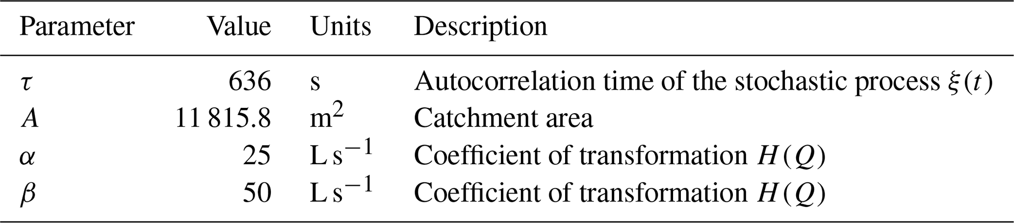
Table 1 List of model parameters that are assumed to be known, with their values and units.

The inference goal is to sample both parameter combinations (θ, σ_ξ, σ_z) and realizations ξ of the stochastic process ξ(t) from a posterior distribution obeying Bayes' equation, which reads in its discretized form as

$$\begin{array}{}\text{(1)}& \begin{array}{rl}f& \left(\mathit{\xi },\mathit{\theta },{\mathit{\sigma }}_{\mathit{\xi }},{\mathit{\sigma }}_z\mid {\mathit{P}}_{\mathrm{obs}},{\mathit{Q}}_{\mathrm{obs}}\right)\propto f\left({\mathit{Q}}_{\mathrm{obs}}\mid \mathit{\xi },\mathit{\theta },{\mathit{\sigma }}_z\right)\\ & f\left({\mathit{P}}_{\mathrm{obs}}\mid \mathit{\xi },{\mathit{\sigma }}_{\mathit{\xi }}\right)f\left(\mathit{\xi }\right)f\left(\mathit{\theta },{\mathit{\sigma }}_{\mathit{\xi }},{\mathit{\sigma }}_z\right),\end{array}\end{array}$$

where f(θ, σ_ξ, σ_z) is the joint prior distribution for the model parameters, and f(Q_obs∣ξ, θ, σ_z)f(P_obs∣ξ, σ_ξ) is the likelihood expressing the probability of observed data (P_obs, Q_obs) given model parameters (θ, σ_ξ, σ_y) and a system realization ξ, weighted by the prior probability density f(ξ).

The stochastic process realization ξ in Eq. (1) is a time series of length N≫1. The high dimensionality of the problem renders the likelihood computationally expensive, thus making the inference problem intractable with traditional Bayesian inference algorithms, such as random walk Metropolis algorithms, which require a large number of likelihood evaluations.

On the other hand, when the inference target is only the posterior distribution for the model parameters (θ, σ_ξ, σ_z) and model simulations are fast, one may resort to approximate Bayesian computation (ABC) algorithms (e.g. Albert et al., 2015), which approximate the parameters' posterior through repeated comparisons of model simulations with observations in terms of a low-dimensional set of summary statistics. However, here we are interested in the joint inference of model parameters and the real rainfall ξ, which makes ABC an inefficient approach.

To tackle this problem, we apply a Hamiltonian Monte Carlo (HMC) algorithm (Duane et al., 1987; Neal, 2011; Albert et al., 2016), which exploits the principles of Hamiltonian dynamics to attain very high acceptance rates and low auto-correlation, even on high-dimensional sampling spaces. This makes it possible to explore such spaces with large steps, without compromising the acceptance rate and thus making the algorithm very efficient. The inherent high efficiency of HMC is further boosted here by a timescale separation analogous to the one described in Albert et al. (2016).

The HMC algorithm allows us to sample simultaneously from the posterior of Eq. (1) both model parameters (θ, σ_ξ, σ_z) and realizations of the stochastic process ξ. In particular, the rainfall potential ξ is inferred indirectly using prior knowledge, the observed runoff Q_obs and the possibly inaccurate observed precipitation P_obs. The discharge data are used as an indirect source of knowledge about the rainfall, which complements the unreliable information due to the sparse rain-gauge measurements.

The method described here requires a stochastic input process (i.e. a rainfall model), a hydrological rainfall-runoff model to describe the observed discharges Q_obs, observation models for both rainfall and runoff, and prior probability distributions, which are all outlined below.

2.1 The rainfall model

The rainfall potential is described by a normal and linear Ornstein–Uhlenbeck (OU) process with mean zero and standard deviation unity, which can be written in the form of a Langevin equation as

$$\begin{array}{}\text{(2)}& \dot{\mathit{\xi }}\left(t\right)=-{\displaystyle \frac{\mathit{\xi }}{\mathit{\tau }}}+\sqrt{{\displaystyle \frac{\mathrm{2}}{\mathit{\tau }}}}\mathit{\eta }\left(t\right),\end{array}$$

where η(t) represents zero-mean Gaussian white noise, and τ is the process correlation time. The latter is set equal to 636 s and will not be inferred. A list of model parameters that are assumed to be known and are not inferred is given in Table 1.

The rainfall potential ξ(t) is then transformed into real rain P(t) by the nonlinear transformation (Sigrist et al., 2012; Ailliot et al., 2015; Del Giudice et al., 2016):

$$\begin{array}{}\text{(3)}& P\left(t\right)=r\left(\mathit{\xi }\right(t\left)\right)=\left\{\begin{array}{ll}\mathit{\lambda }{\left(\mathit{\xi }\left(t\right)-{\mathit{\xi }}_{\mathrm{r}}\right)}^{\mathrm{1}+\mathit{\gamma }}& \mathrm{if}\mathit{\xi }\left(t\right)>{\mathit{\xi }}_{\mathrm{r}}\\ \mathrm{0}& \mathrm{if}\mathit{\xi }\left(t\right)\le {\mathit{\xi }}_{\mathrm{r}}\end{array}\right.,\end{array}$$

where the zero–nonzero rain threshold ξ_r, the scaling factor λ and the exponent γ are all inferred parameters. A list of all inferred parameters is shown in Table 2. The inherent rainfall stochasticity is thus accounted for by the stochastic process of Eq. (2), while the skewness of the rainfall distribution and a finite probability of zero rain are embedded in the model by the transformation of Eq. (3). Note that since r(ξ)=0 for every ξ≤ξ_r, the transformation r is not invertible when the precipitation is zero. We will discuss this point in detail in Sect. 2.4.

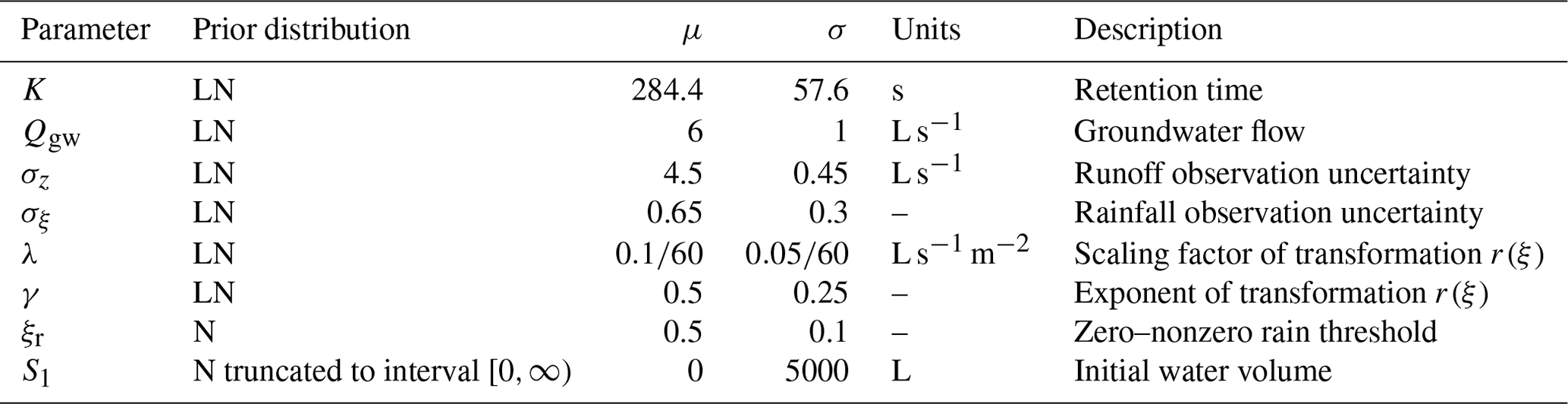
Table 2 Prior probability densities for the inferred parameters, with their mean values (μ), standard deviations (σ) and units. N and LN stand for normal and log-normal distributions, respectively. Note that here, also for log-normal distributions, μ and σ refer to the mean value and standard deviation of a parameter, not its log. The mean and standard deviation for the log, μ_LN and σ_LN, respectively, are given by ${\mathit{\mu }}_{\mathrm{LN}}=\log ({\mathit{\mu }}^{\mathrm{2}}/\sqrt{{\mathit{\mu }}^{\mathrm{2}}+{\mathit{\sigma }}^{\mathrm{2}}})$ and ${\mathit{\sigma }}_{\mathrm{LN}}=\sqrt{\log (\mathrm{1}+{\mathit{\sigma }}^{\mathrm{2}}/{\mathit{\mu }}^{\mathrm{2}})}$.

2.2 The hydrological model

The storm water runoff is modelled by a linear reservoir supplied by rainfall precipitation, P(t), and a constant groundwater flow, Q_gw. The dynamics of the water volume S(t) in the reservoir is thus governed by

$$\begin{array}{}\text{(4)}& \dot{S}\left(t\right)=AP\left(t\right)+Q_{\mathrm{gw}}-Q_{\mathrm{M}}\left(t\right)\mathrm{with}{Q}_{\mathrm{M}}\left(t\right)={\displaystyle \frac{S\left(t\right)}{K}},\end{array}$$

where A is the estimated catchment area contributing to the rainfall-runoff dynamics, Q_M is the hydrological model describing the runoff at the outlet of the system and K is the retention time of the reservoir. It should be noted that the original hydrological model used in Del Giudice et al. (2016) is simplified here by omitting the daily variation due to the wastewater contribution. This is justified by the fact that in the present work we only focus on a single short dataset of 4 h, whereas in Del Giudice et al. (2016) the authors consider three independent datasets covering a time span of about 48 d. One may refer to Sect. 4 for more details.

The discretized form of Eq. (4) reads

$$\begin{array}{}\text{(5)}& S_i=\left(\mathrm{1}-{\displaystyle \frac{\mathrm{d}t}{K}}\right)S_{i-\mathrm{1}}+\left(A{P}_{i-\mathrm{1}}+Q_{\mathrm{gw}}\right)\mathrm{d}t,\end{array}$$

where S_i and P_i are S(t_i) and P(t_i), respectively, with i=1, …, N. It should be noted that explicit methods, such as the forward Euler scheme applied in Eq. (5), are very easy to implement; however, they impose stringent limitations on the time step size to ensure numerical stability. In general, explicit methods might not be sufficiently accurate in regions where the solution exhibits a rapidly varying behaviour. In that case it would be advisable to apply an implicit backward scheme, numerically more stable albeit more difficult to implement. In the application discussed here, we reckon that the problem is simple enough to opt for the explicit forward scheme, thus trading off accuracy for an easier implementation. The intrinsic inaccuracy of the method is attenuated by choosing a discretization time step dt that is sufficiently small compared to the system dynamics timescale.

The predicted discharge $Q_{\mathrm{M},i}(\mathit{\xi },\mathit{\theta })=Q_{\mathrm{M}}\left(t_i\right)$ (i=1, …, N) can be calculated recursively using Eq. (5) with the initial condition Q_M,1(ξ, $\mathit{\theta })=S_{\mathrm{1}}/K$. Straightforward calculations then yield

$$\begin{array}{}\text{(6)}& \begin{array}{rl}{Q}_{\mathrm{M},i}(\mathit{\xi },\mathit{\theta })& ={\displaystyle \frac{S_{\mathrm{1}}}{K}}{\left(\mathrm{1}-{\displaystyle \frac{\mathrm{d}t}{K}}\right)}^{i-\mathrm{1}}+A{\displaystyle \frac{\mathrm{d}t}{K}}{Q}_{\mathrm{M},i}^{\left(\mathit{\xi }\right)}\\ & +\left[\mathrm{1}-{\left(\mathrm{1}-{\displaystyle \frac{\mathrm{d}t}{K}}\right)}^{i-\mathrm{1}}\right]Q_{\mathrm{gw}},\end{array}\end{array}$$

where $Q_{\mathrm{M},i}^{\left(\mathit{\xi }\right)}$ is the ξ-dependent contribution defined recursively as $Q_{\mathrm{M},\mathrm{1}}^{\left(\mathit{\xi }\right)}=\mathrm{0}$ and

$$\begin{array}{}\text{(7)}& Q_{\mathrm{M},i}^{\left(\mathit{\xi }\right)}=\left(\mathrm{1}-{\displaystyle \frac{\mathrm{d}t}{K}}\right)Q_{\mathrm{M},i-\mathrm{1}}^{\left(\mathit{\xi }\right)}+r\left({\mathit{\xi }}_{i-\mathrm{1}}\right)\mathrm{with}i=\mathrm{2},\mathrm{\dots },N,\end{array}$$

where we have used the rainfall potential transformation P_i=r(ξ_i) of Eq. (3). The parameters of the hydrological model, K, Q_gw and the initial water volume S₁, are unknown and to be inferred (see Table 2), while the catchment area is known and fixed as A=11 815.8 m² (Table 1).

2.3 Runoff observation model

The probability distribution for the observed discharges Q_obs given the model predictions $Q_{\mathrm{M},i}(\mathit{\xi },\mathit{\theta })$ is assumed to be a normal error model with standard deviation σ_z, which reads

$$\begin{array}{}\text{(8)}& \begin{array}{rl}f& \left({\mathit{Q}}_{\mathrm{obs}}\mid \mathit{\xi },\mathit{\theta },{\mathit{\sigma }}_z\right)\propto \exp \left[-\left(n_Q+\mathrm{1}\right)\log \left({\mathit{\sigma }}_z\right)\right.\\ & \left.-\sum _{s=\mathrm{1}}^{n_Q+\mathrm{1}}{\displaystyle \frac{{\left(H\left(Q_{\mathrm{obs},\mathrm{s}}\right)-H\left(Q_{\mathrm{M},(s-\mathrm{1})j_Q+\mathrm{1}}(\mathit{\xi },\mathit{\theta })\right)\right)}^{\mathrm{2}}}{\mathrm{2}{\mathit{\sigma }}_z^{\mathrm{2}}}}\right],\end{array}\end{array}$$

where $(s-\mathrm{1})j_Q+\mathrm{1}$, with s=1, …, n_Q+1, are the indices corresponding to real observations in the discretized runoff dimension, and H is a transformation introduced to take the heteroscedasticity of the errors into account (Del Giudice et al., 2016):

$$\begin{array}{}\text{(9)}& H\left(Q\right)=\mathit{\beta }\log \left(\sinh \left({\displaystyle \frac{\mathit{\alpha }+Q}{\mathit{\beta }}}\right)\right),\end{array}$$

with the parameters α=25 L s⁻¹ and β=50 L s⁻¹ (Table 1). Since we are only interested in terms depending on the parameters to be inferred, in Eq. (8) we can neglect constant multiplicative factors such as the Jacobian $\prod _{s=\mathrm{1}}^{n_Q+\mathrm{1}}\frac{\mathrm{d}H}{\mathrm{d}Q}\left(Q_{\mathrm{obs},\mathrm{s}}\right)$.

2.4 Rainfall observation model

The observation error model for the rainfall, given the rainfall potential ξ(t), is defined in the space of the rainfall potential as a normal distribution centred on ξ(t) and with standard deviation σ_ξ. Its discretized form can be expressed in terms of the discretized potential ξ as a product of normal distributions:

$$\begin{array}{}\text{(10)}& f\left({\mathit{\xi }}_{\mathrm{obs}}\mid \mathit{\xi },{\mathit{\sigma }}_{\mathit{\xi }}\right)=\prod _{s=\mathrm{1}}^{n_P+\mathrm{1}}{\mathcal{N}}_{\left({\mathit{\xi }}_{(s-\mathrm{1})j_P+\mathrm{1}},{\mathit{\sigma }}_{\mathit{\xi }}\right)}\left({\mathit{\xi }}_{\mathrm{obs},\mathrm{s}}\right),\end{array}$$

where ξ_obs is defined as the effective rainfall potential generating the observed rainfall, and ${\mathcal{N}}_{(\mathit{\xi },{\mathit{\sigma }}_{\mathit{\xi }})}$ denotes a normal distribution with mean ξ and standard deviation σ_ξ. Note that in Eq. (10) the ${\mathit{\xi }}_{(s-\mathrm{1})j_P+\mathrm{1}}$ values with s=1, …, n_P+1 are the elements of the discretized potential ξ corresponding to time points where rainfall observations are available. This distribution is transformed to real rainfall by the inverse transformation ${\mathit{\xi }}_{\mathrm{obs}}=r^{-\mathrm{1}}\left(P_{\mathrm{obs}}\right)$ (Eq. 3). However, since all ξ values below ξ_r are transformed to zero rain, the transformation r is invertible only where P_obs≠0. Therefore, we need to distinguish two possible regimes, with and without rain:

• At time points where P_obs≠0, the probability density of Eq. (10) reads

  $$\begin{array}{}\text{(11)}& \begin{array}{rl}{f}_{P\ne \mathrm{0}}& \left({\mathit{P}}_{\mathrm{obs}}\mid \mathit{\xi },{\mathit{\sigma }}_{\mathit{\xi }}\right)\propto \exp \left[-n_{P\ne \mathrm{0}}\log \left({\mathit{\sigma }}_{\mathit{\xi }}\right)\right.\\ & \left.-{\displaystyle \frac{\sum _{i,P\ne \mathrm{0}}{\left(r^{-\mathrm{1}}\left(P_{\mathrm{obs},i}\right)-{\mathit{\xi }}_{(i-\mathrm{1})j_P+\mathrm{1}}\right)}^{\mathrm{2}}}{\mathrm{2}{\mathit{\sigma }}_{\mathit{\xi }}^{\mathrm{2}}}}\right]\\ & \times \prod _{i,P\ne \mathrm{0}}{\displaystyle \frac{\mathrm{1}}{{\mathcal{J}}_i}},\end{array}\end{array}$$

  where the sum $\sum _{i,P\ne \mathrm{0}}$ extends only over time points t_i where $P_{\mathrm{obs},i}\ne \mathrm{0}$ and n_P≠0 is the total number of such points. Moreover, the transformation from ξ to P values requires the Jacobians 𝒥_i defined as

  $$\begin{array}{}\text{(12)}& \begin{array}{rl}{\mathcal{J}}_i& ={\displaystyle \frac{\mathrm{d}r}{\mathrm{d}\mathit{\xi }}}\left(r^{-\mathrm{1}}\left(P_{\mathrm{obs},i}\right)\right)=\mathit{\lambda }(\mathrm{1}+\mathit{\gamma }){\left(r^{-\mathrm{1}}\left(P_{\mathrm{obs},i}\right)-{\mathit{\xi }}_{\mathrm{r}}\right)}^{\mathit{\gamma }}\\ & =\mathit{\lambda }(\mathrm{1}+\mathit{\gamma }){\left({\displaystyle \frac{P_{\mathrm{obs},i}}{\mathit{\lambda }}}\right)}^{\frac{\mathit{\gamma }}{\mathrm{1}+\mathit{\gamma }}}.\end{array}\end{array}$$

• At time points where P_obs=0 and therefore ξ_obs can take any value below ξ_r, we integrate the probability density of Eq. (10) over the interval $[-\mathrm{\infty },{\mathit{\xi }}_{\mathrm{r}}]$. This yields the probability of zero observed rain, which turns out to be the cumulative distribution function of the normal distribution; that is,

  $$\begin{array}{}\text{(13)}& \begin{array}{rl}{f}_{P=\mathrm{0}}& \left({\mathit{P}}_{\mathrm{obs}}\mid \mathit{\xi },{\mathit{\sigma }}_{\mathit{\xi }}\right)\\ & =\prod _{i,P=\mathrm{0}}{\displaystyle \frac{\mathrm{1}}{\mathrm{2}}}\left[\mathrm{1}+\mathrm{erf}\left({\displaystyle \frac{{\mathit{\xi }}_{\mathrm{r}}-{\mathit{\xi }}_{(i-\mathrm{1})j_P+\mathrm{1}}}{{\mathit{\sigma }}_{\mathit{\xi }}\sqrt{\mathrm{2}}}}\right)\right],\end{array}\end{array}$$

  where the product $\prod _{i,P=\mathrm{0}}$ extends over time points t_i where $P_{\mathrm{obs},i}=\mathrm{0}$.

Therefore,

$$f\left({\mathit{P}}_{\mathrm{obs}}\mid \mathit{\xi },{\mathit{\sigma }}_{\mathit{\xi }}\right)=f_{P\ne \mathrm{0}}\left({\mathit{P}}_{\mathrm{obs}}\mid \mathit{\xi },{\mathit{\sigma }}_{\mathit{\xi }}\right)f_{P=\mathrm{0}}\left({\mathit{P}}_{\mathrm{obs}}\mid \mathit{\xi },{\mathit{\sigma }}_{\mathit{\xi }}\right).$$

2.5 The priors

At this point, the only elements of Eq. (1) that still need to be defined are the prior distributions f(θ, σ_ξ, σ_z) and f(ξ). The former is simply the product of normal or log-normal univariate probability densities for each individual parameter to be inferred. The parameter vector θ here includes the parameters of the hydrological model, K, Q_gw and S₁, as well as those of the transformation r (Eq. 3), that is, ξ_r, λ and γ. We infer a total of eight parameters, listed in Table 2. For the parameters S₁ and ξ_r the prior densities are assumed to be normal distributions, whereas for the other parameters (K, Q_gw, λ and γ) the prior densities are assumed to be log-normal distributions:

$$\begin{array}{}\text{(14)}& f\left(\mathit{\theta }\right)\propto \exp \left[-\log \mathit{\theta }-{\displaystyle \frac{{\left(\log \mathit{\theta }-{\mathit{\mu }}_{\mathrm{LN}}\right)}^{\mathrm{2}}}{\mathrm{2}{\mathit{\sigma }}_{\mathrm{LN}}^{\mathrm{2}}}}\right],\end{array}$$

with the mean and standard deviation μ_LN and σ_LN, respectively. Analogous log-normal distributions are assumed for the rainfall and discharge observation uncertainties, σ_ξ and σ_z, respectively. The prior distributions for all parameters to be inferred, with their mean values and standard deviations, are summarized in Table 2.

Our prior knowledge of the rainfall potential ξ is defined in terms of a function 𝒮(ξ), called action (Lau and Lubensky, 2007; Albert et al., 2016), as

$$\begin{array}{}\text{(15)}& f\left(\mathit{\xi }\right)\propto \exp \left[-\mathcal{S}\left(\mathit{\xi }\right)-{\mathit{\xi }}_{\mathrm{1}}^{\mathrm{2}}/\mathrm{2}\right],\end{array}$$

where the action can be written in its discretized form for the SDE model of Eq. (2) as (see Sect. S1 in the Supplement)

$$\begin{array}{}\text{(16)}& \mathcal{S}\left(\mathit{\xi }\right)\approx {\displaystyle \frac{{\mathit{\xi }}_N^{\mathrm{2}}}{\mathrm{4}}}-{\displaystyle \frac{{\mathit{\xi }}_{\mathrm{1}}^{\mathrm{2}}}{\mathrm{4}}}+\sum _{i=\mathrm{2}}^N\left[{\displaystyle \frac{\mathit{\tau }}{\mathrm{4}\mathrm{d}t}}{\left({\mathit{\xi }}_i-{\mathit{\xi }}_{i-\mathrm{1}}\right)}^{\mathrm{2}}+{\displaystyle \frac{\mathrm{d}t}{\mathrm{4}\mathit{\tau }}}{\mathit{\xi }}_i^{\mathrm{2}}\right],\end{array}$$

and the initial condition for ξ is specified as the marginal distribution of a standard OU process, which is a standard normal distribution for ξ₁. It is noteworthy that the HMC method described here always requires an explicit analytical form for the action 𝒮(ξ), which is essentially just the negative log of the prior density f(ξ), which is also needed in any other Metropolis-type sampling algorithm. Although in this study we follow the approach of Del Giudice et al. (2016) and resort to a linear OU process as a precipitation generator, an analytical expression for the action is generally readily available, even for more complex and nonlinear SDE models. More details about the procedure to derive the action for generic SDE models can be found in the Supplement (Sect. S1).

Before setting off to implement the HMC algorithm, we take one further convenient step; i.e. we apply the transformation from the coordinates ξ to the so-called staging variables u (Tuckerman et al., 1993) using

$$\begin{array}{}\text{(17)}& u_{s{j}_P+\mathrm{1}}={\mathit{\xi }}_{s{j}_P+\mathrm{1}}\mathrm{with}s=\mathrm{0},\mathrm{\dots },n_P,\end{array}$$

which leaves the components corresponding to measurement points unchanged, and

$$\begin{array}{}\text{(18)}& \begin{array}{rl}{u}_{s{j}_P+k}=& {\mathit{\xi }}_{s{j}_P+k}-{\mathit{\xi }}_{s{j}_P+k}^{*}\mathrm{with}s=\mathrm{0},\mathrm{\dots },n_P-\mathrm{1}\\ & \mathrm{and}k=\mathrm{2},\mathrm{\dots },j_P\end{array}\end{array}$$

and with

$$\begin{array}{}\text{(19)}& {\mathit{\xi }}_{s{j}_P+k}^{*}={\displaystyle \frac{\left(k\mathrm{-}\mathrm{1}\right){\mathit{\xi }}_{s{j}_P+k+\mathrm{1}}+{\mathit{\xi }}_{s{j}_P+\mathrm{1}}}{k}}\end{array}$$

for the intermediate discretization points. Also relevant are the inverse transformations for the discretization points,

$$\begin{array}{}\text{(20)}& \begin{array}{rl}{\mathit{\xi }}_{s{j}_P+k}=& \sum _{l=k}^{j_P+\mathrm{1}}{\displaystyle \frac{k-\mathrm{1}}{l-\mathrm{1}}}{u}_{s{j}_P+l}+{\displaystyle \frac{j_P-k+\mathrm{1}}{j_P}}{u}_{s{j}_p+\mathrm{1}},\\ & \mathrm{with}s=\mathrm{0},\mathrm{\dots },n_P-\mathrm{1}\mathrm{and}k=\mathrm{2},\mathrm{\dots },j_P.\end{array}\end{array}$$

The action 𝒮(ξ) (Eq. 16) can be formulated in the space of u coordinates (see Sect. S2) as

$$\begin{array}{}\text{(21)}& \begin{array}{rl}\mathcal{S}\left(\mathit{u}\right)& ={\displaystyle \frac{k\mathit{\tau }}{\mathrm{4}(k-\mathrm{1})\mathrm{d}t}}\sum _{s=\mathrm{1}}^{n_P}\sum _{k=\mathrm{2}}^{j_P}{u}_{(s-\mathrm{1})j_P+k}^{\mathrm{2}}\\ & +{\displaystyle \frac{\mathit{\tau }}{\mathrm{4}{j}_P\mathrm{d}t}}\sum _{s=\mathrm{1}}^{n_P}{\left(u_{(s-\mathrm{1})j_P+\mathrm{1}}-u_{s{j}_P+\mathrm{1}}\right)}^{\mathrm{2}}\\ & +{\displaystyle \frac{u_N^{\mathrm{2}}}{\mathrm{4}}}-{\displaystyle \frac{u_{\mathrm{1}}^{\mathrm{2}}}{\mathrm{4}}}+{\displaystyle \frac{\mathrm{d}t}{\mathrm{4}\mathit{\tau }}}\sum _{s=\mathrm{1}}^{n_P}\left[u_{s{j}_P+\mathrm{1}}^{\mathrm{2}}\right.\\ & +\sum _{k=\mathrm{2}}^{j_P}\left(\sum _{l=k}^{j_P+\mathrm{1}}{\displaystyle \frac{k-\mathrm{1}}{l-\mathrm{1}}}{u}_{(s-\mathrm{1})j_P+l}\right.\\ & \left.{\left.+{\displaystyle \frac{j_P-k+\mathrm{1}}{j_P}}{u}_{(s-\mathrm{1})j_P+\mathrm{1}}\right)}^{\mathrm{2}}\right],\end{array}\end{array}$$

while the initial condition ${\mathit{\xi }}_{\mathrm{1}}^{\mathrm{2}}/\mathrm{2}$ can be simply replaced by $u_{\mathrm{1}}^{\mathrm{2}}/\mathrm{2}$. This coordinate transformation, analogous to a transformation to canonical coordinates, is not a strict requirement of the HMC method and undoubtedly adds a further degree of complexity to the overall strategy. However, it also bears remarkable computational benefits. Indeed, the first term on the right-hand side of Eq. (21) describes the potential of a system of uncoupled harmonic oscillators, which can be effortlessly solved analytically. These dynamics also turn out to be much faster than all other characteristic timescales of the system. In Sect. 3 we will describe in detail how this can be exploited.

3 The HMC algorithm

The HMC algorithm interprets the negative logarithm of the posterior density as a potential energy driving the dynamics of a fictitious statistical mechanics system whose configurations, namely, the system's degrees of freedom, are described by combinations of both parameters (θ, σ_ξ, σ_z) and realizations ξ of the stochastic process ξ(t). The degrees of freedom of the system are coupled to conjugate variables, that is, to momenta π, paired with the parameters (θ, σ_ξ, σ_z), and p, paired with the realizations ξ. The posterior density of Eq. (1) can be rewritten in the following discretized form:

$$\begin{array}{}\text{(22)}& \begin{array}{rl}f& \left(\mathit{\xi },\mathit{\theta },{\mathit{\sigma }}_{\mathit{\xi }},{\mathit{\sigma }}_z\mid {\mathit{P}}_{\mathrm{obs}},{\mathit{Q}}_{\mathrm{obs}}\right)\propto \int \exp \\ & \left[-{\mathcal{H}}_{\mathrm{HMC}}\left(\mathit{\xi },\mathit{\theta },{\mathit{\sigma }}_{\mathit{\xi }},{\mathit{\sigma }}_z;\mathit{\pi },\mathit{p}\right)\right]\mathrm{d}\mathit{\pi }\mathrm{d}\mathit{p},\end{array}\end{array}$$

with the Hamiltonian ℋ_HMC defined as

$$\begin{array}{}\text{(23)}& \begin{array}{rl}{\mathcal{H}}_{\mathrm{HMC}}& \left(\mathit{\xi },\mathit{\theta },{\mathit{\sigma }}_{\mathit{\xi }},{\mathit{\sigma }}_z;\mathit{\pi },\mathit{p}\right)=-\log \left[f\left(\mathit{\xi },\mathit{\theta },{\mathit{\sigma }}_{\mathit{\xi }},{\mathit{\sigma }}_z\mid \right.\right.\\ & \left.\left.{\mathit{P}}_{\mathrm{obs}},{\mathit{Q}}_{\mathrm{obs}}\right)\right]+\sum _{\mathit{\alpha }=\mathrm{1}}^{N_{\mathrm{p}}}{\displaystyle \frac{{\mathit{\pi }}_{\mathit{\alpha }}^{\mathrm{2}}}{\mathrm{2}{m}_{\mathit{\alpha }}}}+\sum _{i=\mathrm{1}}^N{\displaystyle \frac{p_i^{\mathrm{2}}}{\mathrm{2}{m}_i}},\end{array}\end{array}$$

where N_p is the number of parameters to be inferred (eight in our case). We have introduced two auxiliary terms on the right-hand side using the vectors of momenta π and p, akin to the kinetic energies associated with the degrees of freedom of the fictitious statistical mechanics system.

The masses m_α and m_i are tuning parameters of the algorithm. Since we want the coordinates ξ_i corresponding to actual observations to be more tightly constrained than those corresponding to the intermediate discretization points, we set $m_{s{j}_P+\mathrm{1}}=M$ with s=0, …, n_P, for the “heavy” measurement points, and $m_{s{j}_P+k}=m$ with s=0, …, n_P−1 and k=2, …, j_P, for the “lighter” intermediate discretization points, with M≫m.

The potential energy, proportional to −log [f(ξ, θ, σ_ξ, σ_z∣P_obs, Q_obs)], guarantees that each state of the system is compatible with the observations and constrained within their measurement uncertainties, as well as with the prior distributions for both model parameters and rainfall potential realizations ξ.

The HMC algorithm iterates the following steps. First, vectors of momenta π and p are drawn from the zero-mean normal distributions defined by the kinetic terms in Eq. (23). Then, the system is left to evolve for a fictitious time interval dτ in the (ξ, θ, σ_ξ, σ_z; π, p) phase space according to Hamilton's equations. This Hamiltonian dynamics is controlled by tuning the fictitious masses in Eq. (23), which represent the variances of the normal distributions for the corresponding momenta. Finally, the discretization error on the energy conservation introduced with the integration of Hamilton's equations is corrected by a Metropolis accept/reject step. The resulting marginal distributions of the Markov chains of the system configurations (ξ, θ, σ_ξ, σ_z) represent a sample of the sought posterior density. The method is described in detail in Albert et al. (2016).

Note that the presence of pronounced local minima in a high-dimensional phase space might represent an insurmountable obstacle, even for more refined implementations of the HMC method, for example, with automatic tuning of the algorithm hyper-parameters (see Sect. 4.1 for more details). In that case one would have to resort to further enhancements such as metadynamics (Laio and Gervasio, 2008) or parallel tempering (Swendsen and Wang, 1986; Marinari and Parisi, 1992; Earl and Deem, 2005). However, this is not an issue in the specific application discussed here.

Using Eq. (1) and the definitions given in Sect. 2.1–2.5, we write the HMC Hamiltonian as

$$\begin{array}{}\text{(24)}& {\mathcal{H}}_{\mathrm{HMC}}={\mathcal{H}}_N+{\mathcal{H}}_n+{\mathcal{H}}_{\mathrm{1}},\end{array}$$

where the three components describe dynamics occurring on different timescales. Let us consider them individually. The first component,

$$\begin{array}{}\text{(25)}& {\mathcal{H}}_N=\sum _{s=\mathrm{1}}^{n_P}\sum _{k=\mathrm{2}}^{j_P}\left[{\displaystyle \frac{p_{(s-\mathrm{1})j_P+k}^{\mathrm{2}}}{\mathrm{2}m}}+{\displaystyle \frac{k\mathit{\tau }}{\mathrm{4}(k-\mathrm{1})\mathrm{d}t}}{u}_{(s-\mathrm{1})j_P+k}^{\mathrm{2}}\right],\end{array}$$

contains the harmonic term for the intermediate discretization points from the action of Eq. (21) and scales as the total number of discretization points N. The second component,

$$\begin{array}{}\text{(26)}& \begin{array}{rl}{\mathcal{H}}_n& =\sum _{s=\mathrm{1}}^{n_P+\mathrm{1}}{\displaystyle \frac{p_{(s-\mathrm{1})j_P+\mathrm{1}}^{\mathrm{2}}}{\mathrm{2}M}}+\sum _{s=\mathrm{1}}^{n_P}{\displaystyle \frac{\mathit{\tau }}{\mathrm{4}{j}_P\mathrm{d}t}}{\left(u_{(s-\mathrm{1})j_P+\mathrm{1}}-u_{s{j}_P+\mathrm{1}}\right)}^{\mathrm{2}}\\ & +\sum _{s=\mathrm{1}}^{n_Q+\mathrm{1}}{\displaystyle \frac{{\left(H\left(Q_{\mathrm{obs},\mathrm{s}}\right)-H\left(Q_{\mathrm{M},(s-\mathrm{1})j_Q+\mathrm{1}}(\mathit{u},\mathit{\theta })\right)\right)}^{\mathrm{2}}}{\mathrm{2}{\mathit{\sigma }}_z^{\mathrm{2}}}}\\ & +\left(n_Q+\mathrm{1}\right)\log \left({\mathit{\sigma }}_z\right)+\sum _{i,P\ne \mathrm{0}}\left[{\displaystyle \frac{{\left(r^{-\mathrm{1}}\left(P_{\mathrm{obs},i}\right)-u_{(i-\mathrm{1})j_P+\mathrm{1}}\right)}^{\mathrm{2}}}{\mathrm{2}{\mathit{\sigma }}_{\mathit{\xi }}^{\mathrm{2}}}}\right.\\ & \left.+\log {\mathcal{J}}_i\right]+n_{P\ne \mathrm{0}}\log \left({\mathit{\sigma }}_{\mathit{\xi }}\right)-\sum _{i,P=\mathrm{0}}\log \\ & \left[{\displaystyle \frac{\mathrm{1}}{\mathrm{2}}}\left(\mathrm{1}+\mathrm{erf}\left({\displaystyle \frac{{\mathit{\xi }}_{\mathrm{r}}-u_{(i-\mathrm{1})j_P+\mathrm{1}}}{{\mathit{\sigma }}_{\mathit{\xi }}\sqrt{\mathrm{2}}}}\right)\right)\right],\end{array}\end{array}$$

contains a harmonic term for the measurement points from Eq. (21) and the observation error models f(Q_obs∣u, θ, σ_z) and f(P_obs∣u, σ_ξ) from Sect. 2.3 and 2.4, respectively. All the components of Eq. (26) scale as the number of observations n_P or n_Q. Note that both the observation models for runoff and rainfall are rewritten in the space of u-coordinates. While the coordinate transformation ξ→u is straightforward for the rainfall observation model, which only depends on measurement points, it is somewhat more cumbersome for the runoff observation model, which requires the ξ-dependent component $Q_{\mathrm{M},i}^{\left(\mathit{\xi }\right)}$ (see Eqs. 6 and 7) to be rewritten in the u space as $Q_{\mathrm{M},i}^{\left(u\right)}$. Such transformation is described in Sect. S3. The third component of the Hamiltonian ℋ_HMC is

$$\begin{array}{}\text{(27)}& \begin{array}{rl}{\mathcal{H}}_{\mathrm{1}}& =\sum _{\mathit{\alpha }=\mathrm{1}}^{N_{\mathrm{p}}}{\displaystyle \frac{{\mathit{\pi }}_{\mathit{\alpha }}^{\mathrm{2}}}{\mathrm{2}{m}_{\mathit{\alpha }}}}+{\displaystyle \frac{u_N^{\mathrm{2}}}{\mathrm{4}}}+{\displaystyle \frac{u_{\mathrm{1}}^{\mathrm{2}}}{\mathrm{4}}}+{\displaystyle \frac{\mathrm{d}t}{\mathrm{4}\mathit{\tau }}}\sum _{s=\mathrm{1}}^{n_P}\left[u_{s{j}_P+\mathrm{1}}^{\mathrm{2}}\right.\\ & +\sum _{k=\mathrm{2}}^{j_P}\left(\sum _{l=k}^{j_P+\mathrm{1}}{\displaystyle \frac{k-\mathrm{1}}{l-\mathrm{1}}}{u}_{(s-\mathrm{1})j_P+l}\right.\\ & \left.{\left.+{\displaystyle \frac{j_P-k+\mathrm{1}}{j_P}}{u}_{(s-\mathrm{1})j_P+\mathrm{1}}\right)}^{\mathrm{2}}\right]+\sum _{\mathit{\theta }\in {\mathit{\theta }}_{\mathrm{N}}}{\displaystyle \frac{{\left(\mathit{\theta }-{\mathit{\mu }}_{\mathit{\theta }}\right)}^{\mathrm{2}}}{\mathrm{2}{\mathit{\sigma }}_{\mathit{\theta }}^{\mathrm{2}}}}\\ & +\sum _{\mathit{\theta }\in {\mathit{\theta }}_{\mathrm{LN}}}\left[\log \mathit{\theta }+{\displaystyle \frac{{\left(\log \mathit{\theta }-{\mathit{\mu }}_{\mathrm{LN},\mathit{\theta }}\right)}^{\mathrm{2}}}{\mathrm{2}{\mathit{\sigma }}_{\mathrm{LN},\mathit{\theta }}^{\mathrm{2}}}}\right],\end{array}\end{array}$$

which includes the remaining terms from the rainfall potential prior (Eq. 15) and the model parameter priors. The latter, i.e. the last two terms in Eq. (27), are sums over the parameters θ_N=(S₁, ξ_r) and ${\mathit{\theta }}_{\mathrm{LN}}=(K,Q_{\mathrm{gw}},\mathit{\lambda },\mathit{\gamma },{\mathit{\sigma }}_{\mathit{\xi }},{\mathit{\sigma }}_z)$, whose prior densities are normal and log-normal distributions, respectively. Note the sign change in front of the term $u_{\mathrm{1}}^{\mathrm{2}}/\mathrm{4}$ with respect to Eq. (21) due to the initial condition for u₁ (see Eq. 15). The component ℋ₁ does not grow unbounded with either N or n_P or n_Q (notice that $\mathrm{d}t\propto \mathrm{1}/N$).

Let us now exploit the different timescales characterizing the three components of the Hamiltonian ℋ_HMC. We assume the regime ${\mathcal{H}}_N\gg {\mathcal{H}}_n\approx {\mathcal{H}}_{\mathrm{1}}$, implying that the number of data points is not too large and that the total number of discretization points is instead large compared to the number of data points. Under these conditions, the dynamics of the system occur on very different timescales. In particular, the dynamics described by ℋ_N are much faster than the other components of the Hamiltonian and therefore impose the most stringent limitations on the step size for the numerical integration of Hamilton equations. However, we use Trotter's formula (Tuckerman et al., 1992) to construct a reversible molecular dynamics integrator to take the different timescales into account as described in Albert et al. (2016). In particular, we exploit the fact that the much faster dynamics of the intermediate discretization points described by ℋ_N is analogous to a system of uncoupled harmonic oscillators that can be solved analytically. This analytical solution gives a significant boosting contribution to the intrinsic efficiency of the HMC algorithm. The “slow” remaining components of the Hamiltonian, ℋ_n and ℋ₁, can be integrated using a much larger integration step, which allows us to explore the high-dimensional parameter space of the system with remarkable efficiency.

As explained in Albert et al. (2016), the decoupling of the different dynamics and the analytical solution of the expensive fast component is always possible for one-dimensional SDE models. It is also possible in the case of multiple independent variables, where the decoupling procedure can be applied to each of them individually. In this way, our HMC approach covers a significant range of possible hydrological modelling scenarios. However, in this work we focus only on 1D models, leaving the exploration of higher-dimensional models to future studies.

4 Case study

In this work we apply a HMC method with a stochastic input model (SIP) following Del Giudice et al. (2016) to investigate the rainfall-runoff dynamics of an urban catchment based on real rainfall and runoff observations. The catchment is a small and fast-reacting sewer network in Adliswil, near Zurich, Switzerland. Two typical scenarios of possible rainfall data are considered here; that is, we use the following: (1) high-resolution data, with a time resolution of 1 min, recorded by two pluviometers (denoted P1_a and P1_b) located in the immediate vicinity of the catchment area, and (2) low-resolution data, with a time resolution of 10 min, recorded by a pluviometer (denoted P2) located further away from the catchment, at a distance of about 6 km. We shall refer to the two scenarios as scenario 1 (Sc1) and scenario 2 (Sc2), respectively. More information can be found in Del Giudice et al. (2016).

The precipitation data P_obs used in this study contain $n_P+\mathrm{1}=\mathrm{241}$ observations in Sc1 and $n_P+\mathrm{1}=\mathrm{25}$ observations in Sc2, covering a total observation time T=240 min. The initial and final observation time points are the same for both scenarios and include a storm event that took place in the evening of 10 June 2013, approximately between 18:00 and 20:00 LT. We should mention here a substantial difference with respect to Del Giudice et al. (2016). In their work, the authors base the inference process on three independent time series covering a total observation time of 1710 min distributed over a time span of 48 d. In the work presented here, instead, we consider only the first of the three time series, which also happens to be the shortest. Although the HMC algorithm could deal with the multiple independent time series used by Del Giudice et al. (2016), our simplification finds its justification in that it reduces the computational requirements of the problem, without compromising the goal of our work, that is, showing the feasibility of Bayesian inference of both model parameters and high-dimensional system states (i.e. the ξ's) under the considerable hardship of a stochastic input process.

The discharge flow at the outlet of the catchment was measured with a time resolution of 4 min, and the output observations Q_obs, containing $n_Q+\mathrm{1}=\mathrm{61}$ measurements, are the same for both scenarios and considered accurate compared to the precipitation data. The initial and final observation times are the same as for the input time series. The time series for the observed outputs (Q_obs) as well as the observed precipitation (P_obs) for both Sc1 and Sc2 are shown in Fig. 5.

Scenario 1 represents a best-case scenario of input data availability, and we shall therefore classify it as the accurate input scenario, while scenario 2 is a typical example of inaccurate and unreliable input data due to both its sparsity and the distance of the P2 rain gauge from the area of interest. The runoff observations Q_obs exhibit an important rainfall event (the storm) represented by an evident discharge peak. While this event is properly recorded by the rain gauges of Sc1, the inaccurate input data of Sc2 misleadingly recorded the event at an earlier time period, presumably when the storm passed over the location of the distant pluviometer P2.

We are particularly interested in the performance of the combined SIP-HMC method in the latter case, characterized by faulty precipitation data, which clearly represents the most challenging scenario and therefore the hardest test for the HMC method. Therefore, our work consists of three main steps. First, we use the combined SIP-HMC approach described above, with the inaccurate precipitation data P_obs of Sc2, to calibrate the model and infer the unknown “true” average rainfall pattern over the catchment. Then, we use the accurate rainfall observations from Sc1 as a reference to assess the quality of the simulated “true” rain. Finally, we repeat the calibration process using the accurate data of Sc1 as a further validation for the method.

4.1 Implementation

The HMC algorithm is implemented in C$++$14 using the open-source ADEPT library (Automatic Differentiation using Expression Templates, version 1.1) for the calculation of the gradients of the Hamiltonian ℋ_HMC (Hogan, 2014). Automated differentiation allows us to automatize the algorithm to a large extent, thus making it applicable to a broad range of models with relatively little implementation effort. Indeed, for the hydrological application presented here we resorted to the algorithm already implemented for the simpler toy model studied in Albert et al. (2016). The implementation of the algorithm remained essentially unaltered, except only for the Hamiltonian ℋ_HMC that had to be modified according to Eqs. (25)–(27).

The simulations were run on 2.6–3.7 GHz processors Xeon-Gold 6142 with 196 GB of memory. We observed a relatively short burn-in phase for all inferred parameters, suggesting the possibility of a straightforward (embarrassingly simple) parallelization of the algorithm obtained by simply breaking up the Markov chains into smaller independent chains that can then be executed as parallel processes. It is well known that Markov Chain Monte Carlo (MCMC) methods, like the HMC algorithm employed here, are indeed very well suited for parallel computing. This kind of approach was proven successful in Albert et al. (2016) with a toy system. In that case we used an OpenMP-based parallel implementation of the algorithm and observed a reasonably linear strong scaling behaviour with up to 16 parallel processes.

In the present work, for Sc2, after an initial single burn-in chain of 75 000 steps, which is then disregarded, we limited ourselves to running four independent Markov chains each of length 100 000 steps based on a serial implementation of the algorithm. For Sc1, which is faster than Sc2 due to the much smaller number of intermediate discretization points (see below for more details), we considered a single chain of 750 000 steps and disregarded the first 150 000 steps. The extension of the current serial version to an OpenMP parallel implementation of the HMC code would be straightforward.

We set a fine-grid time step dt=10 s and a total number of discretization points N=1441 for both scenarios. It is easy to verify that these conditions are fulfilled by setting the number of bins between consecutive observations to j_P=6 or j_P=60 on the precipitation dimension for Sc1 and Sc2, respectively, and j_Q=24 for the runoff dimension. The initial configuration of the system state ξ for the burn-in chain is a random realization of the OU process of Eq. (2), while the parameters are set equal to the mean values of their prior distributions (see Table 2).

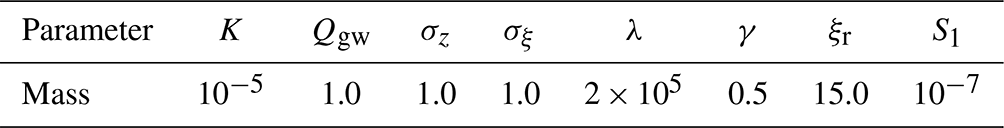
The algorithm requires tuning of two sets of parameters, that is, the parameters defining the Hamiltonian propagator in the molecular dynamics part of the HMC algorithm (see Eq. 26 in Albert et al., 2016) and the masses m, M and m_α defining the kinetic energy of the system in ℋ_HMC. Thus, in the Hamiltonian propagator we set the integration time Δτ=0.015 and the number of integration steps P=3, while the masses were set to m=0.4 for the intermediate discretization points and M=1.6 for the measurement points. The masses for the inferred parameters are given in Table 3.

It should be noted that the integration time interval of the Hamiltonian propagator could be automatically optimized by employing the so-called No-U-Turn Sampler (NUTS) (Hoffman and Gelman, 2014), and the masses of the kinetic terms could be tuned by adapting their values to the curvature of the energy landscape (Girolami and Calderhead, 2011; Hartmann et al., 2022). The efficiency of the HMC algorithm would surely benefit from these approaches but at some cost in terms of implementation efforts. In this work we simply opt for a manual tuning of the hyper-parameters mentioned above.

In Sc2, a full Markov chain of 100 000 steps requires approximately 1 h and 20 min on our hardware, while a chain of 750 000 in Sc1 requires about 2.5 h. At each iteration of the chain, the algorithm infers 1449 parameters, that is, eight model parameters (θ, σ_ξ, σ_z) and N=1441 coordinates of the system state ξ.

The algorithm spends ≈96 % of the total run time in the molecular dynamics part, that is, in the loop for the integration of Hamilton's equations. The loop is called once in each step of the Markov chain. At each call, the HMC algorithm performs one evaluation of the posterior function ℋ_HMC, for the calculation of the system energy, and six evaluations of its derivatives (with P=3 integration steps). In our case study and implementation of the algorithm, each differentiation of the posterior function turns out to be about 6 times more expensive than its plain evaluation. Although this factor is only indicative and may vary to some extent between different implementations, the calculation of the derivatives in general represents the major bottleneck in the performance of the HMC algorithm.

Table 3 Parameter masses m_α for the kinetic term of Eq. (27).

4.2 Results

The Markov chains for the model parameters generated using the unreliable input data of Sc2 are shown in Fig. 1. A simple visual inspection leads us to conclude with a good confidence that the chains have appropriately converged, and the mixing in parameters space is satisfactory. Figure 2 shows the Markov chains for the same model parameters, generated using the accurate rainfall observations of Sc1. The corresponding marginal posterior probability densities for the model parameters, for both Sc2 and Sc1, are shown in Fig. 3 together with the initial prior distributions.

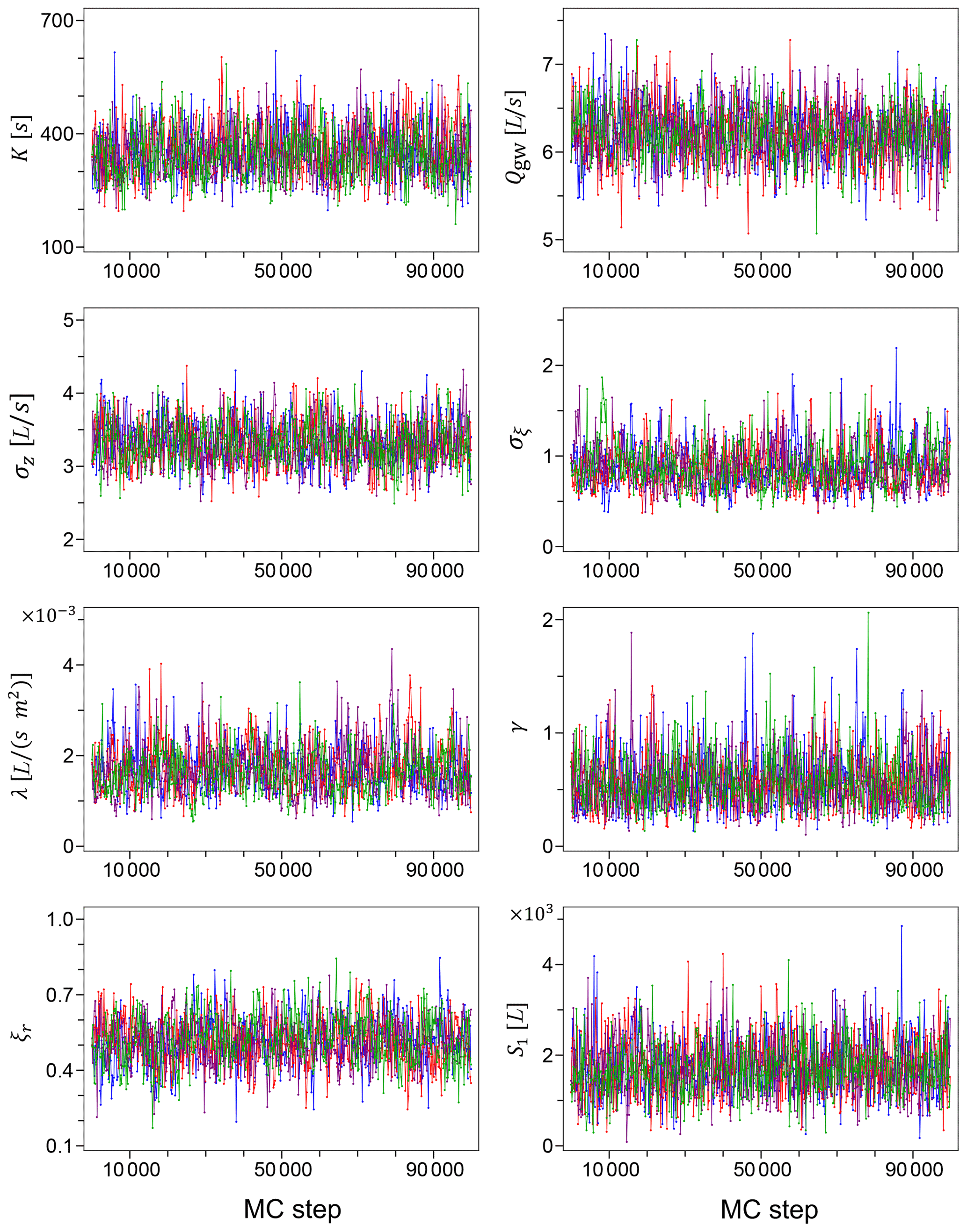
Figure 1 Markov chains for the model parameters generated using the faulty input data of Sc2. As explained in Sect. 4.1, we have four independent chains for each parameter.

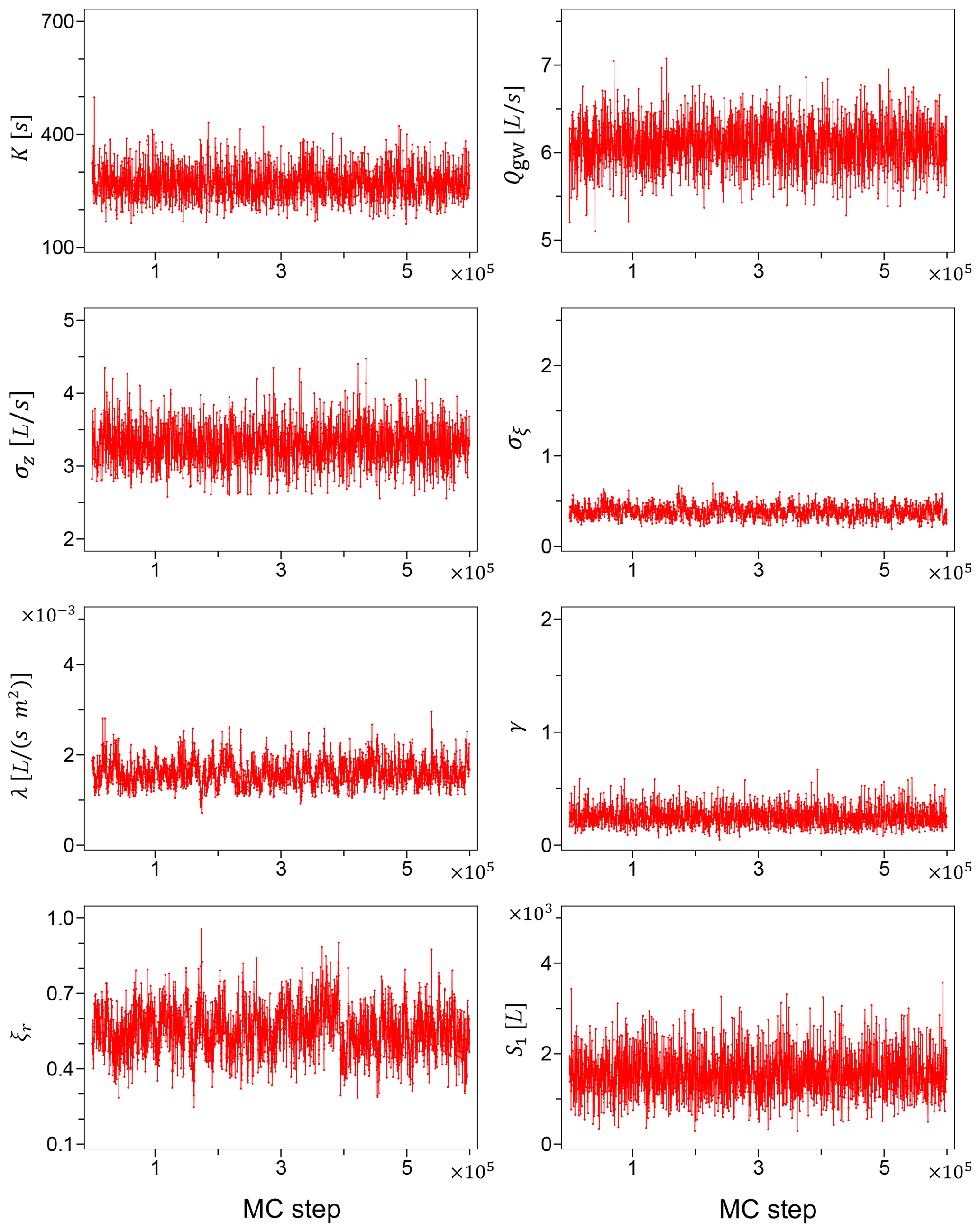
Figure 2 Markov chains for the model parameters from Sc1. Unlike Sc2, we have a single chain for each parameter in this case.

The two scenarios bear some interesting albeit not surprising differences. In general, the posterior distributions generated in Sc1 tend to be narrower than the corresponding distributions in Sc2, clearly reflecting the accuracy of the precipitation data. The rainfall observational error σ_ξ appears to be also strongly shifted to lower values in Sc1, indicative of the reduced uncertainty compared to the faulty Sc2. On the other hand, the practically identical posterior densities for the runoff observational error σ_z reflect the fact that the discharge data Q_obs are the same for both scenarios.

Moreover, Fig. 3 shows that among the rain-related parameters of the transformation of Eq. (3), the marginal posterior for the exponent γ exhibits the largest shift towards smaller values when going from Sc2 to Sc1, while the zero–nonzero rain threshold ξ_r is only mildly shifted to larger values, and the scaling factor λ seems to be essentially unaltered, besides the narrowing effect due to the improved accuracy of the precipitation data. The algorithm automatically tunes the parameters of the rainfall potential transformation to match the available rainfall data. The smaller value of the exponent γ in Sc1 compared to Sc2 reflects this attempt of the algorithm to find a better fit to the rain observations, especially where precipitation values are large.

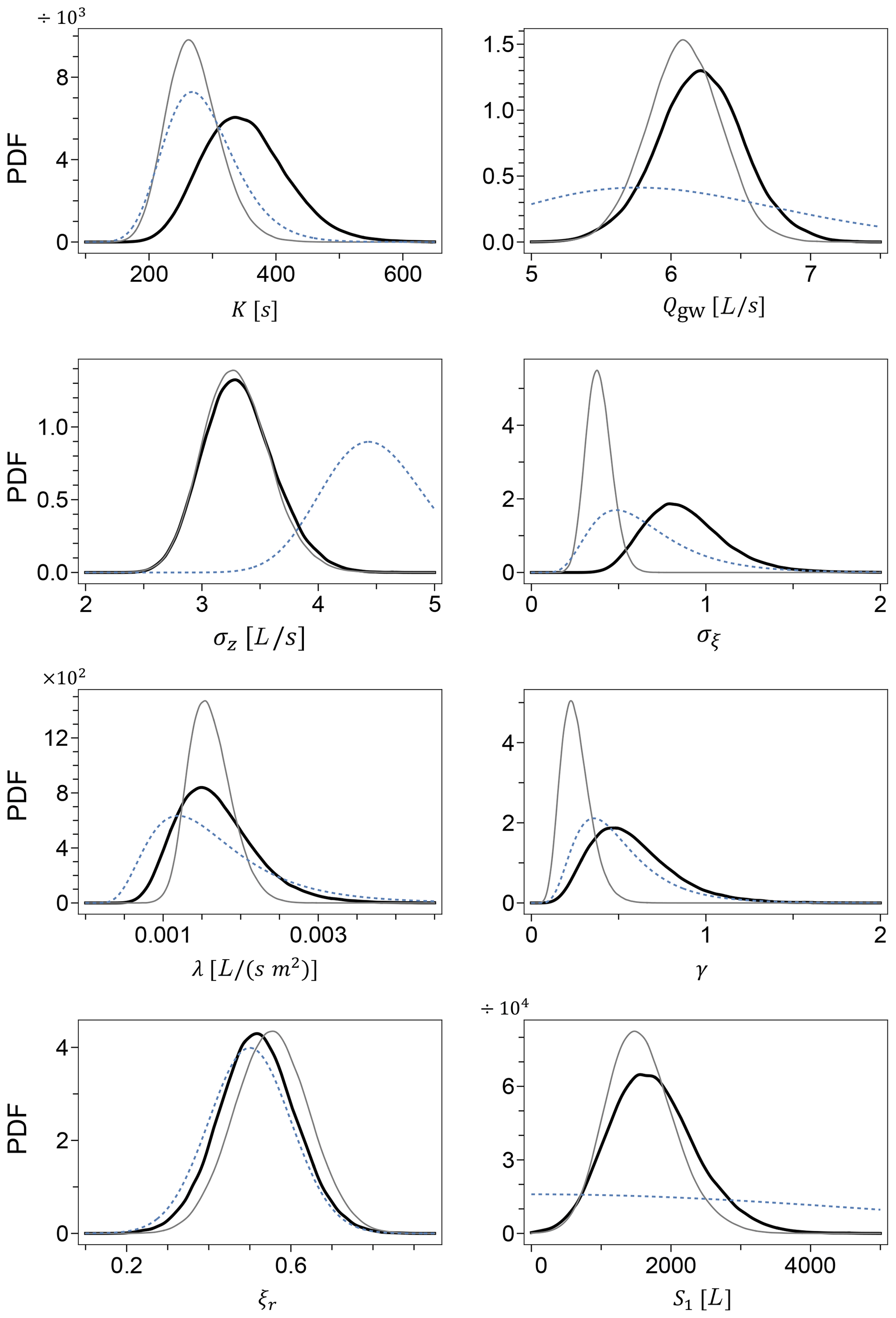
Figure 3 Marginal posterior probability densities for the model parameters from Sc2 (thick black line) and Sc1 (thin grey line). The dashed lines represent the prior densities.

Among the parameters of the hydrological model, the marginal distribution of the retention time K appears to be clearly shifted to smaller values in Sc1, suggesting a faster reacting system compared to Sc2, while the groundwater contributions Q_gw and the initial water volume S₁ exhibit only very minor shifts.

In Fig. 4 we also show two typical Markov chains from Sc2 for the stochastic process ξ, evaluated at two time points with and without rain. The two chains clearly fluctuate above (point with rain) and below (point without rain) the inferred zero–nonzero rain threshold ξ_r. Analogously to the model parameters, the Markov chains for ξ appear to have converged and to be well mixed. The ξ chains in Sc1 are qualitatively identical to those of Sc2 and are not shown here.

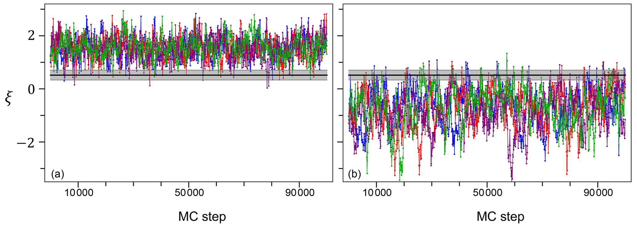
Figure 4 Typical Markov chains for two different points of the stochastic process ξ from Sc2, with (a) and without (b) rain. The horizontal solid line is the median of the inferred zero–nonzero rain threshold ξ_r, while the shaded area represents its uncertainty given by the 2.5 and 97.5 percentiles. As in Fig. 1, we have four independent chains for each point.

In the left panels of Fig. 5 we compare the inferred discharge and rainfall patterns, Q_M(ξ,θ) and r(ξ), respectively, based on the inaccurate rainfall data of Sc2, with the observed runoff Q_obs and precipitation P_obs. The measured outflow (upper panel, open red squares) clearly exhibits discharge peaks that are coupled to corresponding peaks in the observed rainfall in Sc1 (lower panel, open purple squares) but not in Sc2 (lower panel, filled blue squares). These “missing” peaks are indications that some rainfall events were either not detected or recorded at a different time point by the rain gauge (P2) that produced these data. This is of course in line with the inaccuracy of Sc2.

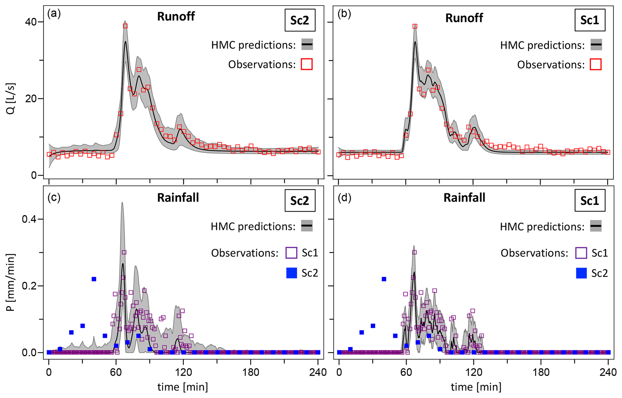
Figure 5 Comparison of observed and predicted discharges (a, b) and rainfall (c, d), based on Sc2 (a, c) and Sc1 (b, d) data. Predictions are represented by the median (black line) of the corresponding inferred distributions and a confidence interval given by the 2.5 and 97.5 percentiles (grey area). In the bottom panels the predicted rain is compared with both the inaccurate data of Sc2 (filled squares) and the accurate data of Sc1 (open squares).

The observed output peaks are used by the HMC algorithm as an additional source of information about the rain falling over the catchment area during the observation time. This new information, together with the stochastic input model, is used to attempt a reconstruction of a true rainfall pattern. The simulated rainfall and outflow patterns are represented by the medians of their inferred distributions (black line) and an uncertainty given by the 2.5 %–97.5 % quantiles (grey area). The rainfall pattern reconstructed using the inaccurate data of Sc2 (lower left panel) clearly displays the peaks corresponding to the rainfall events that had been missed by the pluviometer P2 located away from the catchment (filled blue squares). Such predicted peaks reproduce the rainfall events detected in Sc1 by the rain gauges P1_a and P1_b in the proximity of the area of interest (open purple squares) very accurately in both time and duration.

The right panels of Fig. 5 compare runoff and precipitation observations with the inferred discharge and rainfall patterns in the accurate framework of Sc1. Although the simulated rain in Sc1 features somewhat less intense peaks than in Sc2, the remarkable fact that emerges from the comparison of the left and right panels of Fig. 5 (referring to Sc2 and Sc1, respectively) is that the rainfall patterns predicted in the two scenarios are qualitatively very similar, despite the significant difference in the accuracy of the data used for the inference.

Although not shown here, we have also run the HMC inference without rainfall data at all, i.e. omitting the term f(P_obs∣ξ, σ_ξ) in the posterior density, obtaining both model parameter marginals and a predicted rainfall pattern that are substantially identical to those obtained with the inaccurate data of Sc2. Essentially, in Sc2 the HMC algorithm “learns” that the observed rain is unreliable and should thus be ignored. However, in most applications, the accuracy and reliability of the measured precipitation data is unknown a priori. In those cases the rainfall observations can be safely used in the inference process, since the algorithm itself will assess its accuracy and possibly disregard it in favour of a more reliable reconstructed rainfall.

The inferred outflows, shown in the upper panels of Fig. 5 match the observations very well and are essentially identical, compatible with the assumption that runoff data are accurate and the same for the two scenarios.

5 Conclusions

The goal of this work is to demonstrate that HMC algorithms employing a timescale separation can solve hard inference problems with stochastic hydrological models. In Albert et al. (2016) we proposed a novel implementation of an HMC algorithm combined with a multiple timescale integration for Bayesian parameter inference with nonlinear SDE models, and we demonstrated the performance of the method using a rainfall-runoff toy model with synthetic data time series. This work is the first application to a real-world case study, with real time series of measured rainfall and outflows. We show that the HMC algorithm is a powerful inference method for the data-driven calibration of hydrological model parameters, especially well suited for both computationally expensive stochastic models and cases, far from rare in hydrology, where the precipitation data are inaccurate and unreliable.

The combined SIP-HMC method presented here allows us also to estimate the “true” average rain input to a hydrological system in the case of highly inaccurate precipitation data probabilistically and with great accuracy, using only prior knowledge and the observed outflow. Runoff data are used by the algorithm as a first-hand information resource about the unknown precipitation over the catchment. This information can override the available, and possibly inaccurate, rainfall data. The reconstructed precipitation is then used to infer the hydrological model parameters, which are thus protected from the deteriorating effect of the uncertainty on the rainfall observations. This approach considerably reduces the bias in the inferred parameters and therefore leads to more reliable runoff predictions, which can in turn be very useful for decision-makers in planning and policy-making.

The use of AD makes the algorithm in principle applicable to more complex models. Indeed, the generalization of the algorithm from the toy model used in Albert et al. (2016) presented only one possibly challenging requirement, namely rewriting the Hamiltonian ℋ_HMC, while the rest of the implementation of the algorithm remained essentially unchanged. This application shows that ≈10³ parameters can be inferred in less than 2 h. This leaves us with a considerable margin to tackle more complex problems and datasets of much larger sizes. However, it must be noted that the HMC algorithm in the form described in this work is limited to non-spatially resolved models depending only on a time variable. In principle, the method could cope with further spatial dimensions, for example, describing inundations, but this would require a non-trivial adaptation of the algorithm, which is not discussed here. More importantly, a significant limitation of the HMC method presented in this work is that it requires, unlike methods that only involve forward-solving the model, such as SIP (Del Giudice et al., 2016), an explicitly discretized solution of the hydrological model (see Eq. 5), which might not be always easily available. In those cases, one may need to resort to appropriate numerical solvers, often employing advanced implicit schemes, which in turn may make AD problematic.

The extension of the HMC method described here to further hydrological models and systems will be the focus of future works. Furthermore, the HMC algorithm presented here is not at all limited to hydrology. It is a very general, efficient, easily parallelizable and scalable algorithm that makes Bayesian inference with expensive stochastic models feasible in spite of its computational hardships, with a very broad range of potential applications in applied sciences that can benefit from stochastic modelling and a fast Bayesian inference method.