Assessment of the interactions between soil–biosphere–atmosphere (ISBA) land surface model soil hydrology, using four closed-form soil water relationships and several lysimeters

Soil water drainage is the main source of groundwater recharge and river flow. It is therefore a key process for water resource management. In this study, we evaluate the soil hydrology and the soil water drainage, simulated by the interactions between soil–biosphere–atmosphere (ISBA) land surface model currently used for hydrological applications from the watershed scale to the global scale, where parameters are generally not calibrated. This evaluation is done using seven lysimeters from two long-term model approach sites measuring hourly water dynamics between 2009 and 2019 in northeastern France. These 2 m depth lysimeters are filled with different soil types and are either maintained as bare soil or covered with vegetation. Four closed-form equations describing soil water retention and hydraulic conductivity functions are tested, namely the commonly used equations from Brooks and Corey (1966) and van Genuchten (1980), a combination of the van Genuchten (1980) soil water retention function with the Brooks and Corey (1966) unsaturated hydraulic conductivity function, and, for the very first time in a land surface model (LSM), a modified version of the van Genuchten (1980) equations, with a new hydraulic conductivity curve proposed by Iden et al. (2015). The results indicate good performance by ISBA with the different closure equations in terms of soil volumetric water content and water mass. The drained flow at the bottom of the lysimeter is well simulated, using Brooks and Corey (1966), while some weaknesses appear with van Genuchten (1980) due to the abrupt shape near the saturation of its hydraulic conductivity function. The mixed form or the new van Genuchten (1980) hydraulic conductivity function from Iden et al. (2015) allows the solving of this problem and even improves the simulation of the drainage dynamic, especially for intense drainage events. The study also highlights the importance of the vertical heterogeneity of the soil hydrodynamic parameters to correctly simulate the drainage dynamic, in addition to the primary influence of the parameters characterizing the shape of the soil water retention function.

1 Introduction

Drainage water is the portion of precipitation that flows through the first metres of soil. As it has escaped evapotranspiration, it is the main diffuse source of groundwater recharge (Moeck et al., 2020) and is of crucial importance for estimating the evolution of an aquifer (Bredehoeft, 2002; Döll and Fiedler, 2008). Even where there is no aquifer, this water flux can contribute to the baseflow. Despite their importance, direct observations of drainage water are still rare compared to direct observations of river flow or groundwater level.

Indirect methods based on an analysis of baseflow (Meyboom, 1961) or a variation in the piezometric level, for instance, using a water table fluctuation method (Healy and Cook, 2002), can be applied to estimate groundwater recharge. However, these methods cannot separate the different components of the recharge, such as the exchange between surface water and groundwater (Brunner et al., 2017; Keshavarzi et al., 2016), exchanges between several aquifer layers basins (Tavakoly et al., 2019), and drainage water. Direct measurement at the local scale and at a high frequency can be made in situ, using lysimeter columns, which isolate a small volume of soil from the lateral flow and collect drainage water. Most of the time, the lysimeters are disconnected from the soil and avoid the capillary rise from the deeper soil that can have an important influence locally (Vergnes et al., 2014; Maxwell and Condon, 2016). From such observations, drainage water is known to have large variations in space, due to changes in soil texture and structure (Vereecken et al., 2019; Moeck et al., 2020).

Due to the limited number of observations and the difficulty around indirectly quantifying it, the estimation of the groundwater recharge is 1 of the 23 unsolved problems in hydrology (Blöschl et al., 2019). The simulation of recharge in hydrological models can vary significantly, from simplified reservoir approaches to physically based models. The widely used reservoir approach (Alcamo et al., 2003; Harbaugh, 2005) has the advantage of limiting the number of parameters to be calibrated and reducing the numerical cost of simulations. Physically based approaches are more complex and are commonly used in land surface models (LSMs) in which vertical water and energy balances between the land surface and the atmosphere can be calculated (De Rosnay et al., 2003; Blyth et al., 2010; Boone et al., 2000).

Today, LSMs are widely used in hydrological applications in order to study the regional and global water cycle, predict streamflow, and inform water resource management (Haddeland et al., 2011; Vincendon et al., 2016; Schellekens et al., 2017; Gelati et al., 2018; Le Moigne et al., 2020; Vergnes et al., 2020; Muñoz-Sabater et al., 2021; Rummler et al., 2022). In this context, the challenge of LSMs is finding a compromise between a simple application and an application that is powerful enough to reproduce the full water cycle. For example, in the unsaturated zone, hydrodynamic parameters are generally uncalibrated and are estimated with soil properties (Decharme et al., 2011, 2019; Le Moigne et al., 2020). However, LSMs may have difficulty estimating the dynamics of groundwater recharge, particularly during intense precipitation events. Vereecken et al. (2019) suggested a number of directions for improvement, namely introducing more physical processes such as preferential flow along the roots and macropores, improving the representation of the soil and vegetation and of soil parameters, and improving the spatiotemporal distribution of precipitation. In LSMs, the Richards (1931) equation is used to describe the flow of water in the porous soil due to the actions of capillarity and gravity. Mainly used in the hydrology community, this equation has been widely criticized, in particular for the overestimation of the effect of capillarity (Nimmo, 2010; Farthing and Ogden, 2017).

In the Richards (1931) equation, two closed-form equations, namely Brooks and Corey (1966) and van Genuchten (1980), hereafter BC66 and VG80, respectively, are often used to represent the variations in the volumetric water content with the matrix potential and the hydraulic conductivity in the unsaturated zone. Historically, the closed-form equations from BC66 are mostly used by the atmospheric community in theirs LSMs, while the ones from VG80 are mainly used by hydrologists. BC66 proposed the simple analytical power curves of soil water retention and hydraulic conductivity, based on North American soil observations. However, they do not include an inflection point close to saturation and are thus not derivable, leading to problems at the connection with the saturated zone. The consequence is a deviation near the saturation of volumetric water content. VG80 proposed an improvement of the BC66 soil water retention curve close to water saturation, using more complex analytical forms that are based on European soil observations. However, as summarized by Iden et al. (2015), when such an S-shaped function is used to described fine-textured soil or a soil with a wide pore size distribution, the VG80 hydraulic conductivity curve exhibits an abrupt drop at the transition from saturated conditions to unsaturated conditions. This may lead to underestimations of the hydraulic conductivity for very wet conditions, i.e. near saturation, and impact the stability and the accuracy of the numerical solver (Vogel et al., 2000; Ippisch et al., 2006). The nonlinear form also increases the cost of the numerical solvers (van Genuchten, 1980; Vogel et al., 2000; Ippisch et al., 2006; Dourado Neto et al., 2011).

To smooth the artefacts associated with the VG80 hydraulic conductivity curve, some studies suggest different solutions, such as shifting the entire pore size distribution with an air entry value (Kosugi, 1994), truncating the pore size distribution by introducing a maximum pore radius on the VG80 hydraulic conductivity curve (Schaap and Van Genuchten, 2006; Iden et al., 2015), or putting an explicit air entry pressure in the VG80 model (Fuentes et al., 1992; Braud et al., 1995; Vogel et al., 2000; Ippisch et al., 2006). Fuentes et al. (1992) or Braud et al. (1995) proposed combining the VG80 soil water retention function with the BC66 hydraulic conductivity curve. Such a combination should improve the simulation when the soil water is close to saturation, while preserving the simplicity and numerical stability of the BC66 relationships. It benefits from the many methods that link soil parameters from one relationship to another (van Genuchten, 1980; Lenhard et al., 1989). Recently, an elegant parametrization was proposed by Iden et al. (2015), which allows us to keep the VG80 hydraulic conductivity curve by introducing the concept of maximum pore radius, as suggested by Durner (1994).

The goal of this study is to use a state-of-the-art LSM to assess the benefits of the BC66 and VG80 relationship and two of its derivatives in reproducing soil water mass, volumetric water content, and drainage flux observed in seven lysimeters during more than 5 years. The two alternative approaches are (i) the one proposed by Fuentes et al. (1992) and Braud et al. (1995) that combines the VG80 soil water retention curve with the BC66 unsaturated hydraulic conductivity curve and (ii) the new parameterization of the VG80 hydraulic conductivity curve from Iden et al. (2015) that has never been used in an LSM, to the best of our knowledge. The soil hydrodynamic parameters are directly derived from observations and compared with several pedotransfer functions (hereafter PTFs) commonly used by LSMs. The LSM used is the multi-layer diffusion version of the interactions between soil–biosphere–atmosphere (ISBA) that directly solves the mixed form of the Richards (1931) equation (Boone et al., 2000; Decharme et al., 2011). The experimental protocol, including descriptions of both the lysimeter data and the ISBA model, is given in Sect. 2. Soil parameter estimation based on lysimeter observations is described in Sect. 3, while the main results of each model approach are presented in Sect. 4. Finally, a general discussion and the main conclusions are given Sect. 5.

2 Experimental protocol

2.1 Data

Seven lysimeters from two French experimental sites located in northeastern France are used in this study. There are three lysimeters from the GISFI experimental station (French Scientific Interest Group – Industrial Wasteland) at Homécourt (49^∘21^′ N, 5^∘99^′ E; altitude 430 m), with a data record from 2009 to 2016 (hereafter G1, G2, G3, and G4), and three lysimeters from OPE experimental station (Perennial Environmental Observatory) close to Osne-le-Val (48^∘5092^′ N, 5^∘2119^′ E; altitude 224 m), with a data record from 2014 to 2019 (hereafter O1, O2, and O3). These two sites are separated by a distance of 97 km. Their soils are classified according to the World Reference Base for Soil Resources (WRB; Hazelton and Murphy, 2016). For the lysimeters, the rain intercepted by the vegetation is assumed to evaporate or to eventually reach the ground, as this is the case for all natural surfaces with a vegetation canopy.

The GISFI experimental station focuses on the understanding of pollution evolution and the development of decontamination solutions (Lemaire et al., 2019; Huot et al., 2015; Rees et al., 2020; Ouvrard et al., 2011). It participates in the collaborative study of TEMPOL (Observation sur le long TErMe de sols POLlués) with the German observatory infrastructure of TERENO (Terrestrial Environmental Observatories; Zacharias et al., 2011) in order to study in situ the transfer of pollutants (Leyval et al., 2018). Three of the GISFI lysimeters (G1, G2, and G3) contain rebuilt soil of the Spolic toxic Technosol, which was sampled in Neuves-Maisons, an industrial wasteland of a coking plant with contamination (polycyclic aromatic hydrocarbons (PAHs) and hydrocarbons; Monserie et al., 2009; Ouvrard et al., 2011; Sterckeman et al., 2000). These three lysimeters were filled in September 2007 and the soil material was gradually and manually compacted every 0.3 m to reach a given bulk density. Lysimeters G1 and G2 were maintained as bare soil, while lysimeter G3 was covered by vegetation (alfalfa). Lysimeter G4 was filled by a monolith of Cambisol from Noyelles-Godault and covered by grass (Table 1).

Table 1 Description of each lysimeter, including the filling method, soil type, vegetation cover, number of texture observations, and textures (in percent of clay, sand, and silt) at different depths.

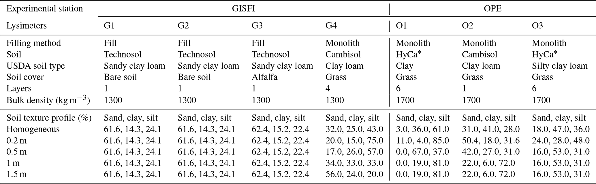
^* Hypereutric Cambisol.

The main objective of the OPE site is to describe the environment before and after the construction of the surface facilities of a deep radioactive waste repository and to follow its evolution. This site is part of the OZCAR (Observatoires de la Zone Critique: Application et Recherche) French research infrastructure dedicated to the observation and study of the critical zone (Gaillardet et al., 2018; Braud et al., 2020). The lysimeters were filled by monoliths taken close to the OPE site; lysimeters O1 and O3 were filled with hypereutric Cambisol, with different layers of limestone (more or less cracked), and lysimeter O2 contains a Cambisol. These three lysimeters had sparse vegetation composed of C3-type grass (Table 1). Monolith filled lysimeters preserve original soil horizons and are therefore better representative of watershed conditions.

All of the lysimeters are weighable cylinders, with a depth of 2 m and an area of 1 m². No suction is imposed at the bottom of each lysimeter, contrary to the ones used for TERENO-SOILCan (Putz et al., 2016). They are equipped with suction and temperature probes, in addition to time domain reflectometry (TDR) probes to measure the water content, at 0.50, 1.0, and 1.5 m depth, with an additional measurement at 0.2 m for the OPE lysimeters. The weight is measured continuously with a 0.1 kg precision, giving an idea of the time variations in the total soil water volume in the column, and a tipping counter measures the drainage water at the bottom. Data are continuously monitored on an hourly basis using a data logger. On the GISFI site, TDR probes are TRIME-PICO 32 sensors with internal TDR electronics. They are set horizontally and record the water content (in cm³ cm⁻³) on an hourly basis. The calibration is performed on two measurements, namely one in a dry condition and one in a water-saturated condition. At the OPE site, the soil moisture sensors used (UMP-1; Umwelt-Geräte-Technik GmbH) are based on a frequency domain reflectometry (FDR) method and measure the local change in dielectric permittivity. The tipping bucket resolution is 0.1 mm h⁻¹ at the two sites.

The sets of atmospheric forcing variables (wind speed, precipitation rate, short-wave incident radiation, air temperature, air humidity, and atmospheric pressure) used to force the ISBA LSM are observed in situ at an hourly time step by two local meteorological stations (one at OPE and one at GISFI). The atmospheric forcing is assumed to be identical for all of the lysimeters at each site. Annual precipitation is 20 % higher at the OPE site (876 mm yr⁻¹) than at the GISFI experimental station (727 mm yr⁻¹). Long-wave radiation is derived from atmospheric conditions, using the equation of Prata (1996). Atmospheric data gaps are filled by regressions on available data, using two neighbouring meteorologic stations. The gaps represent up to 12 % of the observations for the GISFI site.

All soils for all of the lysimeters are described in Table 1, while all available observations and their characteristics are summarized in Table S2.

2.2 ISBA model

The ISBA LSM was originally scheduled for use in numerical weather prediction and climate models. During the last few decades, ISBA has evolved from a simple bucket force–restore model (Noilhan and Planton, 1989) to a more explicit soil multi-layer diffusion scheme (Boone et al., 2000; Decharme et al., 2011) coupled with a snow multi-layer scheme of intermediate complexity (Boone and Etchevers, 2001; Decharme et al., 2016). ISBA is currently used in hydrological applications, especially to estimate groundwater recharge when it is associated with hydrologic models at both regional (Le Moigne et al., 2020; Tavakoly et al., 2019; Vergnes et al., 2020) and global scales (Vergnes and Decharme, 2012; Decharme et al., 2019). Several studies showed the good performance of ISBA in simulating field sites (Calvet et al., 1998; Boone et al., 2000; Decharme et al., 2011; Joetzjer et al., 2015; Garrigues et al., 2015, 2018; Morel et al., 2019).

The surface temperature evolves with the heat storage in the soil–vegetation composite and the thermal gradient between surface and the other layers (Boone et al., 2000; Decharme et al., 2011). At depth, the heat transfer is described by the use of the one-dimensional Fourier law. The soil heat capacity is the sum of the water heat capacity and the heat capacity of the soil. The soil thermal conductivity is a function of volumetric water content and porosity. Freezing due to water phase changes in the soil can also be computed by taking into account the effect of the sublimation of frost and the isolation of vegetation at the surface (Decharme et al., 2016).

ISBA simulates the land surface evapotranspiration as being the sum of the bare-soil evaporation, the soil freezing sublimation, the plant transpiration, the direct evaporation of the precipitation intercepted by the plant canopy, and the snow sublimation (Noilhan and Planton, 1989). Water for bare-soil evaporation is drawn from the first layer of the soil. This soil evaporation is weighted by the relative humidity of this superficial layer (Mahfouf and Noilhan, 1991). This relative humidity evolved nonlinearly with the superficial water content, potentially allowing the moisture content of the soil evaporation to be greater than the usual water content at the field capacity, which is specified as the matric potential at −0.33 bar. Plant transpiration is proportional to a stomatal conductance computed using an interactive vegetation scheme. The water used for transpiration is removed throughout the root zone in which the roots are asymptotically distributed, according to Jackson et al. (1996). Plant transpiration stops when the root zone water content is below the usual water content at wilting point, corresponding to a matric potential of −15 bar.

The interactive vegetation scheme of ISBA activated in this study represents 16 broad types of vegetation. The scheme represents plant photosynthesis and respiration, plant growth, and decay. The simulated stomatal conductance depends on photosynthesis and controls transpiration. The vegetation canopy is characterized by the leaf area index (LAI), which results directly from the carbon balance computation of the leaves. The simulated LAI varies during the year, according to photosynthetic activity, respiration, and decay. In spring, for instance, when photosynthetic activity is high due to high solar radiation and sufficient volumetric water content, the LAI increases. LAI affects the transpiration and the evaporation of water on the canopy associated with intercepted rain or dew deposition. Photosynthesis and respiration are parameterized, according to the semi-empirical model of Goudriaan et al. (1985), and implemented by Jacobs et al. (1996) and Calvet et al. (1998). Plant growth and decay are based on Calvet and Soussana (2001), Gibelin et al. (2006), and Joetzjer et al. (2015). A complete description of the carbon cycle in vegetation can be found in Delire et al. (2020).

In ISBA, the intercepted rain by vegetation is fully represented and based on a simple rainfall interception scheme (Noilhan and Planton, 1989; Noilhan and Mahfouf, 1996). The interception reservoir is fed by the intercepted rain by vegetation. When this reservoir is larger than its maximum value (equal to 0.2xLAI), then the dripping from the vegetation is computed as a simple mass balance. The direct evaporation of the vegetation is drawn from this interception reservoir and depends on the fraction of the foliage covered by intercepted water, as proposed by Deardorff (1978).

The ISBA soil hydrology uses the following mixed form of the Richards (1931) equation to describe the water mass transfer within the soil via Darcy's law:

$$\begin{array}{}\text{(1)}& {\displaystyle \frac{\partial \mathit{\omega }\left(z\right)}{\partial t}}={\displaystyle \frac{\partial }{\partial z}}\left[-k\left(z\right)\left({\displaystyle \frac{\partial \mathit{\psi }\left(z\right)}{\partial z}}+\mathrm{1}\right)\right]+{\displaystyle \frac{S\left(z\right)}{{\mathit{\rho }}_{\mathit{\omega }}}},\end{array}$$

where ω (m³ m⁻³) is the volumetric water content at each depth z (m), ψ (m) ia the water pressure head, and k (m s⁻¹) is the soil hydraulic conductivity. S (kg m⁻³ s⁻¹) is the soil water source/sink term related to water withdrawn by evapotranspiration in each layer. A complete description of the model equations used to simulate water transport can be found in Boone et al. (2000) and Decharme et al. (2011, 2019). This soil hydrology is solved numerically, using a Crank–Nicolson time scheme, where the flux term is linearized via a first‐order Taylor series expansion. The resulting linear set of diffusion equations can be cast in a tridiagonal form and solved quickly (see Sect. S1 in the Supplement for more details). The soil discretization is adapted to the lysimeter depth and to the measurement depths for which 14 soil layers are used at 0.01, 0.04, 0.1, 0.2, 0.4, 0.6, 1.0, 1.2, 1.4, 1.6, 1.8, 1.95, and 2 m depths. ISBA uses the soil infiltration at the surface as upper boundary condition, neglecting the surface runoff when simulating local field or lysimeter sites. This soil infiltration is the flux of water reaching the soil surface (i.e. the sum of the precipitation not intercepted by the canopy, the dripping from the vegetation, and the snowmelt). At the bottom of the soil column, a fine layer of 5 cm is used to simulate a seepage face lower boundary condition (LBC) instead of the usual free-drainage LBC used in ISBA (see Sect. S1.3). Such a seepage face LBC is recommended to simulate the lysimeters (Séré et al., 2012; Tifafi et al., 2017). Finally, to compute the initial conditions, a spin-up of 1 year is done, using the first year of each forcing dataset in order to ensure an adequate numerical equilibrium for soil water.

2.3 Model approaches

In this study, we evaluate four closed‐form equations that link the volumetric water content, soil matric potential, and hydraulic conductivity, assuming a residual water content (ω_r) equal to 0. All simulations use the same ISBA configuration and are denoted as follows:

• BC66. This first model approach uses the standard version of ISBA, i.e. the closed‐form equations of Brooks and Corey (1966), where the soil water retention function, ψ(ω), and the hydraulic conductivity function, k(ψ), are given by the following:

  $$\begin{array}{}\text{(2)}& \left\{\begin{array}{l}\mathit{\psi }\left(\mathit{\omega }\right)={\mathit{\psi }}_{\mathrm{sat}}{\left(\frac{\mathit{\omega }}{{\mathit{\omega }}_{\mathrm{sat}}}\right)}^{-b}\\ k\left(\mathit{\psi }\right)=k_{\mathrm{sat}}{\left({\displaystyle \frac{\mathit{\psi }}{{\mathit{\psi }}_{\mathrm{sat}}}}\right)}^{-\frac{\mathrm{2}b+\mathrm{3}}{b}}\end{array}\right.,\end{array}$$

  where b (–) represents the dimensionless shape parameter of the soil water retention function, while ψ_sat (m) and k_sat (m s⁻¹) are the soil matrix potential and hydraulic conductivity at saturation, respectively.

• VG80. This second model approach uses the following closed‐form equations from van Genuchten (1980), using the Mualem (1976) theory:

  $$\begin{array}{}\text{(3)}& \left\{\begin{array}{l}\mathit{\psi }\left(\mathit{\omega }\right)=-\frac{\mathrm{1}}{\mathit{\alpha }}{\left[{\left(\frac{\mathit{\omega }}{{\mathit{\omega }}_{\mathrm{sat}}}\right)}^{-\mathrm{1}/m}-\mathrm{1}\right]}^{\mathrm{1}/n}\\ \mathrm{with}m=\mathrm{1}-\frac{\mathrm{1}}{n}\\ k\left(\mathit{\psi }\right)=k_{\mathrm{sat}}\cdot S^l[\mathrm{1}-(\mathrm{1}-S^{\mathrm{1}/m}{)}^m{]}^{\mathrm{2}}\\ \mathrm{with}S={\left[\mathrm{1}+|\mathit{\alpha }\mathit{\psi }{|}^n\right]}^{-m}\end{array}\right.,\end{array}$$

  where α (m⁻¹) is the inflection point at which the slope of the soil water retention function ($\mathrm{d}\mathit{\omega }/\mathrm{d}\mathit{\psi }$) reaches its maximum value, n (–) is a dimensionless coefficient that characterizes the shape of the retention curve, and l is the Mualem (1976) dimensionless parameter that determines the slope of the hydraulic conductivity function.

• BCVG. This third model approach (see Fuentes et al., 1992, or Braud et al., 1995) uses a combination of the ψ(ω) function from VG80 with the k(ψ) function from BC66, using the Burdine (1953) theory as follows:

  $$\begin{array}{}\text{(4)}& \left\{\begin{array}{l}\mathit{\psi }\left(\mathit{\omega }\right)=-\frac{\mathrm{1}}{\mathit{\alpha }}{\left[{\left(\frac{\mathit{\omega }}{{\mathit{\omega }}_{\mathrm{sat}}}\right)}^{-\mathrm{1}/m_b}-\mathrm{1}\right]}^{\mathrm{1}/n_b}\\ \mathrm{with}{m}_b=\mathrm{1}-\frac{\mathrm{2}}{n_b}\\ k\left(\mathit{\psi }\right)=k_{\mathrm{sat}}\cdot S_b^{\mathrm{2}{\mathit{\lambda }}_b+\mathrm{3}}\\ \mathrm{with}{\mathit{\lambda }}_b={\left(n_b-\mathrm{2}\right)}^{-\mathrm{1}}\mathrm{and}{S}_b={\left[\mathrm{1}+|\mathit{\alpha }\mathit{\psi }{|}^{n_b}\right]}^{-m_b}\end{array}\right.,\end{array}$$

  where n_b (–) is the dimensionless coefficient that characterizes the shape of the retention curve using Burdine (1953) theory.

• VGc. This last approach uses the usual ψ(ω) function from VG80 in Eq. (3) and the corrected form of the k(ψ) function from Iden et al. (2015), using the Mualem (1976) theory as follows:

  $$\begin{array}{}\text{(5)}& k\left(\mathit{\psi }\right)=k_{\mathrm{sat}}{\displaystyle \frac{S^l}{{\mathrm{\Gamma }}^{\mathrm{2}}}}\cdot \left\{\begin{array}{ll}{\left[\mathrm{1}-{\left(\mathrm{1}-S^{\mathrm{1}/m}\right)}^m\right]}^{\mathrm{2}}& \forall \mathit{\psi }\le {\mathit{\psi }}_c\\ {\left[\mathrm{1}-{\left(\mathrm{1}-S_c^{\mathrm{1}/m}\right)}^m+{\displaystyle \frac{S-S_c}{\left|\mathit{\alpha }{\mathit{\psi }}_c\right|}}\right]}^{\mathrm{2}}& \forall \mathit{\psi }>{\mathit{\psi }}_c\end{array}\right.,\end{array}$$

  with $S_c=[\mathrm{1}+|\mathit{\alpha }{\mathit{\psi }}_c{|}^n{]}^{-m}$ and $\mathrm{\Gamma }=\mathrm{1}-(\mathrm{1}-S_c^{\mathrm{1}/m}{)}^m+\frac{\mathrm{1}-S_c}{\left|\mathit{\alpha }{\mathit{\psi }}_c\right|}$, where ψ_c (m) is the value of the maximum suction near saturation. It is fixed at −0.01 m, as suggested by Iden et al. (2015), which is equivalent to use a maximum pore size only in the capillary bundle model.

Additional sensitivity tests were made (see Sect. 5) first to compare the impact of prescribing homogeneous soil profiles, which are classically derived from the use of pedological soil maps, versus heterogeneous soil profiles, which are generally observed in situ. Second, we test the performances of using soil parameter values derived from the usual PTFs (Clapp and Hornberger, 1978; Cosby et al., 1984; Carsel and Parrish, 1988; Wösten and van Genuchten, 1988; Vereecken et al., 1989; Weynants et al., 2009) instead of using soil parameter values observed in situ. Finally, we also assess the impact of using the seepage face LBC compared to the usual free-drainage LBC used in ISBA over natural sites and in regional- and global-scale applications.

3 Estimation of parameters

3.1 Soil parameters

The rich datasets collected by the lysimeters (hourly resolution with 3220 observations on average by lysimeters and by depth) allow us to estimate the soil hydrodynamic parameters, such as in previous studies (Brooks and Corey, 1966; van Genuchten, 1980; Carsel and Parrish, 1988). For instance, Fig. 1 plots the observed soil water retention curves, namely the volumetric water content, ω, as a function of the logarithm of the absolute value of the soil matrix potential, ψ (dots with different colours for each depth) for lysimeters G2 and O1 (other lysimeters are given in Figs. S1 and S2 in the Supplement). To remove the effect of hysteresis on the observed soil water retention curves (i.e. the difference in soil water retention curve measured under wetting and drying process; Haines, 1930), we have averaged the ω values for each ψ values. Figure 1 reveals an important heterogeneity with depth. From these observed soil water retention curves, ω_sat, ψ_sat, α, n, n_b, and b can be derived at each depth of each soil column (for example, b is the slope of this relation). To this end, we use an objective least squares function, which minimizes the sum of the squares of the deviations. This function allows us to maximize the likelihood with a normal distribution (nls function in RStudio). The soil parameter estimates allow us to plot soil water retention curves from BC66 and VG80 (red and blue lines, respectively) in Fig. 1, showing a better fit for VG80 than BC66.

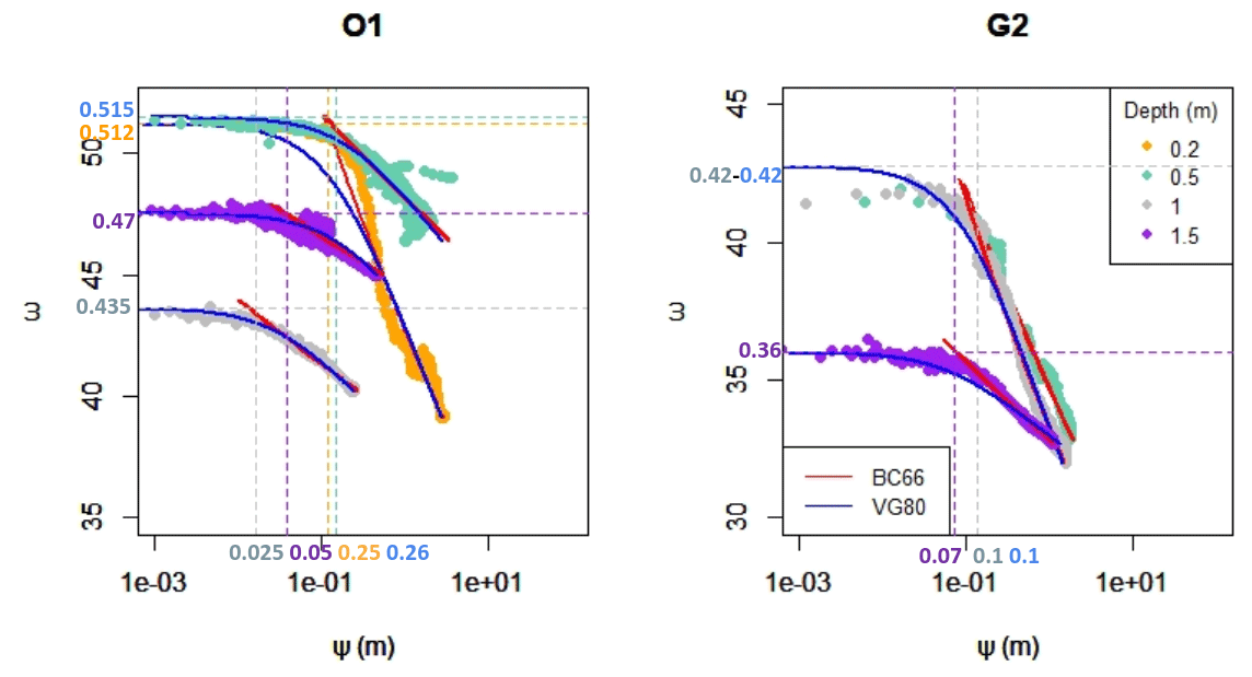
Figure 1 Soil water retention curves after removing the effect of hysteresis, with the volumetric water content (ω) and logarithm of the absolute value of the soil matric potential (ψ) for lysimeters O1 and G2. Observations at 0.2, 0.5, 1.0, and 1.5 m depth are represented by orange, aquamarine, grey, and purple diamonds, respectively, and estimations by red and blue dots for BC66 and VG80, respectively. The dashed lines are the estimated values via the observations for the water content at saturation and matric potential.

Next, we use two steps to evaluate this method and the soil parameter estimates. First, we successfully check that (1) the estimated ω_sat is consistent with the 99th percentile of the observed soil volumetric water content at each depth and for each lysimeter and that (2) the estimated n, n_b, and b or α and ψ_sat verify the following well-known relationships defined by van Genuchten (1980), as follows:

$$\begin{array}{}\text{(6)}& \left\{\begin{array}{ll}n\approx \mathrm{1}+b^{-\mathrm{1}}& \mathrm{for}\mathrm{Mualem}\mathrm{theory}\\ n_b\approx \mathrm{2}+b^{-\mathrm{1}}& \mathrm{for}\mathrm{Burdine}\mathrm{theory}\\ \mathit{\alpha }\approx |{\mathit{\psi }}_{\mathrm{sat}}{|}^{-\mathrm{1}}& \end{array}\right..\end{array}$$

Although several authors proposed more complex relationships that allow the preservation of the capillary effects (Lenhard et al., 1989; Morel-Seytoux et al., 1996; Leij et al., 2005; Sommer and Stöckle, 2010), a comparison of some of these relationships by Ma et al. (1999) has shown that the van Genuchten (1980) and Lenhard et al. (1989) relationships give better results. It is interesting to note that the simple relationship $n_b\approx n+\mathrm{1}$ is usually true for our soils (see Table S2). This justifies our choice to not represent the ω(ψ) relationship from BCVG (Eq. 4) in Fig. 1 (and thus in Figs. S1 and S2) because it is similar to the ω(ψ) relationship from VG80 (Eq. 3). Second, we compare our estimates to an alternative method to derive soil parameters from observed soil water retention curves based on the package SoilHyP (Dettmann et al., 2022), which uses the shuffled complex evolution (SCE) optimization. Soil parameter values found with this method are very close to our estimates, as shown by the low mean relative bias between both estimates (5 % for b, 1 % for n, 2 % for ω_sat, and 4 % for ψ_sat). Note that, for α, even if the mean relative bias seems to be not negligible (11 %), both estimates still remain very close (20.64 m⁻¹ on average for SoilHyP and 18.46 m⁻¹ for this study).

Estimations of the soil hydraulic conductivity function parameters (k_sat and l) are more difficult because of the lack of observed hydraulic conductivity profiles in each lysimeter. When the deepest part of each lysimeter is close to saturation, we assume that the soil hydraulic conductivity at saturation, k_sat, can be considered equal to the observed hourly drainage at 2 m depth. k_sat is thus derived empirically from the 99.9 percentile of the hourly drainage distributions. No assumption is made on a hypothetical k_sat profile with depth; i.e. k_sat is taken to be homogeneous with depth in each lysimeter. For VG80, a particular attention is also given to the very low n values for which Eq. (3) is numerically unstable. In this study, we found that our simulations are numerically stable when n≥1.1, so the limit of n is fixed at n=1.1. As already said, BCVG (Eq. 4) and VGc (Eq. 5) allow us to cancel this limitation. The l parameter in Eq. (3) for VG80 and Eq. (5) for VGc is estimated with a simple calibration via the ISBA sensitivity tests, with l ranging from −5 to 5. Better scores are obtained for l equal to 0.5, a classical value, for the OPE experimental station. For the GISFI experimental station, better scores are obtained for l equal to 0.5 (G4), −2 (G1 and G2), and −5 (G3), which remains consistent with the literature (Wösten and van Genuchten, 1988; Wösten et al., 2001; Schaap et al., 2001). We choose l to be constant over the entire soil profile for each lysimeter.

Figure 2 gives an example for lysimeters O1 and G2 of the relative soil hydraulic conductivity, $k/k_{\mathrm{sat}}$, as a function of the soil water content actual saturation, $\mathit{\omega }/{\mathit{\omega }}_{\mathrm{sat}}$, derived from the four closed-form equations described previously (other lysimeters are given in Fig. S3). The VG80 hydraulic conductivity exhibits an abrupt drop at the transition from saturated conditions to unsaturated conditions, contrary to BC66. This behaviour is well known for fine-textured soil as in our lysimeters (Fuentes et al., 1992; Vogel et al., 2000; Ippisch et al., 2006; Iden et al., 2015). This explains why the VG80 hydraulic conductivity function with small n values is strongly unstable near saturation. A comparison with the observed hourly drainage water at 2 m depth (reduced to k_sat) versus the actual saturation at 1.5 m depth seems to confirm that VG80 certainly underestimates the actual hydraulic conductivity near saturation for fine-textured soil, as underlined by previous studies (Vogel et al., 2000; Ippisch et al., 2006; Iden et al., 2015).

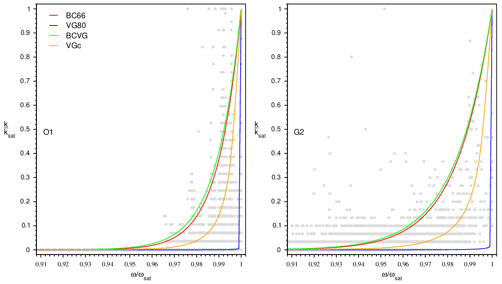
Figure 2 Near-saturation estimates of the relative soil hydraulic conductivity, $k/k_{\mathrm{sat}}$, as a function of the soil water content's actual saturation, $\mathit{\omega }/{\mathit{\omega }}_{\mathrm{sat}}$, for lysimeters O1 and G2 at 1.5 m depth. BC66 (red), VG80 (blue), BCVG (green), and VGc (orange) are computed using parameter estimates (Table S2) into Eqs. (2)–(5), respectively. The dots represent the observed hourly drainage water at 2 m depth (reduced to k_sat) versus the actual saturation at 1.5 m depth.

All parameter estimates are presented in Fig. 3 and in Table S2. Parameters vary greatly with depth (especially b, n, ψ_sat, and α) and, to a lesser extent, between lysimeters. n_b is not shown in Fig. 3 because it varies as n does. Although these heterogeneities can be observed on field sites, they could also be increased by factors like the compaction and structuration generally present in lysimeters (Weihermüller et al., 2007; Séré et al., 2012). The largest differences are found for b (and thus n). For all of the lysimeters, except G1 and G4, b increases with depth (and, conversely, n decreases). For the OPE lysimeters, b starts with 8 at 0.2 m depth, doubles twice (first at 0.5 m and then at 1 m depth), and then reaches 50 at 1.5 m. These variations are less pronounced for the GISFI lysimeters, with only a variation with depth by a factor of 2 for G2. The absolute value of ψ_sat decreases with depth (and, conversely, α increases), especially for the OPE lysimeters. Lysimeters were filled with preserved soil columns at the OPE and manually at the GISFI. Repacked soil columns are generally recognized as being more homogenous than undisturbed monoliths (Weihermüller et al., 2007; Carrick et al., 2017). The fact that the GISFI lysimeters are filled in a manual way can thus explain the weaker soil heterogeneities with depth, although they have been filled to preserve the bulk density of the soil.

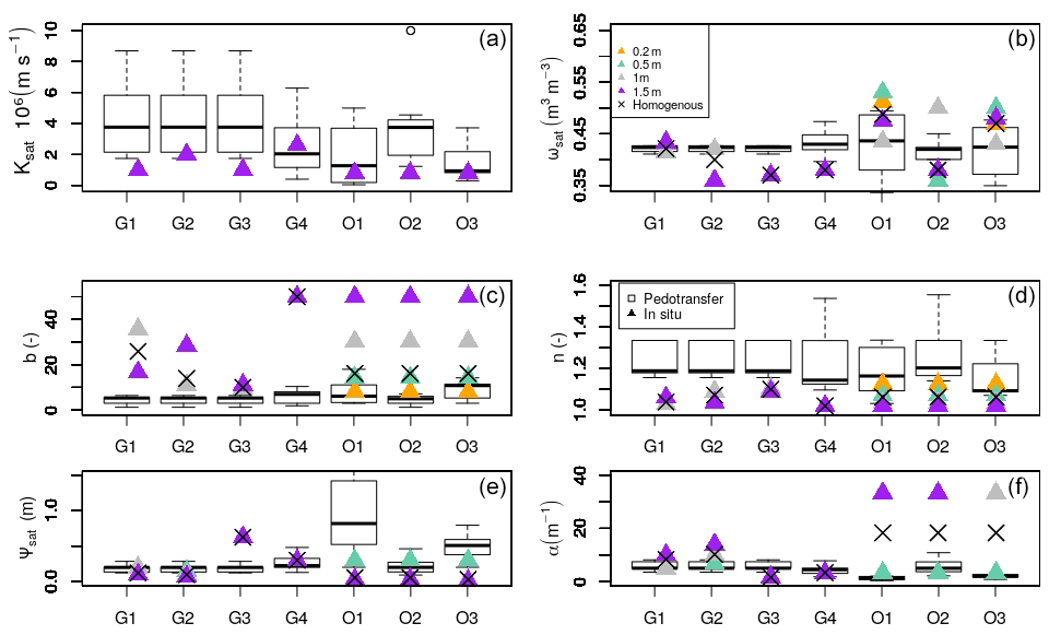
Figure 3 From left to right and top to bottom: the hydraulic conductivity at saturation, k_sat (10⁶ m s⁻¹), volumetric water content at saturation ω_sat (m³ m⁻³), b and n, matric potential at saturation, ψ_sat (m), and α (m). Estimations from in situ measurements are represented by triangles at 0.2, 0.5, 1, and 1.5 m (orange, aquamarine, grey, and purple, respectively), and their mean (homogeneous) values are represented by crosses (×). The values derived from the six pedotransfer function are shown by a box plot presenting the median, 25 %, and 75 % quantiles.

When comparing our parameter estimates to the PTFs usually used in LSMs (Clapp and Hornberger, 1978; Cosby et al., 1984; Carsel and Parrish, 1988; Wösten and van Genuchten, 1988; Vereecken et al., 1989; Weynants et al., 2009), we find that b (and thus n) from the in situ estimates are quite different from those determined by the PTFs (box plots). While b ranges from 5 to 12 with the usual PTFs, our estimates range from 8 to 50. ψ_sat (and thus α) estimates are slightly different from those determined by usual PTFs. For other parameters, our estimates and the usual PTFs give similar values.

3.2 Vegetation parameters

For the lysimeters covered by vegetation (O1, O2, O3, G3, and G4), two additional soil parameters must be determined. The field capacity ω_fc and the wilting point ω_wilt are computed via matrix pressure at −0.33 and −15 bar, respectively. The root depths have also been determined. Although the rooting depth was not measured at the sites, it is possible to derive it from the observations of the volumetric water content profile; if the volumetric water content presents a slow decrease in summer at a given depth, then it is considered that the roots have not yet reached this depth. The root depth is thus fixed at 2 m for lysimeters G3 and O2 and varies for lysimeters G4, O1, and O3. From 2009 to 2013, the root depth in lysimeter G4 reached 1.5 m; but after June 2013, seeding and harvesting were carried out every year, limiting roots whose development never reached below 0.4 m depth. In lysimeters O1 and O3, the root depth reached 0.8 m from 2014 to 2018 and 2 m thereafter. Standard ISBA values of maximum photosynthesis, leaf nitrogen content, and specific leaf area were used for the lysimeters covered by grass, but specific values were derived form the TRY database (Kattge et al., 2020) for alfalfa, as this crop is not a standard vegetation type in ISBA.

As there are no measurements of LAI for these lysimeters, the simulation of the LAI can only be compared to the literature. As expected, the simulated LAI is minimal between December and April and maximal in August, and there are variabilities between years (Fig. S4). For soils with grass (G4, O1, O2, and O3), the maximum LAI varies between 3 and 5, and the mean annual LAI varies between 1.3 and 2. These values are similar to those found in other studies (Calvet, 2000; Darvishzadeh et al., 2008). LAI for alfalfa cover (G3) is larger (LAI_max=7.5; LAI_mean=4.8), which is expected for such well-developed vegetation (Wolf et al., 1976; Wafa et al., 2018).

4 Results

Here, we present the main results for each model approach described in Sect. 2.3 in terms of simulated soil water and drainage water dynamics, water budget, and intense drainage water events. We used four skill scores to assess the ability of each model approach to reproduce the observation. These include the overall bias between the simulation and observation, the centred root mean square error (CRMSE) computed by subtracting the simulated and observed annual means from their respective time series before computing a standard root mean square error, the coefficient of determination (R²) or the Pearson correlation (R), and the Nash and Sutcliffe (1970) efficiency criterion (NASH) that determines the relative magnitude of the residual variance compared to the measured data variance. These scores are summarized in Appendix A. Note that the simulated soil temperatures have also been studied and analysed. All model approaches have shown that good skill scores (R²>0.9) underlie the ability of the ISBA LSM to reproduce observed soil temperatures. Because there are no significant differences between the four model approaches compared to the observations, these results are not presented in this study.

4.1 Soil water dynamics

The dataset allows the assessment of the evolution of the total soil water mass derived from the mass of the lysimeter, of the soil volumetric water content at several depths, and of the drainage water flux at the bottom of the lysimeters. In the following analysis, periods during which the meteorological forcing is reconstructed or when data are of poor quality (Table S1 in the Supplement) are not taken into account in the score computation. These periods are short, except for the drainage water of lysimeter G3 (23 % of the duration).

4.1.1 Water mass time variations

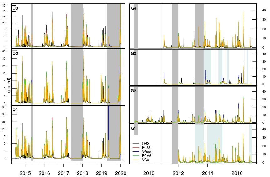
As there are no observations of the weight of the dry soil in each lysimeter that can serve as a reference, we evaluate the ability of ISBA to simulate the temporal variation in the water mass around the mean and not around the absolute mass of each lysimeter. These variations are assumed to be equal to the time variations in the total mass of the lysimeter, neglecting the seasonal variations in the vegetation mass. Time variations in the water masses are presented in Fig. 4 for the seven lysimeters at 1 h time step. All model approaches (BC66, VG80, BCVG, and VGc) are represented.

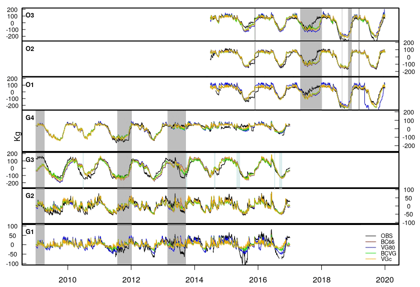
Figure 4 Hourly time series of the total water mass variations (kg) around the observed or simulated means from GISFI (G1, G2, G3, and G4) and OPE (O1, O2, and O3) lysimeters. Observations are in black, the BC66 model approach in red, VG80 in blue, BCVG in green, and VGc in orange. The grey shaded areas correspond to periods when the meteorological forcing is reconstructed and the blue shaded areas to the periods when data are of low quality.

With soil parameters determined in situ, the evolution of the total soil water mass is well reproduced by ISBA, whatever the model approach (Fig. 4). Skill scores (Fig. 5) are better for OPE experimental station lysimeters with a small CRMSE (below 56 kg, except for O1 with VG80). A comparison of the four model approaches shows that BC66, BCVG, and VGc exhibit better scores, with a mean CRMSE of 32, 32, and 34 kg, respectively, compared to 43 kg for VG80. VG80 also exhibits a lower R² (0.68), compared to other experiments (0.75, 0.75, and 0.72 for BC66, BCVG, and VGc, respectively).

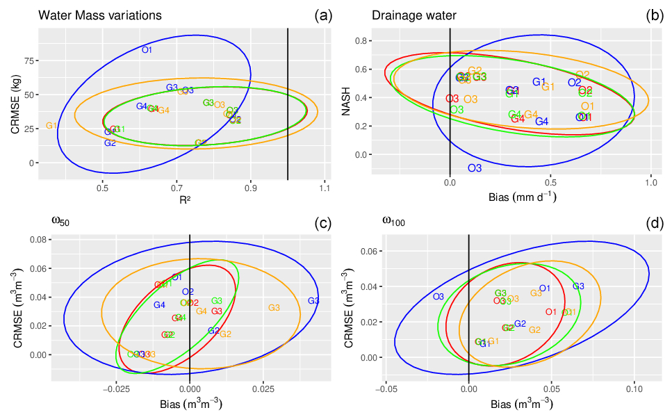
Figure 5 Statistical scores on daily chronicles reached by BC66 (red), VG80 (blue), BCVG (green), and VGc (orange). Panel (a) shows R² vs. CRMSE scores for the total water mass variations. Panels (c) and (d) show overall bias vs. CRMSE scores for the volumetric water content at 0.5 m depth (ω₅₀) and 1 m depth (ω₁₀₀), respectively. Panel (b) shows the overall bias vs. NASH scores for the drainage flux. All of these skill scores are presented in Appendix A. Each lysimeter is represented by its identifier. For each model approach, the ellipses represent the multivariate Student's t distribution, following Fisher (1992).

4.1.2 Water content

Time evolutions of the water content at 0.5 m are shown in Fig. 6, while the scores are presented for the two depths for which there are the most usable observations, i.e. 0.5 and 1 m (Fig. 5). For lysimeters with vegetation (G3, G4, O1, O2, and O3), the roots draw water in the summer period, which reduces the volumetric water content, causing a more pronounced contrast in the volumetric water content between winter and summer than for bare-soil lysimeters. This behaviour is well represented by ISBA because the biases are negligible ($<\mathrm{6}\times {\mathrm{10}}^{-\mathrm{2}}$ m³ m⁻³) and dynamics are correct (R²>0.5; not shown). Still, minor differences between BC66, BCVG, and VGc appear. VG80 obtains weaker statistical scores in 65 % of the cases because soil water saturation is reached too rapidly. VGc is clearly a solution for simulating the water content when the parameter n is close to 1, by correcting the default of VG80 for these soils.

Figure 6 Same as Fig. 4 but for hourly volumetric water content (m³ m⁻³) at 0.5 m depth.

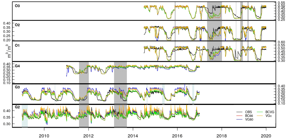
It should be noticed that the agreement between the observed and simulated soil volumetric water content is weaker at the shallow depth (available only at OPE; 0.2 m) compared to other depths with R²<0.6 (not shown). This can be explained by the different processes which can modify the structure of the soil at the surface; the intensity of precipitation can increase the soil surface sealing (Liu et al., 2011; Assouline, 2004), and the soil heterogeneity can increase in response to plant or biological activities (Brown et al., 2000; Beven and Germann, 1982). Such processes are not represented in ISBA.

4.1.3 Drainage water

Drainage at 2 m depth is measured at an hourly frequency. However, to compensate for the measurement limits associated with a 0.1 mm h⁻¹ threshold, the data are aggregated daily. The annual volume drained varies significantly between the lysimeters at the same sites (Table S2), although it is assumed that they are exposed to the same atmospheric conditions. At the GISFI experimental station, the mean annual drained water is at maximum levels for the bare-soil lysimeters G1 and G2 (>300 mm yr⁻¹). The mean annual drained water is 2 to 3 times lower for the lysimeters covered by vegetation. At the OPE experimental station, all the lysimeters have vegetation cover, and the mean annual drained water shows a variation of only 16 %, from 300 to 363 mm yr⁻¹. Such values are comparable to the volume drained on the bare soil of the GISFI experimental station, which is mainly due to the higher mean annual precipitation at OPE.

The daily mean annual cycles of drainage water are shown in Fig. 7. At the GISFI experimental station, drainage water occurs almost all year long for the bare-soil lysimeters G1 and G2. The well developed vegetation cover in G3 causes a decrease in both the drainage water intensity and drainage water duration. At the OPE experimental station, the drainage water occurs mainly from October to June (if the year 2016 is excluded, as a large rainfall event occurred in May–June 2016), with similar cycles for the three lysimeters. The annual cycle is well simulated, with more discrepancies for the VG80 model approach, which tends to overestimate the drainage water during some recession periods (as, for example, during spring for G1, G4, and O3).

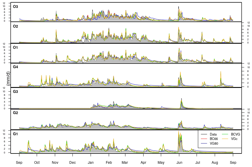
Figure 7 Same as Fig. 4 but for the daily mean annual cycles of the drainage water time series (mm d⁻¹).

The daily drainage water is shown in Fig. 8, and the scores are given in Fig. 5. Even if the annual volume drained is higher for the OPE lysimeters, the maximum drainage water intensities over the observed period are similar at both sites; they vary between 27.4 and 34.0 mm d⁻¹ at the OPE experimental station and between 24.0 and 33.0 mm d⁻¹ at the GISFI site. The four model approaches reproduce the daily drainage water with relatively low biases (<0.7 mm d⁻¹), with the worst biases being obtained by VG80, especially for the GISFI lysimeters, and confirming the results shown in Fig. 7. Dynamics are also well reproduced, as shown by the NASH scores. These scores are similar for BC66, BCVG, and VGc, with an average NASH of 0.42, 0.42, and 0.43, respectively, but with a slightly lower score, 0.35, for VG80. The worse performance of VG80 in reproducing the daily drainage water is especially true for the GISFI lysimeters.

Figure 8 Same as Fig. 4 but for daily drainage water (mm d⁻¹).

4.2 Water budget

Lysimeters give access to an estimate of the actual evapotranspiration (Schrader et al., 2013; Gebler et al., 2015). By neglecting the lateral runoff (not present in these lysimeters), the following simple water balance equation allows us to estimate annual evapotranspiration (E) from annual precipitation (P), annual drainage (Q_drain), and a water mass variation that is negligible (ΔW) for each lysimeter:

$$\begin{array}{}\text{(7)}& E=P-Q_{\mathrm{drain}}-\mathrm{\Delta }W.\end{array}$$

Figure 9 presents the water budget observed and simulated over the entire period for all lysimeters. The ratios of the total evapotranspiration and the drainage water to the total precipitation are expressed in percentages. At the GISFI experimental station, between 50 % and 80 % of the annual rainfall is evapotranspired, with maximal uptake for lysimeter G3, which has the densest vegetation cover. At the OPE experimental station, evapotranspiration corresponds to nearly 50 % of the rainfall.

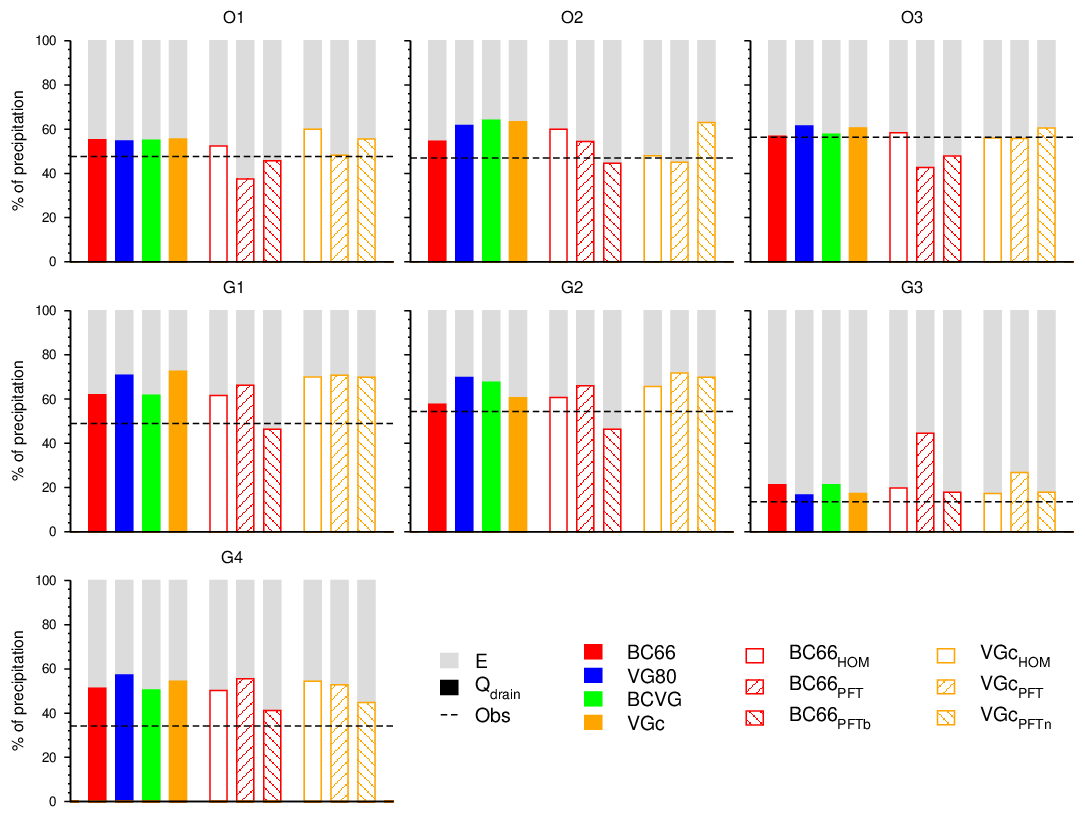
Figure 9 Water budget partition of the precipitation into drainage water and evapotranspiration (expressed in %) for lysimeters at GISFI (G1, G2, G3, and G4) and OPE (O1, O2, and O3) for each model approach. The ratio of observed drainage water to precipitation is represented by the dashed black line. Simulated drainage water is represented by colour bars for each model approach, while the simulated evapotranspiration (E) is shown in grey. The BC66 simulated drainage water is in red, VG80 in blue, BCVG in green, and VGc in orange. Drainage water simulated by additional model approaches with a homogeneous soil profile (BC66_HOM and VGc_HOM), with parameters estimated from usual PTFs (BC66_PTF and VGc_PTF), and with parameters estimated from the usual PTFs, except for b (B66${}_{{\mathrm{PTF}}_b}$) or n (VGc${}_{{\mathrm{PTF}}_n}$), estimated in situ are also shown. These last model approaches are defined in Sect. 5.

The annual budgets simulated by ISBA are rather close to the observations, but the drainage water is generally overestimated and thus the evapotranspiration underestimated on all lysimeters. The absolute difference averaged over all the lysimeters is not significant different between experiments. There are lower values for BC66 (8.1 percentage points) compared to the other model approaches (10.8 percentage points for BCVG, 11.7 for VGc, and 12.9 for VG80). This seems to underline that using the closed‐form equations from van Genuchten (1980) could favour drainage water at the expense of evapotranspiration, compared to Brooks and Corey (1966), at least over our lysimeters, and with the ISBA LSM.

4.3 Intense drainage events

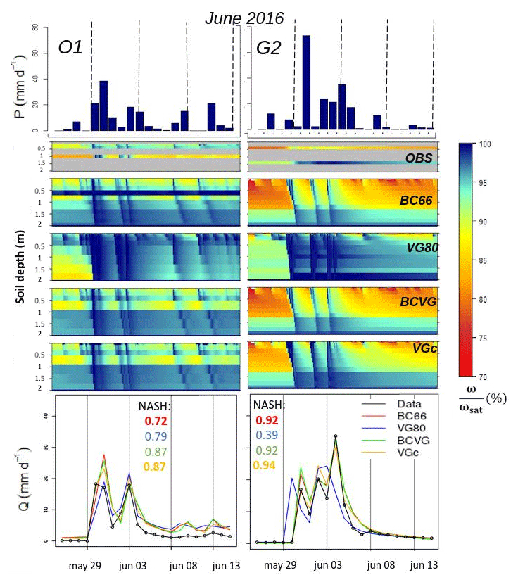
In the previous sections (Sects. 4.1.3 and 4.2), drainage water has been analysed on complete chronicles, where strong daily drainage water events were detected. In order to check the ability of the four model approaches to reproduce a strong soil water dynamic, our focus is now on intense drainage water events. All daily drainage water fluxes larger than or equal to the 99th percentile of the daily drainage water distribution over the entire period are selected for each lysimeter. These Q₉₉ values are higher for OPE experimental station lysimeters (>13 mm d⁻¹) than for GISFI experimental station lysimeters (5.4 to 9 mm d⁻¹). A total of 110 events on the set of the seven lysimeters is selected. In total, 75 % of these intense drainage water events appear from October to March (i.e. during the wet period when the soil is near saturation). The remainder occurs in May and June, which are associated with intense precipitation events, as generally observed in this region.

Figure 10 Daily precipitation (mm d⁻¹), hourly effective wetting saturation profile (%) observed (OBS) and simulated by BC66, VG80, BCVG, and VGc, and daily drainage water (mm d⁻¹) observed (in black), and simulated by BC66 in red, VG80 in blue, BCVG in green, and VGc in orange during intense drainage water event in February 2016 for lysimeters O1 and G2. The NASH scores for each simulated drainage water event are also given.

Figure 10 presents the winter intense drainage water events in February 2016 for two contrasting lysimeters (O1 with vegetation and G2 with bare soil). February 2016 corresponds to a period of approximately 1 month (31 d for O1 and 27 d for G2) with some daily precipitation above 20 mm d⁻¹ and an initially wet soil. Figure 11 presents the late-spring events in June 2016 that led to a flood event of the Seine river (Philip et al., 2018). This event is characterized by large accumulated precipitation (166 mm at OPE and 210 mm at GISFI in 10 d) and intense daily precipitation, with a maximum on 30 May that reached above 40 and 70 mm d⁻¹ at the OPE and GISFI experimental stations, respectively. Figures 10 and 11 show observed daily precipitation, hourly observed and simulated soil profile saturation, and daily observed and simulated drainage water. VG80 tends to simulate conditions that are too wet over the entire soil profile, compared to the observations. For these lysimeters, BC66, BCVG and VGc reproduce soil moisture profiles well. The drainage water simulated with VG80 is further from the observations than the other model approaches. In one case (G2 lysimeter), this VG80-simulated drainage water is occurring too early, whatever the season, while in the other case (O1 lysimeter), its dynamic is too smooth during winter. Conversely, the dynamics of these events are well reproduced in phase and maximum intensity by BC66, BCVG, and VGc, as highlighted by the good NASH scores. When the same comparison is made with the 110 selected intense drainage water events, then the scores are significantly better for BCVG and VGc. They exhibit the lowest bias (1.11 and 0.8 mm d⁻¹) compared to the other model approaches (1.3 mm d⁻¹ for BC66 and 1.26 mm d⁻¹ for VG80), in addition to the highest NASH criteria (0.70 and 0.80 for BCVG and VGc, compared to 0.70 and 0.56 for BC66 and VG80).

Figure 11 Same as Fig. 10 but for June 2016.

4.4 Synthesis

To summarize the results, Taylor diagrams (Taylor, 2001) are used to quantify the degree of correspondence between the modelled and observed behaviour in terms of three statistics, namely the Pearson correlation coefficient, the centred root mean square error, and the normalized standard deviation (Fig. 12). These scores are computed using all seven lysimeter time series, with a single result for BC66, VG80, BCVG, and VGc.

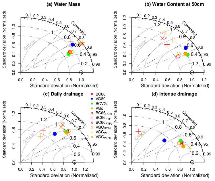
Figure 12 Taylor diagrams for hourly total water mass (a), hourly volumetric water content at 0.5 m depth (b), daily drainage water (c), and daily intense drainage water events (d). Model approach BC66 is plotted in red, VG80 in blue, BCVG in green, and VGc in orange. Additional model approaches with a homogeneous soil profile (BCVG_HOM and VGc_HOM) are represented as open circles, with parameters estimated from the usual PTFs (BCVG_PTF and VGc_PTF) by pluses (+) and with parameters estimated with PTFs, except or b (BCVG${}_{{\mathrm{PTF}}_b}$) or n (VGc${}_{{\mathrm{PTF}}_n}$), which are estimated in situ, by crosses (×). The Pearson correlation coefficient, the centred root mean square error (CRMSE), and the normalized standard deviation are summarized in this diagram (Taylor, 2001).

For the water mass and volumetric water content (Fig. 12a and b), scores are calculated at an hourly time step, while a daily time step is used for the drainage water over both the full period and the 110 intense drainage water events (Fig. 12c and d). BC66, BCVG, and VGc obtain good results, especially for predicting water mass, volumetric water content, and drainage water during intense events. Consistent with the previous results, VG80 obtains significantly lower scores, whatever the observable. VGc exhibits a larger score in terms of the intense drainage events and the same scores as BC66 and BCVG for other variables. These results highlight that the VGc model of Iden et al. (2015) is a very interesting alternative to the VG80 model for hydrological applications with an LSM, while maintaining an approach that is integrally based on closed‐form equations from van Genuchten (1980).

5 Sensitivity model approaches

5.1 Homogeneous soil profile

As LSMs are used on regional to global scales, their soil parameters are usually derived from soil maps that generally consider a homogeneous soil profile. To evaluate the influence of the variation in the depth of soil hydrodynamic parameters on our simulations, we performed a sensitivity test with a uniform soil profile using the BC66 model (BC66_HOM) and the VGc model (VGc_HOM). This uniform profile is fed with the vertical mean value of each parameter for each lysimeter (crosses in Fig. 3). Using a homogeneous profile in BC66_HOM and VGc_HOM significantly degrades the scores in terms of the water content (Fig. 12) but has a limited impact on the simulated water budget compared to BC66 and VGc (Fig. 9). It has a stronger impact on intense drainage events than on the whole time series (Fig. 12 and Table 2). Figure 13 shows very clearly that BC66_HOM fails to capture the observed soil moisture profile (drier surface conditions and wetter with depth), which is in contrast with BC66 (Figs. 10 and 11). VGc_HOM exhibits the same behaviour (Fig. S5). The drainage water dynamics are less impacted during winter than during spring, as shown by the BC66_HOM NASH scores, compared to BC66 (and accordingly for VGc_HOM and VGc). Indeed, lysimeter soils simulated with a homogeneous profile appear wetter than the observations and reference simulations, especially in spring. This wetter state thus induces the reactivity of the drainage water during this period that is too intense, thereby reducing the simulated skill scores compared to the reference simulations. This fact underlines that using a homogeneous soil profile sometimes fails to correctly simulate the drainage dynamic in the studied lysimeters for some conditions.

Figure 13 Same as Figs. 10 and 11 but for sensitivity model approaches with a homogeneous soil profile (BC66_HOM), with soil parameters from the usual PTFs (BC66_PTF), and with parameters from the usual PTFs, except for b, estimated in situ (BC66${}_{{\mathrm{PTF}}_b}$).

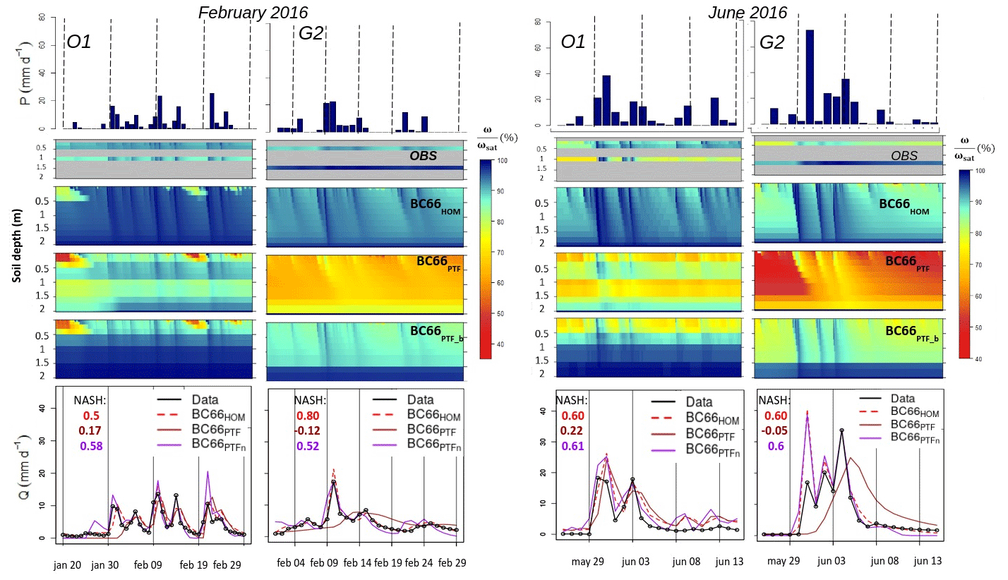
Table 2 NASH scores for the simulated drainage water (Q_drain) over the seven lysimeters and the entire period and during intense drainage water events (Q_int). Model approaches are shown with the soil hydrodynamic parameters set, with a homogeneous vertical profile (BC66_HOM and VGc_HOM), computed using the usual PTFs (BC66_PTF and VGc_PTF), or derived from observations (BC66 and VGc). The NASH of the additional model approaches with one parameter (n, ψ_sat, ω_sat, or k_sat) that keeps the reference values is also given.

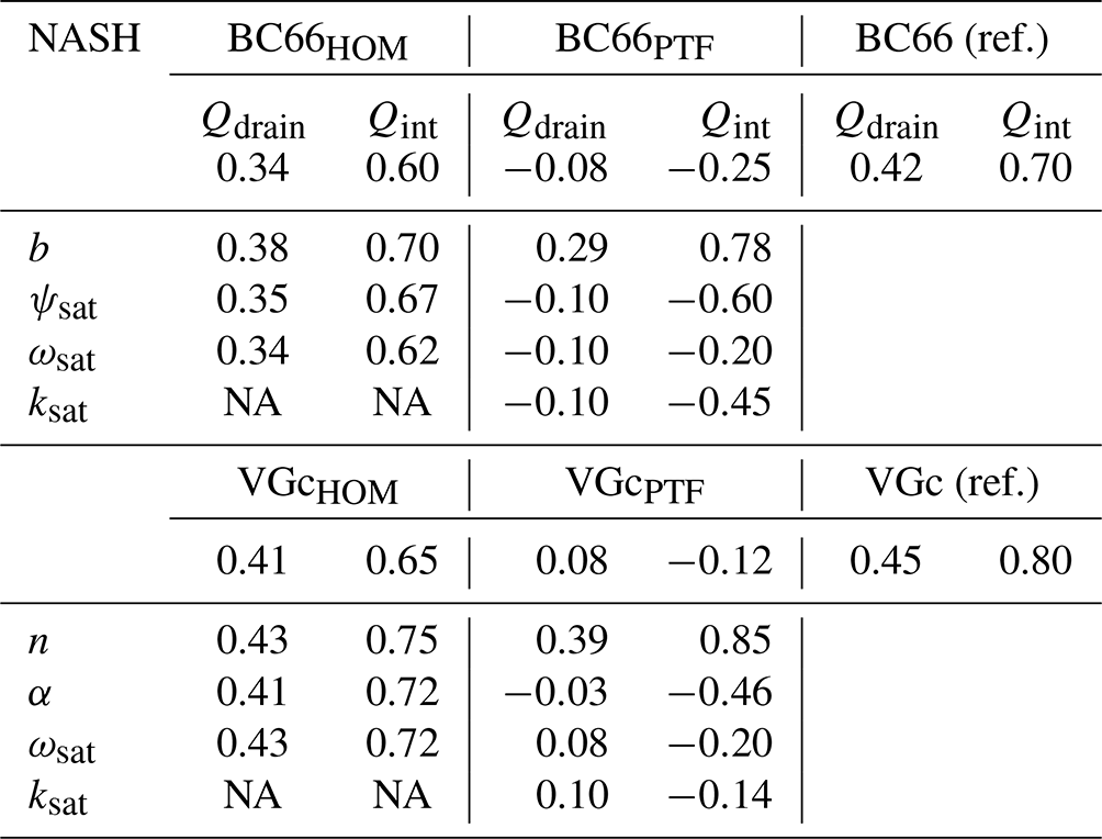
NA: not available

In order to determine which hydrodynamical parameter (via its vertical profile) has the largest impact on the simulations, we performed additional sensitivity tests with homogeneous soil profiles for all parameters, except for one that keeps its estimated heterogeneous profile. These tests are performed with all parameters being homogeneous, except one, with either ω_sat, b, or ψ_sat for BC66 and ω_sat, n, or α for VGc.

Using the seven lysimeters, we are able to complete the drainage water time series and all the selected intense drainage water events, as in Sect. 4.4. Table 2 shows that b and n are the most important parameters, as accounting for their heterogeneous profiles improves the NASH score more, compared to the other parameters. Their NASH scores are, in addition, very close to the BC66 and VGc references. These tests demonstrate the importance of b (and therefore n) for accurately simulating the drainage water dynamic and intense drainage water events. This finding is in agreement with previous studies (Ritter et al., 2003) that demonstrated a strong sensitivity of the simulated drainage water to n (and therefore b) and a lower sensitivity to k_sat.

5.2 Usual pedotransfer functions

LSMs commonly use PTFs to derive soil hydrodynamic parameters from soil textural information. As shown in Fig. 3, the soil parameters estimated from our measurements can be very different from those derived from six usual PTFs (Clapp and Hornberger, 1978; Cosby et al., 1984; Carsel and Parrish, 1988; Wösten and van Genuchten, 1988; Vereecken et al., 1989; Weynants et al., 2009). This is especially true for the b and n parameters. To investigate the impacts of such differences, sensitivity tests noted that BC66_PTF and VGc_PTF are performed so that the soil hydrodynamic parameters in each soil horizon are derived from the mean of these PTFs. Impacts on the simulated water budget are clear but not obvious enough to comment on (Fig. 9), even if BC66_PTF and VGc_PTF tend to increase the drainage water at the expense of evapotranspiration compared to BC66 and VGc in the GISFI lysimeters, while the opposite behaviour (lower drainage water and larger evapotranspiration) is found for the OPE lysimeters. All skill scores are drastically degraded in terms of water mass variations, volumetric water content at 0.5 m depth, daily drainage water, and intense drainage events (Fig. 12 and Table 2). These weaknesses are highlighted over the selected February and June 2016 events (Figs. 13 and S5). The soil water profile simulated by BC66_PTF and VGc_PTF is strongly underestimated compared to the observations, especially for the G2 lysimeter. This weakness induces a significant delay in the simulated drainage water, compared to observations and to other simulations.

Once again, the b and n parameters seem to be the key to this weakness. Indeed, we performed a set of tests using the BC66_PTF and VGc_PTF configuration, except for one parameter, either b (or n), ω_sat, ψ_sat (or α), or k_sat, that keeps its estimated in situ value. The use of the in situ estimated values of b and n tends to balance the water budget toward its partitioning of the reference (Fig. 9), especially with VGc. It drastically improves all skill scores compared to BC66_PTF and VGc_PTF (Fig. 12). This is also the case for the simulation of the soil water profile and especially the soil drainage water dynamic (Table 2; Figs. 13 and S5).

5.3 Lower boundary conditions

LSMs commonly use free-drainage lower boundary conditions (LBCs) on field sites or in regional- and global-scale application. We wondered if such an LBC is able to impact our results, compared to the seepage face LBC classically used to simulate lysimeters. Four simulations were performed using the same four model approaches as previously but with a free-drainage LBC instead of a seepage face LBC.

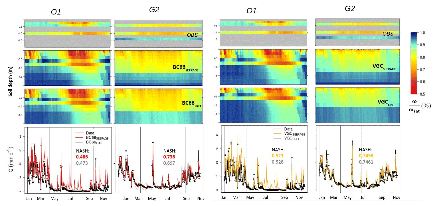
Figure 14 Mean annual cycles of the hourly effective wetting saturation profile (%) and daily drainage water (mm d⁻¹) observed (OBS in black) and simulated by BC66 (left panels) and VGc (right panels), with a seepage face LBC (BC66_SEEPAGE in red and VGc_SEEPAGE in orange) and a free-drainage LBC (BC66_FREE and VGc_FREE in grey) over lysimeters O1 and G2. The NASH scores for each simulated drainage water are also given.

Figure 14 shows the mean daily annual cycles of the soil moisture profiles and the drainage water observed and simulated by BC66 and VGc, with the two LBC approaches (BC66_FREE and VGc_FREE compared to BC66_SEEPAGE and VGc_SEEPAGE) for the O1 and G2 lysimeters. Soil moisture profiles are sensibly the same, even if, logically, the deep layers are slightly drier because the deepest layer is always saturated with a seepage face LBC. This fact is confirmed for all model approaches (BC66, VG80, BCVG, and VGc) which exhibit the same skill score in terms of water mass variations and volumetric water content at 0.5 m, whatever the LBC (comparing Figs. 12 and S6). The simulated total water budgets are also relatively unchanged (Fig. S7).

In terms of the daily drainage, the simulated response is not very different, whatever the LBC (Fig. 14). To use a seepage face LBC seems effectively more adequate for simulating drainage water in our lysimeters during recession periods, especially with BC66 (that explains the larger NASH for BC66_SEEPAGE compared to BC66_FREE for the G2 lysimeter). Some peaks of drainage water are also more pronounced with such an LBC. Comparing the Taylor diagrams (Figs. 12 and S6) underlines that all model approaches (BC66, VG80, BCVG, and VGc) reproduce daily drainage water and intense drainage events with the same accuracy, whatever the LBC.

6 Discussion and conclusion

This study uses time series (up to 7 years) from several lysimeters to evaluate the dynamics of water transfer in the unsaturated zone simulated with the land surface model ISBA. These observations allow the derivation of the heterogeneous profile of soil parameters. Although the original version of ISBA performed well, a set of four water closure relationships, which estimate the evolution of soil hydrodynamic properties with soil moisture, are tested. A comparison of these four relationships shows that, when soil parameters and meteorologic forcing are known, ISBA reproduces the evolution of soil hydrology and vegetation processes reasonably well. The choice to use a seepage face LBC in ISBA (as commonly done to simulate lysimeters) instead of its usual free-drainage LBC has a very little impact on the results.

The simulation using the VG80 water closure relationships exhibits more difficulty when reproducing the soil water profile and the drainage water dynamic, in particular during intense drainage water events, than the original ISBA version using the BC66 equations. This is partly linked to the limitation of the VG80 hydraulic conductivity function for n close to 1. The BCVG model approach combines the soil matrix potential function from VG80 with the hydraulic conductivity function from BC66, and the VGc model approach of Iden et al. (2015) that includes a maximum pore radius on the VG80 hydraulic conductivity curve solves these problems and even seems to be able to improve the simulation of the soil drainage water dynamic compared to BC66. However, the l parameter in the VG80 hydraulic conductivity (Eq. 3), and thus VGc (Eq. 5), is difficult to set, even with direct observations. In our study, it is fixed at the classical 0.5 value for some lysimeters but can vary drastically in others, which is consistent with the literature (Wösten and van Genuchten, 1988; Wösten et al., 2001; Schaap et al., 2001), underlying the difficulty with respect to estimating this parameter for regional- to global-scale applications.

The observations show that the soil hydrodynamic parameters in each lysimeter are strongly heterogeneous with depth, while LSMs generally use homogeneous profiles. Using additional sensitivity tests with such homogeneous profiles, we found that, even if the simulated soil water and drainage water dynamics remain acceptable compared to the observations, then all of the skill scores are worsened (especially for the soil water profile) compared to the model approaches with a heterogeneous profile. This finding supports the need to account for the vertical heterogeneity of soil hydrodynamic parameters (King et al., 1999; Mirus, 2015; Hengl et al., 2017; Vogel, 2019; Fatichi et al., 2020; Bauser et al., 2020; Gebler et al., 2017) to improve the simulation of soil water and drainage water dynamics (Stieglitz et al., 1997; Mohanty and Zhu, 2007; Decharme et al., 2011; Vereecken et al., 2019). This is a challenge for simulating groundwater recharge on regional and global scales.

We also found that parameters b and n, which characterize the shape of the soil water retention function, derived from the observations differ significantly from those derived from PTFs commonly used in LSMs (Clapp and Hornberger, 1978; Cosby et al., 1984; Carsel and Parrish, 1988; Wösten and van Genuchten, 1988; Vereecken et al., 1989; Weynants et al., 2009). Sensitivity tests show that the values of b and n derived from usual PTFs are not suitable for simulating the drainage water dynamic, at least for the seven lysimeters used in this study. In addition, these parameters exhibit the largest heterogeneity with soil depth. Neglecting this behaviour contributes to degrading the simulated drainage water dynamic. Note that this heterogeneous behaviour of b and n is still under consideration in the literature. As in our study, some authors observed a decrease in n with soil depth (Ritter et al., 2003; Jhorar et al., 2004; Schwärzel et al., 2006), while some others showed an increase (Groh et al., 2018) or even no change (Schneider et al., 2021). In any case, b and n could be the key parameters for correctly simulating the drainage water dynamic and groundwater recharge with LSMs. We recognize that this last assumption has to be confirmed in many other experimental field sites. Indeed, this study is based on two experimental sites with similar climatic conditions and with low-intensity precipitation events compared to other regions. It would be interesting to conduct additional studies in other contrasting climates.

In the context of LSMs that can be used at the regional or global scale, the major challenge is to simplify the numerical simulations and parameter calibration to be applicable in different contexts, without specific calibration, and to reproduce the water cycle as much as possible. This study at the local scale increases the confidence that LSMs are powerful tools for simulating the recharge of groundwater in different environmental conditions, with many soils and vegetation cover types, and can therefore be used for many applications in hydrology at both the regional and global scales. The sensitivity of our LSM to the soil heterogeneity or the value of some hydrodynamical parameters underlines, however, that this remains a challenge, even with the advent of global databases describing the vertical profile of the soil properties at depths greater than 1 m (Poggio et al., 2021).

Appendix A: Statistical scores

In this study, we used the following skill scores considering the simulated, S_i, and the observed, O_i, data defined at N discrete points in time, including:

• the overall bias,

  $$\begin{array}{}\text{(A1)}& \mathrm{Bias}=\stackrel{\mathrm{‾}}{S}-\stackrel{\mathrm{‾}}{O}\mathrm{with}\stackrel{\mathrm{‾}}{S}={\displaystyle \frac{\mathrm{1}}{N}}\sum _{i=\mathrm{1}}^N{S}_i\mathrm{and}\stackrel{\mathrm{‾}}{O}={\displaystyle \frac{\mathrm{1}}{N}}\sum _{i=\mathrm{1}}^N{O}_i;\end{array}$$

• the centred root mean square error,

  $$\begin{array}{}\text{(A2)}& \mathrm{CRMSE}=\sqrt{{\displaystyle \frac{\mathrm{1}}{N}}\sum _{i=\mathrm{1}}^N{\left[\left(S_i-\stackrel{\mathrm{‾}}{S}\right)-\left(O_i-\stackrel{\mathrm{‾}}{O}\right)\right]}^{\mathrm{2}}};\end{array}$$

• the Pearson correlation coefficient (or the coefficient of determination),

  $$\begin{array}{}\text{(A3)}& R={\displaystyle \frac{\frac{\mathrm{1}}{N}\sum _{i=\mathrm{1}}^N\left[\left(S_i-\stackrel{\mathrm{‾}}{S}\right)-\left(O_i-\stackrel{\mathrm{‾}}{O}\right)\right]}{{\mathit{\sigma }}_s{\mathit{\sigma }}_o}},\end{array}$$

  where σ_s and σ_o are the standard deviations of S_i and O_i, respectively. The coefficient of determination, R², is the square of the Pearson correlation; and

• the Nash and Sutcliffe (1970) efficiency criterion,

  $$\begin{array}{}\text{(A4)}& \mathrm{NASH}=\mathrm{1}-{\displaystyle \frac{\sum _{i=\mathrm{1}}^N{\left(S_i-O_i\right)}^{\mathrm{2}}}{\sum _{i=\mathrm{1}}^N{\left(O_i-\stackrel{\mathrm{‾}}{O}\right)}^{\mathrm{2}}}}.\end{array}$$