A gridded multi-site precipitation generator for complex terrain: an evaluation in the Austrian Alps

For climate change impact assessment, many applications require very high-resolution, spatiotemporally consistent precipitation data on current or future climate. In this regard, stochastic weather generators are designed as a statistical downscaling tool that can provide such data. Here, we adopt the precipitation generator framework of Kleiber et al. (2012), which is based on latent and transformed Gaussian processes, and propose an extension of that framework for a mountainous region with complex topography by allowing elevation dependence in the model. The model is used to generate two-dimensional fields of precipitation with a 1 km spatial resolution and a daily temporal resolution in a small region with highly complex terrain in the Austrian Alps. This study aims to evaluate the model with respect to its ability to simulate realistic precipitation fields over the region using historical observations from a network of 29 meteorological stations as input. The model's added value over the original setup and its limitations are also discussed. The results show that the model generates realistic fields of precipitation with good spatial and temporal variability. The model is able to generate some of the difficult areal statistics useful for impact assessment, such as the areal dry and wet spells of different lengths and the areal monthly mean of precipitation, with great accuracy. The model also captures the inter-seasonal and intra-seasonal variability very well, while the inter-annual variability is well captured in summer but largely underestimated in autumn and winter. The proposed model adds substantial value over the original modeling framework, specifically with respect to the precipitation amount. The model is unable to reproduce the realistic spatiotemporal characteristics of precipitation in autumn. We conclude that, with further development, the model is a promising tool for downscaling precipitation in complex terrain for a wide range of applications in impact assessment studies.

1 Introduction

Precipitation is a major component of the hydrological cycle. With global warming, the hydrological cycle is expected to intensify, and the risk associated with extreme events will increase (Tabari, 2020; Pfahl et al., 2017). The resulting changes in precipitation will be unequally distributed around the world. There are many hydrologic responses to climate change, and the potential impacts of these are likely to affect the availability of fresh water, agriculture, the timing and severity of wildfires, and habitat sustainability (Bates et al., 2008; Kundzewicz et al., 2008). With the increasing awareness of climate change and its global impacts on ecosystems and human societies (Konapala et al., 2020; Haddeland et al., 2014; Schewe et al., 2014), there is also an increasing need to understand the effects and impacts that would occur at the local scale. Knowledge of how the local hydrological cycle and water resources will be affected by climate change is essential for planning reliable adaptation strategies and water policy.

In Austria, where a large part of the country is covered by mountains, the local hydrological cycle depends heavily on temporal and spatial variations in precipitation. Tourism and agriculture are among the main drivers of Austria's economy, and the accessibility of water resources for human consumption and ecosystems is largely contingent on the spatiotemporal distribution of precipitation. In the Austrian Alps, studies on the observed and projected impact of climate change have shown changes in the availability of snow cover and water flux (e.g., Abermann et al., 2009; Wijngaard et al., 2016). This will ultimately have an impact on the economy, the ecosystem, the environment, and society. To assess the impacts of climate change at local scales, precise climate information is critical and can serve the requirements of decision-makers. Often, such information should be consistent in space and time for the present and future climate. Many applications in hydrology require very high-resolution precipitation data, typically at a 1 km spatial resolution and a daily temporal resolution. However, obtaining such high-resolution precipitation data is still a challenging task, especially in mountainous regions (Henn et al., 2018). Most importantly, for complex topography, such as the Austrian Alps, even a 1 km resolution cannot include the impact of topography on climate correctly. For such regions, many applications in hydrology and ecology require even higher-resolution data – at a spatial scale of 100 m and at an hourly temporal scale. Climate models with higher resolutions, like regional climate models, are also unable to provide such data. For this reason, various downscaling methods have been in use over the past few decades. Among these downscaling methods, statistical downscaling using stochastic weather generators (WGs) has become very popular, mainly because WGs are computationally parsimonious.

A vast variety of WGs have been developed based on different approaches. The most widely used WGs are founded on a rather simplistic approach in which the sites are mutually independent in space and time. Such WGs are generally referred to as “single-site” WGs. Among the single-site WGs, the most popular are the parametric models based on Richardson (1981). Richardson (1981) used a Markov chain to simulate time series of precipitation occurrence (wet/dry days) and amount, and other variables were generated upon the condition of whether the generated day was wet or dry (e.g., Dabhi et al., 2021; Caron et al., 2008; Zhang et al., 2004; Dubrovský et al., 2004; Wilks, 1992). Details on the available WGs can be found in the review articles by Ailliot et al. (2015), Maraun et al. (2010), and Wilks and Wilby (1999); Maraun et al. (2010) focused solely on precipitation.

The major drawback of single-site WGs is that they are only focused on a single location; this can generate realistic data at a location, but it lacks a spatially correlated structure in the generated data. Obtaining a spatially and temporally consistent dataset – which is more realistic – from single-site models is impossible. Thus, over the past 2 decades, the focus has moved towards the development of spatiotemporal WGs, also known as “multi-site” WGs. For precipitation with its uneven nature of occurrence and intensity, it is even more challenging to model it under the condition of maintaining its spatiotemporal structure. In particular, in complex topography, such as the Alps, this task is even more challenging.

Numerous approaches have been proposed to generate spatially and temporally correlated precipitation data. Wilks (1998) published one of the early works on the multi-site generation of daily precipitation data; in the aforementioned study, single-site parametric WGs at sites were forced with correlated random numbers to generate the occurrence of precipitation, and the amount of precipitation was generated using a mixture of two exponential distributions. Other approaches to the spatiotemporal modeling of precipitation are hidden Markov models (e.g., Ghamghami et al., 2016; Charles et al., 1999; Ailliot et al., 2009), copula-based approaches (Serinaldi, 2009; Bárdossy and Pegram, 2009), resampling based on the k-nearest-neighbors approach (Apipattanavis et al., 2007; Buishand and Brandsma, 2001; Rajagopalan and Lall, 1999), Poisson cluster models (Ramesh et al., 2012; Cowpertwait, 1995), artificial neural networks (Harpham and Wilby, 2005), and approaches based on generalized linear models (GLMs) (Kleiber et al., 2012; Verdin et al., 2018). Moreover, Baxevani and Lennartsson (2015) proposed a spatiotemporal model using a censored latent Gaussian field for precipitation generation, Olson and Kleiber (2017) used the approximate Bayesian computation method, and Gao et al. (2021) developed a multi-site stochastic daily rainfall model by coupling a univariate Markov chain with a multi-site rainfall event model. More sophisticated WGs also exist that can provide high-resolution spatiotemporal fields combining physical and stochastic approaches (e.g., Peleg et al., 2017; Paschalis et al., 2013).

However, most of the aforementioned approaches simulate precipitation only at the locations where observations are available, and such multi-site WGs have been implemented for the Alps; for example, Keller et al. (2015) and Keller et al. (2017) used a Wilks-type WG for precipitation simulation and downscaling, respectively, for a mountainous catchment in the Swiss Alps, and Breinl et al. (2013) used a semi-parametric multi-site precipitation generator for the mountains in the Austrian–German Alps. Nevertheless, high-resolution data in space and time are needed to provide more realistic input for local climate impact assessment. To achieve this, a gridded multi-site model is required. Sparks et al. (2017) proposed a multi-site multivariate WG based on the use of periodically extended empirical orthogonal functions (EOFs), in which they modeled precipitation as a censored latent Gaussian process. They generated gridded precipitation and temperature data over Europe using gridded input data, but their WG cannot provide gridded data without gridded observations. Peleg et al. (2017) developed a WG called AWE-GEN-2d, which can generate two-dimensional fields of various meteorological variables where precipitation is generated at a 2 km spatial resolution and a 5 min temporal resolution, and used it in the Swiss Alps. Although their approach is sophisticated, as it is a hybrid approach combining dynamical and statistical approaches, it requires spatially distributed data for the calibration of the WG and cannot generate data for a region outside of the calibration region. Such WGs are of limited use if the observed gridded data are not available, which is often the case. To our knowledge, not much work has been done on complex terrain, like the European Alps, using multi-site gridded WGs without gridded observations.

Wilks (2009) developed one of the first ever WGs that could provide gridded data of precipitation and temperature at locations with no observations. Kleiber et al. (2012) also provided an approach using a GLM-based model that utilizes Gaussian processes to generate gridded data. Their approach is appealing, as it generates the readily available field of precipitation using kriging for the interpolation of the model parameters. The advantage of their approach is that one could include various covariates in the GLM framework, such as large-scale climate indices, local climate information, and topographical information, which makes the model more flexible. Another advantage is that it is a probabilistic approach that allows one to quantify the uncertainties in the parameter estimation. However, Kleiber et al. (2012) only tested the model for multi-site precipitation generation, i.e., at locations with observation, and not for generated gridded data of precipitation. As many applications for impact studies require gridded data as input, prior to producing the gridded data for such applications, one must evaluate the model for its ability to reproduce gridded fields. Another important point to be noted is, as the model can provide data at locations without historical observations, one can obtain historical time series of daily precipitation at those locations. In order to use the model for this purpose, it is necessary to assess the model performance with respect to gridded fields. Verdin et al. (2018) modified the framework of Kleiber et al. (2012) by including seasonal precipitation as an additional covariate, and they evaluated the model for gridded data, although it was implemented on flat terrain. Moreover, their modified model and the original model both used an isotropic and stationary covariance structure with ordinary kriging (OK) for the interpolation of the model parameters; this may not be suitable for complex topographical terrain. Bennett et al. (2018) generated precipitation fields using a latent-variable approach that provides a parsimonious method to jointly generate the rainfall occurrence and amount. They used an isotropic, powered exponential function to include spatial correlations and kriging for the interpolation of the parameters. However, they also implemented their model in relatively flat terrain in South Australia. To our knowledge, no space–time gridded precipitation generator has been evaluated with respect to its ability to generate two-dimensional fields of precipitation in the highly complex terrain without the requirement for gridded input data.

Here, we propose an extension of the framework of Kleiber et al. (2012) for complex terrain and evaluate the model with respect to its capability to generate realistic two-dimensional fields of precipitation for a mountainous region in the Austrian Alps. In addition, we examine the added value of our model over the original isotropic setup and discuss the limitations of the model.

This article is organized as follows: Sect. 2 describes the extension of the isotropic framework for the implementation in a mountainous region; Sect. 3 details the study area, the data, and the model evaluation strategy used in the study; Sect. 4 presents and analyses the results; Sect. 5 comprises a discussion of the results; and Sect. 6 summarizes the study.

2 Model description

2.1 Precipitation occurrence

At a location s and on a day t, the precipitation occurrence O(s,t) is 0 (dry day) if no precipitation occurs and 1 (wet day) if precipitation occurs. A wet day is defined as a precipitation amount in excess of 0.1 mm.

For a set of locations s and on a day t, a latent Gaussian process W_O(s,t) is defined with a mean function μ_O(s,t) and a covariance function $C_{\mathrm{O}}(\mathit{h},\mathit{v},t)$, where $h=|s_i-s_j|$ is the horizontal (Euclidean) distance between two locations denoted by i and j and $v=|v_i-v_j|$ is the elevation difference between the two locations. The suffix “O” stands for occurrence. As we are implementing the model in a mountainous region, we also define the covariances among the sites as a function of the difference in the elevation. In comparison with the original model, where an isotropic covariance structure is used as a function of horizontal distances among the sites, this allows us to include anisotropy in the model. The precipitation occurrence then is defined as follows:

$$\begin{array}{}\text{(1)}& \begin{array}{r}O(\mathit{s},t)=\mathrm{0}\mathrm{if}{W}_{\mathrm{O}}(\mathit{s},t)<\mathrm{0},\\ O(\mathit{s},t)=\mathrm{1}\mathrm{if}{W}_{\mathrm{O}}(\mathit{s},t)\ge \mathrm{0}.\end{array}\end{array}$$

Here, the mean function is

$$\begin{array}{}\text{(2)}& {\mathit{\mu }}_{\mathrm{O}}(\mathit{s},t)={\mathit{\beta }}_{\mathrm{O}}^{\prime }\left(\mathit{s}\right){\mathit{X}}_{\mathrm{O}}(\mathit{s},t),\end{array}$$

where X_O is a vector of covariates and β_O is a vector of regression parameters, as in Eq. (5).

Kleiber et al. (2012) used a stationary and isotropic exponential covariance function of the form

$$\begin{array}{}\text{(3)}& C(\mathit{h},t)=\exp \left({\displaystyle \frac{-\left|\mathit{h}\right|}{A\left(t\right)}}\right),\end{array}$$

where A(t) is the time-dependent scale parameter.

As our goal is to use the model in complex topography, we introduce anisotropy in the covariance function (Eq. 3) by taking the difference in elevation between two locations. Thus, our stationary and anisotropic covariance function $C(\mathit{h},\mathit{v},t)$ takes the following form:

$$\begin{array}{}\text{(4)}& C_{\mathrm{O}}(\mathit{h},\mathit{v},t)=\exp \left(-{\displaystyle \frac{\left|\mathit{h}\right|}{A\left(t\right)}}-{\displaystyle \frac{\left|\mathit{v}\right|}{B\left(t\right)}}\right),\end{array}$$

where A(t) and B(t) are the time-dependent scale parameters in the horizontal and vertical directions, respectively.

Elevation dependence in the covariance structure is a natural assumption in complex terrain. In the literature (e.g., Wilks, 1999, 2009), it has been used for precipitation simulation in the mountains.

At the base of this model is the single-site precipitation generator based on a GLM framework (e.g., Stern and Coe, 1984; Chandler and Wheater, 2002; Furrer and Katz, 2007); this is similar to a Richardson-type precipitation generator (Richardson, 1981), in which the daily precipitation occurrence is modeled as a first-order Markov chain and the daily precipitation amount is modeled using a gamma distribution. The GLM-based approach allows more flexibility, as one may include as many covariates as desirable; therefore, the seasonality or the influence of large-scale circulation on the local precipitation can be included. In the GLM approach, taking the previous day's occurrence as a covariate forms a first-order Markov chain. Thus, at individual sites, the model reduces to a logit model given by

$$\begin{array}{}\text{(5)}& \log \left({\displaystyle \frac{p_t}{\mathrm{1}-p_t}}\right)={\mathit{\beta }}_{\mathrm{O}}^{\prime }\left(s\right){\mathit{X}}_{\mathrm{O}}(s,t),\end{array}$$

where p_t is the probability of occurrence on a day t.

Note that we use a logit link function instead of a probit link function, as was the choice in the original model. The parameters β_O are estimated at each location using the maximum likelihood estimation (MLE) approach.

In order to spatialize the model to obtain gridded data, the estimated regression parameters at observation locations must be interpolated at grid locations. The Gaussian process allows for a spatial interpolation method called kriging; this method allows one to interpolate the model parameters β_O associated with each covariate (estimated at the observation locations) to any location of interest. These interpolated coefficients are then used to obtain the mean function (Eq. 2). Here, we use kriging with external drift (KED) to interpolate the regression parameters. As precipitation in the mountains is unequally distributed across terrain, we allow elevation as an external drift in kriging such that the predicted values of precipitation (through the interpolated parameters) reflect the elevation dependence of precipitation. Again, inclusion of the elevation in kriging interpolation is natural in complex terrain. It has been used in the literature for precipitation interpolation in the mountains and proven to outperform OK (e.g., Tobin et al., 2011; Rata et al., 2020). Moreover, we have found linear dependence in the model parameters with elevation (not shown). In KED, an auxiliary variable is assumed (which is elevation here) that is linearly related to the variable of interest (which is the β parameter associated with each covariate in the model).

The variogram for the regression parameter associated with each of the covariates is estimated using the MLE. The nugget gets close to zero. Once the parameters of the logit model are interpolated, precipitation occurrence can be modeled at each grid point. However, the generated gridded field of precipitation occurrence, which is correlated in space, must also be correlated in time. Hence, the time-dependent covariance $C_{\mathrm{O}}(\mathit{h},\mathit{v},t)$ (see Eq. 4) has been introduced. This covariance is estimated using the residuals in the logit model. We use the method of moments approach, as suggested by Kleiber et al. (2012), to estimate the parameters of the covariance function. The parameters are estimated separately for each month to allow for seasonality in the generated data. Following this process, the generated field of precipitation occurrence is correlated in both space and time and also reflects the seasonality.

Note that Gaussian process modeling is considered a nonparametric method. In a parametric model, the number of parameters remains fixed with respect to the amount of data available (i.e., number of stations in our case), whereas the number of parameters grows with the number of data points when using nonparametric methods.

We also compare the results of our model with a simulation using ordinary kriging (OK) instead of KED in our model as well as with the original isotropic model using OK and KED. This will be discussed in Sect. 4.3.

2.2 Precipitation amount

To simulate spatially correlated fields of precipitation, another Gaussian process W_A(s,t) is defined with a mean function μ_A(s,t) and a covariance function $C_{\mathrm{A}}(\mathit{h},\mathit{v},t)$ such that

$$\begin{array}{}\text{(6)}& Y(\mathit{s},t)=G_{\mathit{s},t}^{-\mathrm{1}}\left(\mathrm{\Phi }\left(W_{\mathrm{A}}(\mathit{s},t)\right)\right).\end{array}$$

Here, G_s,t is the cumulative distribution function (CDF) of the gamma distribution at the location s and time t, and Φ is the CDF of a standard normal distribution. The suffix “A” stands for amount.

At an individual location, the amount model is the gamma GLM with a logarithmic link function as given by Furrer and Katz (2007). The shape parameter α of the gamma distribution varies in space but not in time, whereas the scale parameter γ varies in both space and time. Hence, each location has its own distinct value of shape and scale parameters, with the scale parameter varying with time. Thus, we have

$$\begin{array}{}\text{(7)}& \log \left(\mathit{\gamma }\right(\mathit{s},t\left)\mathit{\alpha }\right(\mathit{s}\left)\right)={\mathit{\beta }}_{\mathrm{A}}^{\prime }\left(\mathit{s}\right){\mathit{X}}_{\mathrm{A}}(\mathit{s},t),\end{array}$$

with the mean of the gamma distribution being the product of the scale and shape parameters, i.e., γα. X_A is the vector of covariates possibly different from those selected in the occurrence model.

The scale and shape parameters (γ and α, respectively) and the model parameters (β_A) are estimated at each individual observation site using the MLE approach and are then interpolated using KED. We allow the scale parameter to vary with every month in order to include seasonal variations in precipitation at each location.

The mean function μ_A(s,t) of the Gaussian process W_A(s,t) is again obtained from a regression on covariates. The covariance function $C_{\mathrm{A}}(\mathit{h},\mathit{v},t)$ is the same as that given in the occurrence model (Eq. 4) but with different parameters. The parameters of the covariance function are estimated for each month separately using the method of moments approach in order to allow seasonality in the spatiotemporal pattern of the precipitation amount.

3 Implementation

3.1 Study area and data

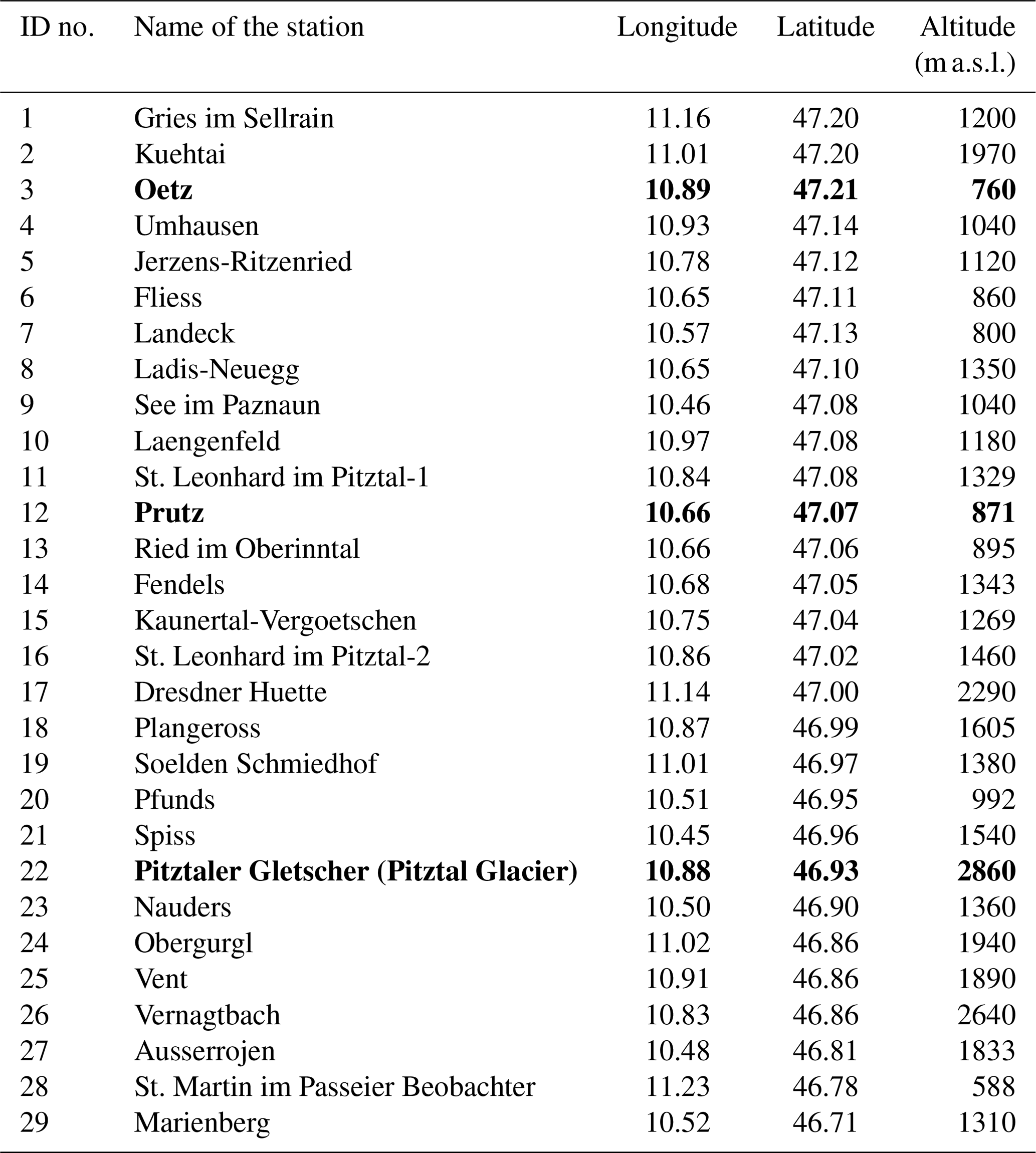
The model is implemented in a small region comprising highly complex terrain (ranging from 256 to over 3500 m a.s.l., meters above sea level) in the Austrian Alps. The area surrounds the catchment of the Oetz River, mainly in the federal state of Tyrol but also including a part of the Autonomous Province of Bolzano in northern Italy. The reason for selecting this region is that the catchment of the Oetz River is a widely researched area (e.g., Wijngaard et al., 2016; Abermann et al., 2009). To include more stations in the study, we allowed stations from the surrounding region, including northern Italy. The study region is comprised of several valleys including the Oetz and Pitz valleys in Austria and the Passeier Valley in South Tyrol. Daily observations from 29 meteorological stations (Fig. 1) based on the availability of homogeneous time series for a period of 30 years from 1981 to 2010 are selected. Typically, input data for hydrological applications are required on an hourly temporal scale for the spatial scale of the terrain considered; however, due to the fact that very few hourly datasets are available over climate timescales, we selected daily data for the study. The dataset comprises data provided by the Austrian National Weather Service (ZAMG – Zentralanstalt für Meteorologie und Geodynamik), the Hydrographic Service of Austria, the Hydrographic Service of the Autonomous Province of Bolzano, the Institute of Atmospheric and Cryospheric Sciences – University of Innsbruck, and TIWAG (Tiroler Wasserkraft AG). The highest station is on a glacier (Hintereisferner) at an elevation of 2860 m a.s.l., whereas the lowest station is at 588 m a.s.l. in northern Italy. A few stations have missing values for single days or for a short period. Our model ignores such values while computing the observed statistics. The data at all of the stations are thoroughly quality controlled by the respective service providers.

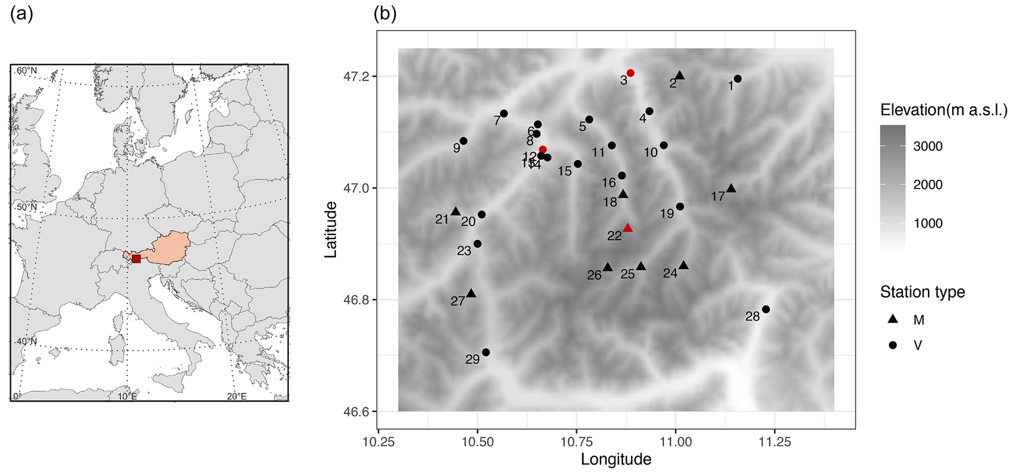
Figure 1 The study area used in this work showing (a) the location of the region in the central Alps and (b) the locations of the 29 meteorological observation stations whose data are used in the study. Latitude and longitude are given in degrees north and east, respectively. Gray shading denotes the elevation (m a.s.l.). Stations with an elevation higher than 1500 m a.s.l., usually high-mountain stations, are shown using the symbol “M”, and the stations with an elevation lower than 1500 m a.s.l., typically the valley stations, are shown using the symbol “V”. The stations shown in red are selected as example stations to illustrate the results in the article.

In the northern part of the region, we have a dense network of stations, whereas the southern part has relatively fewer stations. The average inter-station distance between two locations is 28.15 km, the maximum inter-station distance is 72.84 km, and the minimum inter-station distance is 1.25 km. The average altitude difference between two stations is 0.605 km, while the maximum altitude difference is 2.272 km. The locations of the 29 stations are shown in Fig. 1, and further details about the stations are given in Table 1.

Table 1 List of the 29 meteorological stations whose data are used in the study. The names in bold are the three representative stations used to illustrate the results.

The mean annual precipitation observed in the lowlands is approximately 780 mm over an average of 150 wet days per year, whereas the highest mean annual precipitation of 1320 mm over an average of 176 wet days per year is observed at the high-mountain station of Dresdner Huette. The highest number of mean annual wet days is 220 at St. Martin in the Passeier Valley in South Tyrol, with an annual average of 887 mm of precipitation.

Due to strongly different topography, a large variability in both space and time is observed in the dataset. Of the 29 stations, Prutz has the most distinct climatological characteristics. For example, Prutz has the largest variability in almost all months. Moreover, the most extreme precipitation (156.5 mm) in a day is recorded at Prutz (in July 2009), while the second highest amount of precipitation amongst the remaining 28 stations was recorded on the same day at Dresdner Huette (35.1 mm). Apart from Prutz, only Dresdner Huette recorded a daily precipitation amount as high as 120.4 mm during the 30 years of record. At the St. Leonhard im Pitztal location, there are two stations operated by two different service providers: one by the Austrian Hydrographic Service (St. Leonhard im Pitztal-1; see Table 1) in the northern part of the valley and the other by ZAMG (St. Leonhard im Pitztal-2; see Table 1) in the southern part of the Pitz Valley. St. Leonhard im Pitztal-2 has somewhat different climatological characteristics than the nearby stations. Another station that has quite a different climatology compared with the Austrian stations is St. Martin. Note that this station is in the south of the Alpine crest (i.e., in northern Italy) and has the lowest elevation in the observed data. Thus, there are high variations in the observed climatologies of precipitation from valley to valley and also for stations within the same valley. This creates a particular challenge with respect to the simulation.

To reduce the sampling uncertainty and increase the robustness of the observations, we increase the sample size of the observed data by considering a 7 d window centered on the day of interest. Thus, the chance that a particular date had, for example, 30 dry days by random choice is minimized, thereby avoiding the probability of a dry day being 1.0 (rather than a value such as 0.98), which is a problematic model setting.

We generate N=30 stochastic realizations, each 30 years long (30 realizations × 30 years = 900 years), of daily two-dimensional fields of precipitation on a 1 km grid over the region using the aforementioned observed 30 years of daily data. The Shuttle Radar Topography Mission (SRTM) 1 km (30 arcsec) resolution dataset (Becker et al., 2009) is used as a simulation grid. We select a 1 km spatial resolution to reduce the simulation time and the data storage requirements.

For the Northern Atlantic Oscillation Index (NAOI) (see Sect. 3.2), a daily time series from 1981 to 2010 is obtained from the National Oceanic and Atmospheric Administration (NOAA) website (https://www.cpc.ncep.noaa.gov/products/precip/CWlink/pna/nao.shtml, last access: 15 May 2023).

Note that the observed data are from different service providers; therefore, the time of the data collection may differ, which may affect the results.

3.2 The selection of covariates in the model

We allow several covariates in the model so that the model can capture a realistic structure of precipitation patterns over the region. This includes the day-to-day time dependence, the seasonality, and the influence of large-scale circulation. As the first covariate, we select the occurrence of precipitation on the day prior (Occ_t−1) as a possible covariate so that day-to-day temporal dependency in occurrence at a location is captured. To include seasonality, the time-dependent first- and second-order harmonics of sine and cosine (see Table 2) are considered as possible covariates. To allow for the influence of large-scale circulation over Europe, the NAOI is considered as a possible covariate. Studies show that there are links between the NAOI and precipitation characteristics (Casty et al., 2005; Beniston, 1997). A strongly positive NAOI is associated with persistent high pressure over the Alpine region, resulting in warmer than average temperatures and lower than average precipitation. In general, the winter NAOI correlates negatively with precipitation. Along with the described covariates, we also consider their interaction terms as possible covariates.

Table 2 List of the covariates included in the occurrence and amount models (Eqs. 8 and 9, respectively).

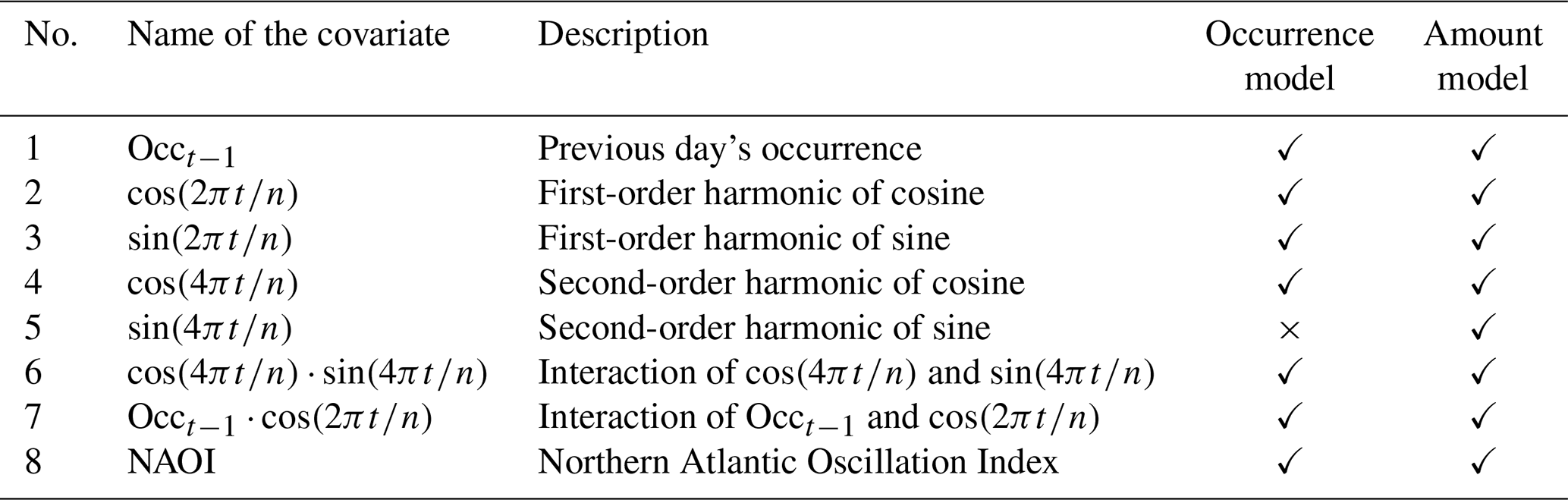
“n” is 365 (366 in the case of a leap year).

For the selection of the covariates in the model, we use both the Akaike information criterion (AIC) (Akaike, 1974) and the Bayesian information criterion (BIC) (Schwarz, 1978). The criteria do not select the same set of covariates at all of the stations: the BIC has a tendency to select the simplest model, whereas the AIC has a tendency to select more complex models. However, it turns out that the BIC helps to identify the most important covariates at all of the stations.

The three most important covariates for the occurrence model at the majority of stations are Occ_t−1, $\cos (\mathrm{2}\mathit{\pi }t/n)$, and $\cos (\mathrm{4}\mathit{\pi }t/n)$, where “t” is the day of the year. We select the covariates that are selected by both the AIC and BIC at the majority stations. The selected covariates are listed in Table 2. The BIC selected this set of covariates at 18 of the 29 stations (see Sect. 3.1), whereas the AIC selected the same set of covariates at 11 stations. Thus, the vector of covariates in the model is as follows:

$$\begin{array}{}\text{(8)}& \begin{array}{rl}{\mathit{X}}_{\mathrm{O}}(s,t)=& \left(\mathrm{1},{\mathrm{Occ}}_{t-\mathrm{1}},\cos \left({\displaystyle \frac{\mathrm{2}\mathit{\pi }t}{n}}\right),\sin \left({\displaystyle \frac{\mathrm{2}\mathit{\pi }t}{n}}\right),\right.\\ & \cos \left({\displaystyle \frac{\mathrm{4}\mathit{\pi }t}{n}}\right),\cos \left({\displaystyle \frac{\mathrm{4}\mathit{\pi }t}{n}}\right)\cdot \sin \left({\displaystyle \frac{\mathrm{4}\mathit{\pi }t}{n}}\right),\\ & \left.{\mathrm{Occ}}_{t-\mathrm{1}}\cdot \cos \left({\displaystyle \frac{\mathrm{2}\mathit{\pi }t}{n}}\right),\mathrm{NAOI}\right),\end{array}\end{array}$$

where “n” is 365 (or 366 in the case of a leap year). The first term is associated with the intercept in the model.

For the precipitation amount, we also consider all of the possible covariates described for the occurrence model. Furthermore, as above, we select the covariates using both the AIC and BIC for the amount model. Additionally, selecting the same seven covariates as in the occurrence model at the majority of stations, the second-order harmonic of sine is also selected by both the AIC and BIC (17 stations by the BIC and 16 stations by the AIC). Thus, we allow a total of eight covariates in the amount model (see Table 2), and the vector of covariates for the amount model is as follows:

$$\begin{array}{}\text{(9)}& \begin{array}{rl}{\mathit{X}}_{\mathrm{A}}(s,t)=& \left(\mathrm{1},{\mathrm{Occ}}_{t-\mathrm{1}},\cos \left({\displaystyle \frac{\mathrm{2}\mathit{\pi }t}{n}}\right),\sin \left({\displaystyle \frac{\mathrm{2}\mathit{\pi }t}{n}}\right),\right.\\ & \cos \left({\displaystyle \frac{\mathrm{4}\mathit{\pi }t}{n}}\right),\sin \left({\displaystyle \frac{\mathrm{4}\mathit{\pi }t}{n}}\right),\cos \left({\displaystyle \frac{\mathrm{4}\mathit{\pi }t}{n}}\right)\\ & \left.\cdot \sin \left({\displaystyle \frac{\mathrm{4}\mathit{\pi }t}{n}}\right),{\mathrm{Occ}}_{t-\mathrm{1}}\cdot \cos \left({\displaystyle \frac{\mathrm{2}\mathit{\pi }t}{n}}\right),\mathrm{NAOI}\right).\end{array}\end{array}$$

The correlations for the precipitation amount in the model are computed only for days when precipitation was observed.

3.3 Model evaluation strategy

Although the model produces daily fields of precipitation, before evaluating the model for gridded data, we first evaluate it at the individual locations for which observations are available. It is common practice for the validation of WGs that first the input statistics must be reproduced. From the simulated gridded data, the 30-year time series of daily precipitation at the nearest grid point to the observation locations is extracted from each of the N=30 realizations. The mean of the simulated statistics in each realization is compared with the observed statistics. The validation is carried out for daily and long-term statistics, and more difficult statistics to be reproduced by the model are also considered. For the illustration of the results at individual locations, 3 example stations (from the 29 available stations) are selected: (i) Oetz, (ii) Pitztal Glacier, and (iii) Prutz. These three stations are highlighted in red in Fig. 1b. The three stations are selected such that Oetz represents the results at valley stations, Pitztal Glacier represents the results at high-mountain stations, and Prutz represents stations with different climatic characteristics and also has the climatic characteristics most distinct from those at the surrounding stations (which makes it the most challenging to simulate). Note that Pitztal Glacier is the highest station amongst the 29 observation stations (see Table 1).

In the next step, we evaluate the model with respect to its ability to reproduce spatial statistics. Thus, gridded observed data are required. We use the Alpine Precipitation Grid Dataset (APGD) (Isotta et al., 2014) from the Swiss Federal Office for Meteorology and Climatology (MeteoSwiss), which has a 5 km spatial resolution and a daily temporal resolution. The dataset is based on measurements from high-resolution rain gauge networks, incorporating more than 5500 rain gauge measurements on average per day from more than 8500 stations in seven Alpine countries. With a 10–15 km station spacing, the dataset is one of the densest in situ observation networks over high-Alpine topography worldwide. These data are available from 1971 to 2008. Note that this dataset is not a perfect reference. To obtain 30 years of gridded observations, we select the period from 1979 to 2008 for the validation of the simulated gridded data.

In order to assess the interpolation accuracy, we perform a holdout cross-validation in which one or more stations are withheld from the model fitting process. We withhold the same three stations that were selected for the illustration of the results: Oetz, Pitztal Glacier, and Prutz. The model should be able to reproduce the observed statistics accurately at the withheld stations. For cross-validation, we also generate N=30 realizations of 30 years, i.e., 900 years of data.

For the uncertainty estimation in the N=30 realizations, we use a tolerance interval (TI) (Patel, 1986; Krishnamoorthy and Mathew, 2009; Young, 2010) instead of the conventional method of using a confidence interval for the sampling error, which is sensitive to sample size. As opposed to confidence intervals, which would give expected bounds on the means of the simulated data, the TI gives bounds on the future individual observations. In our view, TIs provide an appropriate visualization of the expected variability in the simulated data as well as a means of comparison with the original data. Here, we use a parametric two-sided TI with a normal distribution. The TIs are computed for each of the statistics considered in this study, obtained from the simulated 30 realizations at each station. As uncertainty criteria, we select a confidence interval of 95 % and a 99 % proportion of the population for the TI, i.e., the TIs indicate the 99 % range of the simulated values (with 95 % confidence). The TIs are shown in each figure as a shaded area around the curve and are denoted as ${\mathrm{TI}}_{\mathrm{99}}^{\mathrm{95}}$ throughout the article.

To quantify the model performance, along with various error metrics, we also take correlation coefficients (CCs) and coefficients of determination (R² values) into account. Thus, we employ the following metrics: (i) mean bias error (MBE), (ii) mean absolute error (MAE), (iii) root-mean-square error (RMSE), (iv) CC, and (v) R². Each of the performance metrics serves a different purpose. The MBE measures the overall bias in the model performance, whereas the MAE and RMSE both provide information on the mean magnitude of the error, regardless of the direction of the error. However, the greater the difference between them, the greater the variance in the individual errors in the sample. Similarly, correlation shows the association between the two variables (which are the observed and synthetic statistics here), but R² shows the proportion of data variation explained by the model. All of the performance metrics for the spatial statistics (corresponding to Fig. 13) are obtained between the observed and synthetic statistics derived at all of the grid points; for example, for the spatial occurrence probabilities, the metrics are derived between the observed and synthetic “spatial series” of the occurrence probabilities.

4 Results

An extensive evaluation of the model-generated data is carried out here.

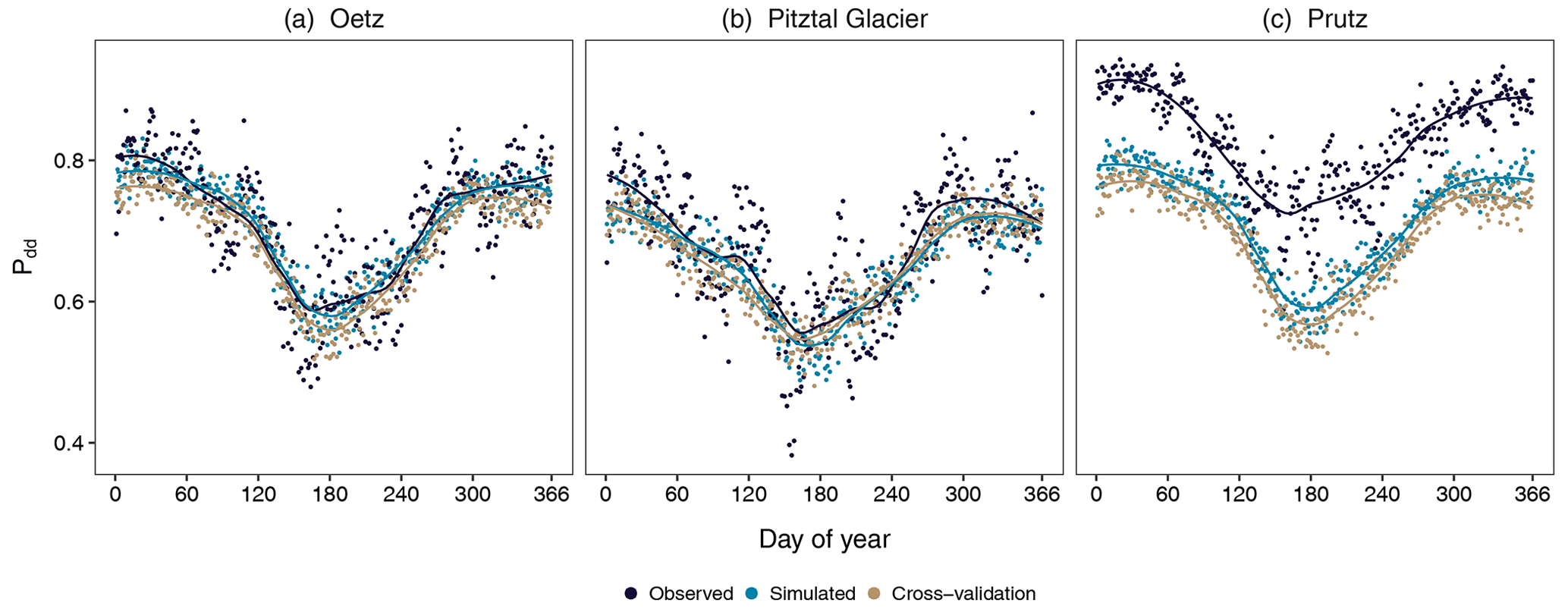
Figure 2 Daily conditional probability of a dry day following a dry day (P_dd) at three selected stations: (a) Oetz, (b) Pitztal Glacier, and (c) Prutz (Fig. 1, Table 1). The observed probabilities (navy blue) are obtained from the 30 years (1981–2010) of observed data. The simulated probabilities are the mean of the 30 realizations (sky blue) and of the holdout cross-validation simulation (brown). The solid lines are the curves fitted (using the LOESS method) to the observed and simulated probabilities, respectively.

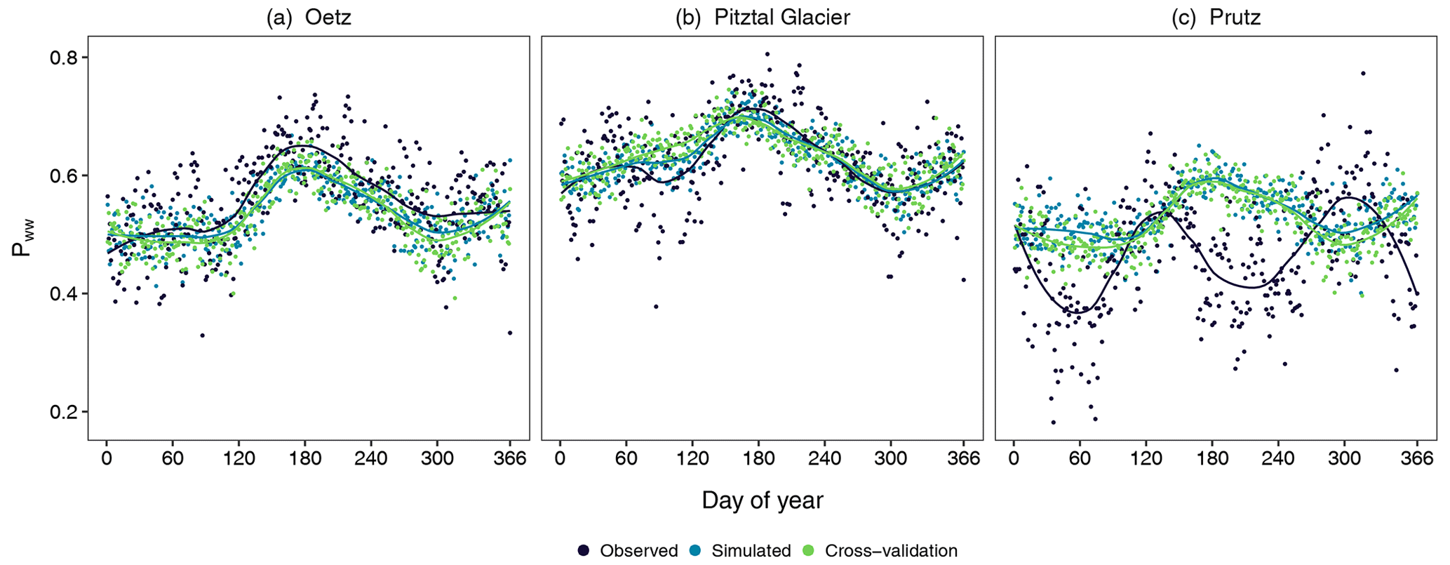
Figure 3 The same as Fig. 2 but for the daily conditional probability of a wet day following a wet day (P_ww).

4.1 Evaluation at individual stations

4.1.1 Daily occurrence probabilities at individual stations

First, we assess the performance of the occurrence model with respect to the daily conditional probabilities on which the model was trained. These are important statistics, as they are associated with the ability of the model to reproduce dry and wet spells. Figure 2 illustrates the annual cycle of the empirical and simulated daily conditional probability of a dry day following a dry day (P_dd) at the three selected stations along with the results of cross-validation for the same variable, whereas Fig. 3 illustrates the daily conditional probability of a wet day following a wet day (P_ww). The solid lines are the curves fitted, using the locally weighted scatterplot smoothing (LOESS) method (Cleveland, 1979), to the observed, simulated, and cross-validated probabilities, respectively. The annual cycle of P_dd is accurately simulated at Oetz and Pitztal Glacier, whereas the model largely underestimates it throughout the year at Prutz. However, the seasonality in P_dd is well captured at Prutz. The annual cycle of P_ww is well captured at Oetz and Pitztal Glacier but slightly underestimated at Oetz during the entire year, whereas the model accurately reproduces the probabilities throughout the year at Pitztal Glacier.

Figure 4 The same as Fig. 2 but for the daily occurrence probability of wet days (P_w).

At Prutz, the model performs badly for P_ww (Fig. 3c). The observed seasonality in P_ww at Prutz is completely different compared with the seasonality at other stations, but this is not reproduced by the model at all. Similar to Prutz, the other two stations (St. Leonhard im Pitztal-2 and St. Martin), which have very different climatic characteristics, also exhibit marked differences (not shown) between the simulated and the observed daily values of P_dd and P_ww. What is noteworthy here is that the magnitude and the seasonality of both P_dd and P_ww at Prutz are close to the magnitude and seasonality of P_dd and P_ww at the valley station (Oetz). Similar behavior is observed at the other two stations with poor performance. This is partly due to the fact that the covariates, which were selected as optimal at the majority of stations, did not optimally represent the statistics at Prutz (nor at the other stations with distinct climatologies). This indicates that the selected set of covariates is unable to reproduce seasonality at all of the stations because a small subset of stations has distinctly different seasonality. Furthermore, the performance of the model at Prutz is influenced by the climate characteristics at nearby stations, with respect to magnitude and seasonality, and not the other way around. At all other stations, P_dd and P_ww are well simulated. This suggests that the selected harmonics are capable of capturing the seasonality in daily occurrence probabilities. Moreover, the temporal dependency in the occurrence is well reproduced by the covariate Occ_t−1. In general, we find that the performance of the model at valley stations is similar to that at Oetz, and the performance of the model at high-mountain stations is similar to that at Pitztal Glacier.

Cross-validation produces similar results at all three sites for P_dd. Compared with the results with the simulated probabilities, Prutz and Oetz show slightly more underestimation throughout the year, whereas Piztal Glacier has mostly the same results with only minor deviations. For P_ww, Oetz has similar results throughout the year, whereas Pitztal Glacier has deviations in spring and Prutz has deviations in autumn and winter. The seasonal differences are likely due to very different precipitation characteristics at Prutz, which was removed from the model fitting along with Oetz and Pitztal Glacier in cross-validation.

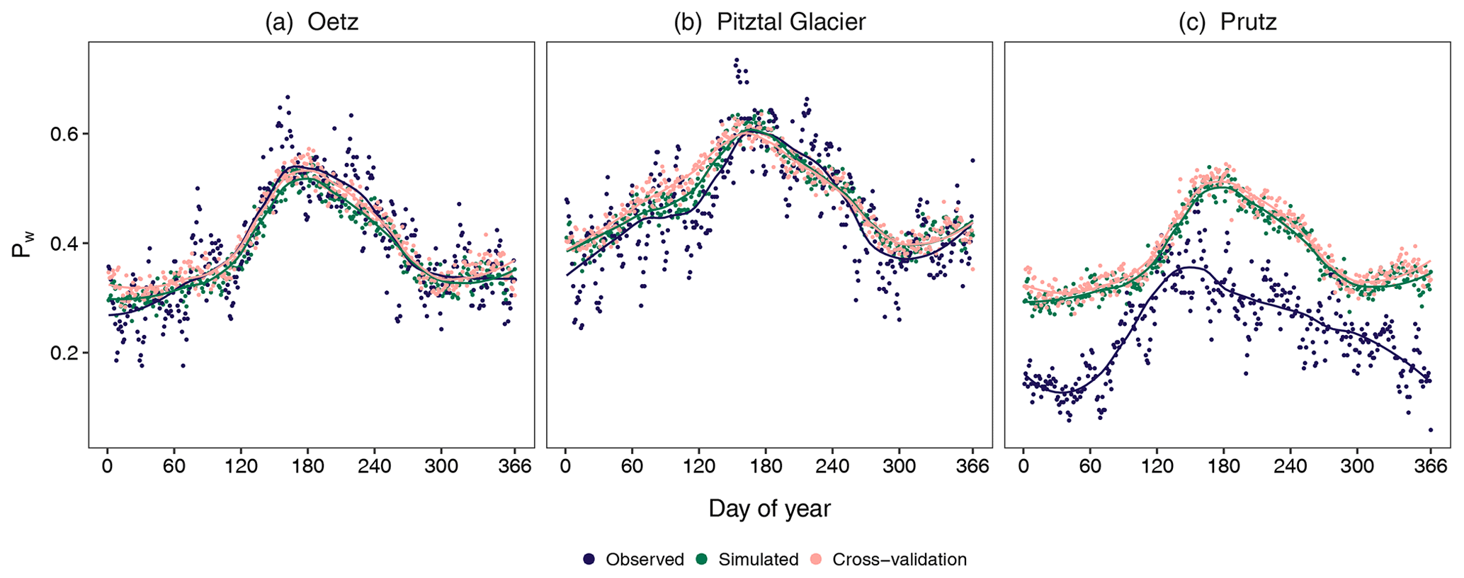
To further examine the ability of the model to reproduce the observed climatology of wet days, we next consider the unconditional daily occurrence probability of wet days (P_w) (Fig. 4). Again, P_w is very well simulated at both Oetz and Pitztal Glacier, and the annual cycle of P_w is well captured by the model. At Prutz, the generator not only largely overestimates the probabilities but is also unable to accurately capture the seasonality. Again, both the seasonality and magnitude in simulated probabilities at Prutz are closer to those of valley stations (such as Oetz). Cross-validation produces similar results at all three sites for P_w with small deviations compared with the simulated results.

The performance metrics for daily occurrence probabilities are shown in Fig. 8a. (Note that the performance metrics are presented for the simulated data and not for the cross-validation.) The metrics are computed for each of the 29 stations and are plotted as a box plot. All of the error metrics as well as the CC and R² suggest that the best performance is seen for P_dd, followed by P_w and then P_ww. The high CC and R² values for P_dd and P_w demonstrate the overall very good performance for these two statistics. Conversely, the small CC and R² values for P_ww indicate relatively poor model performance. This is – at least partly – due to the fact that the model performs very poorly with respect to generating precipitation series at the stations with distinct climatologies (see Fig. 3c).

4.1.2 Frequency of spells of different lengths at individual stations

Another important feature of the model is its ability to simulate long sequences of wet and dry days. Here, we examine the ability of the model to simulate wet and dry spells of different lengths at individual stations. Figure 5 displays the frequency of wet spells at the selected stations with a length of 2 to 15 d. The precipitation generator is able to reproduce wet spells of different lengths at the valley and high-mountain stations accurately. The shaded region is the tolerance interval ${\mathrm{TI}}_{\mathrm{99}}^{\mathrm{95}}$ of the 30 realizations. The observed values of the spells of different lengths are within the TI, showing that the model does an excellent job of reproducing even the longer spells. It is noteworthy that the model captures the spells very accurately, even if it is not trained on these statistics. There are very few occurrences of wet spells longer than 10 d at the majority of stations in the observed data, albeit they are also well reproduced. At Prutz, the model overestimates wet spells of all lengths. The observed values of the spells are not within the ${\mathrm{TI}}_{\mathrm{99}}^{\mathrm{95}}$, indicating a consistent overestimation in all 30 realizations. This overestimation occurs because the model is unable to reasonably reproduce the conditional probabilities of P_ww at Prutz. In fact, the large overestimation of P_w at Prutz (Fig. 4) ultimately contributes to the overestimation of wet spells. Again, cross-validation produces similar results.

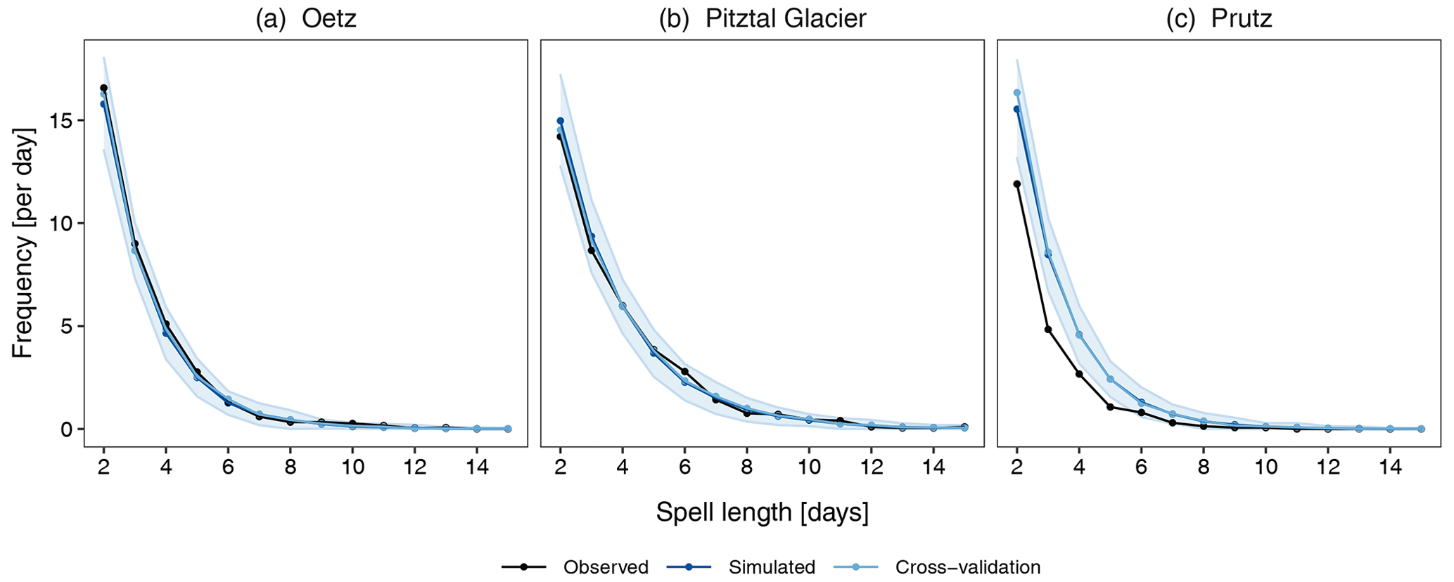
Figure 5 The frequency of wet spells of different lengths at three selected stations: (a) Oetz, (b) Pitztal Glacier, and (c) Prutz. The frequency of the observed spells is obtained from the observed 30 years (1981–2010) of data. The frequency of the simulated spells is determined for each of the 30-year simulations separately and averaged over the 30 realizations. The shaded region is the selected tolerance interval ${\mathrm{TI}}_{\mathrm{99}}^{\mathrm{95}}$ for the simulated values of the 30 realizations. The two-sided TI is specified for 99 % of the population and with a 95 % confidence level. Note that the TIs are not presented for cross-validation.

Figure 6 The same as Fig. 5 but for the frequency of dry spells of different lengths.

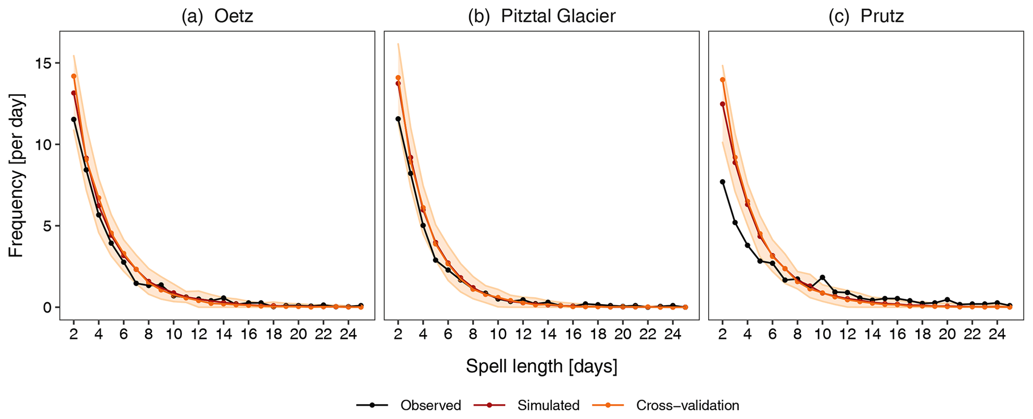
Figure 6 demonstrates the frequency of dry spells with lengths from 2 to 25 d at the three selected stations. The model is able to simulate dry spells of all different lengths at the valley and high-mountain stations with great accuracy. There are very few occurrences of extreme spells longer than 15 d in the observed data, although these are also reproduced well by the model. At Prutz, the model overestimates spells shorter than 4 d but does a very good job for the longer spells. Again, the shaded regions are the statistical tolerance level ${\mathrm{TI}}_{\mathrm{99}}^{\mathrm{95}}$ of the 30 ensembles. The observed values of the spells are within the tolerance region except for the shorter spells (even at Prutz). The worst performance for both wet and dry spells is observed at Prutz. In general, the model does a better job for valley stations than for high-mountain stations (not shown). The previous day's occurrence as a covariate (Occ_t−1) is able to simulate long sequences of both wet and dry days very well at the majority of stations with great accuracy. The occurrence model satisfactorily reproduces the occurrence pattern at the majority of the stations, except at the few distinct stations with peculiar climatologies. Again, the results of the cross-validation are similar.

With respect to wet and dry spells, the model performance is mostly similar for both events (Fig. 8b) except that the RMSE is generally larger for the former, suggesting slightly worse overall performance for wet spells. The CC and R² values are nearly 1, indicating excellent model agreement with the observations for both dry and wet spells.

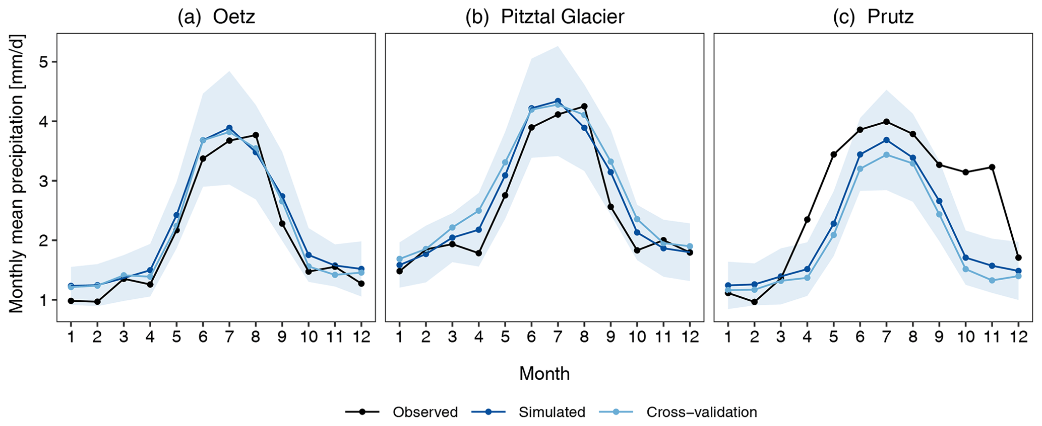
Figure 7 Monthly mean precipitation (mm d⁻¹) at the three selected stations: (a) Oetz, (b) Pitztal Glacier, and (c) Prutz. The observed values are obtained from the observed 30 years (1981–2010) of data, and the simulated values are the mean of the 30 realizations. The shaded region is the selected tolerance interval ${\mathrm{TI}}_{\mathrm{99}}^{\mathrm{95}}$ for the simulated 30 realizations.

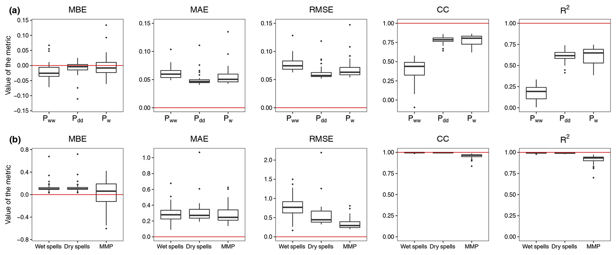
Figure 8 Performance metrics for the model at individual stations for the (a) daily occurrence probabilities (P_dd, P_ww, and P_w) and the (b) frequency of dry spells and wet spells of different lengths and monthly mean precipitation (MMP). The unit for the MBE, MAE, and RMSE for wet and dry spells is per year (yr⁻¹), and the unit for MMP is millimeters per day (mm d⁻¹). The red horizontal line in each panel corresponds to the optimal performance for the corresponding metric.

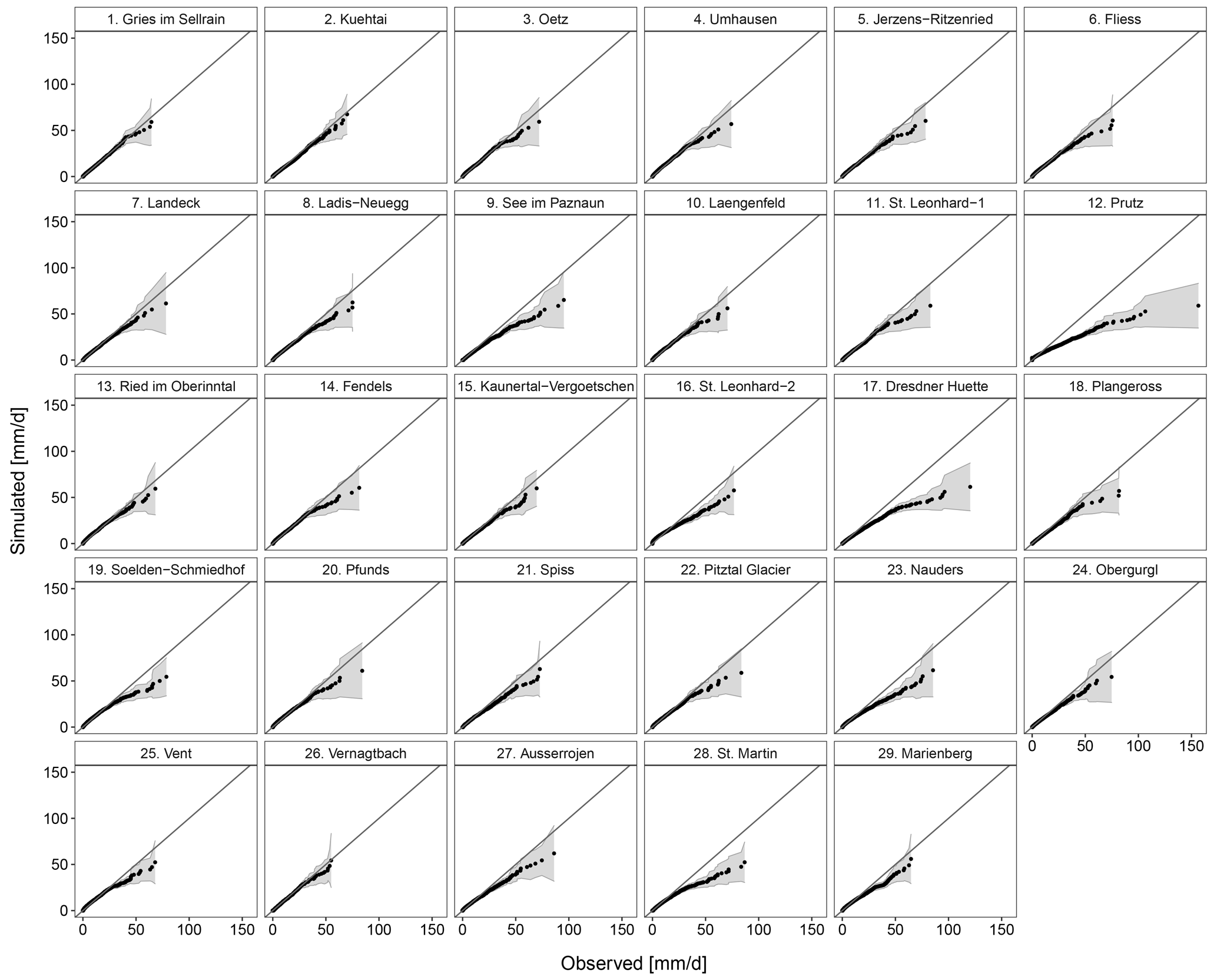
Figure 9 Quantile–quantile (Q–Q) plot showing the percentiles of daily precipitation at each of the 29 individual stations (Table 1). The shaded region is the selected two-sided tolerance interval ${\mathrm{TI}}_{\mathrm{99}}^{\mathrm{95}}$ for the simulated 30 realizations. The black solid line in each panel plot corresponds to the 1:1 line.

4.1.3 Monthly mean precipitation at individual stations

An important aspect of the precipitation generator is its ability to reproduce the amount of precipitation observed at the stations. As the model for amount is the gamma distribution at the observed locations, the mean, which is the product of the shape and scale parameters of the gamma distribution, should be well reproduced. Figure 7 displays the monthly mean precipitation for the observed and simulated data at the selected stations along with the results of the cross-validation. At both Oetz and Pitztal Glacier, the model is able to reproduce the mean very well, as the observed values are within the ${\mathrm{TI}}_{\mathrm{99}}^{\mathrm{95}}$ (the shaded region). At Prutz, the model underestimates the mean in April, May, October, and November, whereas it is able to reproduce the mean reasonably well in other months, as the observed values are within the ${\mathrm{TI}}_{\mathrm{99}}^{\mathrm{95}}$. The results for cross-validation are similar at all three stations; however, compared with simulated data, Pitztal Glacier and Prutz show slight deviations. The performance metrics are displayed in Fig. 8b. For the monthly mean precipitation, the model performs very well, as can be seen by the small magnitudes of the errors (typically less than 0.5 mm d⁻¹) and the strong CC and R² values.

4.1.4 Quantile–quantile (Q–Q) plots at individual stations

Here, we examine the Q–Q plots at each individual station for which observed data are available (Fig. 9). It can be seen that the distribution of precipitation is accurately simulated at the majority of stations. The largest discrepancy between the observed and simulated distributions is found at Prutz; this station has the largest spread in the observed data, and this is not reproduced well by the model. Apart from that, there are some stations, including Dresdner Huette, where the higher quantiles are not well reproduced. These are stations that have longer tails in the precipitation distribution in the observed data. This is a commonly reported problem in the literature: the gamma distribution is not adequate to simulate extremes.

We further examine the distributions of the generated data for each month at each of the 29 stations using a Kolmogorov–Smirnov test and a Wilcoxon–Mann–Whitney test. The results are shown in the Supplement (Figs. S1, S2). As revealed by the Q–Q plots, the worst performance is observed at Prutz, St. Martin, and St. Leonhard im Pitztal-2, which have distinct climatologies.

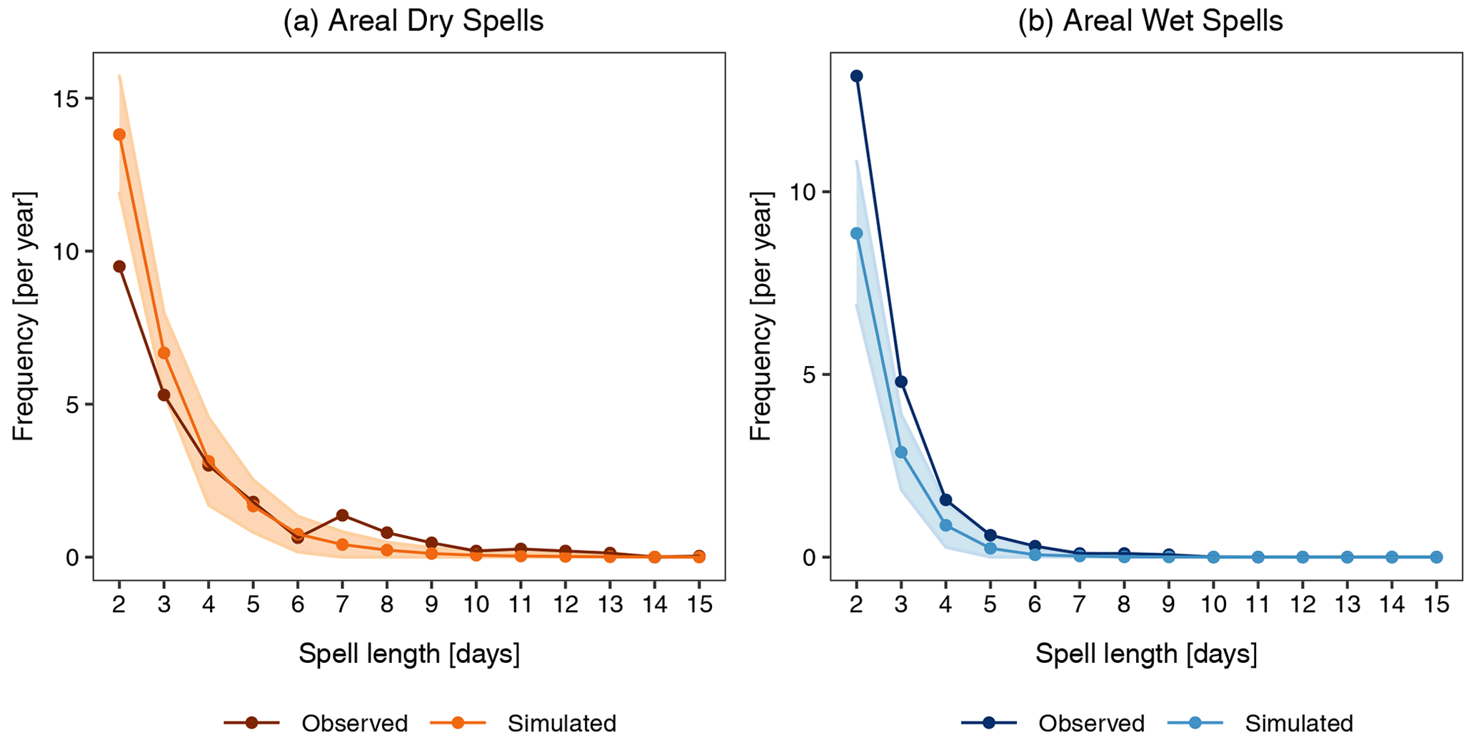
Figure 10 The frequency of the areal spells of different lengths (see Sect. 4.2.1) for (a) dry spells and (b) wet spells. The observed spells are obtained from the 30 years (1979–2008) of APGD gridded data. The simulated spells are the mean of the 30 realizations. The shaded region is the selected tolerance interval ${\mathrm{TI}}_{\mathrm{99}}^{\mathrm{95}}$ for the simulated data. The two-sided tolerance interval is specified for 99 % of the population and with a 95 % confidence level.

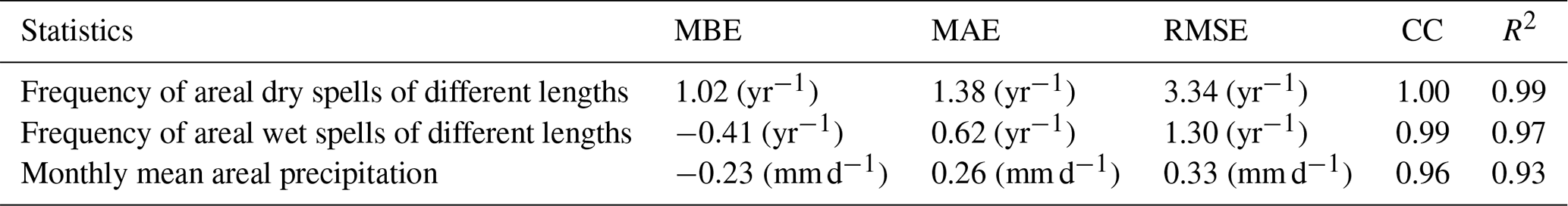
Table 3 Performance metrics of the gridded model for reproducing areal statistics.

4.2 Evaluation of simulated gridded data

In this section, we focus on evaluating the spatial dependence structure in the simulated data, which is an important aspect for many hydrological applications. Here, we present the results of the validation – first for the spatial statistics related to the occurrence and then for the occurrence and amount combined. More details on this aspect of validation are given in Sect. 5.

4.2.1 The frequency of areal spells of different lengths

One of the most challenging features of the gridded precipitation generator is its ability to reproduce the areal spells of wet and dry days of different lengths. This is one of the sought-after features in agricultural and hydrological applications. We define an areal wet (dry) spell as the number of consecutive days on which 95 % of the study area is wet (dry). Figure 10 illustrates the areal spells of dry and wet days of different lengths in the observed and simulated data. It can be seen that the areal dry spells are better simulated than the areal wet spells. The areal dry spells longer than 2 d are accurately simulated, whereas the areal dry spells of 2 d are overestimated. For areal wet spells, the model underestimates spells of all lengths. Larger discrepancies are found for shorter spells.

For the areal spells, the performance metrics are shown in Table 3. For areal dry spells, the error statistics suggest that the model has a tendency to overestimate the spells. This is because the model largely overestimates shorter areal dry spells. The CC is perfect and the R² is also nearly 1, suggesting excellent model performance. For areal wet spells, the error metrics (the MBE, MAE, and RMSE) are small; here, a negative MBE value indicates overall underestimation of wet spells, and strong CC and R² values suggest very good agreement with the observed values.

4.2.2 Spatial distribution of occurrence probabilities

The spatial distribution of the simulated probabilities of wet days (P_w) for each season (Fig. 11a, d, g, j) is compared to that of the (gridded) observations (Fig. 11b, e, h, k). It is noteworthy that the model-generated data have a 1 km spatial resolution, whereas the observed gridded data have a 5 km resolution. The model is able to generate the seasonality in the spatial distribution of P_w very well. In particular, the higher probabilities in spring and summer are well reproduced. Moreover, at a 1 km resolution, the influence of topography on the spatial distribution of P_w is clearly visible. This is due to the inclusion of elevation in the kriging interpolation.

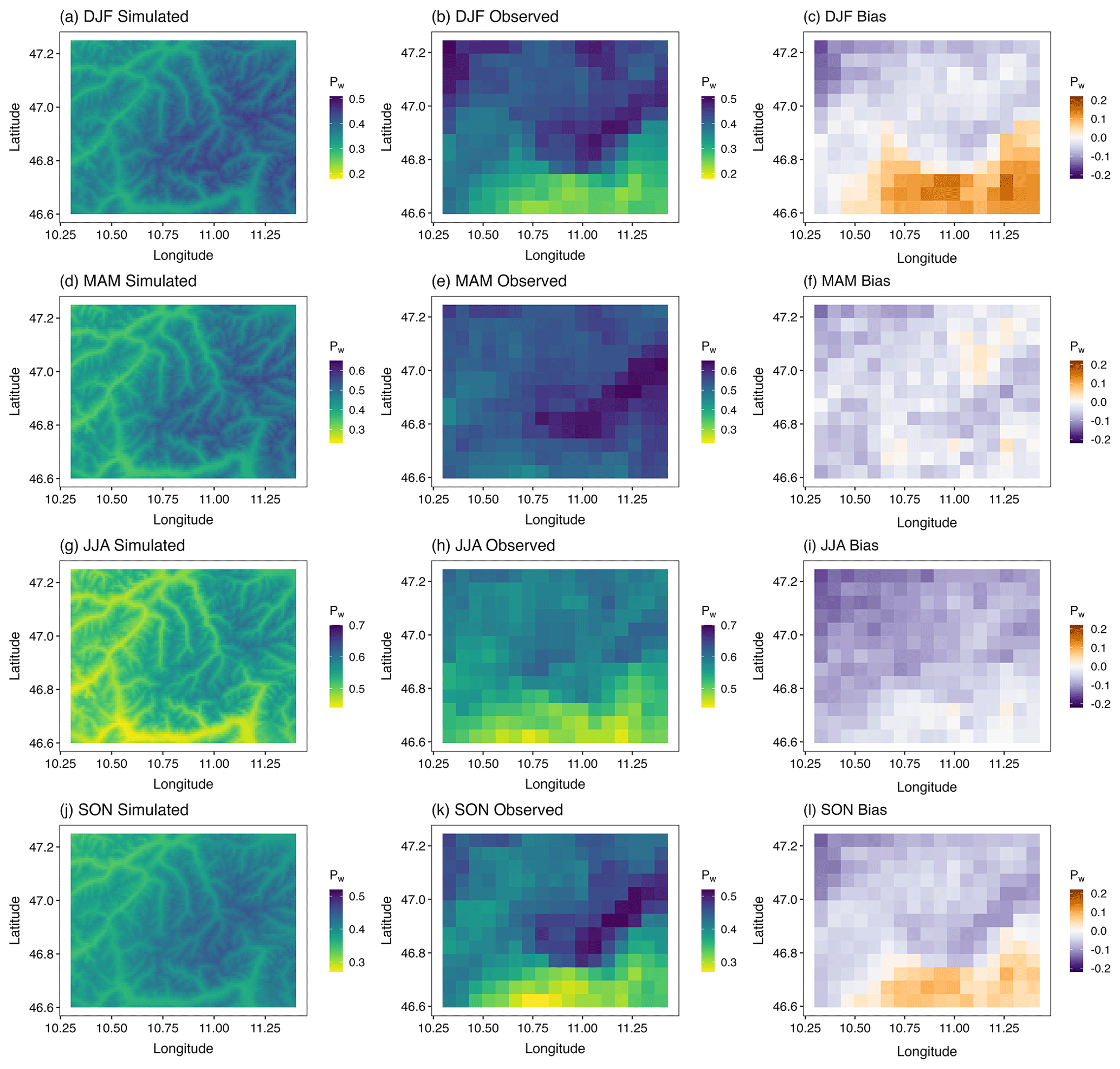
Figure 11 Spatial distribution of the occurrence probability (P_w) in four seasons in the simulated 30 realizations (a, d, g, j) and the 30 years (1979–2008) of observed APGD gridded data (b, e, h, k) as well as the bias (simulated − observed) in the simulated data (c, f, i, l). The spatial resolution of the APGD data is 5×5 km. Note the different scales in the color coding for the different seasons.

To test the model performance at each grid point, we upscale the simulated data from 1 to 5 km, and the difference between the observed and the simulated data is shown in Fig. 11c, f, i, and l. It can be seen that the biases are small in spring and summer and are mostly similar throughout the domain. However, there is an overestimation in the southeastern part of the region and a slight underestimation in the northwestern part in winter. The overestimation in the southeastern part of the study area is because the station density is low in that part of the area. There is one station (St. Martin) which is heavily influencing the aforementioned area, and it has the highest probability of precipitation occurrence, which is manifested through the spatial interpolation of the model parameters via kriging (Sect. 2). Except for summer, this station has a much higher probability of precipitation occurrence relative to the other stations. This is also reflected by the fact that, in the simulation, the bias is mostly zero in the southeastern part of the region in summer.

Figure 13a illustrates the performance metrics for the spatial distribution of P_w for each month. All three error statistics are within 0.1, suggesting very good model performance. The largest errors are for August, during which time a negative MBE indicates an overall underestimation of P_w, whereas the largest overestimation is found in February. The lowest overall bias is found in September. The highest CC and R² values are observed in May. In colder months, i.e., in winter and autumn, the correlations between the observed and simulated probabilities are weak and the R² is also small, suggesting poor performance for these months. The worst performance is observed in January, during which time the CC and R² values are almost 0, whereas the best performance is found in May.

4.2.3 Spatial distribution of mean wet-day daily precipitation

Next, we consider the mean wet-day daily precipitation in order to assess the ability of the model to reproduce the observed climatology of the precipitation amount over the region. We consider the mean daily precipitation on wet days in each season over the 30 years of the simulated 30 ensembles, i.e., 900 years of data at each grid point (Fig. 12a, d, g, j), and compare it to the observations (Fig. 12b, e, h, k). Figure 12c, f, i, and l depict the bias in the simulated and observed values at each grid point. The model is able to simulate the spatial seasonal variability in precipitation very well. In particular, the summer precipitation due to the convective processes and thunderstorms, which account for high amounts of precipitation, is well reproduced. In the colder seasons (December–January–February, DJF, and September–October–November, SON), the precipitation amount in the simulated data has visibly less dependence on elevation; hence, the generator has a tendency to generate less spatial variability in the daily precipitation amount across the region. In contrast with the largely overestimated spatial probability of occurrence in the southeastern part of the study area (Fig. 11), the model underestimates the precipitation amount. St. Martin not only has a high frequency of wet days but also the highest precipitation amount in all seasons among the 29 stations. The gamma distribution is unable to reproduce the large precipitation amount at this station, resulting in an underestimation of the precipitation amount in the surrounding area as well.

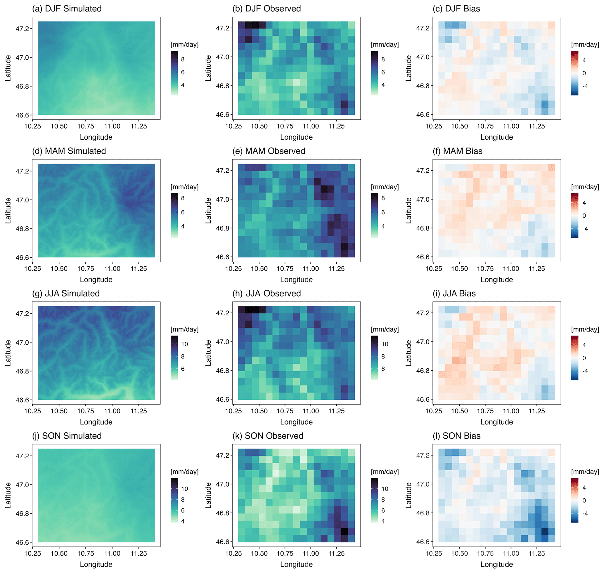
Figure 12 Spatial distribution of the mean wet-day daily precipitation amount for four seasons (mm d⁻¹) for the simulated (a, d, g, j) and observed (b, e, h, k) data as well as the bias (simulated − observed) in the simulated data (c, f, i, l). The mean wet-day daily precipitation is obtained at each grid point for each season in each of the 30 realizations, and the average of the 30 realizations is shown. The spatial resolution of the simulated data is 1×1 km, whereas the spatial resolution of the observed data is 5×5 km. Note the different scales in the color coding for the different seasons.

Another important aspect to note with respect to the observed APGD data is that the probabilities of wet days in the southeastern part of the region in the colder seasons are low (Fig. 11), whereas the precipitation amount is high in the same part of the region – particularly in SON (Fig. 12). The model fails to capture this behavior. This is also because the model has to extrapolate the parameters in this part of the study area, as there is no observed station present beyond St. Martin. Hofstra et al. (2010) found that the density of the station network used for interpolation influences the distribution of precipitation and the areal mean amount of precipitation. They reported that when fewer stations are used, precipitation is oversmoothed, leading to a strong tendency for interpolated values to be less than the “true” value, and that the effect was largest for higher percentiles. Dresdner Huette also has a larger precipitation amount in the observed data in autumn (and also in winter) compared with other stations. Moreover, the model underestimates the precipitation amount in the region surrounding this station, mainly in SON (see the northeastern part in SON in Fig. 12). Another reason for the underestimation in autumn could be the inability of the model to simulate orographic precipitation particularly related to föhn events. These factors combined lead to a large underestimation in this region in autumn.

Figure 13b depicts the performance metrics for the spatial distribution of mean wet-day daily precipitation for each month. The MBE, MAE, and RMSE are the largest in November, and the negative MBE value of approximately −2 mm d⁻¹ suggests a large underestimation in that month. For October, a large underestimation is also found, whereas the smallest error metrics are found in March, followed by February. High CC and R² values are observed in February and March, suggesting the best performance in these months, whereas the worst performance is found in September. Contrary to the bad performance for the spatial distribution of P_w, the spatial distribution of mean precipitation is better reproduced in winter (compare panels c, f, i, and l of Figs. 11 and 12).

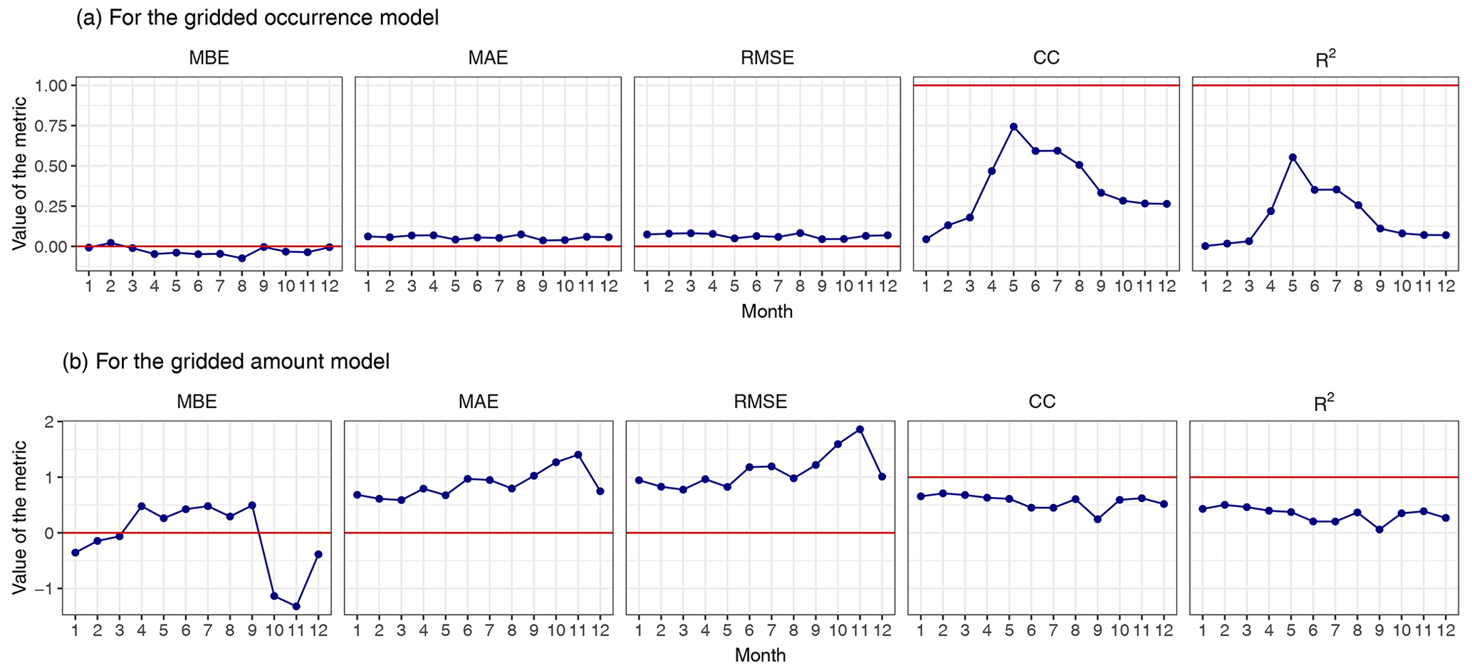
Figure 13 Performance metrics for the gridded model for the (a) spatial distribution of probabilities of wet days (P_w) in each month and the (b) spatial distribution of mean wet-day daily precipitation. The unit for the MBE, MAE, and RMSE is millimeters per day (mm d⁻¹). The red horizontal line in each panel corresponds to the optimal performance for the corresponding metric.

4.2.4 Monthly mean areal precipitation

Next, we assess the ability of the precipitation generator to provide an areal climatology of the precipitation amount. This is also one of the desired characteristics for impact modeling. Figure 14 displays the areal precipitation mean for each month in both the observed and simulated gridded data. The precipitation generator simulates the mean areal precipitation in all seasons with good accuracy (except in autumn), with observed values within the ${\mathrm{TI}}_{\mathrm{99}}^{\mathrm{95}}$. As seen in the spatial distribution of the amount of precipitation (Fig. 12), the model underestimates the areal precipitation in autumn, mainly in October and November. The statistics are shown in Table 3. The small negative MBE value indicates an overall slight underestimation, and the MAE and RMSE are also small (approximately less than 0.4 mm d⁻¹). The high CC and R² values show that the model-estimated means are in very good agreement with the observed values.

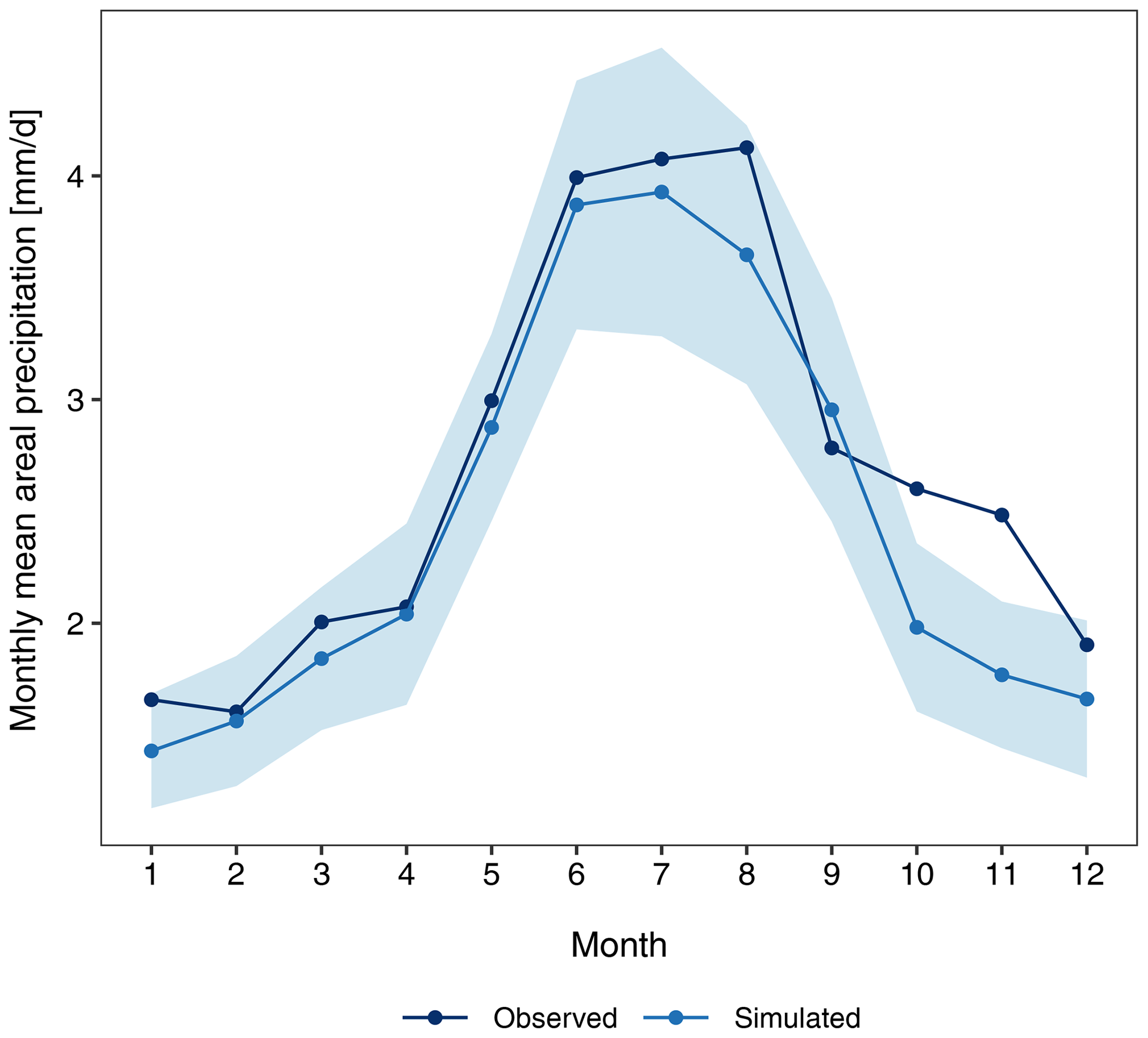
Figure 14 Monthly mean areal precipitation (mm d⁻¹). The observed values are obtained from the 30 years (1979–2008) of observed APGD data, and the simulated values are the mean of the 30 realizations. The shaded region is the selected two-sided tolerance interval ${\mathrm{TI}}_{\mathrm{99}}^{\mathrm{95}}$ for the simulated data.

4.2.5 Annual maximum precipitation sums

Here, we assess the ability of the model to reproduce extreme precipitation amounts. We consider the annual maximum daily precipitation at 29 sites. The daily sum of the observed daily precipitation at 29 sites is obtained, and the maximum of the daily sum in every year is shown as a box plot in Fig. 15. For the simulated data, the time series of daily precipitation for 30 years at the nearest grid point to the 29 observation stations is extracted from the gridded data for each of the 30 realizations. The sum of the daily precipitation at the 29 sites in the simulated data is obtained, and the maximum in each year is presented as a box plot in Fig. 15. There is an underestimation in the simulated maximum precipitation sums. The median is underestimated by approximately 20 %. The inter-annual variability in the maximum precipitation sums is also underestimated, as can be seen from the interquartile range (IQR). However, the range of the box plot of the model-simulated values is larger than that of the observed values, with extreme outliers suggesting that the model generates higher extreme precipitation sums than those in the observed dataset. In general, the model is able to generate extreme precipitation reasonably well.

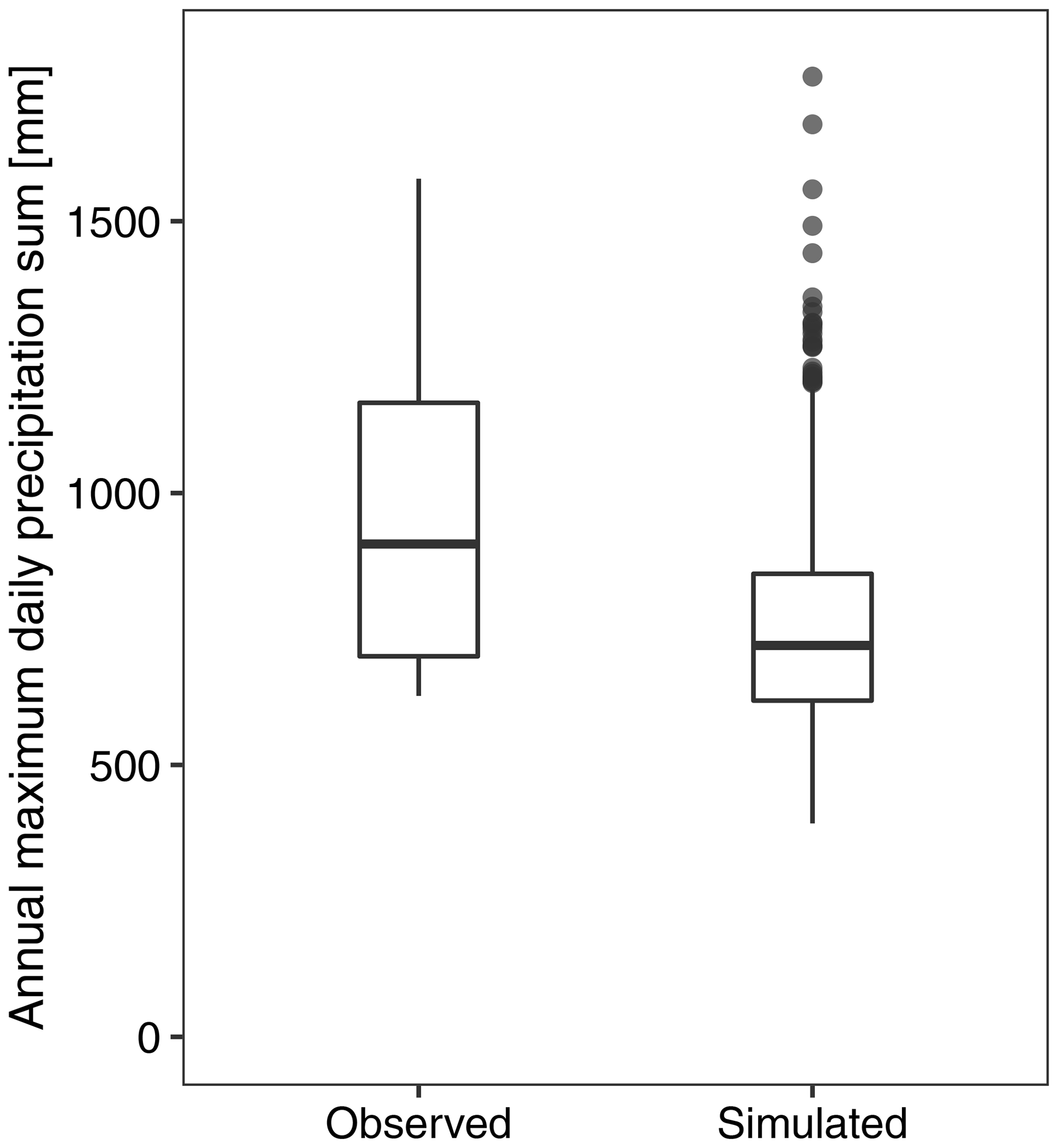
Figure 15 The annual maximum daily precipitation sum at the 29 sites for the observed and simulated data. The sum of daily precipitation at the 29 sites is obtained, and the maximum in each year is presented as a box plot. Thus, the box plot for the observed data is based on 30 values, whereas is based on 900 values (30 realizations of 30 years) for the simulated data.

4.3 Comparison between the anisotropic and isotropic models using KED and OK

Here, we compare the results of our simulations, i.e., using KED in the anisotropic model (Aniso–KED) with three different model setups: (i) considering OK in the interpolation of the parameters of the anisotropic model (Aniso–OK), (ii) using the original isotropic model that utilizes OK for the interpolation of the parameters (Iso–OK), and (iii) using the isotropic model with KED (Iso–KED). We examine the results for the monthly sum of the areal mean daily precipitation in these four simulation cases (experiments) with the observed APGD gridded data. Figure 16 displays the distributions of the monthly sum of the areal mean daily precipitation for the simulated 900 years for each of the four experiments and the observed 30 years of gridded data.

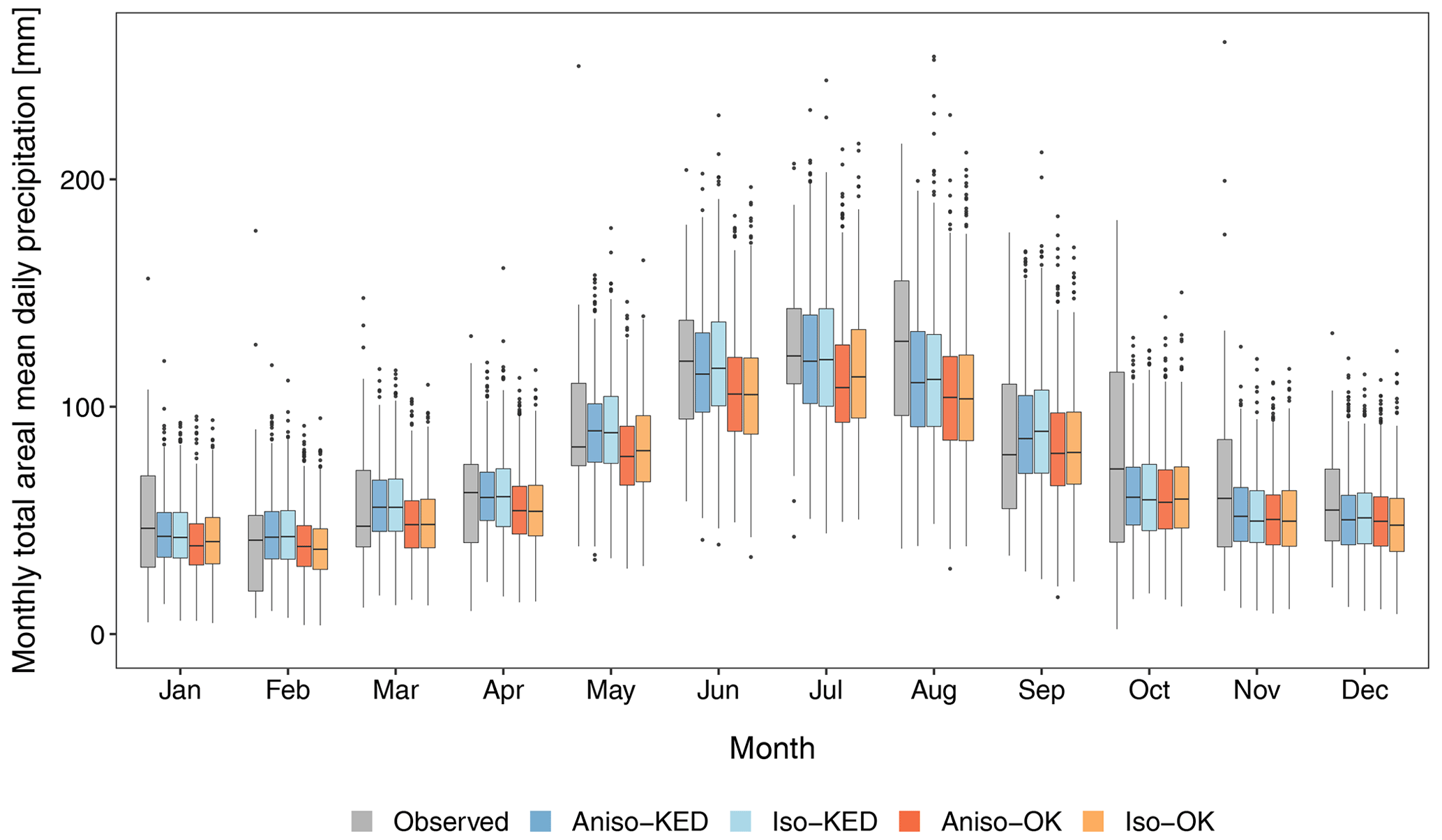
Figure 16 Monthly sum of the areal mean daily precipitation (mm) for each month in the 30 years (1979–2008) of observed APGD data and the simulated 900 years (30 realizations of 30 years) of data for the four experiments: Aniso–KED, Iso–KED, Aniso–OK, and Iso–OK (see the text for specifications).

The model performance of Aniso–KED and Iso–KED is mostly similar in all months, whereas the model performance of Iso–OK and Aniso–OK is similar in all months. The model performance varies greatly from month to month for all four experiments, but both experiments involving KED (Aniso–KED and Iso–KED) outperform those using OK in the vast majority of months. It is evident that allowing elevation as a covariate in the kriging interpolation for prediction at each grid point appreciably improved the amount of precipitation in most months.

The median for both of the KED experiments is overestimated in February, March, May, and September, whereas the median is underestimated in the rest of the months. The IQR in Fig. 16 shows the inter-annual variability (IAV), but the figure also shows the intra-seasonal and inter-seasonal variability. The model reproduces the intra-seasonal and inter-seasonal variability very well in all four experiments, but it generally performs better for the experiments in which KED is employed. The IAV is better simulated in summer than in colder months. The best performance is found in July, when the variability is larger in the simulated data for all four experimental setups compared with the observed data. Furthermore, the median in July is very close to the observed value for both of the simulations using KED. This is remarkably good performance, as WGs are typically criticized as having the tendency to underestimate the low-frequency variability, as is the case for most of the months in our precipitation generator. Conversely, for all four experiments, our model is unable to reproduce the larger IAVs in other months (particularly October). This could also be one of the reasons for the large underestimation of the precipitation amount over the study area in autumn, as discussed in the previous sections. It is noteworthy that the model performance is essentially similar from October to December in all four experiments. This shows that, regardless of the type of correlation structure and the interpolation method, the model is unable to capture the spatial distribution of precipitation in those months. In general, the model performance is better in warmer months than in colder months.

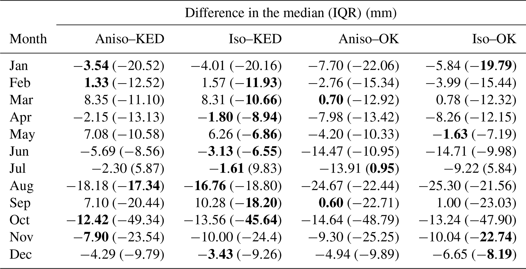
The differences in the observed and simulated median and IQR in each month for each of the four experiments are listed in Table 4. Overall, the experiments with KED outperform those using ordinary kriging, and the Iso–KED combination is slightly superior to the fully anisotropic combination. Apparently, even for a small region in complex terrain, such as the present study area, isotropic covariance is adequate to reproduce the precipitation fields. In the observed data, anisotropy is indeed present, but the difference between the variation in the correlations with horizontal distance and the variation in the correlations with vertical distance is very small. Hence, there is almost no difference in the performance of the model in the isotropic and anisotropic formulations. The two experiments with OK not only underestimate the amount of precipitation but also lack the topographical influence on the simulated precipitation amount and rather produce smooth precipitation fields over the region (see Fig. S3). However, the influence of topography must be included in the model in order to realistically simulate the precipitation fields, as we have shown here by considering KED interpolation.

Table 4 Difference (simulated − observed) in the median and interquartile range (IQR) of the observed and simulated monthly sum of the areal mean daily precipitation (mm) in each month and each of the four experiments. The bold values indicate the best model performance in each month.

As for the occurrence model, the covariance structure has a slight influence on the model performance. Figure 17 compares the areal dry and wet spells for all four experiments with those observed. The performance of the anisotropic model is better for dry spells: Aniso–KED performs sightly better than Aniso–OK. In contrast, the performance of the isotropic model is better for wet spells: Iso–KED performs slightly better than Iso–OK. For both areal dry and wet spells, KED interpolation adds little value to the simulation over using OK.

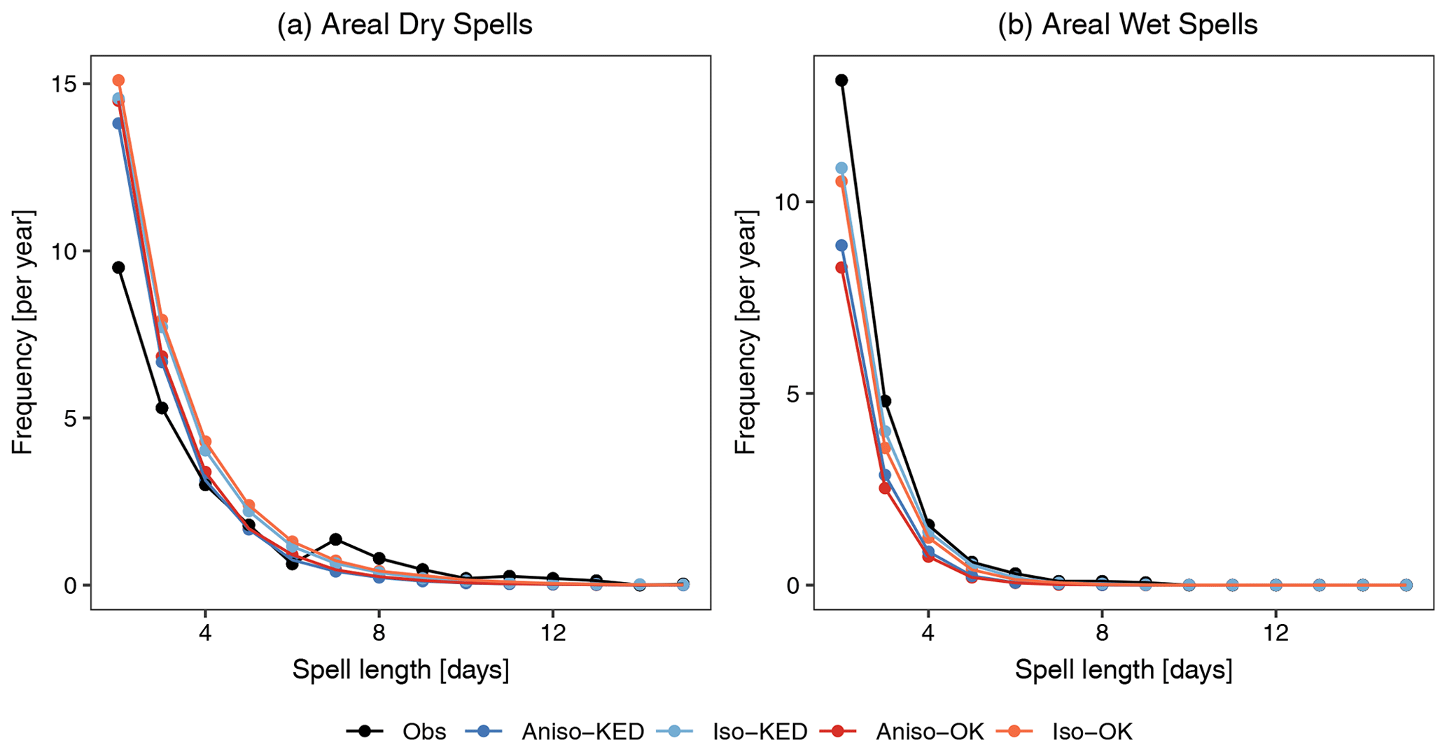
Figure 17 The frequency of areal spells (yr⁻¹) of different lengths in each of the four experiments with 900 years of simulated data and with 30 years (1979–2008) of observed APGD data for (a) areal dry spells and (b) areal wet spells. For the simulated dry and wet spells, their frequency is determined for each of the 30-year simulations separately and averaged over the 30 realizations.

5 Discussion

In this study, we have tested two extensions of the original isotropic framework of Kleiber et al. (2012) for the simulation of precipitation fields: (i) the inclusion of anisotropy in the covariance function and (ii) the application of KED in the interpolation of the parameters (instead of OK). Our model adds substantial value over the original model in a highly complex mountainous region in the Austrian Alps. As a statistical downscaling tool, this model does not require any large computational resources. Obviously, compared with a single-site WG, it requires additional computing resources, but it is still very parsimonious and fast compared with dynamical downscaling models. It can be easily run on any high-end personal computer. In terms of model complexity, our model only has two parameters more than the original model: the two range parameters in the vertical direction due to the inclusion of elevation in the covariance functions of the occurrence and amount models, respectively. Hence, in terms of computational time, the proposed model takes approximately 8 % longer than the original model to complete a run, which includes model fitting and simulation.

The major improvement in the results from our model comes from the KED interpolation, rather than the included anisotropy in the covariance structure. This suggests that there is no strong directional dependency in the precipitation simulation. Although there are minor differences in model performance using the isotropic and anisotropic covariance functions, it can be concluded that an isotropic covariance function is sufficient, even for small-scale topographic variability such as that in the present study in the European Alps. However, the topographical details must be included in the interpolation of the parameters of the model. Similar results can be expected for complex terrain in other mountainous regions.

At individual locations with observations, the model satisfactorily reproduces various observed statistics and the overall distribution of precipitation. The model is also able to capture spatial and temporal variability over the entire region reasonably well. It is capable of simulating the dry-day statistics over the whole region very well; however, an underestimation is observed for the wet-day statistics. The frequency of the areal dry spells of 1 or 2 days is strongly overestimated. The model uses the previous day's occurrence as a covariate, which creates a first-order two-state Markov chain at an individual location. Dabhi et al. (2021) applied a first-order two-state Markov chain model at stations covering different climate zones in Europe and found that it had a tendency to overestimate dry spells. The first-order Markov chain uses the occurrence from only 1 day in the past; however, there may be longer-lasting correlations present in the data. Considering the occurrence from 2 or more days in the past, i.e., forming a second-order or higher-order Markov chain, at individual locations may potentially improve the results for both dry and wet spells. For example, Wilson Kemsley et al. (2021) studied the order of Markov chains in different climate regimes across the world and showed that a third-order model reproduces observed dry-spell distributions the best. Alternatively, allowing other meteorological variables, such as wind speed and humidity, as covariates in the GLM can also improve the results (Ataharul Islam and Chowdhury, 2006).

The model captures the month-to-month variability in the monthly sum of precipitation very well due to the use of the time-dependent harmonics of sine and cosine as covariates in the modeled spatial covariance structure. However, the inter-annual variability is largely underestimated, mainly for the colder months. Even if we adopt the NAOI as a covariate to alleviate the well-known problem of overdispersion in this type of model, overdispersion remains an issue. One reason for this is the tendency of the model to underestimate large daily precipitation amounts. This is because the model generates the precipitation amount using a transformed Gaussian process that reduces to a gamma distribution at individual locations. The gamma distribution is not a heavy-tailed distribution and is, therefore, not well suited to reproducing heavy precipitation. However, Wilks (2009) also reported the underestimation of heavy precipitation using a mixture of two exponential distributions to account for both smaller and larger precipitation amounts. This is another commonly reported problem for precipitation generators (e.g., Wilks, 1999; Furrer and Katz, 2008). Allowing heavy-tailed distributions alleviates overdispersion (Serinaldi and Kilsby, 2014), but simulating spatial extremes and successfully capturing smaller precipitation amounts with such a simple model is even more challenging. Another way to reduce overdispersion is by allowing a suitable covariate, such as seasonal total precipitation, in the GLM, as shown by Kim et al. (2012), or by including seasonal dry/wet indicators, as in Kim and Lee (2017). Verdin et al. (2018) modified the model of Kleiber et al. (2012) by allowing the domain-averaged seasonal total precipitation as a covariate and showed that the inclusion of this covariate improved the simulation. However, their study was focused on flat terrain, where it is promising to take the areal precipitation as a covariate for the whole domain. This may not be suitable for mountainous terrain, and location-specific climate information might, instead, be more promising. In this study, we wanted to evaluate the model with respect to its ability to reproduce the observed statistics at locations where no observations are available; thus, we avoided the inclusion of any location-specific information so that the model was not conditioned upon the availability of information at each grid point. We believe that the model performance could be improved by allowing such gridded information as a covariate.

In complex mountainous terrain, individual stations can exhibit precipitation characteristics quite distinct from those of neighboring (or more distant) stations with more typical characteristics. A station-by-station evaluation (Sect. 4.1) revealed that the model cannot reproduce precipitation at these distinct stations (e.g., Prutz in Figs. 2–7). For the gridded simulations, we would have expected that these distinct stations might negatively influence their neighboring stations. In contrast, however, the nearby stations influenced the distinct stations by generating overly strong correlations. Figure S4 depicts the inter-station correlations in the precipitation occurrence among the 29 stations in the observed data against the simulated data. The cloud of points with weak correlations in the observed data belongs to the distinct stations, but the correlations are very strong in the generated data. The reason for this is the good density of the network of 29 stations in such a small region. This is also the reason that the largest discrepancy in the performance of both the occurrence and amount models amongst the 29 stations is found at those distinct stations: the model generates the statistics of the nearby stations at those distinct stations, rather than reproducing their own observations. Thus, a distinct station in a region with a dense observational network cannot be reproduced but also does not strongly deteriorate the overall performance with respect to the reproduction of the spatial information. This finding is also confirmed by the holdout cross-validation. As discussed in Sect. 3.2, this is due to the choice of the same set of covariates. Using the same set of covariates is, however, a necessary restriction if the model is aimed at gridded output fields. Reproducing the spatial statistics over the whole region, especially in mountainous regions, is indeed a challenging task; moreover, capturing the realistic spatiotemporal fields of precipitation with such a simple model is even more challenging. Despite this, our model successfully captures many difficult statistics useful for climate change impact applications, such as long spells of dry and wet days and the areal monthly mean precipitation.

However, if a distinct station is located in a data-sparse area (such as St. Martin in our study area), it dominates the entire neighboring region and destroys the spatial structure. Thus, for a spatial precipitation generator in complex terrain, the stations should not only be selected according to data availability (and quality) but also based on their precipitation characteristics. If they have distinctly different precipitation characteristics from the majority of the stations in the region, they should not be included in the training dataset, and if one is explicitly interested in such a station, one should use a single-site approach.

Another limitation of this model is its inability to realistically simulate autumn and winter precipitation. This is because there are systematic differences in the characteristics of weather types between various seasons. In autumn and winter, westerly currents are stronger and the associated precipitation patterns are more pronounced than during spring and summer. The precipitation pattern in winter is associated with dynamically active synoptic-scale weather systems (fronts and low-pressure systems specifically from the North Atlantic Ocean and the Adriatic Sea) in combination with orographic enhancement, whereas the pattern in summer is related to convective activity that is either embedded in frontal systems or generated locally. Our model does not account for the influence of wind on precipitation. This could be the reason for the model not being capable of capturing the spatiotemporal patterns in autumn and winter. The convective season in Austria usually starts in May and lasts until September, and the model successfully captures the spatiotemporal patterns during these months.

The covariance function used in the model is assumed to be stationary, which may not be a realistic assumption. Detecting spatial nonstationarity and modeling it is beyond the scope of this article and will be explored in future research. However, it is possible that the model performance may be improved by considering a nonstationary covariance function (e.g., Paciorek, 2003). As the precipitation–topography relationship is dominant in mountainous regions, the results can also be improved by including not just elevation but also other variables, like slope, aspect, and latitude and longitude, in kriging (Wotling et al., 2000). Considering east–west and north–south gradients of the topography along with elevation in the KED also improves the results (Hiebl and Frei, 2017). As the inclusion of elevation at a 1 km resolution improved the results, we believe that considering an even higher spatial resolution would provide even better simulation of precipitation.

6 Conclusion

A multi-site gridded precipitation generator that provides high-resolution two-dimensional fields of precipitation in complex terrain using historical observations from a network of meteorological stations is developed, implemented, and evaluated. The precipitation generator is an extension of the original framework of Kleiber et al. (2012) that uses a stationary isotropic covariance structure. The original framework is based on a latent Gaussian process for the occurrence and on a transformed Gaussian process for the amount of precipitation in which gamma-distributed random numbers are transformed to normally distributed random numbers. This framework considers the parameters of a generalized linear model (GLM) as a realization of a spatial Gaussian process which allows one to spatially interpolate the parameters using kriging. In this article, two extensions to the original framework are proposed: (i) allowing anisotropy in the covariance structure and (ii) allowing elevation as an external drift in kriging. The anisotropy is included in the model by accounting for the elevation difference in the stationary covariance function of both the occurrence and amount models. Furthermore, elevation is allowed as an auxiliary variable in the kriging equations for the interpolation of the parameters of both the occurrence and amount models.

The model is tested in a small region (about 100×100 km²) with highly complex terrain in the European Alps for which 29 observational stations with 30 years (1981–2010) of data are available. The test region comprises stations with elevation differences of about 2300 m. A total of 30 realizations of 30 years of synthetic gridded data at a 1×1 km² resolution are generated to allow for a robust statistical assessment.

The main findings of this study can be summarized as follows:

• At individual stations where observations are available, the model reproduces the observed statistics realistically well, including annual cycles of daily probabilities of precipitation occurrence and monthly means of precipitation, dry and wet spells of different lengths, and the overall distribution of precipitation amount.

• The model has a great capability to capture the spatiotemporal statistics in complex terrain, including the spatial distribution of occurrence probabilities and amount, areal dry and wet spells of different lengths, monthly mean areal precipitation, and monthly sum of areal daily mean precipitation.

• The proposed extensions considerably improve the simulation of the spatiotemporal fields of precipitation – mainly due to the incorporation of elevation in kriging.

• The use of an isotropic or anisotropic covariance function in the mountainous region is equally good, with marginal trade-offs for some of the statistics.

• The performance of the model varies greatly from month to month, being the best in summer and the worst in autumn.

• Intra-seasonal and inter-seasonal variabilities are well reproduced, whereas inter-annual variability is largely underestimated in autumn and winter.

• At a few of the 29 stations, where the observed precipitation statistics and in particular their seasonality were distinctly different from all of the other stations, the model performance is markedly compromised.

• The underestimation of large amounts of precipitation remains a problem.

Reproducing the spatiotemporal fields of precipitation in a region characterized by complex terrain like the Alps is a challenging task, especially at locations where no observations are available. However, this is an essential requirement for hydrological modeling, as hydrological models are driven by spatially and temporally coherent precipitation data. The proposed model can respond to this need to some extent; nevertheless, further improvement is required, as discussed in the article, to employ the model for downscaling purpose.