the Creative Commons Attribution 4.0 License.
the Creative Commons Attribution 4.0 License.
 | 11 Jan 2022
Technical note: High-accuracy weighing micro-lysimeter system for long-term measurements of non-rainfall water inputs to grasslands
Jon Eugster
Nina Buchmann
Werner Eugster
Non-rainfall water (NRW), defined here as dew, hoar frost, fog, rime, and water vapour adsorption, might be a relevant water source for ecosystems, especially during summer drought periods. These water inputs are often not considered in ecohydrological studies, because water amounts of NRW events are rather small and therefore difficult to measure. Here we present a novel micro-lysimeter (ML) system and its application which allows us to quantify very small water inputs from NRW during rain-free periods with an unprecedented high accuracy of ±0.25 g, which corresponds to ±0.005 mm water input. This is possible with an improved ML design paired with individual ML calibrations in combination with high-frequency measurements at 3.3 Hz and an efficient low-pass filtering to reduce noise level. With a set of ancillary sensors, the ML system furthermore allows differentiation between different types of NRW inputs, i.e. dew, hoar frost, fog, rime, and the combinations among these, but also additional events when condensation on leaves is less probable, such as water vapour adsorption events. In addition, our ML system design allows one to minimize deviations from natural conditions in terms of canopy and soil temperatures, plant growth, and soil moisture. This is found to be a crucial aspect for obtaining realistic NRW measurements in short-statured grasslands. Soil temperatures were higher in the ML compared to the control, and thus further studies should focus on improving the thermal soil regime of ML. Our ML system has proven to be useful for high-accuracy, long-term measurements of NRW on short-statured vegetation-like grasslands. Measurements with the ML system at a field site in Switzerland showed that NRW input occurred frequently, with 127 events over 12 months with a total NRW input of 15.9 mm. Drainage-water flow of the ML was not measured, and therefore the NRW inputs might be conservative estimates. High average monthly NRW inputs were measured during summer months, suggesting a high ecohydrological relevance of NRW inputs for temperate grasslands.
- Article
(10316 KB) - Full-text XML
- BibTeX
- EndNote


Non-rainfall water (NRW) inputs, defined here as dew, hoar frost, fog, rime, and water vapour adsorption, provide water to plants. These different inputs form under different environmental conditions: dew forms on plant surfaces when the temperature of the surface drops below the dew-point temperature of the adjacent air (Beysens, 2018; Monteith, 1957), whereas dew forming directly on soil surfaces is rarely observed (Agam and Berliner, 2004; Ninari and Berliner, 2002). In addition, hoar frost is frozen dew, which forms at temperatures below 0 ∘C. Fog droplets form on condensation nuclei (activated aerosol particles) in the atmosphere when water vapour concentration reaches saturation, whereas rime is supercooled fog in contact with a surface (e.g. vegetation) at a temperature below 0 ∘C. Water vapour adsorption occurs on hygroscopic surfaces, which can lower saturation vapour pressure and thus lead to adsorption, despite the fact that temperatures are still above dew-point temperature (Agam and Berliner, 2006; McHugh et al., 2015).
NRW inputs are a water source for plants during dry periods and can thus have a significant influence on plant–water relations by increasing plant–water status (Boucher et al., 1995; Kerr and Beardsell, 1975; Wang et al., 2019; Yates and Hutley, 1995). Plant–water status is a widely used measure in plant physiology for assessing plant–water stress. It incorporates the amount of water in plants and its energy status (Jones, 2006). NRW inputs can increase the amount of water in plants (Limm et al., 2009; Munné-Bosch and Alegre, 1999) and thereby change the plant–water status, which can lower plant–water stress. Plants can take up NRW via the leaves, termed foliar water uptake (Berry et al., 2014; Eller et al., 2013; Slatyer, 1960), or via the roots (Wang et al., 2019). NRW is brought to the rhizosphere by drip-off from leaves and stems (Dawson, 1998) or by dew formation and/or fog droplet interception and impaction on soils (Agam and Berliner, 2006; Kaseke et al., 2012; Uclés et al., 2013). Moreover, NRW can also reduce water loss (1) by suppressing transpiration (Aparecido et al., 2016; Gerlein-Safdi et al., 2018; Ishibashi and Terashima, 1995; Waggoner et al., 1969), induced by clogged stomata (Gerlein-Safdi et al., 2018; Vesala et al., 2017), (2) by reducing the vapour pressure deficit (Ritter et al., 2009) in the boundary layer between leaves and the atmosphere, and (3) by decreasing canopy temperatures because of evaporative cooling during re-evaporation of NRW inputs (Thornthwaite, 1948). The energy from incoming solar radiation is partially used for the phase transition from liquid water to water vapour, which thereby alleviates potential heat stress of the plants. Moreover, canopy temperature may decrease due to an increase in surface albedo (Eugster et al., 2006; Minnis, 1997), when more light is reflected as long as the surface is wet. Thus, NRW inputs can substantially change water relations and micro-environmental conditions of plants.
Despite these significant effects of NRW on plants, NRW inputs are the least studied component in ecohydrology (Wang et al., 2019), because NRW inputs are difficult to quantify (Groh et al., 2018; Jacobs et al., 2006; Kidron and Starinsky, 2019). High-accuracy measurement instrumentation, which simulates natural conditions, e.g. in terms of surface properties, while minimizing disturbances, is required to capture the comparatively small water inputs. There exists no international agreement on a reference standard instrumentation system for NRW measurements (Chen et al., 2005; Groh et al., 2018). Over the last decades, different measurement systems were developed (see Kidron and Starinsky, 2019). Lysimeter (LM) and micro-lysimeter (ML) systems simulate natural conditions well (Ninari and Berliner, 2002) and are therefore considered accurate and reliable NRW measurement methods (Ninari and Berliner, 2002; Richards, 2004; Uclés et al., 2013). Hence, they became the most commonly used methods over the last decades (Kidron and Starinsky, 2019). LMs differ from MLs by their much larger size, although there is no well-defined size threshold that indisputably allows us to separate LMs from MLs (6 to 25 cm in diameter and 3.5 to 25 cm in depth).
The main drawback of large MLs for NRW studies is the trade-off between weighing capacity and weighing accuracy. The weighing capacity of LMs and MLs is determined by their load cell capacity: the higher the weighing capacity, the lower the weighing accuracy.
Most ML systems were developed for application in arid regions to measure NRW inputs to soils and sand. ML systems for temperate regions may have different requirements, because quantification of NRW inputs on vegetation requires a sufficient ML size for natural plant (root) growth. MLs with shallow depth and small radius can alter normal plant (root) growth because of insufficient space availability. This characteristic makes them unsuitable for long-term NRW studies on vegetation with a high demand for root space. Furthermore, natural soil–atmosphere water exchange might be altered by shallow depth of the ML in some ecosystems. While limited rainfall retention capacity of MLs is not a problem for NRW quantification, the potential prevention of upward direct water flow due to capillary rise from deeper soil layers or the groundwater body cannot be neglected (Evett et al., 1995), because it replenishes plant-available water in the rooting zone. Likewise, the energy budget of small MLs can be severely affected by its insufficient depth (Kidron and Kronenfeld, 2017; Ninari and Berliner, 2002).
All LMs and MLs are disconnected from the surrounding soil and therefore can exhibit a more efficient heat loss via nocturnal long-wave radiative cooling (Kidron and Kronenfeld, 2017). To accurately measure NRW inputs on short-statured vegetation, it is thus crucial that the canopy temperature of the ML vegetation equals the canopy temperature in its surroundings (control). This is especially true for dew formation, hoar frost, and water vapour adsorption events. Higher temperatures of ML canopies would lead to underestimated NRW amounts, while lower temperatures would lead to overestimated NRW amounts (Kidron and Kronenfeld, 2017). Consequently, measuring NRW inputs reliably needs to take these effects into account.
The goal of this study was to design and test an automated long-term ML system for NRW quantification to grasslands during dry and rain-free periods that overcomes drawbacks of existing small ML systems in terms of hampered plant growth and altered canopy and soil temperatures as compared to the control (surrounding area). The main objectives of our study were to
-
develop a ML system with high accuracy that overcomes existing drawbacks of size vs. accuracy and that does not hinder plant growth and minimizes ML temperature differences as compared to its surroundings,
-
design a ML system that allows differentiation between different NRW inputs, here defined as dew, hoar frost, fog, rime, as well as water vapour adsorption events during dry and drought conditions, and
-
test for long-term suitability of the ML system in the field and quantify the share of NRW of the mean annual precipitation.
2.1 Field site Früebüel
Field work for this study was carried out at Früebüel (CH-FRU), a long-term Swiss FluxNet field site in Switzerland (Pastorello et al., 2020; Zeeman et al., 2010). The site is a permanent grassland located on a mountain plateau in the canton of Zug, Switzerland (47∘06′57.0′′ N, 8∘32′16.0′′ E), at an elevation of 982 m a.s.l. The annual mean temperature is 7.8 ∘C (years 2005 to 2019) and the annual mean rainfall is 1232 mm (SD mm). The site is moderately intensively managed with two to four management events per year, usually a combination of mowing and grazing, depending on vegetation growth (Imer et al., 2013). The dominant species are common ryegrass (Lolium multiflorum), meadow foxtail (Alopecurus pratensis), cocksfoot grass (Dactylis glomerata), dandelion (Taraxacum officinale), buttercup (Ranunculus sp.), and white clover (Trifolium repens) (Sautier, 2007). The soil at the site is a silt loam mixture (56 % silt, 37 % sand, 7 % clay), with a bulk density of 1.12±0.03 g cm−3 and an organic C content of 4.4±0.2 % (Stiehl-Braun et al., 2011). The main rooting horizon is within the top 20 cm of soil, with a high root density in the top 11 cm (Stiehl-Braun et al., 2011). A location map and an aerial photograph of the site can be found in Appendix A.
The site is equipped with an agrometeorological station, comprising a temperature and relative humidity sensor (CS215, Campbell Scientific Inc., Logan, USA) placed in an actively aspired radiation shield and a cup anemometer with a wind vane (A100R and W200P, Vector Instruments, North Wales, UK), all installed at a height of 1.15 m, and a 3D anemometer (R3-50, Gill Instruments Ltd., Lymington, UK) installed at a height of 1.80 m. Moreover, the site is equipped with a tipping bucket rain gauge (15188H, Lambrecht meteo GmbH, Goettingen, Germany) and a networked digital camera (NetCam SC, StarDot Technologies, Buena Park, CA, USA). Furthermore, a leaf wetness sensor (PHYTOS 31, Meter Group AG, Munich, Germany) that mimics thermodynamic and radiative properties of a leaf is installed horizontally at a height of 30 cm to measure close or in the canopy of the grassland vegetation. A visibility sensor (MiniOFS, Optical sensors Sweden AB, Gothenburg, Sweden) is installed at a height of 1 m to capture shallow radiation fog and rime events.
2.2 Methods
The ML system was composed of three individual MLs with additional sensors. The three MLs were placed in a row at 1.45 m intervals. The design of the ML system is presented in Sect. 2.2.1–2.2.2. Further information about the installation process (including photographs), data processing, and storage can be found in the Appendix. A description of the installation procedure and the soil monolith preparation can be found in Appendix B. How data were collected, stored, and delivered can be found in Appendix C. The description of the load cell data low-pass filtering can be found in Appendix D.
2.2.1 ML design
A ML consisted of an inner part (Fig. 1a) and an outer part (Fig. 1b, item (a), in what follows referenced as Fig. 1b:a). The outer part (Fig. 1b:a) was made by a cylindrical PVC-U tube (VINK Schweiz GmbH, Dietikon, Switzerland; 45 cm outer diameter × 42 cm height, 44.64 cm inner diameter) with an open top and a closed bottom. The bottom was closed with a PVC-XT disc (VINK Schweiz GmbH, Dietikon, Switzerland; 46 cm diameter, 0.3 cm thick), which was welded with a PVC-U welding rod to the cylindrical tube for waterproof closure. The outer part protected the inner part (Fig. 1b:b–q) from confounding factors like soil pressure, infiltrating water, and biota. The core elements of the inner part were a cylindrical pot (Fig. 1b:b), filled with a soil monolith (for simplicity called ML pot within this paper) containing the original grass sward. A ML pot was made of a cylindrical PVC-U tube (VINK Schweiz GmbH, Dietikon, Switzerland; 25 cm outer diameter ×25 cm height, 24.8 cm inner diameter), of which the bottom was closed with a PVC-XT disc (VINK Schweiz GmbH, Dietikon, Switzerland; 26 cm diameter, 0.3 cm thick) that was welded in the same way as the outer part. A ML pot was mounted by means of three custom-made sockets (Fig. 1b:c) on a weighing platform (Fig. 1b:d–g), secured with machine screws. The weighing platform consisted mainly of three parts, the load plate (Fig. 1b:d), a load cell (Fig. 1b:e), and a base plate (Fig. 1b:f). The load plate was made of aluminium (AlSi1MgMn, 29 cm diameter, 1 cm thick), likewise the base plate (35 cm diameter, 1 cm thick). Between the load plate and the base plate, a PW15AHY temperature-compensated load cell with 20 kg capacity (HBM, Darmstadt, Germany) was mounted. To allow bending of the load cell, two rectangular spacing washers (Fig. 1g, 2.5×3.1 cm, 0.1 cm thick) were mounted between load cell and load plate and between load cell and base plate. To mount the load cell and the spacing washers to the load plate and the base plate, two countersunk head screws were used. The weighing platform stood on three equidistant adjustable support feet (Fig. 1b:h, M6 ×1 machine screws, 15.5 cm height) integrated in the base plate. This allowed us to level the weighing platform, which is important for accurate load cell measurements. A counter nut above the base plate (Fig. 1b:i) fixed the position of the weighing platform.
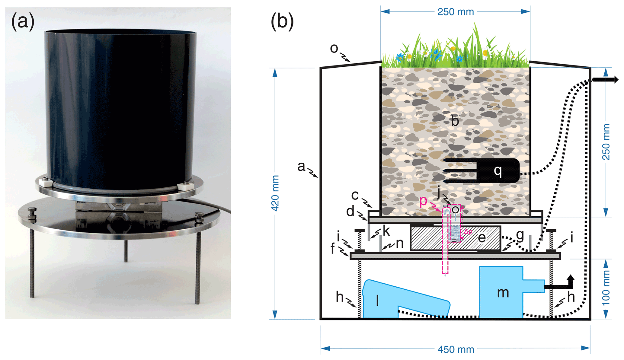
Figure 1Inner part of the ML (a) and schematic drawing of ML design (b) with a: outer part, b: ML pot, c: socket, d: load plate, e: load cell, f: base plate, g: spacing washer, h: adjustable support feet, i: counter nut for adjustable support feet, j: drainage-water outlet, k: water guide, l: float switch, m: bilge pump, n: water and dirt protection, o: cover lid, p: optional sensor or drop counter to quantify drainage for applications that do not specifically target drought conditions, and q: soil moisture and temperature sensor.
2.2.2 Drainage-water flow
To avoid stagnating water inside of ML pots, a passive drainage-water flow path was made. The drainage water was guided away from the load cell to a reservoir to protect the load cell from suspended matter. Suspended matter can be carried along with drainage water and could impede the function of the load cell by blocking the load cell bending. Drainage water beyond soil field capacity was allowed to flow out from the bottom of the ML pot via drainage-water outlets. Three drainage-water outlets (Fig. 1b:j; 0.8 cm diameter) were drilled equidistantly into the lateral side of the ML pot as close as possible to the bottom. The drainage-water outlets were protected with a metal mesh to prevent erosion of ML soil during heavy rainfall events. Excessive water could follow a passive drainage path from the top of the load plate, guided by a water guide (Fig. 1b:k; 3 cm height, 0.4 cm thick), to the base plate. From the base plate water could flow to an approximately 10 cm-high reservoir below the base plate. If the collected water in the reservoir exceeded a certain threshold, a float switch (Fig. 1b:l; Fujian Baida Pump, Fuan, China) gave a signal to a bilge pump (Fig. 1b:m; Fujian Baida Pump, Fuan, China) that pumped the water away from the ML system (schematically shown with an arrow in Fig. 1b) via a flexible tube (2 cm inner diameter). The load cell was protected from drainage-water flow by a rectangular water and dirt protection (Fig. 1b:n, PVC XT, 25 cm×10.5 cm, 4 cm height). It was glued at the base plate around the load cell and made watertight with silicon.
Rainfall could also enter in the gap between the ML pot and the outer part of the ML system. To minimize this water collection, a cover lid (Fig. 1b:o) made of a PVC-XT ring (47 cm outer diameter, 26 cm inner diameter) was constructed. The cover lid had an inclination of 7∘ towards the outside. This was done by putting the cover lid in a heated oven at 90 ∘C and then pressing it towards a custom-made wooden fit with the desired form till it had cooled down. The slanted cover lid resulted in a preferred water flow towards the surroundings and thereby prevented water flow towards the inside of the ML system. Furthermore, it protected the ML pot from incident solar radiation, also minimizing potential heating effects. Wiring of the load cell, the float switch, the bilge pump, as well as the soil temperature and moisture sensors was bundled and led out close to the top of the outer part of the ML system (schematically shown with an arrow in Fig. 1b).
In the design as used here, i.e. to quantify NRW inputs during rain-free periods, drainage water was allowed to freely drain from the ML pots. Thus, rainfall periods had to be excluded from analysis (see Sect. 2.2.3). However, to use the ML system during and shortly after rainfall periods, it is recommended to add an additional sensor (Fig. 1b:p) to quantify drainage-water flow (see Appendix E). For applications without such an additional sensor, it should be kept in mind that, depending on soil type, up to 41.5 h after intensive rainfall that saturated the soil monolith completely, drainage-water losses can occur (see Fig. F1 and Table F1).
2.2.3 Calculation of NRW amounts and differentiation of NRW inputs
We differentiated six types of NRW events with ML and ancillary sensors, i.e. (1) dew only, (2) hoar frost only, (3) fog only, (4) rime only, (5) combined dew and fog events, and (6) combined hoar frost and rime events. During all six event types, a mass increase was expected on the ML. The NRW amounts (NRWmass) were calculated using Eq. (1):
where MLmax1m is the maximum value of the 1 min mean ML mass (all three ML values averaged every minute) over a time period of 24 h (from 12:00 to 12:00 UTC), and MLmin1m is the minimum value of the 1 min mean ML mass over the same time period. The resulting NRWmass (in grams) was then converted to millimetres. If rainfall occurred during an analysed 24 h period, that period was excluded, except when the rain event occurred directly after the NRW input event. Rain events were determined by the rain-gauge measurements at the site. Time periods with a snow cover as determined visually from digital images were not considered in the analysis. To distinguish between different types of NRW inputs, we used the information from all ancillary sensors. Often dew and fog or hoar frost and rime occurred in combination: e.g. after sunset, dew formation occurred, when the atmosphere cooled further down till the atmosphere got highly saturated, and fog started to form. We termed such events combined dew and fog events or hoar frost and rime events, respectively. The leaf wetness sensor was used to sense condensation (during dew-only and hoar-frost-only events) and NRW droplet interception and impaction (during fog, rime, combined dew and fog, and combined hoar frost and rime events) and to sense an absence of condensation (during events when less condensation is expected to occur, e.g. water vapour adsorption or dew formation on soil). The visibility sensor was used to distinguish between events with reduced visibility below 1000 m (fog, rime events) and events without reduced visibility (dew-only, hoar-frost-only events). To distinguish between fog and rime events from dew and hoar frost events, the temperature sensor of the nearby agrometeorological station was used. When temperature dropped below 0 ∘C, NRW inputs were attributed to rime and hoar frost.
2.2.4 Load cell calibration and determination of accuracy
In this study, weighing accuracy denotes the difference between the measured mass (determined with a ML) and the control (calibrated mass). Precision reflects the reliability of the measurements, and it specifies to what extent the experiment can be repeated. On the other hand, resolution is the smallest distinguishable unit for an observable change in mass and thus determines the upper limit of precision. For NRW studies, high accuracy is indispensable, which requires instruments with high resolution paired with high precision.
Calibration runs for ML and the determination of the accuracy of the measurements were performed in a laboratory with closed windows and doors to avoid any influence of turbulence on load cell readings. Raw data were filtered as described in Appendix D during load cell calibration of the ML. A two-point calibration was performed on every single ML using calibration mass. For mass increases up to 500 g, calibration masses complying with the OIML F1 standard (Mettler Toledo, Greifensee, Switzerland) were used. The maximum permissible error of these calibration masses is ±2.5 mg. For mass increases of 1000 g, custom-made masses of steel were used. Their mass was determined on a laboratory scale (XS4002S DeltaRange, Mettler Toledo, Switzerland) which was calibrated and certified for determining mass up to 4.1 kg with an accuracy of ±0.01 g. First, a zero-point calibration was carried out, and then the span was set to 15 045.2 g, as this was the approximate mass which most moist ML pots had. The offset from the zero-point calibration was used together with the span calibration value in the code running on the microcontroller. The absolute accuracy of the load cells was tested on 2 April 2019 by loading calibration mass on the weighing platform in the range of 0 to 19.5 kg. The mass was increased stepwise by 500 g. The maximum mass was set to 19.5 kg to avoid an overload damage of the load cell. Three repetitions were performed. A linear regression was performed in order to assess the relationship between target mass and load cell mass. Moreover, a relative calibration was performed on 7 April 2019. We investigated the accuracy of a load cell with relative mass changes. A base mass, ranging from 10 to 19.5 kg, was loaded on the weighing platform, and then a 100 g calibration mass was added to the base mass. Accuracy of relative mass changes was determined with three replications. To test accuracy also under field conditions, we regularly performed a loading/unloading experiment following Nolz et al. (2013) by loading 5 to 10 g calibration masses on the ML and noting the mass before and after the loading. Because masses can be calibrated with certified standards as was done here, we use the term “accuracy” in this context, which goes beyond (relative) precision.
2.2.5 Evaluation of the effects of ML size on plant growth, canopy temperatures, and soil moistures and temperatures
Plant growth in the ML system was evaluated by comparing individual plant heights in the ML pots vs. the control (surroundings). Plant heights were measured from ground level to maximum standing height. Plant heights of Trifolium pratense, Plantago major, and Rhinanthus alectorolophus were measured at CH-FRU on 26 July 2019, with three replications per species and treatment (ML pot, control). To test for a statistically significant difference between plant heights of ML pots and the control (surroundings), we used a t test (n=3). To compare canopy temperatures of ML and the control (surroundings) during a NRW input period, we used a thermal camera (testo 882, Testo AG, Lenzkirch, Germany) with a thermal sensitivity of ±0.05 ∘C. Thermal infrared images were taken from 18:27 to 05:15 UTC of ML vegetation and of the control (surroundings) at CH-FRU during a dew night on 24 to 25 June 2019. Thermal images of the control (surroundings) were taken at a distance of ca. 100 cm from the ML system to exclude any potential influences of the ML system on its immediate surroundings. To compare thermal images of the ML surface with the control, we compared the variance (F test). Data were bootstrapped to reduce sample size from >30 000 to 30 samples using the scikit-learn machine learning package of Python (Pedregosa et al., 2011). Soil moisture and temperature data of ML pots and the control (surroundings) were retrieved by soil temperature and moisture sensors (Fig. 1b:q; 5TM, Meter Group AG, Munich, Germany) installed at a soil depth of 15 cm. As a control, one additional sensor was placed outside the ML system at the same depth in the surroundings. We measured over a period from the beginning of May till mid October 2019. Soil moisture data were compared as water-filled pore space (WFPS). WFPS was used to make soil moisture values more comparable by minimizing the effects of soil texture, e.g. different gravel content, that might be present in close proximity to the sensors. Higher or lower gravel content could bias soil saturation. WFPS was calculated relative to a saturation point (100 %), which was reached when the soil was fully saturated with water after long and intensive rainfall. To test whether the difference of WFPS values of ML pots and the control (surroundings) stayed constant over time, we used a co-integration test following Engle and Granger (1987), which can be used to test for co-movement of two non-stationary variables. To test whether the WFPS time series were non-stationary, we used an augmented Dickey–Fuller (ADF) test. To perform all statistical tests, we used the Statsmodels package (Seabold and Perktold, 2010) of Python.
3.1 Accuracy of the ML system
Three replications showed an almost perfect linear correlation (R2=0.9999) between target mass and load cell mass. Target mass was retrieved from the microcontroller after data filtering (see Appendix D). Data with a resolution of 0.1 g were used (Riedl, 2021). The root mean square errors (RMSEs) for comparisons of target mass to load cell mass of three replications were 0.43, 0.47, and 0.36 g, respectively. The standard errors (SEs) of the parameter estimates of three replications were ±0.13, ±0.14, and ±0.11 g, respectively.
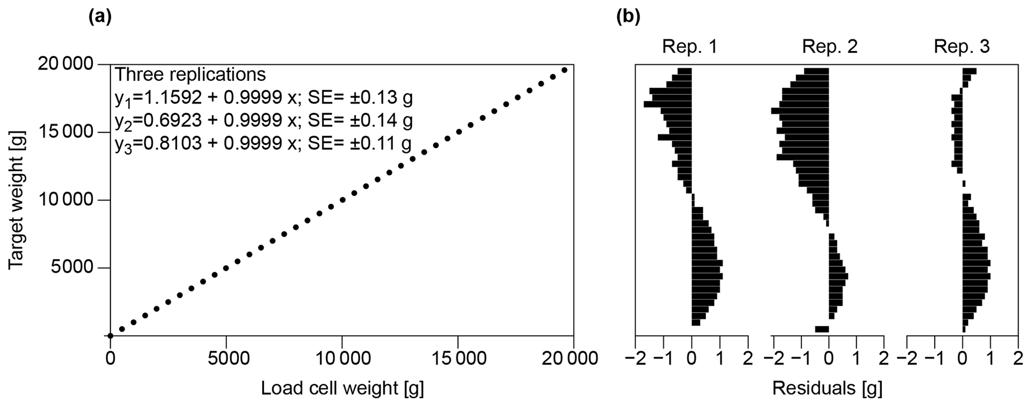
Figure 2(a) Absolute calibration of a load cell placed on a weighing platform. Three replications (overlapping data points) are shown with the SE of the intercept. (b) The residuals from the target mass of three replications (Reps. 1 to 3) were in the range of ±2 g.
NRW inputs occur during events with a finite time period, and thus for NRW input studies, the relative change in mass from the start to end of that time period is of interest. A 100 g change with the given ML size translated into a change of 2 mm water input. The residuals were in the range of ±0.25 g or ±0.005 mm equivalent water input, which represents the accuracy of the ML system (Riedl, 2021).

A zero-point offset calibration combined with data filtering (see Appendix D) gave us not only a more accurate zero-point offset, but also a more accurate span value. An accurate span value reduced fluctuating values from load cell readings and gave us stable measurements when mass changed over time. The precision was determined by repeatedly loading and unloading calibration mass on the weighing platform three times and noting the difference to test for repeatability. The precision was ±0.28 g, equivalent to ±0.005 mm water input. With a base mass over 18.5 kg, the precision was slightly lower, with ±0.45 g equivalent to ±0.009 mm water input. The digital resolution of the ML system was 0.01 g, which corresponds to 0.0002 mm equivalent water input and is thus 2 orders of magnitude better than the physical resolution provided by our ML system. Regular loading/unloading experiments following Nolz et al. (2013) showed deviations in the range between g ( mm) and ±0.4 g (±0.008 mm) and thereby confirmed high accuracy also under field conditions. Thus, the data acquisition of the ML system was accurate enough to provide high accuracy.
3.2 Differentiation among different types of NRW inputs
Our ML system allowed differentiation among different types of NRW events when the ML measurements were combined with ancillary sensors. During a combined dew and fog event (Fig. 4a), we measured an increase in mass on the ML and an increase in leaf wetness (uncalibrated sensor voltage), while visibility was partially below 1000 m (intermittent fog event). During a dew-only event, we measured an increase in mass on the ML, besides increased leaf wetness, while visibility stayed above 1000 m throughout the event (Fig. 4b). During a potential water vapour adsorption event, there was only an increase in mass on the ML, whereas no condensation occurred on the leaf wetness sensor, while the visibility stayed well above 1000 m (Fig. 4c). Wind speed remained low (<1 m s−1) during the whole potential water vapour adsorption event. Mass increases on the ML could be attributed to hoar frost if air temperature was below 0 ∘C or to rime during events with reduced horizontal visibility <1000 m and temperatures below 0 ∘C. The highest water gain of the NRW input events shown in Fig. 4 was 0.4 mm and originates from the combined dew and fog event; the water input from the dew-only event was 0.2 mm, and the lowest water input with 0.06 mm came from the potential water vapour adsorption event.
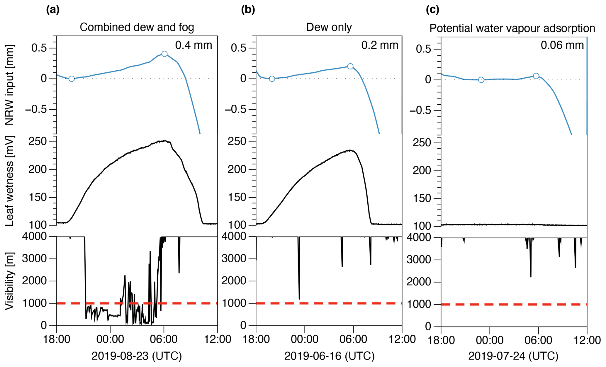
Figure 4Differentiation of different NRW input events with the ML system and ancillary sensors. (a) Combined dew and fog event. (b) Dew-only event. (c) Potential water vapour adsorption event. The black dashed line indicates the zero line. The red dashed line is the threshold for fog events with a visibility <1000 m. Visibilities >4000 m were reported as 4000 m. Blue circles indicate the start and end of NRW input events.
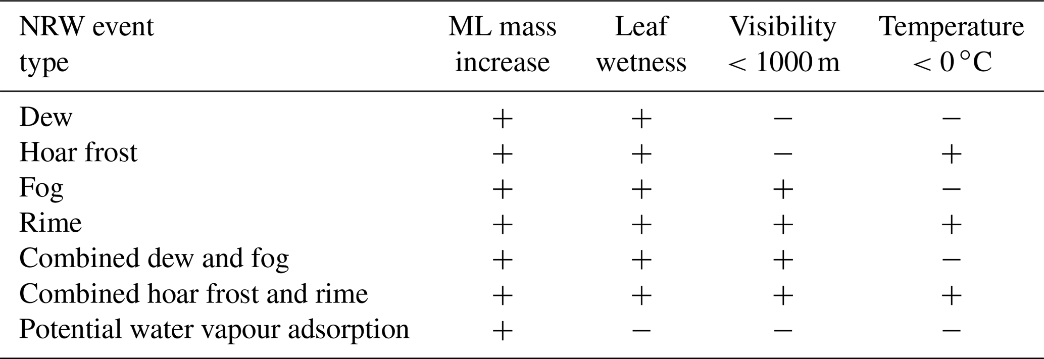
Table 1Cross table to indicate different criteria for differentiation among different NRW events. The “+” sign indicates the presence, whereas the “−” sign indicates the absence of a certain factor. All NRW events lead to increase in ML mass; ancillary sensors of leaf wetness, visibility, and temperature are needed to differentiate between NRW events.
3.3 Influence of ML system design on plant canopy temperature
Canopy temperature did not differ significantly (t test, p>0.05, n=30) between ML vegetation and control (Fig. 5a and b). The standard deviation of temperature data between the ML surface and the control was <0.5 ∘C throughout the observation period. The variance of canopy temperature between the ML vegetation and the control was not statistically significantly different (F test, p>0.05, n=30). Soil temperature in ML pot 1 was higher than in the control plot at the beginning of the dew formation period (Fig. 5c) but equalled control soil temperatures towards the end. Dew formation started at 18:53 and ended at 06:07 UTC (Fig. 5d). Dew water input was 0.24 mm, showcased for ML 1, even though dew formation occurred during that night on all three MLs installed at the site (Riedl, 2021).
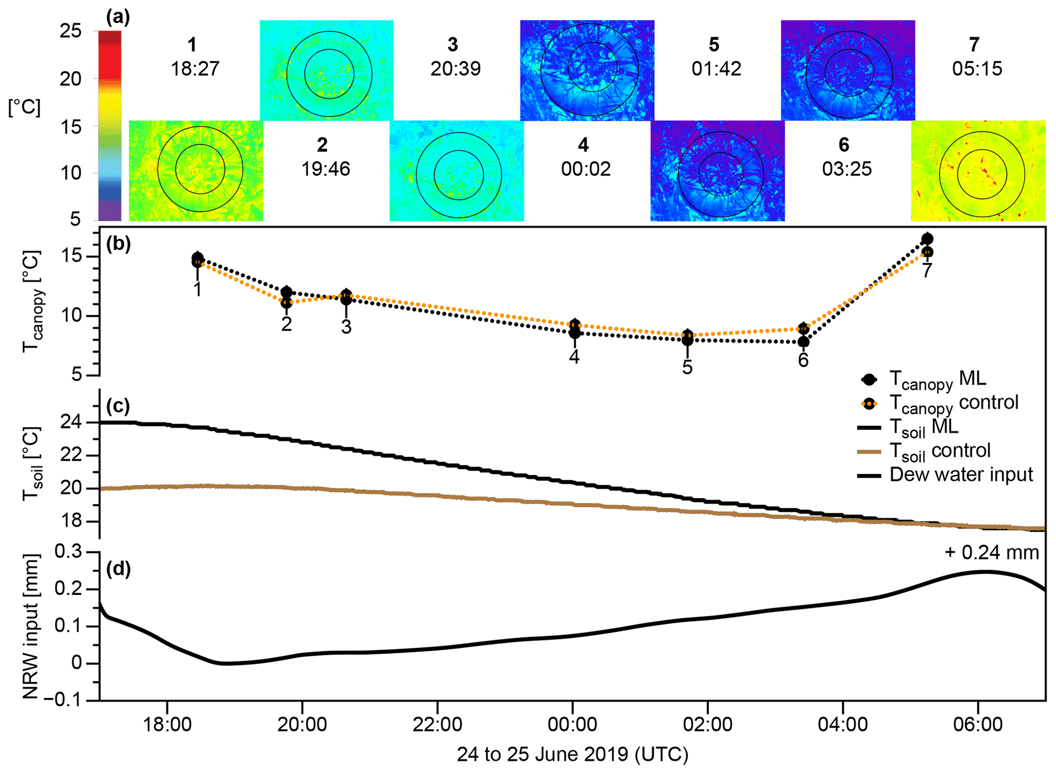
Figure 5Canopy temperatures (a, b), soil temperatures (c), and NRW input (d) of ML1 and the control (surrounding area) at CH-FRU during 24 to 25 June 2019. Time of day (HH:MM) is given in UTC time. The thermal infrared images (a) show the ML pot (small circle) with the cover lid (between the small circle and the big circle) and the surroundings (outside of the big circle) during selected time points (1–7) of a dew night. Image size is ca. 75×75 cm. To compare ML pot temperatures to temperatures of the surroundings, separate images were taken at a distance of ca. 100 cm (images not shown here) with a size of ca. 75×75 cm to exclude any potential influence of the ML on its approximate surroundings.
3.4 Influence of ML system design on plant growth
Plant heights of Trifolium pratense, Plantago major, and Rhinanthus alectorolophus did not differ between ML pots and the control (t test, p>0.05, n=3); also, variability did not differ (F test, p>0.05, n=3). Additional measurements of mean and maximum vegetation height on 14 August 2019 also showed no statistically significant difference (t test, p>0.05, n=3; data not shown; Riedl, 2021).
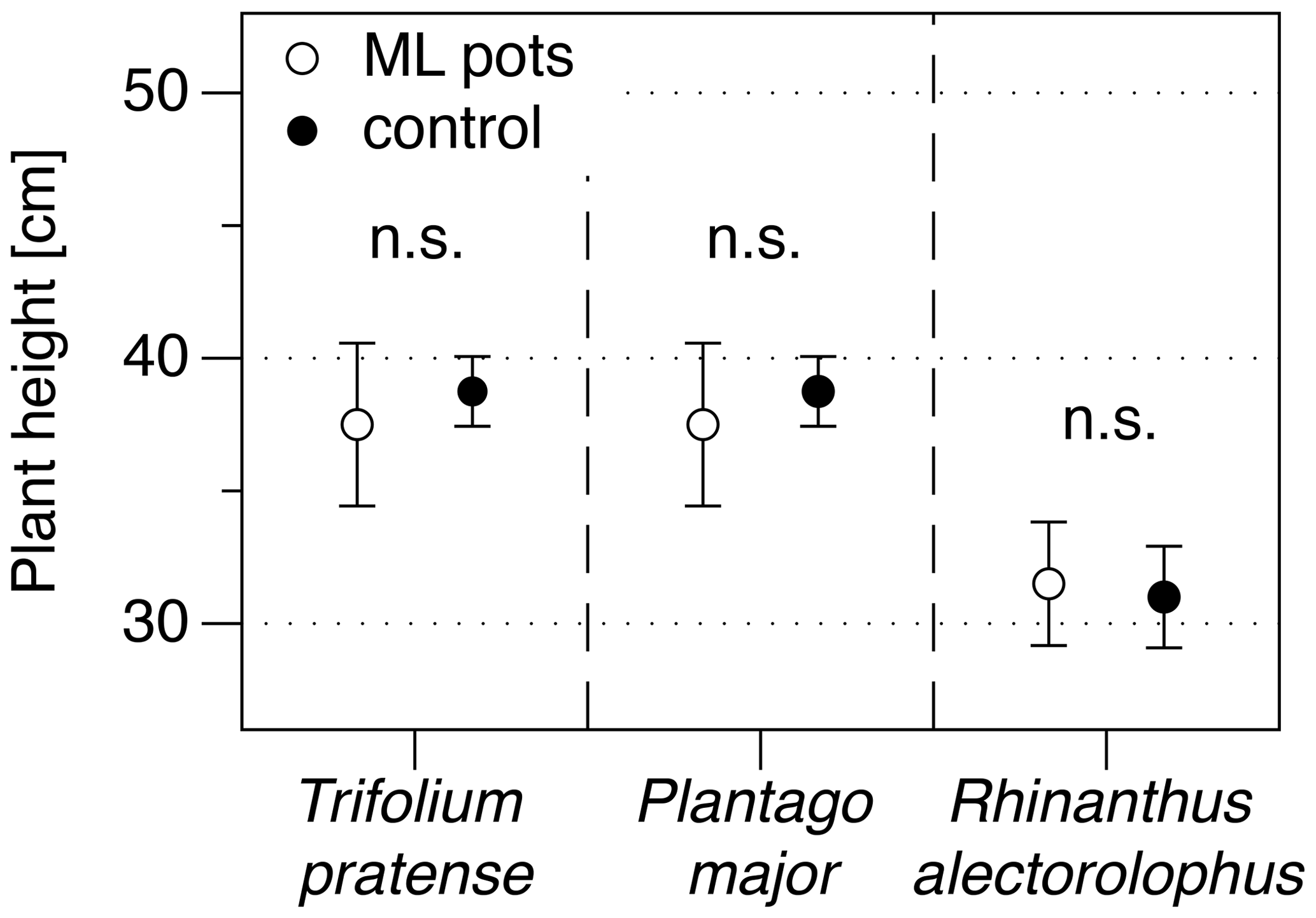
Figure 6Comparison of plant height of three plant species at CH-FRU (measured on 26 May 2019) growing in ML pots vs. the same species growing in the open field (control). Error bars show standard errors (n=3), and n.s. stands for no statistically significant difference.
3.5 Influence of ML system design on soil moistures and temperatures
WFPS data of ML pot 1 and ML pot 2 were very similar and closely matched the control (Fig. 7a). WFPS values of ML pot 3 showed a higher dynamic but closely followed the temporal pattern of the control and ML pots 1 and 2. The differences between WFPS of ML pots and the control were constant over time (Engle–Granger two-step co-integration test; p<0.05). This indicates that soil moisture data of ML pots and the control were in general not significantly different. However, during a prolonged no-rainfall period in summer (Fig. 7a, marked with the red box), WFPS of ML pots decreased more quickly in comparison to the control. Since lower soil moisture values can result in a lower heat capacity of the soil, we assessed whether lower WFPS values inside ML pots may have an influence on soil temperature during non-rainfall periods (Fig. 7b).
Soil temperature of ML pot 1 and the control (soil temperature in the surroundings) (Fig. 7b) showed the same increasing trend, while deviation of WFPS of ML pots from the control (Fig. 7a, marked in red) increased with time (the same pattern as that of ML pot 1 was also evident in ML pot 2 and ML pot 3, data not shown). From this we conclude that soil temperatures inside ML pots during the most relevant hours of the day when dew forms (during the night before sunrise) were not strongly influenced by a lower water content and its resulting lower heat capacity. Nocturnal temperature minima almost perfectly agreed between ML pot 1 and the control, while the daily temperature range of ML pot 1 was double compared to the control (Fig. 7b). Over the prolonged no-rainfall period, the hourly mean soil temperature deviations of ML pot 1 from the control ranged between −0.14 ∘C around sunrise and 2.57 ∘C in the later afternoon (Fig. 7c). Over the period from May to October 90 % of nocturnal 1 min soil temperature deviations (sunset–sunrise) were lower than 2.90 ∘C, and 50 % were lower than 0.69 ∘C.
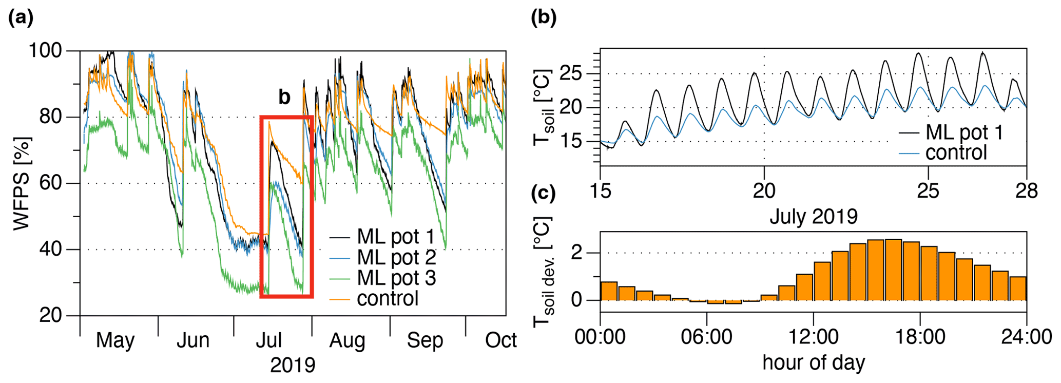
Figure 7(a) Comparison of WFPS (based on soil moisture measured at 15 cm depth) inside the ML pots vs. the control from the beginning of May till the middle of October 2019 at CH-FRU. (b) Soil temperature from ML pot 1 at CH-FRU during a non-rainfall period in July (marked with the red box in panel (a)). (c) Soil temperature deviations of ML pot 1 from the control by hour of day during the same period as marked in panel (a) and used in panel (b).
3.6 NRW inputs over 1 year
There were a total of 127 NRW input events at CH-FRU over 1 year (2 May 2019, 12:00 UTC, to 2 May 2020, 11:59 UTC; Fig. 8). The frequency of the events can be found in Table 2. Eleven NRW events were observed when leaf wetness remained low, potentially indicating water vapour adsorption events or dew formation on soil. Potential water vapour adsorption events occurred during two time periods: period 1 in July 2019 and period 2 in April 2020. During period 1, a single potential water vapour adsorption event occurred, whereas during period 2 10 such events occurred. During both periods rainfall was low: 10 d before the event in period 1 the cumulative rainfall was only 9.6 mm, and in period 2 the cumulative rainfall between 14 March, the last bigger rainfall event with 12.3 mm, and 23 April was only 13.7 mm. The soil moisture during both potential water vapour adsorption periods was rather low, with a WFPS of ca. 45 %. This indicates a potential water vapour gradient from the atmosphere to the soil favourable for water vapour adsorption. The cumulative NRW input over 12 months was 15.9 mm, which corresponds to roughly 1 % of the 1580 mm annual precipitation collected during the third-warmest year in Switzerland since weather recordings started in 1864 (MeteoSchweiz, 2020).
Table 2Number counts of events with its associated NRW input by type and percentage of the total NRW input during the observation period of 12 months at CH-FRU.
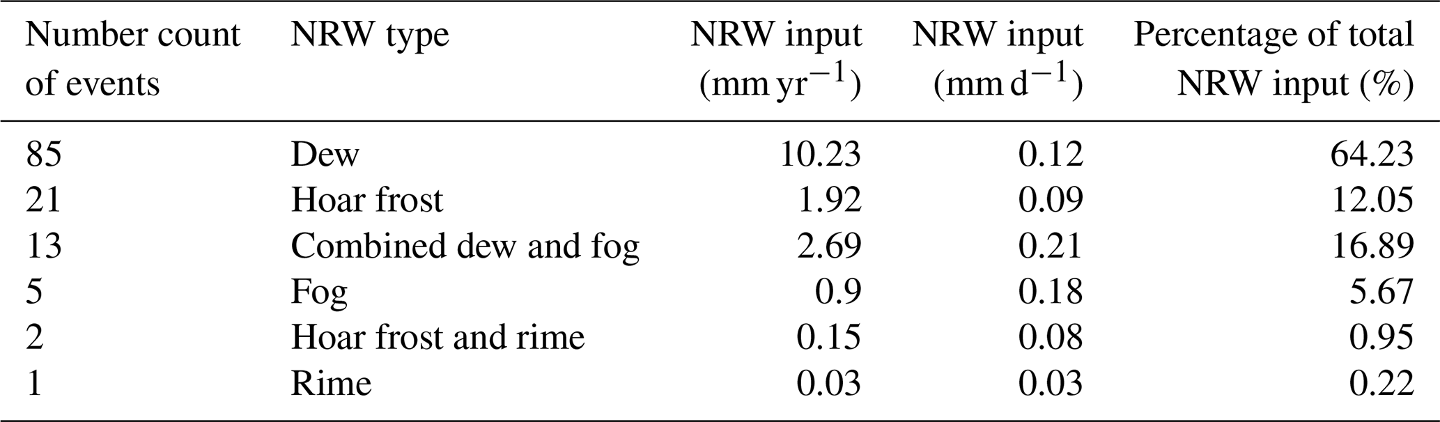
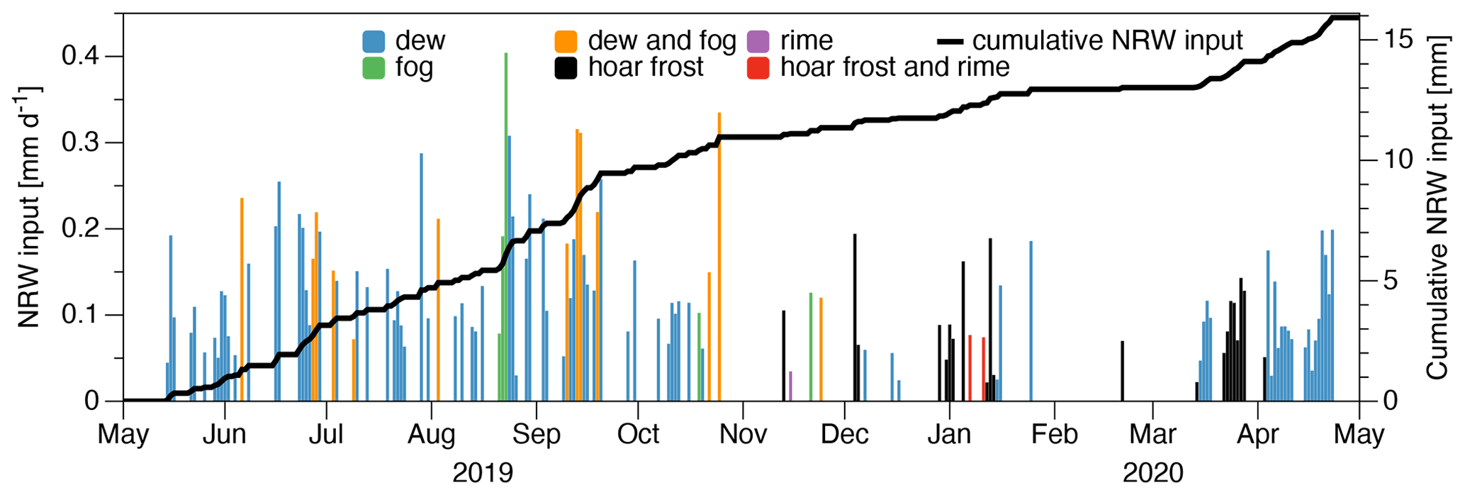
Figure 8Daily NRW inputs at CH-FRU over 1 year from 2 May 2019 till 2 May 2020. The blue bars indicate NRW events with their corresponding NRW input per day. Different colours indicate different types of NRW inputs. The black line indicates the cumulative NRW input over 1 year. The annual total NRW input was 15.9 mm, about 1 % of total precipitation during this time.
The mean NRW input over all events was 0.12 mm, with the highest single input of 0.4 mm by a fog event and the lowest input of 0.021 mm by a hoar frost event. On a monthly basis, the months with the highest NRW inputs were September with 2.64 mm, August with 2.35 mm, and June with 2.32 mm. The cumulative NRW input from May till September was 9.7 mm. At the monthly scale, NRW inputs can be remarkable: in April 2020, the month with the least rainfall (51.8 mm), the contribution of NRW input to the monthly hydrological input was 3.5 %. The average monthly NRW input was highest in September with 0.088 mm, when the nights were longer than in summer, and thus the probability of NRW inputs was increasing with the duration of the night. However, observed average monthly NRW inputs ranked second and third in terms of amount in June and August, when nights were much shorter than in September. The relationship between NRW input as a function of actual NRW input duration (Fig. 9) was not very strong, but when durations were binned into 10 bins of equal widths, a clear trend of increasing NRW inputs with increasing NRW input duration emerged. Because no NRW input is expected if the duration of NRW input is 0 h, we first started with a square-root regression through the origin, , the slope of the fit was 0.042±0.001 mm h (Fig. 9, dotted line), but for durations >2 h it closely corresponded to a conventional linear regression slope of 0.008±0.001 mm h−1 (Fig. 9, black line, R2=0.86, p<0.001; the intercept should be ignored because it has no physical meaning in this context). Despite this rather clear dependence on the actual duration of NRW input, there was no significant correlation found between average monthly NRW input duration and potential NRW input duration given by the time between sunset and sunrise (R2=0.16, p>0.1; data not shown; Riedl, 2021).
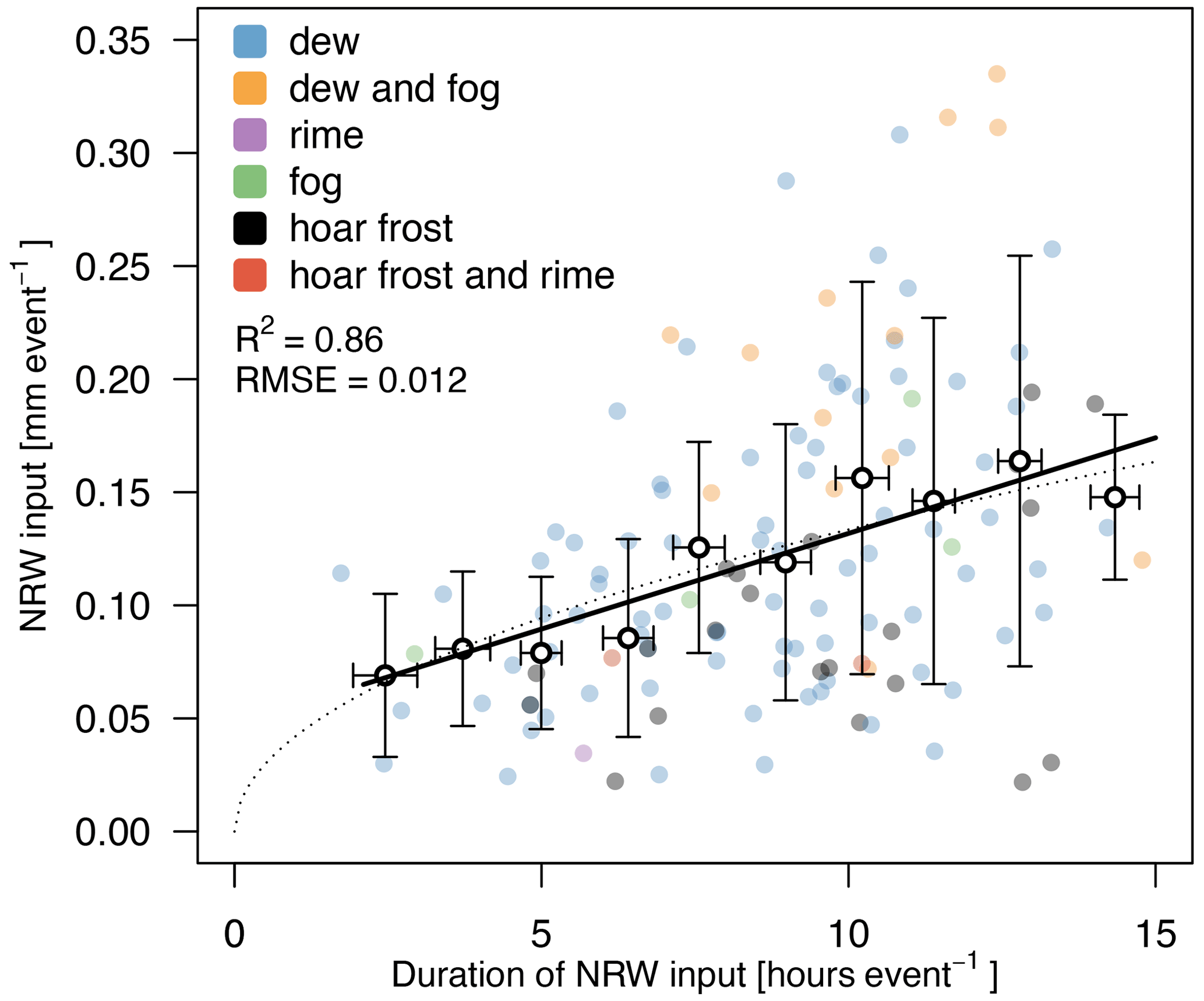
Figure 9The relationship of actual NRW input as a function of actual NRW input duration from 12 months of NRW inputs. NRW inputs were binned into 10 bins of equal width covering the entire data range of the NRW input duration. Horizontal and vertical whiskers indicate the standard deviation (SD) of the available data within each bin relative to the respective bin average (open circles). Different colours indicate different types of NRW inputs. There is a strong linear relationship (R2=0.86, p<0.001) between actual NRW input and actual NRW input duration.
4.1 Accuracy of the ML system
The high accuracy of our newly developed ML system allowed us to capture even very small NRW events such as the potential water vapour adsorption event with 0.06 mm shown in Fig. 4c. It was possible to capture NRW events with an accuracy of ±0.25 g with pots that weigh roughly 15 kg in total. This corresponds to an accuracy of ±0.005 mm of water inputs. The accuracy would be even higher with a relative mass change of less than 100 g (equivalent to 2 mm water input), which is true for most NRW events. The accuracy of our ML system was 4 orders of magnitude better than reported for many other studies (see Table 3). Feigenwinter et al. (2020) were able to achieve on average (depending on the calibration date) the same accuracy, although with a lower depth of the ML pot (6.5 cm) and a lower weighing capacity (7 kg). The high accuracy of our ML system was achieved by a combination of factors, such as using a state-of-the-art load cell in combination with continuous high-frequency data filtering as well as ancillary data. For example, temperature measurements were crucial for differentiating between hoar frost and dew events and fog and rime events. Ancillary wind measurements could be used to exclude periods with high wind speeds, because high wind could act as a force on ML and thereby increase mass. However, NRW inputs occur during conditions with low wind speed, and the probability of dew formation decreases below 5 % when wind speeds are smaller than 0.4 m s−1 or bigger than 1.9 m s−1 (Zhang et al., 2014). Thus, wind is not a big bias source for NRW quantification. A further factor promoting high accuracy was a load-cell-specific calibration. Factory calibration is the same for all load cells of the same model, but when an individual calibration is made, the differences among individual load cells are substantial, and hence the highest accuracy always requires a load-cell-specific calibration by the user. Construction details that promoted accuracy were the frictionless gap construction between ML pot and cover lid as well as the three adjustable support feet on which the weighing platform was centred on the load cell. This is needed because after burial, a ML system may accidentally tip, twist, and be thrown out of balance (Uclés et al., 2013). The low-cost microcontroller had enough computing power to continuously process data from multiple sensors while consuming little energy. Thus, our ML system could also be powered by solar panels. During or after freezing temperature conditions the ML system should be controlled, because expanding water in the reservoir or the ML pot could break PVC parts of the ML system. However, this did not occur during this study period.
The precision (repeatability of the measurements) of our ML system was ±0.005 mm equivalent water input. With a base mass over 18.5 kg, the precision was lower, with ±0.009 mm equivalent water input. However, in the field, ML pots weighed less than 18.5 kg, even when soil was moist. This precision was unprecedented, only topped by manual ML weighing on an electronic balance (Jia et al., 2014). Manual weighing is, however, very labour intensive and consequently unsuitable for long-term NRW studies.
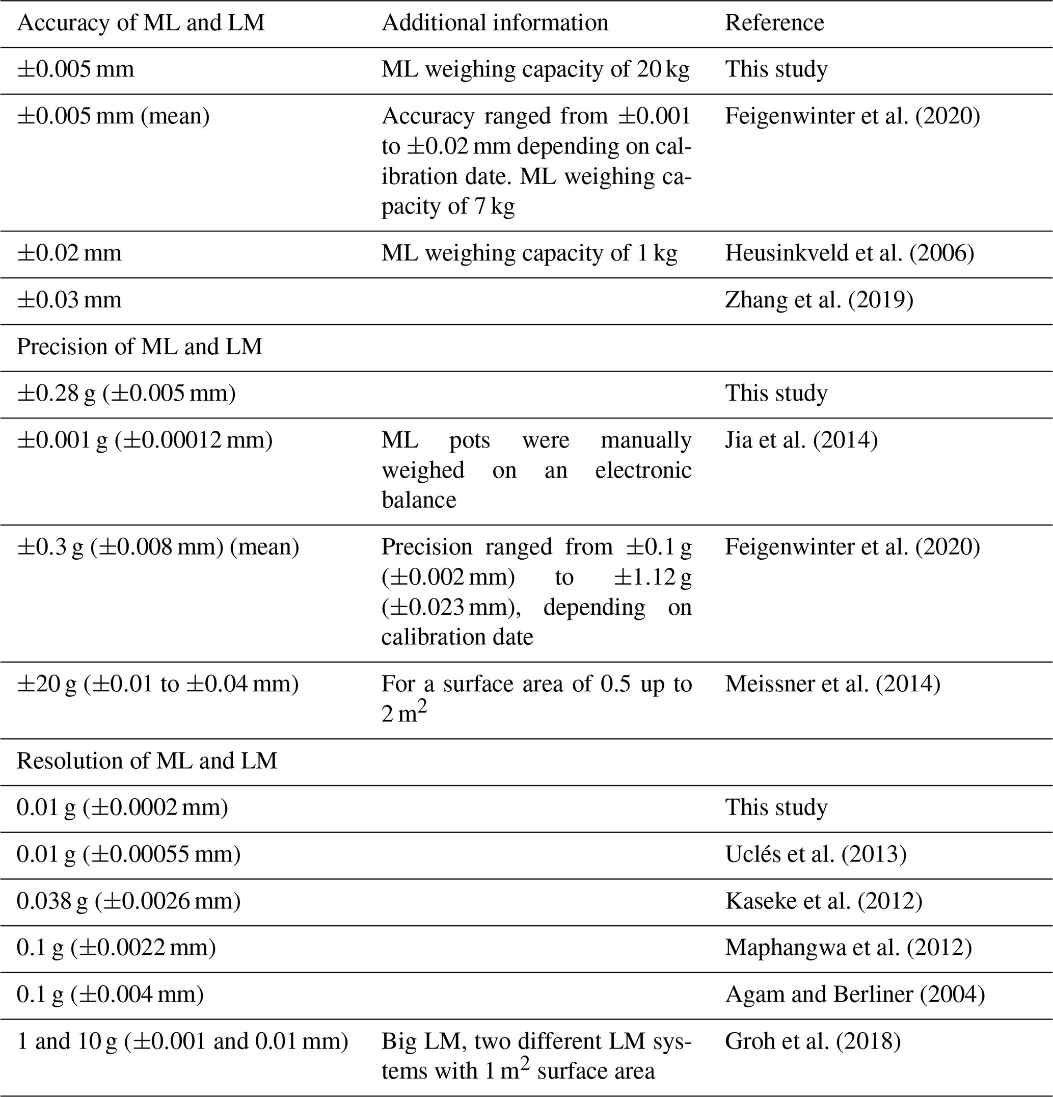
The digital resolution (smallest distinguishable unit) of our ML system was 0.0002 mm. This resolution was in the range reported by Uclés et al. (2013). Comparison of accuracies, precisions, and resolutions with other studies is often hampered, because the distinct terms “accuracy”, “precision”, and “resolution” are often misconceived. The load cell capacity of 20 kg in our ML system is relatively large compared to other ML studies. NRW input studies with ML had a load cell capacity in the range from 0.3 kg (Brown et al., 2008), 1.5 kg (Kaseke et al., 2012), 3 kg (Uclés et al., 2013), 6 kg (Maphangwa et al., 2012; Matimati et al., 2013), up to 7 kg (Feigenwinter et al., 2020).
Table 3Comparison of accuracies, precisions, and resolutions of micro-lysimeters (MLs) and lysimeters (LMs) for NRW studies.
4.2 Quantification and differentiation among different types of NRW inputs
NRW inputs occurred rather frequently over the entire year of observation (Fig. 8). NRW inputs could be measured on approximately every third day on average. The highest NRW inputs occurred during the months of main grass growth (April–September), indicating a potential hydroecological relevance. Ancillary sensors allowed differentiation of different NRW inputs. Differentiation among different types of NRW inputs is important for various research disciplines; e.g. the prediction of fog events poses a major challenge for numerical weather prediction for meteorologists (Westerhuis et al., 2020). Thus, it is important to measure the frequency and water inputs of fog events during the whole year.
The use of a visibility sensor allowed us to assess the contribution of fog and rime. A leaf wetness sensor allowed differentiation between events in which condensation occurred (dew, hoar frost), in contrast to events when condensation on leaves was less probable (water vapour adsorption and/or dew formation on soil). Potential water vapour adsorption events occurred during periods with low rainfall, when soil was drying out, which increased the vapour pressure deficit gradient between soil and the atmosphere, promoting water vapour adsorption. However, the NRW inputs of the potential water vapour adsorption events were rather low (0.03–0.13 mm). Thus, it is not unlikely that a leaf wetness sensor might react slightly differently than a true plant leaf despite the care that was taken to design leaf wetness sensors to match the radiative and thermodynamic properties of plant leaves, and these events were small dew events. Further investigations are needed to clarify whether the leaf wetness sensor is suitable for differentiating between dew and water vapour adsorption events. Air temperature measurements from the agrometeorological station were necessary to differentiate between dew vs. hoar frost formation and between fog vs. rime. Rainfall measurements allowed differentiation between NRW events and rainfall events, and a networked digital camera allowed us to observe persisting snow cover. The installation of three MLs allowed exclusion of possible effects by insects, snails, and lizards arriving on or departing from a ML pot. If it is assumed that these animals have no preference for a particular ML pot and thus their arrival and departure form a random process, such effects only contribute to the noise that is filtered out during data filtering and thus should not bias our NRW input estimates. In deserts or arid regions (with low vegetation cover), additional sensors (e.g. infrared video cameras) would be needed to detect depositing materials like dust and sand that accumulate on the ML over time. The installation of multiple MLs furthermore had the advantage that spatial variation in soils, species composition, and leaf area could be reduced in comparison to single ML deployments.
4.3 Effect of ML size on plant growth, canopy temperatures, soil moisture, and soil temperatures
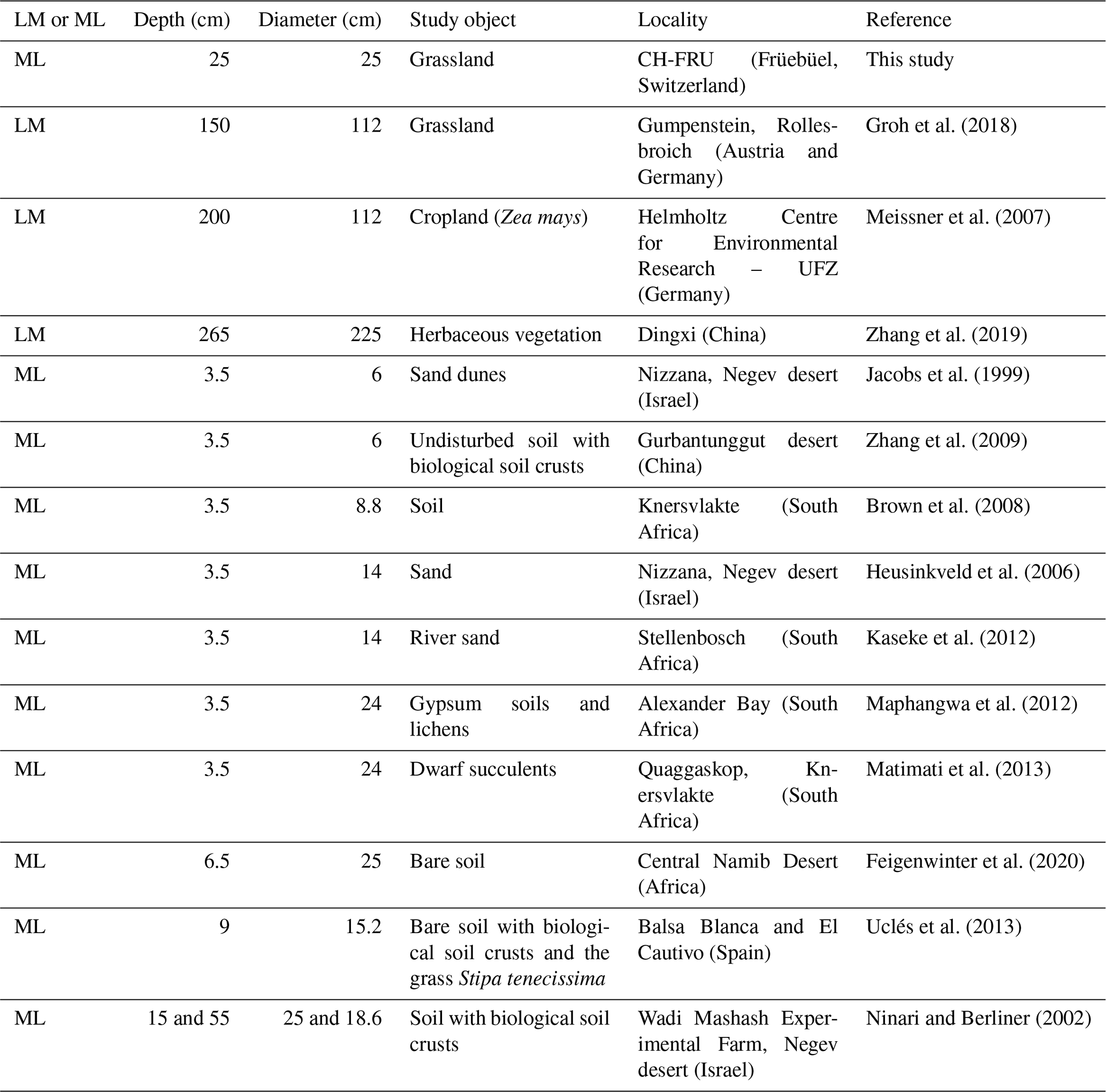
Our ML system had a larger area and a deeper ML pot than most other ML systems developed and used in earlier studies on NRW quantification (Table 4). This allowed unimpaired plant height growth (Fig. 6), representing more natural conditions than many, rather shallow ML systems, an issue crucial for accurate measurements of NRW inputs to grasses and forbs. We did not find any significant differences in canopy temperatures between our ML pots and the control (surroundings) (Fig. 5a). Furthermore, we found in general no significant difference in soil moisture between the ML and the control (surroundings); only during a prolonged drought period did soil moisture values of ML pots decrease more quickly. In this study, this however had no influence on plant standing height because measurements of plant height (before the drought period) and measurement of overall vegetation height (after the drought period) were not statistically different. However, lower soil moisture during prolonged drought periods can result in reduced evaporation rates and increased water vapour adsorption rates. Furthermore, this can influence plant growth and development. Thus, the ML system can be used to reliably measure NRW inputs as long as the difference in soil moisture during prolonged drought periods does not influence plant height or canopy architecture. WFPS values of ML pots were in general not higher than the control, suggesting a sufficient drainage by the drainage-water outlets. This is crucial, because saturation at the bottom of a ML could lead to oxygen limitation for root growth (Ben-Gal and Shani, 2002). In contrast to Kidron and Kronenfeld (2017), Evett et al. (1995), and Ninari and Berliner (2002), we also did not observe substantially lower nocturnal soil temperatures, the time when NRW inputs actually take place, which is important for avoiding an overestimation of dew formation on soils. On the other hand, afternoon and close-to-sunset soil temperatures of ML pots were higher compared to those in the control (Fig. 7). Thus, potentially, the ML system could underestimate dew formation on soils shortly after sunset, but dew formation on soils is rare (Agam and Berliner, 2004; Ninari and Berliner, 2002) and the open soil surface in grasslands is rather small, ideally zero under good management practices. Higher soil temperatures could underestimate water vapour adsorption, because it lowers the vapour pressure deficit between soil and atmosphere. Therefore, our estimates of NRW inputs on soils should be conservative estimates, given that the slightly elevated temperatures actually do reduce (not increase) NRW inputs on soil inside the ML pots. The higher soil temperatures in the afternoon were not related to a lower water content nor its associated heat capacity. Kidron et al. (2016) provided a possible explanation for the diurnal temperature difference between a ML pot and the control. They termed it a “loose stone effect”: the ML pot might act as a loose stone, i.e. through the air gap between the ML pot and the outer part of the ML system more efficient longwave radiational cooling can occur in comparison to the bulk soil. However, Ninari and Berliner (2002) found that the lateral soil temperature gradient was small compared to the vertical soil temperature gradient and that wrapping the ML pots with insulation material did not reduce temperature deviations. We thus think that insufficient ML pot depth has most likely caused the soil temperature alterations observed mainly during day-time when dew formation is absent. Ninari and Berliner (2002) suggested that the minimum ML depth should be the depth at which the temperature is constant during the entire day. For a dry loess soil in the Negev desert, a sufficient ML pot depth would be 50 cm (Ninari and Berliner, 2002). At CH-FRU, a ML pot depth of approximately 95 cm would be necessary in order to have soil temperature gradients over 24 h periods <0.5 ∘C. With a depth of 95 cm, there would be the risk that all the advantages any ML system entails would be lost. Although constructing deeper ML pots would be possible, even with double or triple the current ML pot depth, deeper ML pots would exert more dead mass onto the load cell and would thus decrease load cell accuracy (Kaseke et al., 2012). Overall, ML design is always a trade-off between representing the surroundings and feasibility of construction and installation. The ML system was not constructed with the depth suggested by Ninari and Berliner (2002); however, the aim of this study was to measure NRW inputs to grasslands, for which canopy temperatures are more important. We found only a small difference in canopy temperature between the ML and the control. Thus, we conclude that our novel ML design is suitable for quantifying nocturnal NRW inputs on grasses and forbs reliably and accurately at high temporal resolution.
Table 4Size comparison of LMs and MLs developed and used for NRW studies.
4.4 NRW inputs at CH-FRU
NRW inputs occurred on approximately one-third of the nights and were thus a frequent water input. The NRW inputs measured by our ML system represent conservative estimates under certain conditions, because drainage-water flow from the ML pots was not measured. Under conditions with water lost via drainage, NRW inputs would be underestimated. Especially during and shortly after intensive rainfall periods, when drainage-water flow is more likely (see Appendix F, Fig. F1, and Table F1), the application of the ML system is limited. During transition periods, shortly after rainfall, e.g. during nights when the sky clears after rainfall, NRW inputs may be underestimated. Therefore, we excluded such periods (see Eq. 1) from the analysis and limited our analysis for dry periods. Our longer-term NRW estimates might thus be conservative estimates if rainfall periods are included in the total hydrological input. At our site, drainage-water flow from the ML pots reached low levels rather quickly after rainfall events (see Appendices E and F for more details). Nevertheless, depending on soil characteristics and conditions, drainage-water flow could persist for a longer time (Fig. F1 and Table F1). Under such conditions, the ML system provides conservative estimates of NRW inputs, because we set NRW input to 0 mm when there is rainfall and/or drainage flow percolating out of the soil monolith. A possible modification of the ML system to also quantify such drainage flow accurately is suggested in Appendix E, with an additional sensor as indicated in Fig. 1b:p. We used three outlets (Fig. 1b:j) to ascertain that drainage is not hindered, but if a sensor to quantify drainage is added, the ML pot should only have one drainage hole with a sensor, from which reliable quantitative estimates of drainage losses can be obtained.
NRW inputs were especially high under conditions when rainfall was absent, e.g. in April, the month with the lowest rainfall. NRW inputs were not influenced by potential NRW input duration, and thus there was also a high probability of NRW inputs occurring during summer months, the main growth period of temperate grasses and forbs. In fact, the monthly average NRW inputs were similar to the NRW inputs that were measured in spring and autumn months, when NRW inputs are expected to be highest. This indicates a high ecohydrological relevance of NRW inputs for temperate grassland ecosystems, especially during hot and dry periods. However, the effects of these frequent NRW inputs on plant–water status still have to be investigated.
Besides studying the effects of NRW inputs on temperate grassland species during hot days with low soil moisture, a special focus should be directed to the effects of NRW inputs during periods with high soil moisture, when no soil water stress is present. NRW inputs could be beneficial even under such conditions, when simultaneously atmospheric demand is high (high energy input, high vapour pressure deficit). NRW inputs could reduce leaf temperatures by the re-evaporative cooling effect and thereby reduce water stress during early morning hours and consequently increase productivity (Dawson and Goldsmith, 2018). However, leaf wetting by NRW inputs could also be disadvantageous during periods with no soil water stress. Leaves covered by water droplets from NRW inputs could show reduced gas exchange due to lower gas diffusivity through the water layer. Thus, the development of the ML system and measurement of NRW inputs with high accuracy are crucial steps to address ecohydrological processes, but further investigations are necessary to understand physiological effects on grasslands.
The aim of this study was to develop a high-accuracy ML system for the quantification of NRW inputs that overcomes existing drawbacks. The ML system comprised a comparatively large and deep ML pot in the size class of 25 cm diameter ×25 cm depth in combination with an unprecedented weighing accuracy. This ML size allowed natural plant growth, and such a ML system can therefore be used in different ecosystems with most short- to mid-sized statured grasses and forbs or similar vegetation up to ca. 40 cm. Ancillary sensors allowed differentiation among different types of NRW inputs. Our study shows that the ML system represents natural conditions very well. The plant height was not significantly different between ML pots and the control (surroundings). Plant canopy temperatures of ML pots were close to canopy temperatures of the surroundings during a nocturnal period when NRW input took place. However, additional continuous canopy temperature measurements in follow-up studies could allow us to more clearly distinguish dew formation from water vapour adsorption and to identify whether canopy temperature drops below dew-point temperature. If this is not the case and other factors like rainfall and fog can be excluded, a weight increase might then be related to water vapour adsorption. Furthermore, canopy temperature measurements would clarify whether a leaf wetness sensor alone is sufficient to distinguish between dew and water vapour adsorption events. Soil temperatures were higher in ML pots, especially during the day. This could influence the hydraulic characteristics of soil water and the heat balance of the soil and in consequence lead to biased latent and sensible heat fluxes. Thus, further ML studies should primarily focus on getting rid of soil temperature differences between ML pots and the surrounding soil. In addition, the ML system could be further improved by adding water flow or water droplet sensors at the ML pot outlets to measure drainage-water flow (see Appendix E), with the goal of avoiding underestimation of NRW inputs shortly after intensive rainfall events or during soil conditions when drainage-water flow persists for a longer time (see Appendix F). With our ML system, we were able to resolve mass changes on a 15 kg pot with an accuracy of ±0.25 g, which corresponds to ±0.005 mm of water input. This accuracy allows determination of typical water gains by dew, hoar frost, fog, rime, or water vapour adsorption of the order of 0.021 to 0.4 mm in a single night. The study revealed that NRW inputs occurred frequently and provided an average of all NRW events of 0.12 mm of water. Such quantitative estimates will be essential for assessing the role that NRW inputs might have in temperate grasslands during summer drought conditions. However, longer-term NRW input measurements would allow us to see whether the seasonal patterns of NRW inputs are constant over time or whether they are influenced by weather conditions and thus vary from season to season. Moreover, the effects of NRW inputs on plant physiology in grassland ecosystems still have to be elucidated more carefully to assess the importance of such water inputs during ongoing climate change such as projected prolonged heat periods in the months of main vegetation growth.
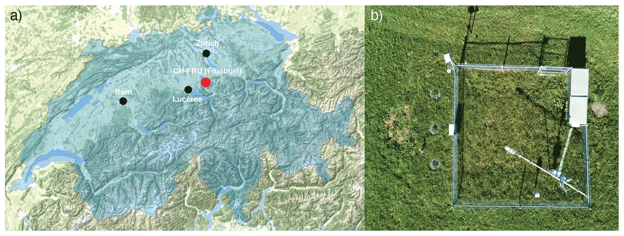
Figure A1(a) The red dot indicates the location of the CH-FRU site within the Swiss borders (blue). The black dots indicate the cities of Zurich, Bern, and Lucerne. Map tiles by © Stamen Design, under CC BY 3.0. Data by © OpenStreetMap, under ODbL. (b) Aerial photograph taken with a drone of the CH-FRU site. On the left of the fenced area the three MLs are visible.
To retrieve an undisturbed soil monolith with intact grass vegetation, we used an empty ML pot that was placed upside down at the place of interest from where the monolith was to be retrieved. First, we trenched the soil with a long spade around the ML pot. Then we removed the soil around the ML pot with small shovels, which allowed the ML pot to be pressed into the soil. We continued until the top of the ML pot was at ground level. Finally, the contact with the soil could be cut at the bottom with a spade. The reversed soil monolith was carefully taken out from the ML pot, and three people collaborated to transfer it to a second ML pot to be upright again. The ML pot was then ready for installation on the weighing platform. The weighing platform was levelled out by adjusting the three adjustable standing feet with a prolonged hexagon socket wrench. The final position was fixed with the counter nut by using an open-end wrench.
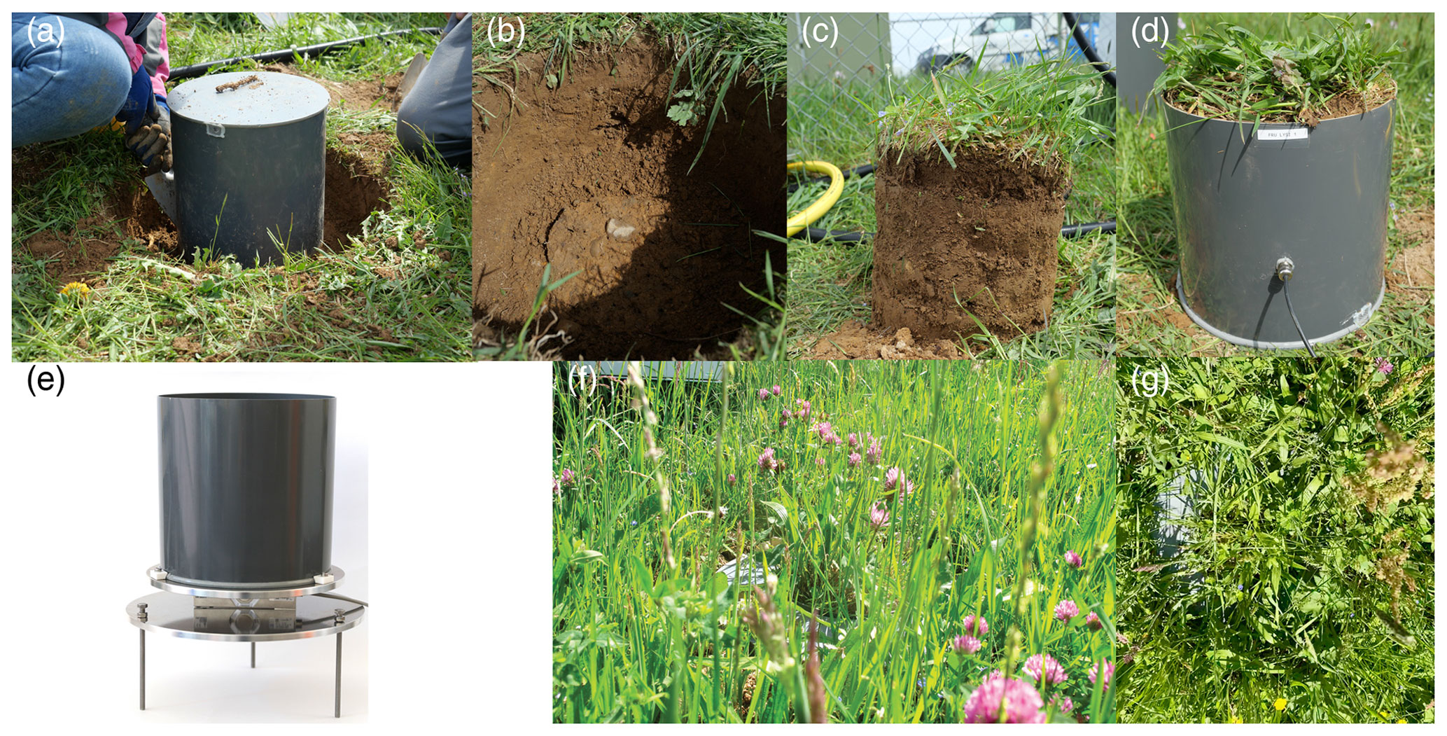
Figure B1Photographs of single ML pots during (a–e) and after (f–g) installation at CH-FRU. (a) First step to retrieve an undisturbed soil monolith. An empty ML pot was placed upside down, and then the soil around the ML pot was removed with small shovels. Afterwards the ML pot was gently pressed into the soil. (b) The contact of the monolith with the soil was cut at the bottom with a spade. (c) The monolith was removed from the ML pot and carefully transferred to a second ML pot. (d) Monolith ready for installation at the weighing platform. (e) Empty ML pot on a weighing platform. The weighing platform is standing on the adjustable support feet. (f) Lateral view of an installed ML. (g) Top view of an installed ML.
Data from all sensors were collected by an Arduino-type MEGA 2560 PRO microcontroller (RobotDyn, Zhuhai, China), which was installed on a custom-made printed circuit board (PCB). The voltage signal coming from the load cells was digitized by a 24-bit analogue-to-digital converter for weigh scales (LM711, SparkFun Electronics, Niwot, USA). For each load cell, a separate analogue-to-digital converter was used. After collecting and processing the data of the load cells and the other sensors, the data were stored as 1 min averages on a micro-SD card (MicroSD 16 GB, Kingston Technology Company Inc., Fountain Valley, USA) inserted into the slot of a micro-SD breakout board (MicroSD card breakout board 254, Adafruit Industries, New York, USA). Then, the data were transferred to our data server every 5 min by using Internet of things (IoT) technology. To send the data, a breakout board (RFM9X LoRa Radio, Adafruit Industries, New York, USA) connected to the open TheThingsNetwork was used. TheThingsNetwork uses a long-range wide-area network (LoRaWAN) protocol. A real-time clock (DS3231 for PI, HiLetgo, Shenzhen, China) was installed on the PCB to obtain exact timestamps.
Load cell data are prone to noise. To cancel the noise related to temperature fluctuations, the load cells used four strain gauges in a Wheatstone bridge configuration. Thus, noise visible in the data mostly originated from electrical noise, fluctuations in wind speed, and atmospheric pressure. To minimize this noise, we used a data-filtering algorithm on the microcontroller. The microcontroller measured the load cells nominally at 3.3 Hz in combination with the retrieval of measurements from other sensors. The raw load cell data were then stored in an averaging window (ring memory) with a size of 100 values, where the oldest values were replaced by the newest ones. The upper and lower 15 % of these values within the averaging window were discarded, and the remaining values were averaged. From the low-pass-filtered signal, 1 min means were stored on the micro-SD card. For data delivery via IoT, these mean values were further averaged over 5 min intervals to comply with the allowed IoT bandwidth for data transfers.
The ML pots were designed to avoid stagnation of water that potentially could impede plant growth by creating anaerobic conditions in the rooting zone. For that reason, a passive drainage-water flow path allowed drainage of excess water beyond field capacity. However, to further develop this ML system and use it during and shortly after rainfall periods or to improve the measurements during other periods when the soil cannot hold excessive water, it is recommended to quantify drainage-water flow. This is because NRW inputs increase the mass of ML pots, whereas drainage-water flow out of the ML pots reduces their mass. Therefore, if drainage-water flow during NRW inputs is non-zero, this would lead to an underestimation of the NRW inputs as long as no additional sensor is added to the ML pots to quantify this drainage flow.
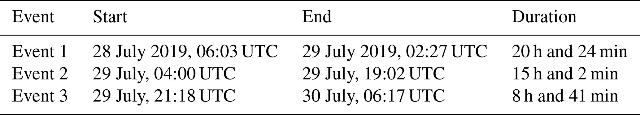
To assess the required specification of such an additional sensor and to quantify how long drainage-water flow of the ML system persists, we investigated three consecutive events (see Table E1):
-
a high-intensity, high-amount, and high-duration rainfall event (Fig. E1a, event 1),
-
an evapotranspiration event from sunrise till sunset (Fig. E1a, event 2), and
-
a NRW input event (Fig. E1a, event 3).
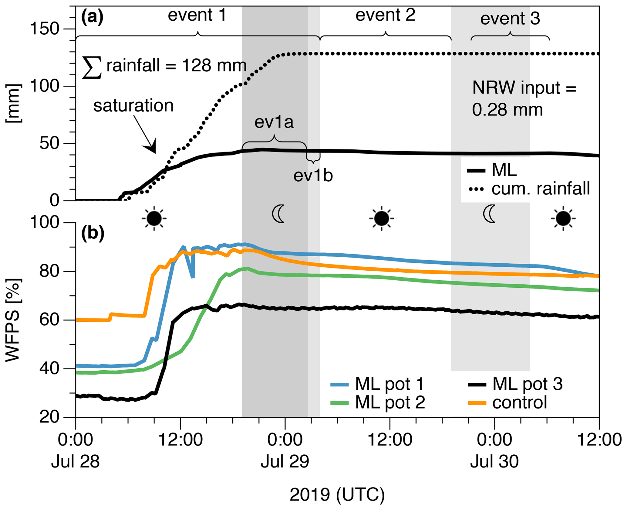
Figure E1(a) Cumulative rainfall and ML mass during a rainfall (event 1), an evapotranspiration (event 2), and a NRW (event 3) event, from 28 July, 00:00, till 30 July, 12:00 UTC. The grey-shaded areas indicate night-time duration (sunset till sunrise), the unshaded areas day-time duration (sunrise till sunset). The ML mass and the cumulative rainfall increased at the same rate until the ML pots were almost saturated (indicated with an arrow). Afterwards there was more drainage water lost from the ML pots than water gained. During the ev1a period (from sunset till the end of rainfall in event1), a rainfall water input of 26.9 mm was observed, but the ML system showed a water gain of only 0.3 mm, and the difference between the two measurements corresponds to the (unmeasured) loss via drainage-water flow. During the ev1b period (from the end of rainfall till sunrise in event1), there was no rainfall water input, but the ML system showed a water loss of 0.07 mm. During event 2 there was a water loss by evapotranspiration of 2.25 mm. During event 3 (the following night), there was no water loss but instead a water gain by NRW input of 0.28 mm. (b) WFPS inside the ML pots and the control, measured at a depth of 15 cm. WFPS reached high values after the rainfall event.
Table E1Start, end, and duration of the three events used to assess the duration of drainage-water flow from ML pots and the specification of a drainage-water flow sensor.
During event 1, the total amount of rainfall was 128.5 mm. The highest hourly rainfall intensity occurred on 28 July 2019 at 10:00 UTC with 16.8 mm h−1, which is classified as “heavy rain” >4 mm h−1 (Met Office, 2012). ML mass increased as soon as the rainfall event started and increased at the same rate during the rainfall input till ca. 11:00 UTC. Afterwards the rate of ML mass change, i.e. the slope of the ML mass increase, flattened compared to the cumulative curve of rainfall input: from the beginning of the rainfall event till sunset, the water input was 101.6 mm, whereas the ML system showed an increase of only 36.2 mm. The difference of 65.4 mm most likely corresponds to the losses from drainage-water flow because of soil saturation during such high-intensity rainfall with excessive water being lost. However, WFPS did not reach the 100 % mark (Fig. E1b). Note that the 100 % WFPS reference was determined from the full year of measurements and is thus relative to spring conditions. Therefore, it is not surprising that this mark was never reached during dry summers, even after heavy precipitation. During such a high-rainfall water input, drainage-water flow of the ML system was of the order of 64 % of the rainfall amount. However, water might not only be lost via drainage water flow but also by evapotranspiration during day-time. To quantify solely drainage water loss, the night-time period (when no evapotranspiration is expected) was further investigated. We separated the night-time period into period ev1a, when rainfall occurred, and period ev1b, when no rainfall occurred (Fig. E1a, grey-shaded periods).
During the ev1a period (Fig. E1a, period ev1a), from sunset till the end of the rainfall event, the water input was 26.9 mm, whereas the ML system showed only an increase of 0.3 mm. The difference of 26.6 mm (98 %) might be caused by losses from drainage-water flow. The water loss rate was 3.6 mm h−1. The 34 % higher drainage water loss compared to the day-time period might be due to the lower water holding capacity of the more saturated soil. During the ev1b period, starting after the ev1a period till sunrise (Fig. E1a, period ev1b), no further water gains and losses were expected, because evapotranspiration was absent during nocturnal conditions with low average wind speed (<0.6 m s−1). During period ev1b, the ML system showed a water loss of 0.07 mm, which corresponds to an average water loss of 0.05 mm h−1. This water loss can clearly be attributed to drainage-water flow. The rate of drainage-water loss was however strongly reduced (by 98 %) compared to the ev1a period. Thus, drainage-water flow of the ML system reached very low values within only 1 h and 33 min after this extraordinarily high rainfall, showing that even the current ML system can handle high drainage-water flows well.
During event 2 with no rain but evapotranspiration, the ML system indicated a water loss of 2.25 mm, which corresponds to an average evapotranspiration rate of 0.15 mm h−1. Potentially a drainage-water loss could have occurred in the morning hours on 29 July. However, the drainage-water loss most likely was <0.05 mm h−1, similar to the drainage-water flow rate during the ev1b period, just before event 2, shortly after the rainfall event. Since no new rain fell, we expect the drainage-water flow rate to decrease with time. In fact, 1 h before sunset, a further reduced ML mass loss of only 0.005 mm h−1 was recorded. This very low water loss can be attributed either to drainage-water loss or to evapotranspiration as it occurred during day-time. We conclude that the drainage-water loss could at maximum be 0.005 mm h−1 but was most likely lower due to concurrent evapotranspiration. Thus, the ML system readings were no longer significantly affected by potential drainage-water flow after only 15 h after rainfall.
During event 3, a very large dew event of 0.28 mm occurred, which was above the 95th percentile of all NRW events during the 12-month period considered in this study. Such a large dew event is unlikely to be recorded under conditions when at the same time a large drainage-water flow would also have occurred. If this had happened, the dew water input should have been lower. Thus, it is very unlikely that drainage-water flow still occurred during that dew event.
Overall, these three events showed that drainage flow occurred under rainfall conditions and shortly after rainfall events. The current ML system handled large drainage flows well and effectively; i.e. water drained quickly, avoiding long-lasting “memory” effects. Drainage flow was lower than 0.005 mm h−1 1 h before sunset during event 2, only 15 h after the last rainfall. However, at other sites with different soil characteristics, different drainage flow patterns might occur (see Appendix F), and our ML system might therefore provide conservative NRW inputs and accentuated evapotranspiration rates. If the current ML system were to be used for high-rainfall conditions, potential drainage-water flow needs to be quantified using additional sensors. Without such additional sensors, NRW inputs could be underestimated if the NRW input occurs shortly after a rainfall event and drainage-water flow indeed occurs. Consequently, the current ML system is expected to give conservative estimates of NRW inputs, especially if NRW inputs happen directly after a rainfall event.
Potential approaches to quantify the small amounts of drainage flow from a ML system are by installing a water flow sensor or a drip counter at the ML pot drainage-water outlets. The maximum rainfall intensity reported above was 16.8 mm h−1. With a ML pot diameter of 25 cm (see Sect. 2.2.1 of the main text) and the extreme assumption that 100 % of precipitation contributes to drainage-water flow, such an addition must be able to process 13.7 mL min−1. If the maximum drainage-water flow is however only expected to be <15 % of precipitation, then a sensor capable of measuring up to 2000 µL min−1 would be an adequate choice.
We recommend using a water flow sensor or a drip counter. One option is a liquid flow sensor (SLF3S-0600F, Sensirion AG, Staefa, Switzerland) that is capable of detecting low flow rates of up to ±2000 µL min−1. A drip counter can be constructed with two gold electrodes attached to the ML pots' drainage-water holes with a small gap. If a water droplet passes the gap, an electric circuit is closed which can be counted as a water drop by a data logger (Meter Group AG, 2020). Calibration of a drip counter is recommended for accurate measurements of drainage-water amount. Sensors measuring drainage-water flow would allow us to correct for drainage-water outflow and would thereby increase the usability of the current ML system for times during and shortly after rainfall events.
Drainage-water flow was not quantified in the application of the ML system described here, because the goal was to quantify NRW inputs during dry conditions without saturated soils. To estimate the duration of drainage-water flow from the bottom of the ML pot, we used the approach by Zhan et al. (2016) with modifications following Freeze and Cherry (1979) and model input parameters from Rawls et al. (1991) listed in Table F1. The full equation set used here is provided in what follows.
The relation between the unsaturated hydraulic conductivity k, the volumetric water content θ, and the porewater pressure head ψ (matrix potential) can be described by the following formula:
where γ is the slope angle (0∘ with our ML), z∗ is the axis perpendicular to the slope, and t is time. Note that we are only considering the case where ψ<ψae. In the case where ψ≥ψae, both variables kθ are constant.
In order to solve this equation, we can substitute and
and use the product rule
to get
To solve this numerically, we assume a uniform saturated ground at t=0 given by and for all z∗.
Moreover, we impose the boundary conditions at and at the top , where q is the rainfall intensity. Here we choose q=0 to look at the situation after long rainfall events.
We simulated the drying of the 25 cm-deep soil monolith using a finite-difference approach with m and Δt=10 min. The procedure carried out at each timestep was (1) to compute the drainage-water loss across the bottom of the soil monolith Per using Zhan et al.'s (2016) equation,
where k′ is the dimensionless ratio of the unsaturated hydraulic conductivity normalized by its value at saturation (ks), , and γ is the slope angle. For the simulations we assumed γ=0∘; thus, in case of a sloping surface, the drying of the soil monolith takes less time (td) than what we present in Fig. F1.
(2) This amount of water was removed from the lowest soil layer ). (3) Then the updated soil water content profile θ(z∗) was converted to an updated pressure head profile ψ (z∗) using the relationship in Eq. (F2) solved for ψ,
(4) Then the drainage flow rate for all soil layers was computed with Eq. (F5), and the respective amount was transferred from each layer to its lower adjacent layer. (5) Then the θ(z∗) profile was converted to ψ(z∗) and the change over time from Eq. (F3) was added, and then the θ(z∗) profile was updated accordingly before the next timestep was simulated.
The threshold for the end of the drainage period was set to one drop of water per day percolating out of the soil monolith's bottom (0.05 mm d−1, or 0.35 µm at the Δt=10 min timestep).
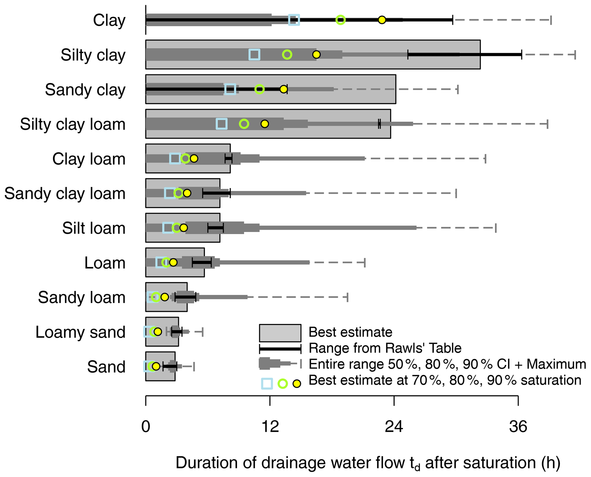
Figure F1Estimated duration of percolation (td) at the bottom of a 25 cm soil monolith in a ML for various soil types. Bars show the best estimate for each soil type for completely saturated soils, and whiskers show the range that results when the parameter range given by Rawls et al. (1991) in Table F1 is used. Symbols show the reduced td when the average water content of the soil monolith is 90 % of its saturation (yellow circles), 80 % (green circles), or 70 % (blueish circles). Because the system is highly non-linear, the parameters given in Table F1 do not result in the full range of td, and hence we added the maximum that can be obtained with intermediate model parameters for each soil type (dashed whiskers) and the 70 %, 80 %, and 90 % two-sided confidence intervals (grey bars of varying width; see legend) for all td resulting from combinations of parameter values within the bandwidth given in Table F1.
Following Timlin et al. (2004) we used the Brooks–Corey pore size distribution λ tabulated in Table F1 in combination with the effective porosity ϕe (m3 m−3) defined as the difference between total porosity ϕ (m3 m−3) minus the water retained in the soil matrix at a suction pressure of −33 kPa (θ33; m3 m−3), ,
The results for different soil textures are shown in Fig. F1. Given the initial condition that the soil monolith is completely water saturated at t=0, our results show rather conservative estimates of how long water is percolating out of the ML pot after heavy rainfall or long rainfall that saturated the entire soil volume (which typically takes a few days to a week with precipitation).
Most soils on average fall dry within less than 24 h; the absolute maximum was modelled for silty clay, which can produce drainage for up to 41.5 h. At the sandy end short maximum td are realistic because of easy drainage of soils with high sand content, whereas the results on the clay side show a range from no drainage up to 30.0–41.5 h that can be explained by the high capillary retention of water that retains more water inside the soil volume without generating drainage-water flow. The modelling however is based on a traditional micropore flow approach, whereas macropore flow (e.g. Alaoui and Eugster, 2004) is not explicitly represented in the model. However, the range of parameter estimates in Table F1 seems to also include macropore flow via parameter combinations that result in td=0 h, which is most likely not realistic but should be interpreted that in the presence of macropore flow (wormholes, dry cracks in clay), the drainage is restricted to very short intervals even after soils were fully saturated. Thus, in reality most but not all soils will most likely not produce measurable drainage after 1 d or so. Adding a sensor to measure drainage-water flux (item q in Fig. 1b) is recommended if in contrast to this study the entire hydrological soil water budget shall be quantified and not only the NRW gain during dry and drought periods.
Table F1Model parameters used in estimating duration time (td) until less than one water droplet per square metre and day (0.05 mm d−1) is draining out of a 25 cm-deep soil monolith volume in a ML. Hydraulic conductivity (ks) was computed with Eq. (F7). The best estimate for each parameter is complemented by a range suggested by Rawls et al. (1991) shown within brackets. The parameters for the silt loam soil at the field site are highlighted in boldface for reference.

a Geometric mean values were used from Rawls et al.'s (1991) table. b This value was considered a typographic error in Rawls et al.'s (1991) table and is corrected here (×0.1).
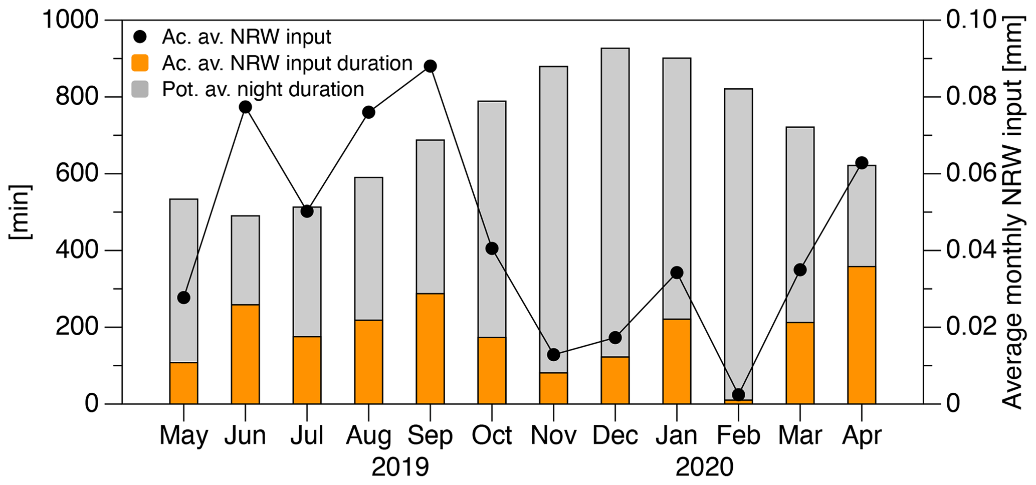
Figure G1Average monthly NRW input with average monthly NRW input duration and average night duration (potential NRW input duration).
Data are stored at the ETH Zurich research collection at https://doi.org/10.3929/ethz-b-000488747 (Riedl, 2021).
AR and WE designed the ML system. AR built the ML system and installed it together with YL. AR carried out maintenance, experiments, data collection, and data analysis. JE and WE added Appendix F. NB and WE commented on the results of data analysis. AR wrote and revised the manuscript, with contributions and feedback by YL, NB, and WE.
The contact author has declared that neither they nor their co-authors have any competing interests.
Publisher's note: Copernicus Publications remains neutral with regard to jurisdictional claims in published maps and institutional affiliations.
We are grateful to Paul Linwood for his excellent work with electronics and installation assistance in the field, and we thank Markus Staudinger, Philip Meier, and Thomas Baur for their technical support. We also thank Patrick Flütsch for constructing the ML pots and lids.
This research has been supported by the Swiss National Science Foundation (grant no. 175733).
This paper was edited by Gerrit H. de Rooij and reviewed by two anonymous referees.
Agam, N. and Berliner, P. R.: Diurnal water content changes in the bare soil of a coastal desert, J. Hydrometeorol., 5, 922–933, https://doi.org/10.1175/1525-7541(2004)005<0922:DWCCIT>2.0.CO;2, 2004.
Agam, N. and Berliner, P. R.: Dew formation and water vapor adsorption in semi-arid environments – A review, J. Arid Environ., 65, 572–590, https://doi.org/10.1016/J.JARIDENV.2005.09.004, 2006.
Alaoui, A. and Eugster, W.: Dual-porosity modeling of groundwater recharge: testing a quick calibration using in situ moisture measurements, Areuse River Delta, Switzerland, Hydrogeol. J., 12, 464–475, https://doi.org/10.1007/s10040-003-0288-y, 2004.
Aparecido, L. M. T., Miller, G. R., Cahill, A. T., and Moore, G. W.: Comparison of tree transpiration under wet and dry canopy conditions in a Costa Rican premontane tropical forest, Hydrol. Process., 30, 5000–5011, https://doi.org/10.1002/hyp.10960, 2016.
Ben-Gal, A. and Shani, U.: A highly conductive drainage extension to control the lower boundary condition of lysimeters, Plant Soil, 239, 9–17, https://doi.org/10.1023/A:1014942024573, 2002.
Berry, Z. C., White, J. C., and Smith, W. K.: Foliar uptake, carbon fluxes and water status are affected by the timing of daily fog in saplings from a threatened cloud forest, Tree Physiol., 34, 459–470, https://doi.org/10.1093/treephys/tpu032, 2014.
Beysens, D.: Dew water, River Publishers, Gistrup Denmark, ISBN 9788793609471, 2018.
Boucher, J. F., Munson, A. D., and Bernier, P. Y.: Foliar absorption of dew influences shoot water potential and root growth in Pinus strobus seedlings, Tree Physiol., 15, 819–823, https://doi.org/10.1093/treephys/15.12.819, 1995.
Brown, R., Mills, A. J., and Jack, C.: Non-rainfall moisture inputs in the Knersvlakte: Methodology and preliminary findings, Water SA, 34, 275–278, https://doi.org/10.4314/wsa.v34i2.183649, 2008.
Chen, L., Meissner, R., Zhang, Y., and Xiao, H.: Studies on dew formation and its meteorological factors, J. Food Agric. Environ., 11, 1063–1068, 2005.
Dawson, T. E.: Fog in the California redwood forest: ecosystem inputs and use by plants, Oecologia, 117, 476–485, https://doi.org/10.1007/s004420050683, 1998.
Dawson, T. E. and Goldsmith, G. R.: The value of wet leaves, New Phytol., 219, 1156–1169, https://doi.org/10.1111/nph.15307, 2018.
Eller, C. B., Lima, A. L., and Oliveira, R. S.: Foliar uptake of fog water and transport belowground alleviates drought effects in the cloud forest tree species, Drimys brasiliensis (Winteraceae), New Phytol., 199, 151–162, https://doi.org/10.1111/nph.12248, 2013.
Engle, R. F. and Granger, C. W. J.: Co-Integration and Error Correction: Representation, Estimation, and Testing, Econometria, 55, 251–276, https://doi.org/10.2307/1913236, 1987.
Eugster, W., Burkard, R., Holwerda, F., Scatena, F. N. and Bruijnzeel, L. A. (Sampurno.: Characteristics of fog and fogwater fluxes in a Puerto Rican elfin cloud forest, Agric. For. Meteorol., 139, 288–306, https://doi.org/10.1016/J.AGRFORMET.2006.07.008, 2006.
Evett, S. R., Warrick, A. W., and Matthias, A. D.: Wall Material and Capping Effects on Microlysimeter Temperatures and Evaporation, Soil Sci., 59, 329–336, 1995.
Feigenwinter, C., Franceschi, J., Larsen, J. A., Spirig, R., and Vogt, R.: On the performance of microlysimeters to measure non-rainfall water input in a hyper-arid environment with focus on fog contribution, J. Arid Environ., 182, 1–13, https://doi.org/10.1016/j.jaridenv.2020.104260, 2020.
Freeze, R. A. and Cherry, J. A.: Groundwater, Prentice-Hall, Englewood Cliffs, N.J., https://doi.org/10.1177/030913338100500412, 1979.
Gerlein-Safdi, C., Koohafkan, M. C., Chung, M., Rockwell, F. E., Thompson, S., and Caylor, K. K.: Dew deposition suppresses transpiration and carbon uptake in leaves, Agric. For. Meteorol., 259, 305–316, https://doi.org/10.1016/j.agrformet.2018.05.015, 2018.
Groh, J., Slawitsch, V., Herndl, M., Graf, A., Vereecken, H., and Pütz, T.: Determining dew and hoar frost formation for a low mountain range and alpine grassland site by weighable lysimeter, J. Hydrol., 563, 372–381, https://doi.org/10.1016/J.JHYDROL.2018.06.009, 2018.
Heusinkveld, B. G., Berkowicz, S. M., Jacobs, A. F. G., Holtslag, A. A. M., and Hillen, W. C. A. M.: An automated microlysimeter to study dew formation and evaporation in arid and semiarid regions, J. Hydrometeorol., 7, 825–832, https://doi.org/10.1175/JHM523.1, 2006.
Imer, D., Merbold, L., Eugster, W., and Buchmann, N.: Temporal and spatial variations of soil CO2, CH4 and N2O fluxes at three differently managed grasslands, Biogeosciences, 10, 5931–5945, https://doi.org/10.5194/bg-10-5931-2013, 2013.
Ishibashi, M. and Terashima, I.: Effects of continuous leaf wetness on photosynthesis: adverse aspects of rainfall, Plant. Cell Environ., 18, 431–438, https://doi.org/10.1111/j.1365-3040.1995.tb00377.x, 1995.
Jacobs, A. F. G., Heusinkveld, B. G., and Berkowicz, S. M.: Dew deposition and drying in a desert system: A simple simulation model, J. Arid Environ., 42, 211–222, https://doi.org/10.1006/jare.1999.0523, 1999.
Jacobs, A. F. G., Heusinkveld, B. G., Wichink Kruit, R. J., and Berkowicz, S. M.: Contribution of dew to the water budget of a grassland area in the Netherlands, Water Resour. Res., 42, W03415, https://doi.org/10.1029/2005WR004055, 2006.
Jia, R. L., Li, X. R., Liu, L. C., Pan, Y. X., Gao, Y. H., and Wei, Y. P.: Effects of sand burial on dew deposition on moss soil crust in a revegetated area of the Tennger Desert, Northern China, J. Hydrol., 519, 2341–2349, https://doi.org/10.1016/j.jhydrol.2014.10.031, 2014.
Jones, H. G.: Monitoring plant and soil water status: established and novel methods revisited and their relevance to studies of drought tolerance, J. Exp. Bot., 58, 119–130, https://doi.org/10.1093/jxb/erl118, 2006.
Kaseke, K. F., Mills, A. J., Brown, R., Esler, K. J., Henschel, J. R., and Seely, M. K.: A Method for Direct Assessment of the “Non Rainfall” Atmospheric Water Cycle: Input and Evaporation From the Soil, Pure Appl. Geophys., 169, 847–857, https://doi.org/10.1007/s00024-011-0328-9, 2012.
Kerr, J. P. and Beardsell, M. F.: Effect of Dew on Leaf Water Potentials and Crop Resistances in a Paspalum Pasture, Agron. J., 67, 596–599, https://doi.org/10.2134/agronj1975.00021962006700050002x, 1975.
Kidron, G. J. and Kronenfeld, R.: Assessing the effect of micro-lysimeters on NRWI: Do micro-lysimeters adequately represent the water input of natural soil?, J. Hydrol., 548, 382–390, https://doi.org/10.1016/j.jhydrol.2017.03.005, 2017.
Kidron, G. J. and Starinsky, A.: Measurements and ecological implications of non-rainfall water in desert ecosystems – A review, Ecohydrology, 12, 1–35, https://doi.org/10.1002/eco.2121, 2019.
Kidron, G. J., Kronenfeld, R., and Starinsky, A.: Wind as a cooling agent: substrate temperatures are responsible for variable lithobiont-induced weathering patterns on west- and east-facing limestone bedrock of the Negev, Earth Surf. Process. Landf., 41, 2078–2084, https://doi.org/10.1002/esp.3973, 2016.
Limm, E., Simonin, K., Bothman, A., and Dawson, T.: Foliar water uptake: a common water acquisition strategy for plants of the redwood forest, Oecologia, 161, 449–459, https://doi.org/10.1007/s00442-009-1400-3, 2009.
Maphangwa, K. W., Musil, C. F., Raitt, L., and Zedda, L.: Differential interception and evaporation of fog, dew and water vapour and elemental accumulation by lichens explain their relative abundance in a coastal desert, J. Arid Environ., 82, 71–80, https://doi.org/10.1016/j.jaridenv.2012.02.003, 2012.
Matimati, I., Musil, C. F., Raitt, L., and February, E.: Non rainfall moisture interception by dwarf succulents and their relative abundance in an inland arid South African ecosystem, Ecohydrology, 6, 818–825, https://doi.org/10.1002/eco.1304, 2013.
McHugh, T. A., Morrissey, E. M., Reed, S. C., Hungate, B. A., and Schwartz, E.: Water from air: An overlooked source of moisture in arid and semiarid regions, Sci. Rep.-UK, 5, 1–6, https://doi.org/10.1038/srep13767, 2015.
Meissner, R., Seeger, J., Rupp, H., Seyfarth, M., and Borg, H.: Measurement of dew, fog, and rime with a high-precision gravitation lysimeter, J. Plant Nutr. Soil Sci., 170, 335–344, https://doi.org/10.1002/jpln.200625002, 2007.
Meissner, R., Rupp, H., and Seyfarth, M.: Advanced technologies in lysimetry, Environ. Sci. Eng., 202979, 159–173, https://doi.org/10.1007/978-3-319-01017-5_8, 2014.
MeteoSchweiz: Klimabulletin Jahr 2019, available at: https://www.meteoschweiz.admin.ch/content/dam/meteoswiss/de/service-und-publikationen/Publikationen/doc/2019_ANN_d.pdf, last access: 1 May 2020.
Meter Group AG: Atmos 41, available at: http://library.metergroup.com/Manuals/20635_ATMOS41_Manual_Web.pdf (last access: 2 April 2021), 2020.
Met Office: National Meteorological Library and Archive Fact Sheet 3 – Water in the atmosphere, available at: https://www.metoffice.gov.uk/binaries/content/assets/metofficegovuk/pdf/research/library-and-archive/library/publications/factsheets/factsheet_3-water-in-the-atmosphere.pdf (last access: 2 April 2021), 2012.
Minnis, P.: Asymmetry in the diurnal variation of surface albedo, IEEE T. Geosci. Remote, 35, 879–891, https://doi.org/10.1109/36.602530, 1997.
Monteith, J. L.: Dew, Q. J. Roy. Meteor. Soc., 83, 322–341, https://doi.org/10.1002/qj.49708335706, 1957.
Munné-Bosch, S. and Alegre, L.: Role of Dew on the Recovery of Water-Stressed Melissa officinalis L. Plants, J. Plant Physiol., 154, 759–766, https://doi.org/10.1016/S0176-1617(99)80255-7, 1999.
Ninari, N. and Berliner, P. R.: The role of dew in the water and heat balance of bare loess soil in the Negev Desert: Quantifying the actual dew deposition on the soil surface, Atmos. Res., 64, 323–334, https://doi.org/10.1016/S0169-8095(02)00102-3, 2002.
Nolz, R., Kammerer, G., and Cepuder, P.: Interpretation of lysimeter weighing data affected by wind, J. Plant Nutr. Soil Sci., 176, 200–208, https://doi.org/10.1002/jpln.201200342, 2013.
Pastorello, G., Trotta, C., Canfora, E., Chu, H., Christianson, D., Cheah, Y. W., Poindexter, C., Chen, J., Elbashandy, A., Humphrey, M., Isaac, P., Polidori, D., Ribeca, A., van Ingen, C., Zhang, L., Amiro, B., Ammann, C., Arain, M. A., Ardö, J., Arkebauer, T., Arndt, S. K., Arriga, N., Aubinet, M., Aurela, M., Baldocchi, D., Barr, A., Beamesderfer, E., Marchesini, L. B., Bergeron, O., Beringer, J., Bernhofer, C., Berveiller, D., Billesbach, D., Black, T. A., Blanken, P. D., Bohrer, G., Boike, J., Bolstad, P. V., Bonal, D., Bonnefond, J. M., Bowling, D. R., Bracho, R., Brodeur, J., Brümmer, C., Buchmann, N., Burban, B., Burns, S. P., Buysse, P., Cale, P., Cavagna, M., Cellier, P., Chen, S., Chini, I., Christensen, T. R., Cleverly, J., Collalti, A., Consalvo, C., Cook, B. D., Cook, D., Coursolle, C., Cremonese, E., Curtis, P. S., D’Andrea, E., da Rocha, H., Dai, X., Davis, K. J., De Cinti, B., de Grandcourt, A., De Ligne, A., De Oliveira, R. C., Delpierre, N., Desai, A. R., Di Bella, C. M., di Tommasi, P., Dolman, H., Domingo, F., Dong, G., Dore, S., Duce, P., Dufrêne, E., Dunn, A., Dušek, J., Eamus, D., Eichelmann, U., ElKhidir, H. A. M., Eugster, W., Ewenz, C. M., Ewers, B., Famulari, D., Fares, S., Feigenwinter, I., Feitz, A., Fensholt, R., Filippa, G., Fischer, M., Frank, J., Galvagno, M., Gharun, M., Gianelle, D., Gielen, B., Gioli, B., Gitelson, A., Goded, I., Goeckede, M., Goldstein, A. H., Gough, C. M., Goulden, M. L., Graf, A., Griebel, A., Gruening, C., Grünwald, T., Hammerle, A., Han, S., Han, X., Hansen, B. U., Hanson, C., Hatakka, J., He, Y., Hehn, M., Heinesch, B., Hinko-Najera, N., Hörtnagl, L., Hutley, L., Ibrom, A., Ikawa, H., Jackowicz-Korczynski, M., Janouš, D., Jans, W., Jassal, R., Jiang, S., Kato, T., Khomik, M., Klatt, J., Knohl, A., Knox, S., Kobayashi, H., Koerber, G., Kolle, O., Kosugi, Y., Kotani, A., Kowalski, A., Kruijt, B., Kurbatova, J., Kutsch, W. L., Kwon, H., Launiainen, S., Laurila, T., Law, B., Leuning, R., Li, Yingnian, Liddell, M., Limousin, J. M., Lion, M., Liska, A. J., Lohila, A., López-Ballesteros, A., López-Blanco, E., Loubet, B., Loustau, D., Lucas-Moffat, A., Lüers, J., Ma, S., Macfarlane, C., Magliulo, V., Maier, R., Mammarella, I., Manca, G., Marcolla, B., Margolis, H. A., Marras, S., Massman, W., Mastepanov, M., Matamala, R., Matthes, J. H., Mazzenga, F., McCaughey, H., McHugh, I., McMillan, A. M. S., Merbold, L., Meyer, W., Meyers, T., Miller, S. D., Minerbi, S., Moderow, U., Monson, R. K., Montagnani, L., Moore, C. E., Moors, E., Moreaux, V., Moureaux, C., Munger, J. W., Nakai, T., Neirynck, J., Nesic, Z., Nicolini, G., Noormets, A., Northwood, M., Nosetto, M., Nouvellon, Y., Novick, K., Oechel, W., Olesen, J. E., Ourcival, J. M., Papuga, S. A., Parmentier, F. J., Paul-Limoges, E., Pavelka, M., Peichl, M., Pendall, E., Phillips, R. P., Pilegaard, K., Pirk, N., Posse, G., Powell, T., Prasse, H., Prober, S. M., Rambal, S., Rannik, Ü., Raz-Yaseef, N., Reed, D., de Dios, V. R., Restrepo-Coupe, N., Reverter, B. R., Roland, M., Sabbatini, S., Sachs, T., Saleska, S. R., Sánchez-Cañete, E. P., Sanchez-Mejia, Z. M., Schmid, H. P., Schmidt, M., Schneider, K., Schrader, F., Schroder, I., Scott, R. L., Sedlák, P., Serrano-Ortíz, P., Shao, C., Shi, P., Shironya, I., Siebicke, L., Šigut, L., Silberstein, R., Sirca, C., Spano, D., Steinbrecher, R., Stevens, R. M., Sturtevant, C., Suyker, A., Tagesson, T., Takanashi, S., Tang, Y., Tapper, N., Thom, J., Tiedemann, F., Tomassucci, M., Tuovinen, J.P., Urbanski, S., Valentini, R., van der Molen, M., van Gorsel, E., van Huissteden, K., Varlagin, A., Verfaillie, J., Vesala, T., Vincke, C., Vitale, D., Vygodskaya, N., Walker, J. P., Walter-Shea, E., Wang, H., Weber, R., Westermann, S., Wille, C., Wofsy, S., Wohlfahrt, G., Wolf, S., Woodgate, W., Li, Yuelin, Zampedri, R., Zhang, J., Zhou, G., Zona, D., Agarwal, D., Biraud, S., Torn, M., and Papale, D.: The FLUXNET2015 dataset and the ONEFlux processing pipeline for eddy covariance data, Sci. Data, 7, 225, https://doi.org/10.1038/s41597-020-0534-3, 2020.
Pedregosa, F., Varoquaux, G., Gramfort, A., Michel, V., Thirion, B., and Grisel, O.: Scikit-learn: Machine learning in Python, J. Mach. Learn. Res., 12, 2825–2830, 2011.
Rawls, W, J., Gish, T. J., and Brakensiek, D. L.: Estimating soil water retention from soil physical properties and characteristic, in: Advances in Soil Science, edited by: Stewart, B. A., Springer, New York, 213–234, https://doi.org/10.1007/978-1-4612-3144-8_5, 1991.
Richards, K.: Observation and simulation of dew in rural and urban environments, Prog. Phys. Geogr., 28, 76–94, https://doi.org/10.1191/0309133304pp402ra, 2004.
Riedl, A.: Data from: High accuracy weighing micro-lysimeter system for long-term measurements of non-rainfall water inputs to grasslands, ETH Zürich [data set], https://doi.org/10.3929/ethz-b-000488747, 2021.
Ritter, A., Regalado, C. M., and Aschan, G.: Fog reduces transpiration in tree species of the Canarian relict heath-laurel cloud forest (Garajonay National Park, Spain), Tree Physiol., 29, 517–528, https://doi.org/10.1093/treephys/tpn043, 2009.
Sautier, S. C.: Zusammensetzung und Produktivität der Vegetation im Gebiet der ETHZ-Forschungsstation Früebüel (ZG), MSc Thesis, Inst. Geogr. Univ. Zurich, 2007.
Seabold, S. and Perktold, J.: Statsmodels: Econometric and Statistical Modeling with Python, Proceedings of the 9th Python in Science Conference, https://doi.org/10.25080/majora-92bf1922-011, 2010.
Slatyer, R. O.: The absorption of water by plants, Nature, 30, 7–9, https://doi.org/10.1038/030007b0, 1960.
Stiehl-Braun, P. A., Hartmann, A. A., Kandeler, E., Buchmann, N., and Niklaus, P. A.: Interactive effects of drought and N fertilization on the spatial distribution of methane assimilation in grassland soils, Glob. Chang. Biol., 17, 2629–2639, https://doi.org/10.1111/j.1365-2486.2011.02410.x, 2011.
Thornthwaite, C. W.: An Approach toward a Rational Classification of Climate, Geogr. Rev., 38, 55–94, https://doi.org/10.1097/00010694-194807000-00007, 1948.
Timlin, D. J., Williams, R. D., Ahuja, L. R., and Heathman, G. C.: Simple parametric methods to estimate soil water retention and hydraulic conductivity, in: Development of pedotransfer functions in soil hydrology, edited by: Pachepsky, Y., Elsevier, Amsterdam, New York, 71–93, https://doi.org/10.1016/s0166-2481(04)30005-x, 2004.
Uclés, O., Villagarcía, L., Cantón, Y., and Domingo, F.: Microlysimeter station for long term non-rainfall water input and evaporation studies, Agric. For. Meteorol., 182–183, 13–20, https://doi.org/10.1016/j.agrformet.2013.07.017, 2013.
Vesala, T., Sevanto, S., Grönholm, T., Salmon, Y., Nikinmaa, E., Hari, P., and Hölttä, T.: Effect of Leaf Water Potential on Internal Humidity and CO2 Dissolution: Reverse Transpiration and Improved Water Use Efficiency under Negative Pressure, Front. Plant Sci., 8, 54, https://doi.org/10.3389/fpls.2017.00054, 2017.
Waggoner, P. E., Begg, J. E., and Turner, N. C.: Evaporation of dew, Agric. Meteorol., 6, 227–230, https://doi.org/10.1016/0002-1571(69)90007-7, 1969.
Wang, L., Kaseke, K. F., Ravi, S., Jiao, W., Mushi, R., Shuuya, T., and Maggs-Kölling, G.: Convergent vegetation fog and dew water use in the Namib Desert, Ecohydrology, 12, 1–11, https://doi.org/10.1002/eco.2130, 2019.
Westerhuis, S., Fuhrer, O., Cermak, J., and Eugster, W.: Identifying the key challenges for fog and low stratus forecasting in complex terrain, Q. J. Roy. Meteor. Soc., 146, 3347–3367, https://doi.org/10.1002/qj.3849, 2020.
Yates, D. J. and Hutley, L. B.: Foliar uptake of water by wet leaves of Sloanea woollsii, an Australian subtropical rainforest tree, Aust. J. Bot., 43, 157–167, https://doi.org/10.1071/BT9950157, 1995.
Zeeman, M. J., Hiller, R., Gilgen, A. K., Michna, P., Plüss, P., Buchmann, N., and Eugster, W.: Management and climate impacts on net CO2 fluxes and carbon budgets of three grasslands along an elevational gradient in Switzerland, Agric. For. Meteorol., 150, 519–530, https://doi.org/10.1016/j.agrformet.2010.01.011, 2010.
Zhan, T. L. T., Qiu, Q. W., and Xu, W. J.: Analytical solution for infiltration and deep percolation of rainwater into a monolithic cover subjected to different patterns of rainfall, Comput. Geotech., 77, 1–10, https://doi.org/10.1016/j.compgeo.2016.03.008, 2016.
Zhang, J., Zhang, Y.-M., Downing, A., Cheng, J.-H., Zhou, X.-B., and Zhang, B.-C.: The influence of biological soil crusts on dew deposition in Gurbantunggut Desert, Northwestern China, J. Hydrol., 379, 220–228, https://doi.org/10.1016/j.jhydrol.2009.09.053, 2009.
Zhang, Q., Wang, S., Yang, F. L., Yue, P., Yao, T., and Wang, W. Y.: Characteristics of Dew Formation and Distribution, and Its Contribution to the Surface Water Budget in a Semi-arid Region in China, Boundary-Layer Meteorol., 154, 317–331, https://doi.org/10.1007/s10546-014-9971-x, 2014.
Zhang, Q., Wang, S., Yue, P., and Wang, R.: A measurement, quantitative identification and estimation method(QINRW) of non-rainfall water component by lysimeter, MethodsX, 6, 2873–2881, https://doi.org/10.1016/j.mex.2019.11.012, 2019.
- Abstract
- Introduction
- Material and methods
- Results
- Discussion
- Summary and conclusions
- Appendix A: Location map
- Appendix B: Installation procedure and soil monolith preparation
- Appendix C: Data collection, storage, and delivery
- Appendix D: Load cell data low-pass filtering
- Appendix E: Drainage-water flow of ML pots
- Appendix F: Duration of drainage-water flow after heavy rainfall (saturated soils)
- Appendix G: NRW inputs vs. night-time duration
- Data availability
- Author contributions
- Competing interests
- Disclaimer
- Acknowledgements
- Financial support
- Review statement
- References