the Creative Commons Attribution 4.0 License.
the Creative Commons Attribution 4.0 License.
 | 30 Nov 2022
Linking the complementary evaporation relationship with the Budyko framework for ungauged areas in Australia
Daeha Kim
Minha Choi
While the calibration-free complementary relationship (CR) has performed excellently in predicting terrestrial evapotranspiration (ETa), how to determine the Priestley–Taylor coefficient (αe) is a remaining question. In this work, we evaluated this highly utilizable method, which only requires atmospheric data, with in situ flux observations and basin-scale water-balance estimates (ETwb) in Australia, proposing how to constrain it with a traditional Budyko equation for ungauged locations. We found that the CR method with a constant αe transferred from fractional wet areas performed poorly in reproducing the mean annual ETwb in unregulated river basins, and it underperformed advanced physical, machine-learning, and land surface models in closing grid-scale water balance. This problem was remedied by linking the CR method with a traditional Budyko equation that allowed for an upscaling of the optimal αe from gauged basins to ungauged locations. The combined CR–Budyko framework enabled us to reflect climate conditions in αe, leading to more plausible ETa estimates in ungauged areas. The spatially varying αe conditioned by local climates enabled the CR method to outperform the three ETa models in reproducing the grid-scale ETwb across the Australian continent. We argued here that the polynomial CR with a constant αe could result in biased ETa, and it can be constrained by a traditional Budyko equation for improvement.
- Article
(6412 KB) - Full-text XML
- BibTeX
- EndNote


Evapotranspiration (ETa) plays a pivotal role in water and energy exchanges between the land and the atmosphere. On the global scale, more than 60 % of terrestrial precipitation (P) returns to the atmosphere through plants' vascular systems and soil pores while consuming over 70 % of surface net radiation (Trenberth et al., 2007, 2009). Since it is tightly coupled with carbon cycles, abnormally low ETa would indicate food insecurity and low ecosystem sustainability (Jasechko, 2018; Kyatengerwa et al., 2020; Pareek et al., 2020; Swann et al., 2016). In severe cases, ETa limited by deficient soil moisture can lead to extreme heatwaves that further propagate the water deficit in space and time (Miralles et al., 2014; Mueller and Seneviratne, 2012; Schumacher et al., 2022).
Despite great community efforts for sharing in situ observations (e.g., Baldocchi, 2020; Novick et al., 2018), ETa gauging networks are unevenly established over land surfaces and often subjected to error sources (e.g., unclosed energy balance) and limited data lengths (Ma et al., 2021). Inevitably, modeling approaches are needed to predict ETa in ungauged or poorly gauged areas or to characterize it on a long timescale in a large area. Hence, various approaches have been proposed, including physical models (e.g., Martens et al., 2017; Zhang et al., 2016), machine-learning techniques (e.g., Jung et al., 2019; Tramontana et al., 2016), and conceptual land surface schemes (e.g., Guimberteau et al., 2018; Haverd et al., 2018).
Those modeling approaches typically require P data and land surface information (e.g., remote-sensing vegetation indices) to quantify available soil moisture to the vaporization process. However, due in part to uncertainty associated with P data (Sun et al., 2018) and model structures (Samaniego et al., 2017; Zhang et al., 2019), resulting ETa estimates have shown substantial disparities. In the comprehensive intercomparison by Pan et al. (2020), for example, the 14 advanced land surface models generated the global mean ETa varying widely between 450 and 700 mm a−1. Such a large incongruity in modeled ETa was also found by the earlier Global Soil Wetness Project (Schlosser and Gao, 2010), suggesting that an alternative method is necessary to circumvent the uncertainty sources.
A practical method to simulate ETa without P data and land surface schemes is the complementary relationship (CR) of evaporation (Bouchet, 1963). It uses the evident fact that the air over a water-limited surface amplifies its vapor pressure deficit (VPD), while this effect disappears when the same surface is amply wet (Chen and Buchberger, 2018; Ramírez et al., 2005; Zhou et al., 2019). Based on the atmospheric self-adjustment, numerous equations have been formulated to predict ETa only using routine meteorological data (e.g., Anayah and Kaluarachchi, 2014; Crago and Crowley, 2005; Crago and Qualls, 2013; Hobbins et al., 2004; Huntington et al., 2011; Kahler and Brutsaert, 2006 among others). In particular, the definitive derivation by Brutsaert (2015) and the following modifications (Crago et al., 2016; Crago and Qualls, 2021; Szilagyi, 2021; Szilagyi et al., 2017) provided strong physical foundations to the early principle of Bouchet (1963). They have excellently predicted ETa at various spatial and temporal scales (e.g., Brutsaert et al., 2017, 2020; Crago and Qualls, 2018; Ma et al., 2019, 2021; Ma and Szilagyi, 2019) and allowed users to assess vegetation droughts over national and continental areas (e.g., Kim et al., 2019, 2021; Kyatengerwa et al., 2020).
Nevertheless, definitive CRs still require at least some ETa data to calibrate the parameters that determine the hypothetical wet-surface evaporation (ETw; Qualls and Crago, 2020); thus, they are not fully free of P data or parameterization. For instance, Brutsaert et al. (2020) calibrated the single parameter of the CR of Brutsaert (2015) with flux observations and basin-scale P and runoff (Q) data to estimate mean annual ETa across the globe. For evaluating four definitive CRs from the derivation of Brutseart (2015), Crago et al. (2022) also calibrated their parameters against eddy-covariance flux observations. To date, Szilagyi et al. (2017) have proposed the only CR formulation that purely uses routine meteorological data; however, it depends on a questionable assumption that the parameter for ETw is constant over a large continental area, being counterfactual to experimental studies on the Priestley and Taylor (1972) coefficient (e.g., Assouline et al., 2016; Baldocchi et al., 2016; Parlange and Katul, 1992; Wang et al., 2014). Given the complex space–time links between climate, soil, and vegetation (Hagedorn et al., 2019; Mekonnen et al., 2019; Rodriguez-Iturbe, 2000), the aerodynamic component of ETw is unlikely represented by a fixed fraction of the net radiation.
Owing to the data required for parameter calibration, the state-of-the-art CR formulations might not be applicable in ungauged locations. In part, this problem can be mended by an additional constraint for determining the essential parameters, and the traditional Budyko framework can come into play. A Budyko function (e.g., Fu, 1981; Yang et al., 2008) explains the mean ratio of ETa to P (i.e., surface water balance) simply by climatological aridity and a few implicit parameters, simultaneously closing the surface energy budget (Mianabadi et al., 2020). Although Bouchet's principle has often been linked with the water balance described by Budyko functions (e.g., Carmona et al., 2016; Chen and Buchberger, 2018; Lhomme and Moussa, 2016; Zhang and Brutsaert, 2021), this theoretical link has been ignored when predicting ETa by the definitive CRs. Kim and Chun (2021) explicitly showed that the atmospheric self-adjustment is tightly coupled with the climatological aridity within a Budyko function. This implies that the optimal parameter for a definitive CR should vary with climates rather than staying constant.
In this work, we showed that a Budyko equation could become an important physical constraint when predicting ETa by a definitive CR over a continental area. Here, a practical approach was proposed to determine the parameter reasonably in ungauged locations via a case study for the Australian continent, where the performance of the CR method remained unknown in many parts. Based on the analytical relationship between the CR and the Budyko framework, we showed why the parameter of the CR is not independent of local climate conditions and addressed how to reflect spatially varying climates in its essential parameter.
2.1 The polynomial CR by Szilagyi et al. (2017)
For the case study, we employed the calibration-free CR formulated by Szilagyi et al. (2017). It describes the atmospheric self-adjustment to surface moisture conditions using three evaporation rates, namely, ETa, ETw, and the potential evaporation (ETp). ETa is the actual moisture flux from a land surface to the atmosphere, and ETw is the hypothetical ETa rate that should occur with ample water availability. ETp is the atmospheric capacity to receive water vapor that responds actively to soil moisture conditions. By defining the two dimensionless variables as and , Szilagyi et al. (2017) derived a polynomial function from four definitive boundary conditions.
Under ample water conditions, ETp does not deviate from ETw and ETa (i.e., ETp = ETw = ETa); hence, the corresponding zero-order boundary condition is (i) y=1 for x=1. In contrast, ETa must be nil over a desiccated surface (i.e., y=0), and by energy balance, the surface net radiation should be fully transformed to the sensible heat flux. Then, the atmospheric VPD would be amplified at the maximum level with the same net radiation and wind speed. Defining the maximum ETp rate as Epmax, another zero-order boundary condition is given as (ii) y=0 for . When x=1 (i.e., ample water), changes in ETa would be controlled by changes in ETw, yielding a first-order boundary condition as (iii) for x=1. Over a desiccated surface, ETa stays at zero, even when ETw changes; thus, another first-order boundary condition becomes (iv) for x=xmin. The simplest polynomial equation satisfying the four boundary conditions is
where X rescales the variable x into [0, 1] as
Equation (1) allows users to estimate ETa with no land surface information because ETp, ETw, and Epmax are all obtainable from a set of net radiation, air temperature, dew-point temperature, and wind speed data. ETp and Epmax can be estimated by the Penman (1948) equation:
where Δ(⋅) is the slope of the saturation vapor pressure curve (kPa ∘C−1); Ta is the mean air temperature (∘C); γ is the psychrometric constant (kPa ∘C−1); Rn is the surface net radiation less the soil heat flux (MJ m−2 d−1); λv is the latent heat of vaporization (MJ kg−1); fu=2.6 (1+0.54 u2) is the Rome wind function (mm d−1 kPa−1), where u2 is the 2 m wind speed (m s−1); and VPD is calculated by es (Ta) minus es (Tdew), where es(⋅) is the saturation vapor pressure (kPa), and Tdew is the dew-point temperature (∘C).
Tdry in Eq. (4) is the air temperature (∘C) at which the lower atmosphere is devoid of humidity presumably by the adiabatic drying process:
where Twb is the wet-bulb temperature (∘C) at which the saturation vapor pressure curve intersects with the adiabatic wetting line. Thus, it is obtained by
To estimate ETw in Eq. (2), the Priestley–Taylor (1972) equation has been a typical choice (e.g., Brutsaert, 2015; Crago et al., 2016; Han and Tian, 2018; Szilagyi et al., 2017):
where αe is the Priestley–Taylor coefficient ranging usually within [1.10, 1.32] (Szilagyi et al., 2017), and Tw is the wet-environment air temperature (∘C). Tw can be approximated with the wet-surface temperature (Tws) because the vertical air temperature gradient is negligible under a wet environment. Given its independence on areal extent (Szilagyi and Schepers, 2014), Tws can be approximated by the implicit Bowen ratio (β) of a small wet patch:
Equation (8) assumes that the available radiation for the wet patch is close to that of the drying surface (Szilagyi et al., 2017). Tws might be higher than Ta when the air is close to saturation. In such a case, Tws should be capped by Ta when calculating ETw.
The single parameter of the polynomial CR, i.e., αe, is analytically obtainable by inserting the Priestley–Taylor equation into the Bowen ratio of a wet environment (Szilagyi et al., 2017) as
where αe must fall within the theoretical limit of [1, (Priestley and Taylor, 1972).
2.2 The analytical relationship between the polynomial CR and a Budyko function
Since Eq. (9) is only applicable in a wet environment, Szilagyi et al. (2017) identified wet locations in a continental area based on the fact that the air close to saturation should have high relative humidity (RH) with Tws>Ta. Thus, they calculated αe values at locations with RH > 90 % and ∘C, and the average value was used to predict ETa for a continental area. However, the spatially constant αe is unlikely suitable in such a large area under diverse climates because the equilibrium between the atmosphere and the underlying surface is intertwined with the partitioning of P to ETa and Q over the surface.
Kim and Chun (2021) analytically related Eq. (1) with the traditional Turc–Mezentsev equation and found that the self-adjustment of ETp (i.e., x) is tightly linked with climatological aridity and land properties. For the independence between P and “the possible maximum ETa” of the Budyko framework, Kim and Chun (2021) reformulated the traditional equation with instead of the commonly used aridity index () as
where the parameter n implicitly represents the factors affecting the P partitioning other than the climatic drivers. When dividing Eq. (10) by Φ, it is found that the Budyko Eq. (10) is intertwined with the Eq. (1) of the CR:
Equation (11) implies that the self-adjustment of ETp (i.e., x) is tightly related with the climatic condition (i.e., Φ) and the implicit land property (i.e., n).
While the x and n can be achievable from a set of ETa, ETp, Epmax, and P values by inverting Eq. (11), such an approach is not applicable in locations with no ETa data. To quantify x values only using ETp, Epmax, and P, Kim and Chun (2021) developed a regression equation between x and Φ, xmin, and n values from 513 gauged river basins around the world. We used the same regression-based regionalization. Considering , the nonlinear expression in Eq. (11) can be approximated by a multiple regression as
where is the approximate ratio of ETw to ETp, and b0, b1, and b2 are the intercept and the regression coefficients. Since the implicit parameter n is unavailable in ungauged locations, Eq. (12) needs to be further simplified by neglecting the last term:
where c0, c1, and c2 are the intercept and the coefficients of the approximated regression.
If is known by the regression by Eq. (13), the parameter αe can be estimated using the Priestley–Taylor equation as
where is the Priestley–Taylor coefficient that approximately satisfies the CR and the Budyko equations together, and ETeq is the equilibrium ETa (mm d−1) at which VPD is nil under a wet environment. It should be noted that P, ETp, Epmax, and ETeq within Eqs. (10)–(13) must be on a timescale where the Turc–Mezentsev equation is valid (typically longer than a year), and is still bounded within [1, .
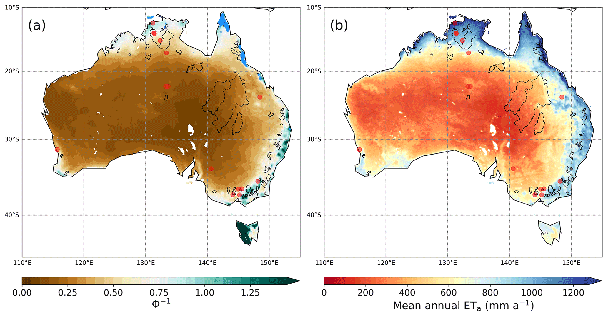
Figure 1Spatial distributions of (a) the reciprocals of aridity index and (b) the mean annual ETa for 1998–2014 predicted by the CR with αe=1.15. The red circles and the gray polygons are the locations of 15 flux towers and the boundaries of 71 CAMELS basins. The blue-colored points in (a) indicate the wet cells with RH > 90 % and ∘C. CR ETa was calculated at the grid cells where the land fraction was larger than 50 %.
2.3 Atmospheric forcing, eddy-covariance, and runoff data
We examined the CR–Budyko combined framework in the Australian continent lying within (10–45∘ S, 113–155∘ E). The required atmospheric forcing data (Rn, Ta, Tdew, and u2) were collected from the advanced ERA5-Land reanalysis archive (Muñoz-Sabater et al., 2021) of the European Centre for Medium-Range Weather Forecasts (https://cds.climate.copernicus.eu; last access: 10 December 2021). The monthly averages of surface latent and sensible heat fluxes, 2 m air temperature, 2 m dew-point temperature, and 10 m U and V wind speed components at were downloaded for 1981–2020. Rn was calculated by summing the two heat fluxes, and the 10 m wind speed components were converted to u2 using the logarithmic wind profile (Allen et al., 1998).
We also collected the Australian edition of the Catchment Attributes and Meteorology for Large sample Studies (CAMELS; Fowler et al., 2021) series of datasets (https://doi.org/10.1594/PANGAEA.921850). The CAMELS datasets comprise daily time series of 19 hydrometeorological variables at 222 unregulated river basins in Australia up to 2014, and we selected the 71 basins larger than 500 km2 to contain at least five CR ETa estimates within the boundaries. The water-balance ETa (ETwb) (i.e., ET of each basin was calculated for the two periods of 1981–1997 and 1998–2014. The mean annual ETwb for the former period was used for the regressions with Eqs. (12) and (13), and the predicted ETa was evaluated against the latter.
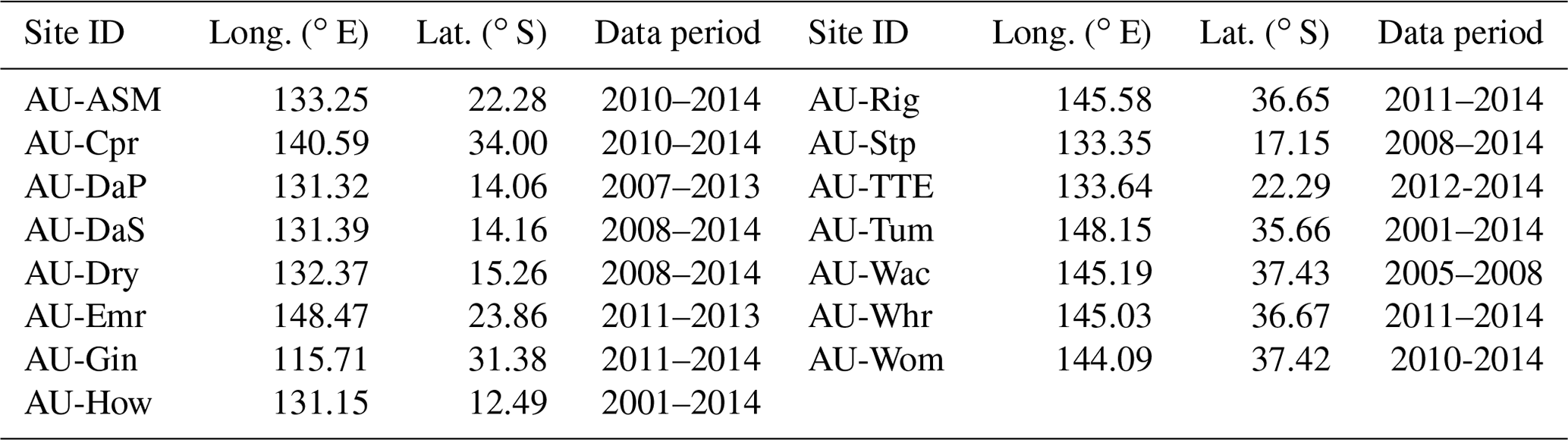
As a point-scale evaluation dataset, the annual flux observations were taken from the 15 eddy-covariance stations (Table 1) included in the FLUXNET2015 archive (https://fluxnet.org/; last access: 1 July 2021). We chose the flux towers with two or more annual means and adopted the energy-balance-corrected latent heat flux observations with the quality measures “LE_F_MDSQC” higher than 0.70. Given the fine resolution of the ERA5-Land forcing data, we believed that the ETa estimates by CR could be directly compared with the point-scale observations.
In addition, as a grid-scale evaluation reference, the SILO P data at were collected from the Queensland government (https://www.longpaddock.qld.gov.au/silo/gridded-data; last access: 1 June 2021) together with the Global RUNoff (GRUN) ENSEMBLE (Ghiggi et al., 2021) (https://doi.org/10.6084/m9.figshare.12794075; last access: 1 October 2021). The global Q data were produced at using a machine-learning algorithm trained by in situ streamflow observations, and potential biases were reduced by simulations with 21 sets of atmospheric forcing (Ghiggi et al., 2021). The SILO P was used to calculate Φ at each grid of the forcing data. After bilinearly unifying the resolutions of SILO P and GRUN Q data, we also calculated the mean annual ETwb for 1998–2014 at over the entire Australian continent.
Against the grid-scale ETwb estimates, performance of the polynomial CR was also compared with three ETa products from a physical, a machine-learning, and a land surface model. The physical model was the Global Land Evaporation Amsterdam Model (GLEAM) v3.2 (Martens et al., 2017; https://www.gleam.eu; last access: 3 June 2020) based on the Priestley–Taylor equation constrained by microwave-derived soil moisture, surface temperature, and vegetation optical depth. The machine-learning ETa product was the FluxCom (http://www.fluxcom.org/; last access: 18 March 2019) that upscaled in situ observations at 224 eddy-covariance towers using 11 algorithms (Jung et al., 2019). We used the version forced by the CRUNCEPv8 that has the longest data length from 1950 to 2016. The land surface model product was the ERA5-Land monthly ETa (https://cds.climate.copernicus.eu; last access: 7 July 2021) simulated by the advanced Hydrology Tiled ECMWF Scheme for Surface Exchanges over Land (Balsamo et al., 2015). All the modeled ETa datasets were bilinearly regridded to for 1998–2014 to be compared with the grid-scale ETwb data.
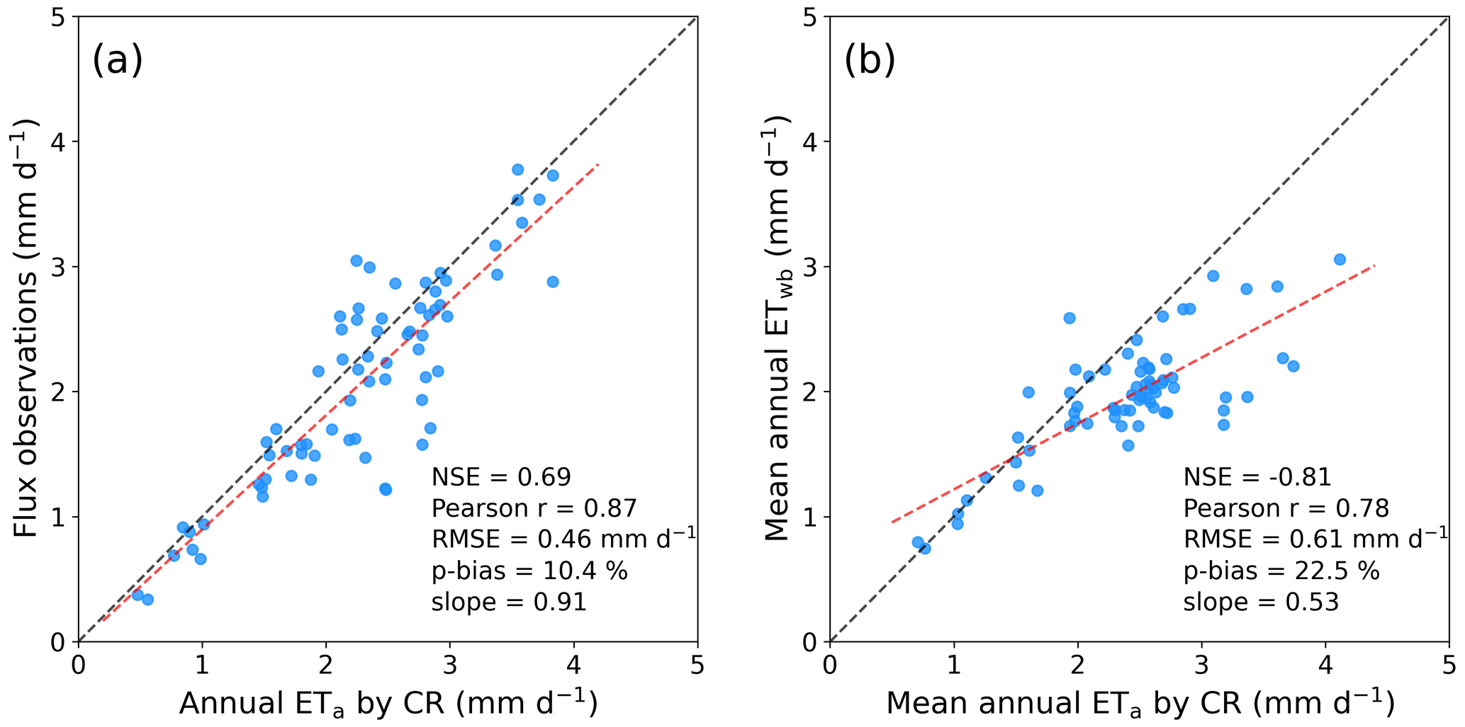
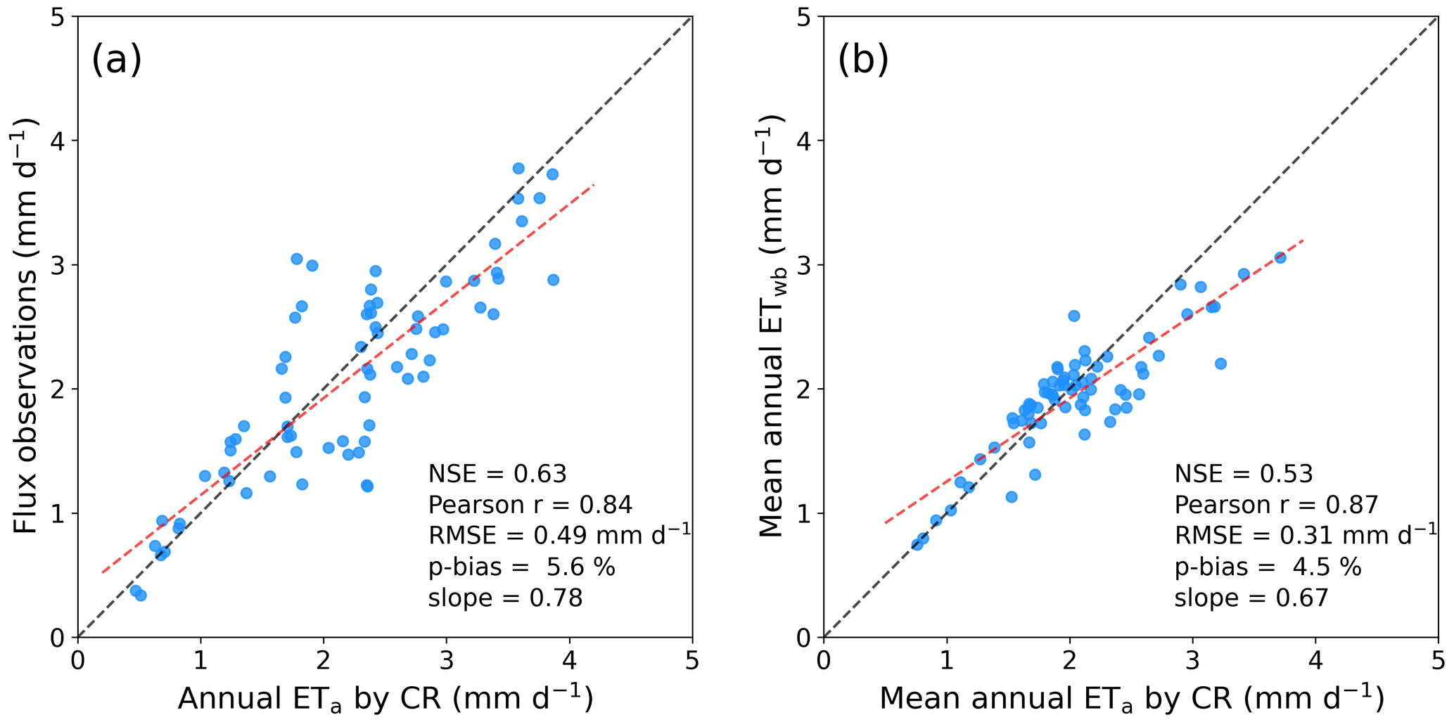
Figure 2The 1:1 comparison between the CR ETa estimates with αe=1.15 and (a) the annual FLUXNET2015 observations and (b) the mean annual ETwb of the 71 CAMELS basins for 1998–2014.
3.1 Performance of the calibration-free CR in Australia
Figure 1a depicts the spatial distribution of the inverted aridity index ( that can traditionally categorize climate conditions. The mean ratios between SILO P and ETp for 1998–2014 indicated that 83 % of the Australian land surfaces were under arid () and semi-arid climates (). Semi-humid () and humid climates () were only found in the northern and southeastern coastal areas and the southwestern edge where major cities and agricultural lands have developed. Despite the high aridity, hyper-arid climates () were not found in Australia.
We first examined the calibration-free approach by Szilagyi et al. (2017) that only uses the meteorological forcing inputs. The blue-colored points in Fig. 1a are the locations with RH > 90 % and Tws > Ta+2 ∘C, at which the αe values from Eq. (9) were within 1.15 ± 0.047 (mean ± standard deviation). Though the two conditions were met in some mountainous areas in the southeastern part, we excluded them because unexpectedly high αe values were obtained. The mean αe=1.15 fell within the theoretical limits and was equal to the value used in the prior studies in China (Ma et al., 2019) and the conterminous United States (Ma and Szilagyi, 2019).
Using the CR with αe=1.15, we predicted ETa over the entire Australian continent (Fig. 1b). The distribution of the resulting mean ETa for 1998–2014 was coherent with that of Φ−1. The mean CR ETa ranged in 262 ± 85.3 and 547 ± 173 mm a−1 under arid and semi-arid climates, respectively. On the other hand, CR ETa in semi-humid and humid locations was much higher, at 886 ± 187 mm a−1 and 1010 ± 213 mm a−1, respectively. The calibration-free CR predicted the continental mean ETa to be as high as 489 mm a−1 for 1981–2012, and it was about 11.3 % higher than the estimate for the same period (439 mm a−1) by Zhang et al. (2016). The mean fraction of ETa to P for 1998–2014 (97 %) was larger than the typical ETa value in Australia (∼90 %; Glenn et al., 2011), implicating that the constant αe=1.15 seemed to make the CR overrate ETa.

Figure 4The scatter plots between the x estimated by CR with ETwb for 1981–1997 and the corresponding (a) Φ, (b) ET, and (c) n values and (d) the 1:1 plot between the x from CR and the predicted by Eq. (17). The red x symbols are the outliers excluded from the regression analysis.
The overestimation of the calibration-free CR was confirmed by the flux observations and the basin-scale ETwb (Fig. 2). The percent bias (p-bias) of CR ETa to the point-scale annual ETa was +10.4 %, while it became more than doubled when compared to the basin-scale ETwb. Though the Pearson correlation coefficients (Pearson r) were significantly high between the CR ETa and the two evaluation references, the low Nash–Sutcliffe efficiency (NSE) to ETwb implies that the CR method could perform poorly in wet river basins. The regression slopes in Fig. 2 also indicate that the calibration-free CR tends to increasingly overestimate as climate becomes wetter. The root mean square error (RMSE) of CR ETa to ETwb was higher than to the point observations. Although it appeared to perform acceptably at the 15 flux towers, the CR method produced considerable biases in the 71 CAMELS basins. The performance measures were not as excellent as the same CR method had shown in the United States (Ma et al., 2021; Ma and Szilagyi, 2019; Kim et al., 2019) and in China (Ma et al., 2019).
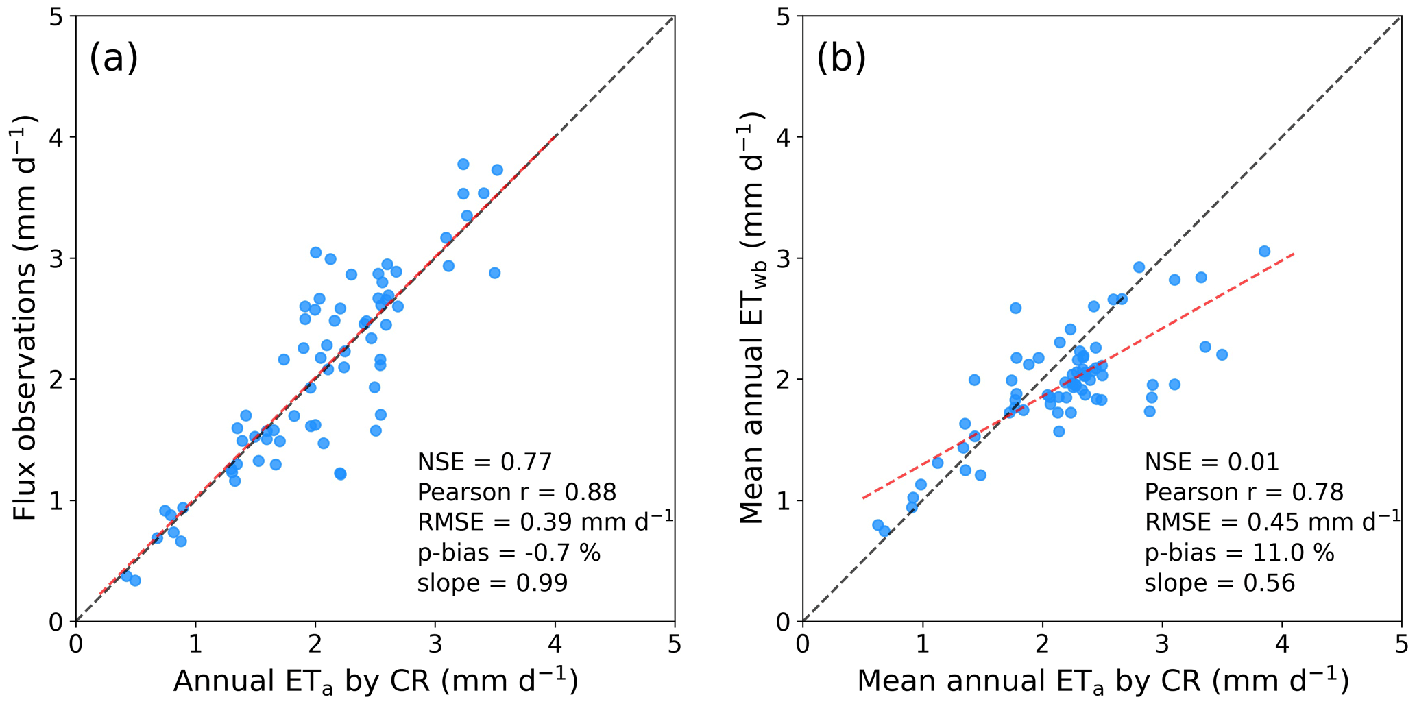
One may argue that the mean αe derived from fractional wet areas is unlikely representative of the large Australian continent, and this might introduce the biases to CR ETa estimates. Hence, we re-simulated CR ETa with the estimate by Ma et al. (2021) (αe=1.10) from a global-scale analysis. Figure 3a shows that the predicted ETa became nearly unbiased at the 15 flux tower locations and seemingly suggests that the decreased αe could become a solution to improving the CR method. Nevertheless, the fixed αe still made the CR overestimate ETa in the CAMELS basins under (semi-)humid climates, albeit slightly ameliorated (Fig. 3b).
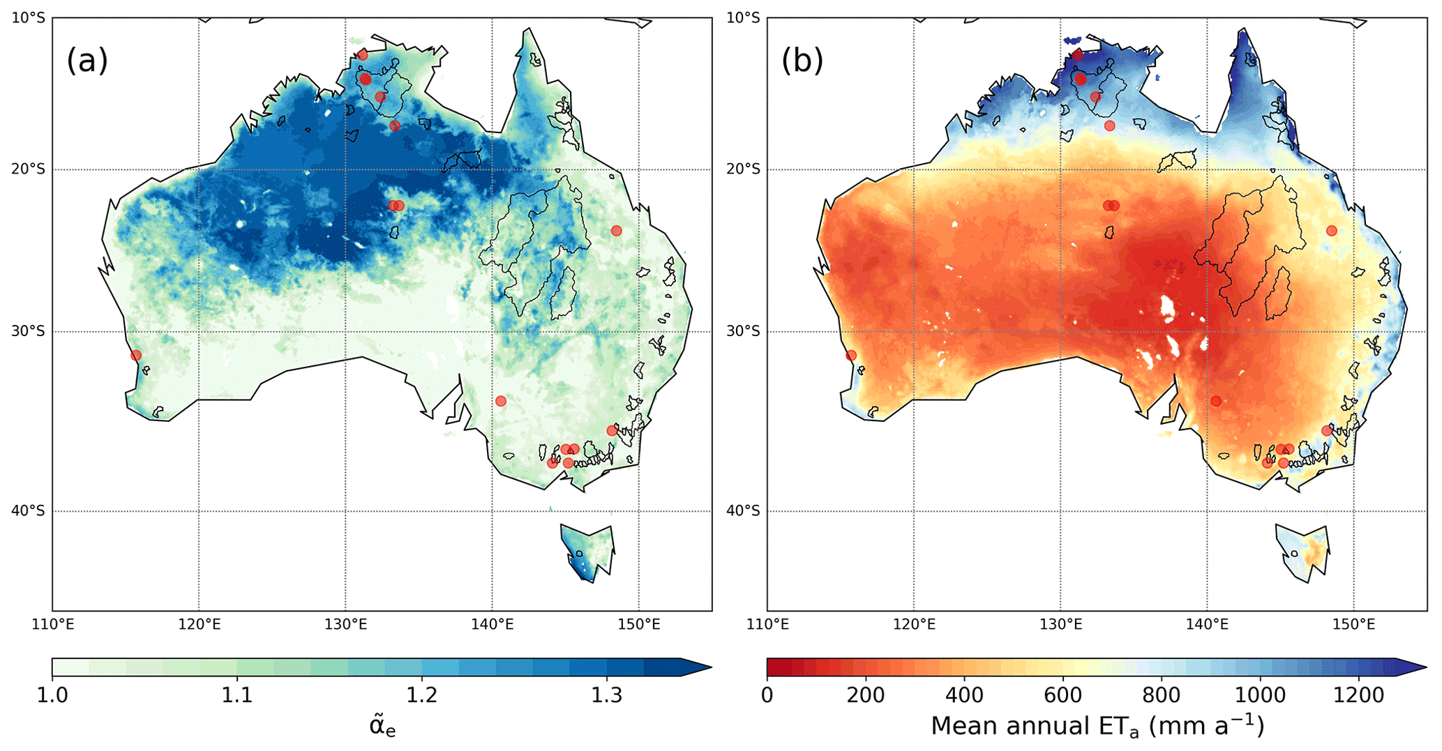
Figure 5Distributions of (a) the values from Eq. (17) and (b) the mean annual ETa for 1998–2014 by the CR method with the values.
3.2 The empirical relationship between and climate conditions
Figures 2 and 3 imply that the calibration-free CR with a fixed αe was unlikely good at closing the local water balance in (semi-)humid river basins. To resolve this problem with the CR–Budyko framework, first we estimated the climatological x and the parameter n of the CAMELS basins using Eq. (11) with the mean annual ETwb, P, ETp, and Epmax for 1981–1997. Figure 4a–c illustrate the scatter plots between the resultant x and corresponding Φ, ET, and n values. Pearson r values between the x and the other three variables were −0.88, −0.59, and 0.44, respectively (significant at the 1 % level), suggesting that the self-adjustment of ETp is not only correlated with climate conditions, but with land surface properties at least in part. By regressing between the x values and the log-transformed Φ, ETp/Epmax and n, we obtained an empirical relationship that enables us to spatially predict the mean annual ratio of ETw to ETp as
The regression coefficients were all significant at the 1 % level, and the coefficient of determination (R2) was 0.98. The regression equation was further approximated by discarding n from the explanatory variables:
The R2 value of Eq. (17) declined to 0.93. We found that the simple regression between x and Φ further reduced R2 to 0.90. While the heterogeneous land properties exert non-negligible influences, the regression analyses indicate that the climatic condition dominantly explains the spatial variation of the atmospheric self-adjustment.
Equation (17) performed excellently in reproducing the x values from CR with Φ and ET (Fig. 4d). The NSE, RMSE, Pearson r, and p-bias between the predicted and the x from CR were 0.93, 0.03, 0.96, and 0.0 %, respectively.
3.3 Evaluation of the CR and the advanced models against the grid ETwb
By multiplying by the mean annual ratio between ETp and ETeq, we determined across the Australian land surfaces. The resulting values ranged within 1.13 ± 0.114, and the median value was almost equal to the global estimate (1.10) by Ma et al. (2021). They were relatively high in the northwestern and the northern part while being below the mean in the southern and the eastern parts (Fig. 5a). On 19 % of the surfaces, values were unity, and thus they might become below the theoretical limit unless bounded.
We again generated CR ETa using the spatially varying values (Fig. 5b). The mean CR ETa for 1998–2014 ranged in 249 ± 78.8 and 530 ± 172.0 mm a−1 under arid and semi-arid climates, while it decreased to 805.2 ± 209 and 932 ± 239 mm a−1 in semi-humid and humid regions, respectively. The flux observations were still acceptably regenerated with the less biases than in the case of αe=1.15 (Fig. 6a). The based on the Budyko framework significantly reduced the biases introduced by the constant αe in (semi-)humid basins. Albeit some biases remained, the water-balance ETwb for 1998–2014 in the CAMELS basins were better reproduced by the spatially varying (Fig. 6b).
To confirm the improved performance of the combined CR–Budyko method across Australia, we resampled the new CR ETa estimates to and compared them with the grid ETwb data. The ETa products by GLEAM, FluxCom, and ERA5-Land were evaluated with the grid evaluation reference. As shown, the CR method with a constant αe=1.15 overrated the mean annual ETa along the eastern and the northern coastlines (Fig. 7b), underperforming the physical, the machine-learning, and the land surface models (Figure 8a). Although the smaller αe=1.10 made the CR method perform better, its predictability was still poorer than the three advanced models, and the residual variance was as large as in the case of αe=1.15 (Fig. 8b).
In contrast, when employing the conditioned by local climate conditions, the same CR formulation could alleviate the overestimation along the coastlines (Fig. 7c). The Budyko-function-based led the CR ETa estimates to neatly agree with the grid ETwb, and the residual variance was much smaller than in the case of αe=1.10 (Fig. 8c). The CR method with clearly outperformed the three advanced models in reproducing the grid ETwb estimates (Fig. 8d–f). Although the referenced grid ETwb has some error sources associated with the upscaling of P and Q, our comparative evaluation suggests that conditioning αe with local climate conditions could substantially reduce the uncertainty of CR ETa estimates in ungauged areas.
4.1 Constraining the CR with the Budyko framework for ungauged areas
The CR explains the dynamic equilibrium between the atmospheric ETp and the underlying moisture conditions, while the Budyko framework describes the steady-state water balance with climatic controls (i.e., P and ETw). The analytical link between the CR and the Budyko equations, hence, implies that the atmospheric self-adjustment needs to be conditioned by the long-term climate conditions. Constraining the Turc–Mezentsev equation by the polynomial CR, Kim and Chun (2021) found that Q changes would be more sensitive to climatic changes than when they were not linked. In the opposite direction, the CR can be constrained by the Budyko equation to determine its essential parameter.
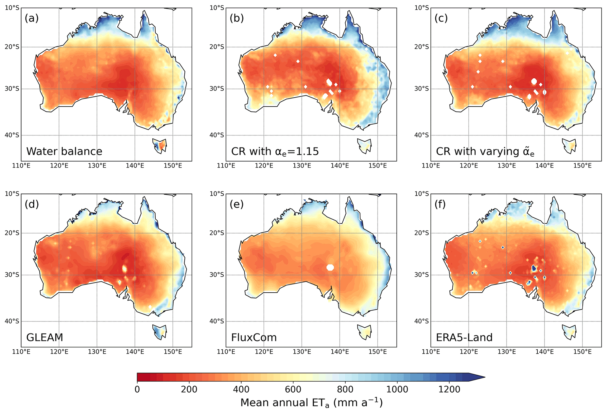
Figure 7Distributions of (a) the mean annual water-balance ETwb for 1998–2014 and the predictions by (b) CR with αe=1.15, (c) CR with spatially varying , (d) GLEAM, (e) FluxCom, and (f) ERA5-Land.
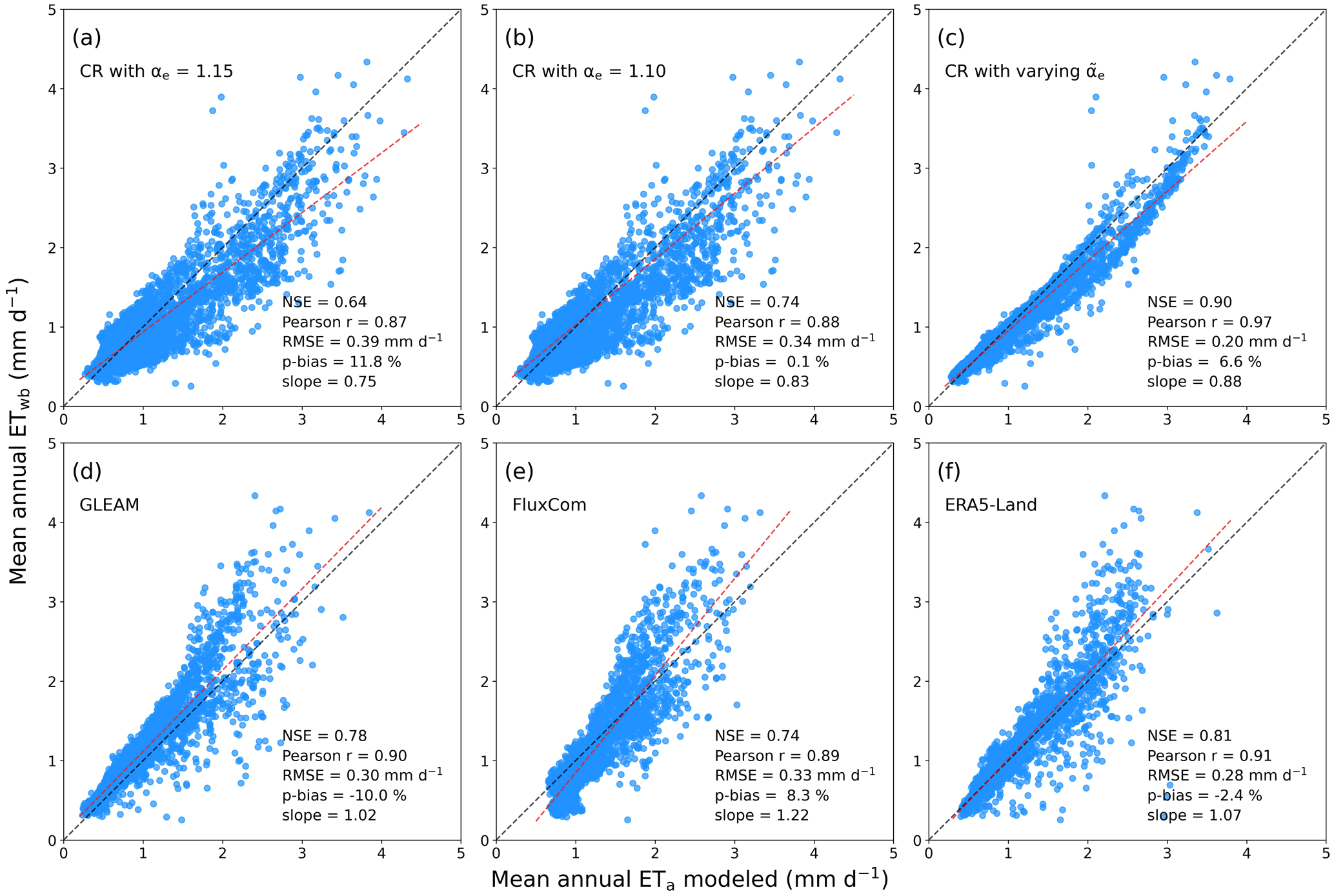
Figure 8Scatter plots between the mean annual ETwb for 1998–2014 at and the predictions by (a) CR with αe=1.15, (b) CR with αe=1.10, (c) CR with spatially varying , (d) GLEAM, (e) FluxCom, and (f) ERA5-Land.
In Crago and Qualls (2018), the optimal αe for the linear CR of Crago et al. (2016) varied largely between 1.00 and 1.43. This point-scale experiment has already suggested that a constant αe is unlikely suitable for definitive CRs to predict ETa in Australia. The ratio between the aerodynamic and the radiation components of ETw is evidently affected by the heat entrainment from the top of the boundary layer (Baldocchi et al., 2016), the dissimilarity between heat and water vapor sources (Assouline et al., 2016), the large-scale synoptic changes (Guo et al., 2015), and the horizontal advection of dry-air mass (Jury and Tanner, 1975). More recently, Han et al. (2021) proved the nonlinear dependence of ETw on ETeq, and Yang and Roderick (2019) showed αe changing with Rn over ocean surfaces. Hence, the constant αe assumption underpinning the calibration-free CR is counterintuitive to the theoretical and empirical evidence. Although Ma et al. (2021) found some global applicability of the calibration-free CR, its performance remains unknown in most of the Australian surfaces and in many ungauged basins over the world.
Since ETa plays a pivotal role in the terrestrial water and energy balances, the partitioning of Rn into the latent and the sensible heat fluxes cannot be independent of the partitioning of P into ETa and Q. On a mean annual scale, P and ETw are the major determinants of the P partitioning, and thus the parameter αe might not be independent of P. Given the large variability of P, assuming a fixed αe across a continental area may introduce considerable biases to CR ETa estimates. Thus, discarding available P data may not be a good choice when predicting ETa by the CR method in ungauged areas. It is noteworthy that Φ dominantly explained the spatial variation of the mean annual x of the 71 CAMELS basins, and the values conditioned by local climates were of a large spatial variation. This suggests that the CR with a constant αe may produce unreliable ETa estimates in ungauged locations.
Nonetheless, the low performance with a constant αe does not indicate that the CR method underperforms the sophisticated ETa models. The simple polynomial CR seemed to outperform the advanced the advanced physical, machine-learning, and land surface models, when its parameter was conditioned by local climates. The proposed CR–Budyko framework enabled us to regionalize the optimal αe for the CR method from gauged basins to ungauged locations in an empirical manner. It should be highlighted that the CR with spatially varying produced much smaller residual variance than the three advanced models.
4.2 Remaining issues and caveats
In seven Australian eddy-covariance flux towers, Crago et al. (2022) found that the optimal αe for the polynomial CR was 1.35 for predicting daily ETa in the dimensionless form (i.e., . However, it was increased to 1.42, 1.45, 1.47, and 1.50 to simulate the dimensional latent heat fluxes at daily, weekly, monthly, and annual timescales, respectively. This implies that the timescale would largely affect the optimal αe for the definitive CRs. Though the stationary Budyko equation can become a constraint at a mean-annual scale, how to capture the scale dependence of αe is a remaining question.
Further questions can arise as to how to quantify ETp and Epmax. For example, the αe values from ETp with the Rome wind function rely upon an unrealistic assumption that the aerodynamic resistance on a vegetated surface is equivalent to that of an open-water surface. It is still unknown if this assumption is practically valid because the Penman equation with the Rome wind function may result in unrealistically high ETp, even on a large wet area (McMahon et al., 2013). Given the importance of the aerodynamic resistance in modulating surface temperature (Chen et al., 2020), ignoring its variability may become a significant error source for the CR method at both annual and subannual timescales.
In addition, there are some caveats in our case study. We employed the meteorological data different from those used in Ma et al. (2021). The ERA5-Land dataset is a downscaled version of the ERA5 data (Hersbach et al., 2020) by which Ma et al. (2021) predicted ETa globally. Ma et al. (2021) incorporated remotely sensed albedo and emissivity together with a correction factor when calculating Rn, whereas we used the sum of the ERA5-Land latent and sensible heat fluxes. Those input differences may lead to differences in CR ETa estimates.
The gridded GRUN Q, too, has some uncertainty sources, though it is the ensemble of many runoff simulations from 21 different atmospheric forcing inputs. In the machine-leaning process by Ghiggi et al. (2021), some Q observations affected by human activities (e.g., dam regulation and return flows from groundwater abstraction) might not be excluded, potentially disrupting the empirical relationship between atmospheric forcing and natural flows. In addition, the uncertainty of SILO P might be non-negligible in areas with limited weather stations and in mountainous areas (Fu et al., 2022). Though we reduced the potential biases of the gridded P and Q datasets by temporal averaging, the grid-scale ETwb estimates should be treated as plausible values rather than exact observations.
Via a case study in Australia, we showed that the polynomial CR by Szilagyi et al. (2017) is unlikely to perform well when local climate conditions are neglected. The assumption of a constant Priestley–Taylor coefficient cannot reflect the long-term water balance; thereby, CR ETa estimates can be biased. We resolved this problem by conditioning the CR with the traditional Budyko equation, and it allowed for a reasonable determination of the essential parameter in ungauged locations. The following conclusions are worth emphasizing:
-
The constant Priestley–Taylor coefficient transferred from fractional wet locations could make the CR method perform poorly in closing the local water balance. The unrealistic assumption could make the CR method underperform the advanced physical, machine-learning, and land surface models.
-
The Budyko framework can play a role in determining the degree of ETp adjustment at the mean annual scale. It allows for upscaling of the Priestley–Taylor coefficients from gauged to ungauged locations.
-
The Priestley–Taylor coefficients conditioned by local climates made the CR better close the basin-scale water balance. The spatially varying Priestley–Taylor coefficients seemed to make the CR method outperform the advanced ETa models.
The Python scripts that implement the CR method are available upon request from the lead author (daeha.kim@jbnu.ac.kr).
All the datasets used in this study are publicly available. ERA5-Land reanalysis datasets are available for download at https://cds.climate.copernicus.eu/cdsapp#!/dataset/reanalysis-era5-land-monthly-means?tab=overview (last access: 10 December 2021; Muñoz-Sabater et al., 2021). The Australian edition of the Catchment Attributes and Meteorology for Large sample Studies is at https://doi.org/10.1594/PANGAEA.921850 (last access: 14 March 2022; Fowler et al., 2021). FLUXNET2015 data are readily available from the FLUXNET-Fluxdata Portal at https://fluxnet.org/data/fluxnet2015-dataset/ (last access: 1 July 2021). The GRUN ENSEMBLE can be accessed at https://figshare.com/articles/dataset/G-RUN_ENSEMBLE/12794075 (1 October 2021; Ghiggi et al., 2021). SILO P data are provided by the Queensland Government at https://www.longpaddock.qld.gov.au/silo/gridded-data/ (last access: 1 June 2021). The GLEAM is available for download at https://www.gleam.eu/ (last access: last access: 3 June 2020; Martens et al., 2017), and the FluxCom is given at http://www.fluxcom.org/EF-Download/ (last access: 18 March 2019; Jung et al., 2019).
DK, MC, and JAC organized this study together. DK built the research framework, simulated ETa with the CR method, and drafted the manuscript. JAC processed the modeled ETa datasets and reviewed the draft, and MC actively participated in discussing the results.
The contact author has declared that neither of the authors has any competing interests.
Publisher’s note: Copernicus Publications remains neutral with regard to jurisdictional claims in published maps and institutional affiliations.
This work was supported by the Korea Environmental Industry & Technology Institute (KEITI) through the Wetland Ecosystem Value Evaluation and Carbon Absorption Value Promotion Technology Development Project, funded by the Korea Ministry of Environment (MOE) (2022003640001). This work was supported by the National Research Foundation of Korea (NRF) grant, funded by the Korea government (MSIT) (NRF-2022R1A2C2010266).
This research has been jointly supported by the KEITI of MOE (grant no. 2022003640001) and the NRF of MSIT (grant no. NRF-2022R1A2C2010266).
This paper was edited by Adriaan J. (Ryan) Teuling and reviewed by two anonymous referees.
Allen, R. G., Pereira, L. S., Raes, D., and Smith, M.: Crop Evapotranspiration: Guidelines for Computing Crop Water Requirements, Irrigation and Drainage Paper 56, Food and Agriculture Organization of the United Nations: Rome, Italy, http://www.fao.org/3/x0490e/x0490e00.htm (last access: 10 June 2021), ISBN 92-5-104219-5, 1998.
Anayah, F. M. and Kaluarachchi, J. J.: Improving the complementary methods to estimate evapotranspiration under diverse climatic and physical conditions, Hydrol. Earth Syst. Sci., 18, 2049–2064, https://doi.org/10.5194/hess-18-2049-2014, 2014.
Assouline, S., Li, D., Tyler, S., Tanny, J., Cohen, S., Bou-Zeid, E., Parlange, M., and Katul, G. G.: On the variability of the Priestley-Taylor coefficient over water bodies, Water Resour. Res., 52, 150–163, https://doi.org/10.1002/2015wr017504, 2016.
Baldocchi, D. D.: How eddy covariance flux measurements have contributed to our understanding of Global Change Biology, Glob. Change Biol., 26, 242–260, https://doi.org/10.1111/gcb.14807, 2020.
Baldocchi, D., Knox, S., Dronova, I., Verfaillie, J., Oikawa, P., Sturtevant, C., Matthes, J. M., and Detto, M.: The impact of expanding flooded land area on the annual evaporation of rice, Agr. Forest Meteorol. 223, 181–193, https://doi.org/10.1016/j.agrformet.2016.04.001, 2016.
Balsamo, G., Albergel, C., Beljaars, A., Boussetta, S., Brun, E., Cloke, H., Dee, D., Dutra, E., Muñoz-Sabater, J., Pappenberger, F., de Rosnay, P., Stockdale, T., and Vitart, F.: ERA-Interim/Land: a global land surface reanalysis data set, Hydrol. Earth Syst. Sci., 19, 389–407, https://doi.org/10.5194/hess-19-389-2015, 2015.
Bouchet, R. J.: Evapotranspiration re'elle et potentielle, signification climatique, in: General Assembly Berkeley, Int. Assoc. Sci. Hydrol., Gentbrugge, Belgium, Publ. No. 62, 134–142, 1963.
Brutsaert, W., Cheng, L., and Zhang, L.: Spatial distribution of global landscape evaporation in the early twenty-first century by means of a generalized complementary approach, J. Hydrometeorol., 21, 287–298, https://doi.org/10.1175/JHM-D-19-0208.1, 2020.
Brutsaert, W., Li, W., Takahashi, A., Hiyama, T., Zhang, L., and Liu, W.: Nonlinear advection-aridity method for landscape evaporation and its application during the growing season in the southern Loess Plateau of the Yellow River basin, Water Resour. Res., 53, 270–282. https://doi.org/10.1002/2016WR019472, 2017.
Brutsaert, W.: A generalized complementary principle with physical constraints for land-surface evaporation, Water Resour. Res., 51, 8087–8093, https://doi.org/10.1002/2015WR017720, 2015.
Carmona, A. M., Poveda, G., Sivapalan, M., Vallejo-Bernal, S. M., and Bustamante, E.: A scaling approach to Budyko's framework and the complementary relationship of evapotranspiration in humid environments: case study of the Amazon River basin, Hydrol. Earth Syst. Sci., 20, 589–603, https://doi.org/10.5194/hess-20-589-2016, 2016.
Chen, C., Li, D., Li, Y., Piao, S., Wang, X., Huang, M., Gentine, P., Nemani, R. R., and Myneni, R. B.: Biophysical impacts of Earth greening largely controlled by aerodynamic resistance, Sci. Adv., 6, eabb1981, https://doi.org/10.1126/sciadv.abb1981, 2020.
Chen, X. and Buchberger, S. G.: Exploring the relationships between warm-season precipitation, potential evaporation, and “apparent” potential evaporation at site scale, Hydrol. Earth Syst. Sci., 22, 4535–4545, https://doi.org/10.5194/hess-22-4535-2018, 2018.
Crago, R. D. and Qualls, R. J.: A graphical interpretation of the rescaled complementary relationship for evapotranspiration. Water Resour. Res., 57, e2020WR028299, https://doi.org/10.1029/2020WR028299, 2021.
Crago, R. D., and Qualls, R. J.: Evaluation of the generalized and rescaled complementary evaporation relationships, Water Resour. Res., 54, 8086–8102, https://doi.org/10.1029/2018WR023401, 2018.
Crago, R. D. and Qualls, R. J.: The value of intuitive concepts in evaporation research, Water Resour. Res., 49, 6100–6104, https://doi.org/10.1002/wrcr.20420, 2013.
Crago, R. D., Qualls, R., and Szilagyi, J.: Complementary Relationship for evaporation performance at different spatial and temporal scales, J. Hydrol., 608, 127575, https://doi.org/10.1016/j.jhydrol.2022.127575, 2022.
Crago, R. and Crowley, R.: Complementary relationships for near-instantaneous evaporation, J. Hydrol., 300, 199–211, https://doi.org/10.1016/j.jhydrol.2004.06.002, 2005.
Crago, R., Szilagyi, J., Qualls, R., and Huntington, J.: Rescaling the complementary relationship for land surface evaporation, Water Resour. Res., 52, 8461–8471, https://doi.org/10.1002/2016WR019753, 2016.
Fowler, K. J. A., Acharya, S. C., Addor, N., Chou, C., and Peel, M. C.: CAMELS-AUS: hydrometeorological time series and landscape attributes for 222 catchments in Australia, [data set], Earth Syst. Sci. Data, 13, 3847–3867, https://doi.org/10.5194/essd-13-3847-2021, 2021.
Fu, B. P.: On the calculation of evaporation from land surface. Scientia Atmospherica Sinica, 1, 23–31, 1981.
Fu, G., Barron, O., Charles, S. P., Donn, M. J., Van Niel, T. G., and Hodgson, G.: Uncertainty of gridded precipitation at local and continent scales: A direct comparison of rainfall from SILO and AWAP in Australia, Asia-Pacific J. Atmos. Sci., 58, 471–488, https://doi.org/10.1007/s13143-022-00267-4, 2022.
Ghiggi, G., Humphrey, V., Seneviratne, S. I., and Gudmundsson, L.: G-RUN ENSEMBLE: A multi-forcing observation-based global runoff reanalysis, [data set], Water Resour. Res., 57, e2020WR028787, https://doi.org/10.1029/2020WR028787, 2021.
Glenn, E.P., Doody, T.M., Guerschman, J.P., Huete, A.R., King, E.A., McVicar, T.R., Van Dijk, A.I.J.M., Van Niel, T.G., Yebra, M., and Zhang, Y.: Actual evapotranspiration estimation by ground and remote sensing methods: the Australian experience, Hydrol. Proc., 25, 4103–4116, https://doi.org/10.1002/hyp.8391, 2011
Guimberteau, M., Zhu, D., Maignan, F., Huang, Y., Yue, C., Dantec-Nédélec, S., Ottlé, C., Jornet-Puig, A., Bastos, A., Laurent, P., Goll, D., Bowring, S., Chang, J., Guenet, B., Tifafi, M., Peng, S., Krinner, G., Ducharne, A., Wang, F., Wang, T., Wang, X., Wang, Y., Yin, Z., Lauerwald, R., Joetzjer, E., Qiu, C., Kim, H., and Ciais, P.: ORCHIDEE-MICT (v8.4.1), a land surface model for the high latitudes: model description and validation, Geosci. Model Dev., 11, 121–163, https://doi.org/10.5194/gmd-11-121-2018, 2018.
Guo, X., Liu, H., and Yang, K.: On the application of the Priestley–Taylor relation on sub-daily time scales, Bound. Lay. Meteorol., 156, 489–499, https://doi.org/10.1007/s10546-015-0031-y, 2015.
Hagedorn, F., Gavazov, K., and Alexander, J. M.: Above- and belowground linkages shape responses of mountain vegetation to climate change, Science, 365, 1119–1123, https://doi.org/10.1126/science.aax4737, 2019.
Han, S. and Tian, F.: Derivation of a sigmoid generalized complementary function for evaporation with physical constraints, Water Resour. Res., 54, 5050–5068, https://doi.org/10.1029/2017WR021755, 2018.
Han, S., Tian, F., Wang, W., and Wang, L.: Sigmoid generalized complementary equation for evaporation over wet surfaces: A nonlinear modification of the Priestley-Taylor equation, Water Resour. Res., 57, e2020WR028737, https://doi.org/10.1029/2020WR028737, 2021.
Haverd, V., Smith, B., Nieradzik, L., Briggs, P. R., Woodgate, W., Trudinger, C. M., Canadell, J. G., and Cuntz, M.: A new version of the CABLE land surface model (Subversion revision r4601) incorporating land use and land cover change, woody vegetation demography, and a novel optimisation-based approach to plant coordination of photosynthesis, Geosci. Model Dev., 11, 2995–3026, https://doi.org/10.5194/gmd-11-2995-2018, 2018.
Hersbach, H., Bell, B., Berrisford, P., Hirahara, S., Horányi, A., Muñoz-Sabater, J., Nicolas, J., Peubey, C., Radu, R., Schepers, D., Simmons, A., Soci, C., Abdalla, S., Abellan, X., Balsamo, G., Bechtold, P., Biavati, G., Bidlot, J., Bonavita, M., De Chiara, G., Dahlgren, P., Dee, D., Diamantakis, M., Dragani, R., Flemming, J., Forbes, R., Fuentes, M., Geer, A., Haimberger, L., Healy, S., Hogan, R. J., Hólm, E., Janisková, M., Keeley, S., Laloyaux, P., Lopez, P., Lupu, C., Radnoti, G., de Rosnay, P., Rozum, I., Vamborg, F., Villaume, S., and Thépaut, J.-N.: The ERA5 global reanalysis, Q. J. R. Meteorol. Soc. 146, 1999–2049. https://doi.org/10.1002/qj.3803, 2020.
Hobbins, M. T., Ramírez, J. A., and Brown, T. C.: Trends in pan evaporation and actual evapotranspiration across the conterminous U.S.: Paradoxical or complementary? Geophys. Res. Lett., 31, L13503, https://doi.org/10.1029/2004GL019846, 2004.
Huntington, J. L., Szilagyi, J., Tyler, S. W., and Pohll, G. M.: Evaluating the complementary relationship for estimating evapotranspiration from arid shrublands, Water Resour. Res., 47, W05533, https://doi.org/10.1029/2010WR009874, 2011.
Jasechko, S.: Plants turn on the tap, Nat. Clim. Change, 8, 562–563, https://doi.org/10.1038/s41558-018-0212-z, 2018.
Jung, M., Koirala, S., Weber, U., Ichii, K., Gans, F., Camps-Valls, G., Papale, D., Schwalm, C., Tramontana, G., and Reichstein, M: The FLUXCOM ensemble of global land-atmosphere energy fluxes, [data set], Sci. data, 6, 74, https://doi.org/10.1038/s41597-019-0076-8, 2019.
Jury, W. and Tanner, C.: Advection modification of the Priestley and Taylor evapotranspiration formula, Agron. J., 67, 840–842, https://doi.org/10.2134/agronj1975.000219620, 1975.
Kahler, D. M. and Brutsaert, W.: Complementary relationship between daily evaporation in the environment and pan evaporation, Water Resour. Res., 42, W05413, https://doi.org/10.1029/2005WR004541, 2006.
Kim, D., and Chun, J. A.: Revisiting a two-parameter Budyko equation with the complementary evaporation principle for proper consideration of surface energy balance, Water Resour. Res., 57, e2021WR030838, https://doi.org/10.1029/2021WR030838, 2021.
Kim, D., Ha, K.-J., and Yeo, J.-H.: New drought projections over East Asia using evapotranspiration deficits from the CMIP6 warming scenarios, Earths Future, 9, e2020EF001697, https://doi.org/10.1029/2020EF001697, 2021.
Kim, D., Lee, W.-S., Kim, S. T., and Chun, J. A.: Historical drought assessment over the contiguous United States using the generalized complementary principle of evapotranspiration, Water Resour. Res., 55, 6244–6267, https://doi.org/10.1029/2019WR024991, 2019.
Kyatengerwa, C., Kim, D., and Choi, M.: A national-scale drought assessment in Uganda based on evapotranspiration deficits from the Bouchet hypothesis, J. Hydrol., 500, 124348, https://doi.org/10.1016/j.jhydrol.2019.124348, 2020.
Lhomme, J.-P. and Moussa, R.: Matching the Budyko functions with the complementary evaporation relationship: consequences for the drying power of the air and the Priestley–Taylor coefficient, Hydrol. Earth Syst. Sci., 20, 4857–4865, https://doi.org/10.5194/hess-20-4857-2016, 2016.
Ma, N. and Szilagyi, J.: The CR of evaporation: a calibration-free diagnostic and benchmarking tool for large-scale terrestrial evapotranspiration modeling. Water Resour. Res., 55, 7246–7274, https://doi.org/10.1029/2019WR024867, 2019.
Ma, N., Szilagyi, J., and Zhang, Y.: Calibration-free complementary relationship estimates terrestrial evapotranspiration globally, Water Resour. Res., 57, e2021WR029691, https://doi.org/10.1029/2021WR029691, 2021.
Ma, N., Szilagyi, J., Zhang, Y., and Liu, W.: Complementary-relationship-based modeling of terrestrial evapotranspiration across China during 1982–2012: validations and spatiotemporal analyses, J. Geophys. Res. Atmos., 124, 4326–4351, https://doi.org/10.1029/2018JD029850, 2019.
Martens, B., Miralles, D. G., Lievens, H., van der Schalie, R., de Jeu, R. A. M., Fernández-Prieto, D., Beck, H. E., Dorigo, W. A., and Verhoest, N. E. C.: GLEAM v3: satellite-based land evaporation and root-zone soil moisture, [data set], Geosci. Model Dev., 10, 1903–1925, https://doi.org/10.5194/gmd-10-1903-2017, 2017.
Martens, B., Schumacher, D. L., Wouters, H., Muñoz-Sabater, J., Verhoest, N. E. C., and Miralles, D. G.: Evaluating the land-surface energy partitioning in ERA5, Geosci. Model Dev., 13, 4159–4181, https://doi.org/10.5194/gmd-13-4159-2020, 2020.
McMahon, T. A., Peel, M. C., Lowe, L., Srikanthan, R., and McVicar, T. R.: Estimating actual, potential, reference crop and pan evaporation using standard meteorological data: a pragmatic synthesis, Hydrol. Earth Syst. Sci., 17, 1331–1363, https://doi.org/10.5194/hess-17-1331-2013, 2013.
Mekonnen, Z. A., Riley, W. J., Randerson, J. T., Grant, R. F., and Rogers, B. M.: Expansion of high-latitude deciduous forests driven by interactions between climate warming and fire, Nat. Plants, 5, 952–958, https://doi.org/10.1038/s41477-019-0495-8, 2019.
Mianabadi, A., Davary, K., Pourreza-Bilondi, M., and Coenders-Gerrits, A. M. J.: Budyko framework: Towards non-steady state conditions, J. Hydrol., 588, 125089, https://doi.org/10.1016/j.jhydrol.2020.125089, 2020.
Miralles, D., G., Teuling, A., J. van Heerwaarden, C. C., and de Arellano, J. V.-G.: Mega-heatwave temperatures due to combined soil desiccation and atmospheric heat accumulation, Nat. Geosci., 7, 345–349, https://doi.org/10.1038/ngeo2141, 2014.
Mueller, B. and Seneviratne, S. I.: Hot days induced by precipitation deficits at the global scale, P. Natl. Acad. Sci. USA, 109, 12398–12403, https://doi.org/10.1073/pnas.1204330109, 2012.
Muñoz-Sabater, J., Dutra, E., Agustí-Panareda, A., Albergel, C., Arduini, G., Balsamo, G., Boussetta, S., Choulga, M., Harrigan, S., Hersbach, H., Martens, B., Miralles, D. G., Piles, M., Rodríguez-Fernández, N. J., Zsoter, E., Buontempo, C., and Thépaut, J.-N.: ERA5-Land: a state-of-the-art global reanalysis dataset for land applications, [data set], Earth Syst. Sci. Data, 13, 4349–4383, https://doi.org/10.5194/essd-13-4349-2021, 2021.
Novick, K. A., Biederman, J. A., Desai, A. R., Litvak, M. E., Moore, D. J. P., Scott, R. L., and Torn, M. S.: The AmeriFlux network: A coalition of the willing, Agr. Forest Meteorol., 249, 444–456, https://doi.org/10.1016/j.agrformet.2017.10.00, 2018.
Pan, S., Pan, N., Tian, H., Friedlingstein, P., Sitch, S., Shi, H., Arora, V. K., Haverd, V., Jain, A. K., Kato, E., Lienert, S., Lombardozzi, D., Nabel, J. E. M. S., Ottlé, C., Poulter, B., Zaehle, S., and Running, S. W.: Evaluation of global terrestrial evapotranspiration using state-of-the-art approaches in remote sensing, machine learning and land surface modeling, Hydrol. Earth Syst. Sci., 24, 1485–1509, https://doi.org/10.5194/hess-24-1485-2020, 2020.
Pareek, A., Dhankher, O. P., and Foyer, C. H.: Mitigating the impact of climate change on plant productivity and ecosystem sustainability, J. Exp. Bot., 71, 451–456, https://doi.org/10.1093/jxb/erz518, 2020.
Parlange, M. B. and Katul, G. G.: Estimation of the diurnal variation of potential evaporation from a wet bare soil surface, J. Hydrol., 132, 71–89, https://doi.org/10.1016/0022-1694(92)90173-s, 1992.Qualls and Crago, 2020
Penman, H. L.: Natural evaporation from open water, bares soil, and grass, P. Roy. Soc. A, 193, 120–146. https://doi.org/10.1098/rspa.1948.0037, 1948.
Priestley, C. H. and Taylor, R. J.: On the assessment of surface heat flux and evaporation using large-scale parameters, Mon. Weather Rev., 100, 81–92, 1972.
Ramírez, J. A., Hobbins, M. T., and Brown, T. C.: Observational evidence of the complementary relationship in regional evaporation lends strong support for Bouchet's hypothesis, Geophys. Res. Lett., 32, L15401, https://doi.org/10.1029/2005GL023549, 2005.
Rodriguez-Iturbe, I.: Ecohydrology: A hydrologic perspective of climate-soil-vegetation dynamies, Water Resour. Res., 36, 3–9, https://doi.org/10.1029/1999WR900210, 2000.
Schlosser, C. A. and Gao, X.: Assessing evapotranspiration estimates from the second global soil wetness project (GSWP-2) simulations, J. Hydrometeorol., 11, 880–897, https://doi.org/10.1175/2010jhm1203.1, 2010.
Schumacher, D.L., Keune, J., van Heerwaarden, C.C., de Alrellano, J. V., Teuling, A. J., and Miralles, D. G.: Amplification of mega-heatwaves through heat torrents fuelled by upwind drought, Nat. Geosci., 12, 712–717, https://doi.org/10.1038/s41561-019-0431-6, 2019.
Sun, Q., Miao, C., Duan, Q., Ashouri, H., Sorooshian, S., and Hsu, K.-L.: A review of global precipitation datasets: Data sources, estimation, and intercomparisons, Rev. Geophys., 56, 79–107, https://doi.org/10.1002/2017rg000574, 2018.
Szilagyi, J. and Schepers, A.: Coupled heat and vapor transport: The thermostat effect of a freely evaporating land surface, Geophys. Res. Lett., 41, 435–441, https://doi.org/10.1002/2013gl058979, 2014.
Szilagyi, J., Crago, R., and Qualls, R.: A calibration-free formulation of the complementary relationship of evaporation for continental-scale hydrology, J. Geophys. Res.-Atmos., 122, 264–278, https://doi.org/10.1002/2016jd025611, 2017.
Szilagyi, J.: On the thermodynamics foundations of the complementary relationship of evaporation, J. Hydrol., 593, 125916, https://doi.org/10.1016/j.jhydrol.2020.125916, 2021.
Tramontana, G., Jung, M., Schwalm, C. R., Ichii, K., Camps-Valls, G., Ráduly, B., Reichstein, M., Arain, M. A., Cescatti, A., Kiely, G., Merbold, L., Serrano-Ortiz, P., Sickert, S., Wolf, S., and Papale, D.: Predicting carbon dioxide and energy fluxes across global FLUXNET sites with regression algorithms, Biogeosciences, 13, 4291–4313, https://doi.org/10.5194/bg-13-4291-2016, 2016.
Trenberth, K. E., Fasullo, J. T., and Kiehl, J.: Earth's global energy budget, B. Am. Meteorol. Soc., 90, 311–324, https://doi.org/10.1175/2008BAMS2634.1, 2009.
Trenberth, K. E., Smith, L., Qian, T., Dai, A., and Fasullo, J.: Estimates of the global water Budget and its annual cycle using observational and model data, J. Hydrometeorol., 8, 758–769, https://doi.org/10.1175/JHM600.1, 2007.
Wang, W., Xiao, W., Cao, C., Gao, Z., Hu, Z., Liu, S., Shen, S., Wang, L., Xiao, Q., Xu, J., Yang D., and Lee X.: Temporal and spatial variations in radiation and energy balance across a large freshwater lake in China, J. Hydrol., 511, 811–824, https://doi.org/10.1016/j.jhydrol.2014.02.012, 2014.
Yang, H., Yang, D., Lei, Z., and Sun, F.: New analytical derivation of the mean annual water balance equation, Water Resour. Res., 44, W03410, https://doi.org/10.1029/2007WR006135, 2008.
Yang, Y. and Roderick, M. L.: Radiation, surface temperature and evaporation over wet surfaces, Q. J. R. Meteorol. Soc., 145, 1118–1129, https://doi.org/10.1002/qj.3481, 2019.
Zhang, K., Zhu, G., Ma, J., Yang, Y., Shang, S., and Gu, C.: Parameter analysis and estimates for the MODIS evapotranspiration algorithm and multiscale verification, Water Resour. Res., 55, 2211–2231, https://doi.org/10.1029/2018wr023485, 2019.
Zhang, L. and Brutsaert, W.: Blending the evaporation precipitation ratio with the complementary principle function for the prediction of evaporation, Water Resour. Res., 57, e2021WR029729, https://doi.org/10.1029/2021WR029729, 2021
Zhang, Y., Peña-Arancibia, J. L., McVicar, T. R., Chiew, F. H., Vaze, J., Liu, C., Lu, X., Zheng, H., Wang, Y., and Liu, Y. Y.: Multi-decadal trends in global terrestrial evapotranspiration and its components, Sci. Rep., 6, 19124, https://doi.org/10.1038/srep19124, 2016.
Zhou, S., Williams, A. P., Berg, A. M., Cook, B. I., Zhang, Y., Hagemann, S., Lorenz, R., Seneviratne, S. I., and Gentine, P.: Land–atmosphere feedbacks exacerbate concurrent soil drought and atmospheric aridity, P. Natl. Acad. Sci. USA, 116, 18848–18853, https://doi.org/10.1073/pnas.1904955116, 2019.