the Creative Commons Attribution 4.0 License.
the Creative Commons Attribution 4.0 License.
 | 25 Nov 2022
Monitoring the extreme flood events in the Yangtze River basin based on GRACE and GRACE-FO satellite data
Jingkai Xie
Hongjie Yu
Yan Huang
Yuxue Guo
Gravity Recovery and Climate Experiment (GRACE) and its successor GRACE Follow-on (GRACE-FO) satellite provide terrestrial water storage anomaly (TWSA) estimates globally that can be used to monitor flood in various regions at monthly intervals. However, the coarse temporal resolution of GRACE and GRACE-FO satellite data has been limiting their applications at finer temporal scales. In this study, TWSA estimates have been reconstructed and then temporally downscaled into daily values based on three different learning-based models, namely a multi-layer perceptron (MLP) model, a long-short term memory (LSTM) model and a multiple linear regression (MLR) model. Furthermore, a new index incorporating temporally downscaled TWSA estimates combined with daily average precipitation anomalies is proposed to monitor the severe flood events at sub-monthly timescales for the Yangtze River basin (YRB), China. The results indicated that (1) the MLP model shows the best performance in reconstructing the monthly TWSA with root mean square error (RMSE) = 10.9 mm per month and Nash–Sutcliffe efficiency (NSE) = 0.89 during the validation period; (2) the MLP model can be useful in temporally downscaling monthly TWSA estimates into daily values; (3) the proposed normalized daily flood potential index (NDFPI) facilitates robust and reliable characterization of severe flood events at sub-monthly timescales; (4) the flood events can be monitored by the proposed NDFPI earlier than traditional streamflow observations with respect to the YRB and its individual subbasins. All these findings can provide new opportunities for applying GRACE and GRACE-FO satellite data to investigations of sub-monthly signals and have important implications for flood hazard prevention and mitigation in the study region.
- Article
(6347 KB) - Full-text XML
-
Supplement
(1037 KB) - BibTeX
- EndNote


Extreme floods, as one of the most destructive natural hazards, not only cause lots of casualties in China and around the world, but also have considerable wider and adverse economic consequences (Dottori et al., 2018). According to the report published by the United Nations Office for Disaster Risk Reduction (UNDRR), the total economic loss induced by floods is up to USD 651 billion worldwide from 2000 to 2019 (https://www.undrr.org/publication/human-cost-disasters-overview-last-20-years-2000-2019, last access: 17 November 2022). Meanwhile, floods are projected to become more frequent and extreme under global warming as it can substantially amplify the water-holding capacity of the air and increase the occurrence of extreme precipitation events (Slater and Villarini, 2016). Therefore, monitoring extreme flood events has long been a hot topic for hydrologists and decision makers around the world (Tanoue et al., 2020; Tellman et al., 2021).
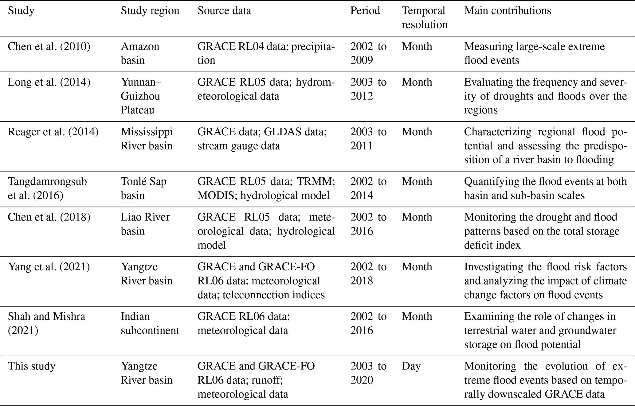
Contrary to traditionally ground-based observations or hydrological models, the launches of Gravity Recovery and Climate Experiment (GRACE) twin satellites in 2002 and its successor GRACE Follow-on (GRACE-FO) satellites in 2018 can provide a new methodology for retrieving terrestrial water storage anomalies (TWSAs) in real time globally by measuring temporal variations in Earth's gravity field (Ahmed et al., 2021; Tapley et al., 2004). The TWSA derived from GRACE and GRACE-FO satellites comprises all the surface and subsurface water over land, which can be used to monitor the hydrologic variations in response to extreme weather events (Li et al., 2022; Xie et al., 2019a). In this case, GRACE and GRACE-FO observations have been widely applied to assess the potential flood risks for a specific region. For example, Reager and Famiglietti (2009) proposed a flood potential index estimated using monthly average precipitation anomalies and GRACE-derived TWSAs to characterize the potential flood risks from regional to global scales. Xiong et al. (2021a) developed a novel integrated flood potential index by linking the flood potential index derived from six GRACE products based on a copula function, which was further used to identify and characterize the floods with different intensities over the study region. A summary of relevant literature on detecting extreme flood events using GRACE and GRACE-FO data has been listed in Table 1.
Table 1A summary of relevant literature on monitoring extreme flood events using GRACE and GRACE-FO data. GRACE: Gravity Recovery and Climate Experiment mission. GRACE-FO: Gravity Recovery and Climate Experiment Follow-On mission. GLDAS: Global Land Data Assimilation system. TRMM: Tropical Rainfall Measuring Mission. MODIS: Moderate-Resolution Imaging Spectroradiometer.
Previous studies have clearly indicated that the proposed indices using GRACE and GRACE-FO data can better reflect the evolution of flood events than traditional indices, such as standardized precipitation index (SPI) and standardized precipitation evapotranspiration index (SPEI), because the GRACE and GRACE-FO observations can measure the vertically integrated water storage over regions (Yan et al., 2021; Yin and Park, 2021). However, all these studies mainly focus on detecting the extreme flood events at monthly intervals, while monitoring the flood events and its hydrological impacts at finer temporal scales remains a major challenge due to the coarse temporal resolution (i.e., monthly) of GRACE and GRACE-FO data. To date, very few studies have paid attention to monitor flood events at sub-monthly timescales using GRACE data. Given the rapid occurrence and evolution of some extreme events within a short period, there is a great need to monitor the flood events at a finer temporal resolution (e.g., day), which has important implications for better understanding the mechanisms of extreme flood events in the Yangtze River basin (YRB). Therefore, we aim to downscale the TWSA estimates derived from GRACE and GRACE-FO satellite data into daily values and demonstrate its application to monitor extreme flood events at sub-monthly timescales for the YRB. The temporally downscaled TWSA data could be valuable for understanding the effects of climate change on the hydrological cycle and providing important implications of flood hazard prevention and water resource management over this region.
The YRB is one of the most important basins in China because it can provide freshwater, hydropower, food, and other ecosystem services for hundreds of millions of people. Meanwhile, the YRB has been regarded as one of the most sensitive and vulnerable regions that has suffered from severe floods due to its highly uneven rainfall pattern (Zhang et al., 2021). During the past decades, increasingly intensified human activities and climate change have substantially changed the hydrological cycle in the YRB and thus accelerated the variation of flood characteristics in this region (Fang et al., 2012; Wang et al., 2011). It has been found that both the frequency and severity of extreme flood events generally showed upward trends in the YRB in recent decades, owing to substantial changes in climate, infrastructure and land use (Huang et al., 2015; Liu et al., 2019; Yang et al., 2021; Zhang et al., 2008). For example, in the year 2020, the YRB experienced one of the most extreme flood events on record. According to data from the Ministry of Emergency Management of the People's Republic of China, a total of 38.173 million people were affected, and 27 000 houses collapsed due to the 2020 flood, with 56 deaths or disappearances and a great economic loss of USD 27.68 billion (Jia et al., 2021).
The rest of this paper is mainly organized as follows. In Sect. 2, descriptions of the study area are presented. In Sects. 3 and 4, the datasets and methods used in this study are introduced respectively. In Sect. 5, monthly TWSA estimates obtained from original GRACE and GRACE-FO satellite data are temporally downscaled into individual values at daily timescales based on the methodology proposed in this study. Meanwhile, a new index incorporating temporally downscaled TWSA estimates and daily precipitation is proposed to detect extreme flood events that occurred in the year 2020 across the YRB and its individual subbasins. Then, the discussion about the temporally downscaled GRACE and GRACE-FO satellite data and its capacity to monitor extreme flood events are presented in Sect. 6. We also explain the reasons why the new proposed index can monitor extreme flood events across the YRB in this section. Finally, we present a summary of this study in Sect. 7.
The Yangtze River (also termed as Changjiang River) is the longest river in China, with a length of about 6300 km. It originates from the Tanggula Mountains of the Qinghai–Tibetan Plateau and eventually empties into the estuary of the East China Sea after spanning 11 provinces in China (Wu et al., 2022). The YRB (90–122∘ E, 25–35∘ N) has a total drainage area of 1.81×10⁶ km2, which accounts for approximately 20 % of the total area of the mainland China. The terrain of the YRB generally decreases from west to east, with altitudes ranging from −142 to 7143 m above sea level (shown in Fig. 1). The entire YRB consists of three main parts, that is, the upper (upstream region above the Yichang station), the middle (region between the Yichang station and the Hukou station) and the lower (downstream region below the Hukou station) subbasins.
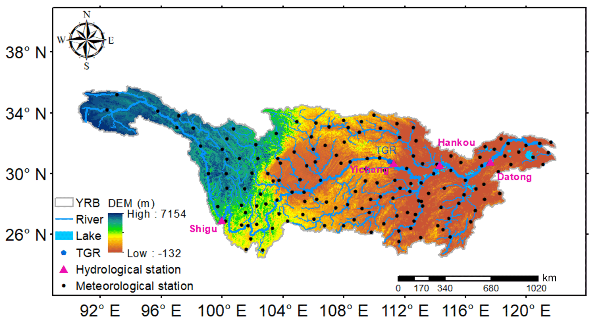
Figure 1Location of the Yangtze River basin (YRB) in China and its topography. Distribution of meteorological stations and hydrological stations is also shown in this figure. TGR: Three Gorges Reservoir. DEM: digital elevation model.
The YRB is located in typically subtropical and temperate climate zones, which is dominated by three types of monsoons, namely the Siberian northwest monsoon winds in winter and the Indian southeasterly monsoon winds and the East Asian monsoon in summer (Kong et al., 2020). According to observations from meteorological stations, the mean annual air temperature of this basin ranges from 14.4 to 15.4 ∘C, and mean annual precipitation ranges from 1049 to 1424 mm during 2003–2020. Under the joint effects of monsoon activities and seasonal motions of subtropical highs, more than 85 % of the annual precipitation occurs in the wet season from April to October, which further increases the risks of extreme floods in the middle and lower reaches of the Yangtze River (Huang et al., 2015; Yang et al., 2010). Additionally, by the end of 21st century, projections show a significant upward trend of the annual precipitation over the YRB according to the latest study (Yue et al., 2021).
The YRB is one of the most important regions in China because it accommodates approximately 33 % of China's total population (Huang et al., 2021), accounts for over 36 % China's total water resources and contributes more than 46 % of China's total gross domestic product (GDP) according to statistics collected by Yangtze River Conservancy Commission of Ministry of Water Resources. The YRB not only sustains many hydro-electrical industries, such as the Three Gorges Corporation, but also provides freshwater resources for neighboring regions to alleviate the pressure of water scarcity through the South-to-North Water Diversion Project (Long et al., 2020; Zhang et al., 2021). Furthermore, the YRB plays a critical role in flood control, crop irrigation, power generation and ecological conservation (Chao et al., 2021; L. Wang et al., 2020). More information about the location and topography of the YRB can be found in Fig. 1.
3.1 Terrestrial water storage derived from GRACE and GRACE-FO satellite data
GRACE and GRACE-FO data can provide global TWSA at monthly scales. In this study, the average of three types of GRACE and GRACE-FO solutions is estimated in order to characterize the variations of TWSA in the YRB and its individual subbasins during the period of 2003–2020, all of which are the latest versions of Release Number 06 (RL06). These products are provided by the Center for Space Research (CSR; at the University of Texas at Austin) (Save et al., 2016), the Goddard Space Flight Center (GSFC; at NASA) (Loomis et al., 2019) and the Jet Propulsion Laboratory (JPL; at NASA and California Institute of Technology, California) (Landerer et al., 2020) respectively. All these GRACE and GRACE-FO solutions represented by equivalent water thickness units (mm) are anomalies relative to the time-mean baseline during January 2004–December 2009. It should also be noteworthy that GRACE data are not available in a few months because of the problem of “battery management”. In addition, there was a gap period for 11 consecutive months from July 2017 to May 2018 between the GRACE and GRACE-FO satellites. Here we have not filled the data gaps between the two GRACE satellites with linear interpolation since it may not fully describe the seasonal variation of TWSA during these missing months. All these GRACE and GRACE-FO satellite data are available at https://podaac.jpl.nasa.gov (last access: 17 November 2022). As documented in previous studies (Long et al., 2014; Xie et al., 2022), there are slight differences between these three GRACE and GRACE-FO solutions when estimating the variation of regional TWSA. The differences between these three GRACE and GRACE-FO solutions mainly arise from the processing algorithms or constrained solutions.
3.2 Meteorological data
In this study, daily time series of precipitation and temperature from 2003–2020 are provided by the China Meteorological Administration (CMA) (http://data.cma.cn/, last access: 17 November 2022) with a total of 150 National Meteorological Observatory stations distributed in the YRB (shown in Fig. 1). Areal precipitation in the YRB and its individual subbasins at daily scales can be calculated according to the Thiessen polygon method. Monthly precipitation for regions is calculated by summing all daily values of precipitation. Meanwhile, areal temperature in the YRB and its basins at daily timescales is calculated by directly averaging the respective daily temperature from all meteorological stations over regions. Similarly, monthly temperature estimates are calculated by summing all daily values of temperature.
3.3 In situ streamflow data
From the Yangtze River Conservancy Commission of Ministry of Water Resources, daily streamflow observations during the period of 2003–2020 can be obtained at the Shigu hydrological station, the Yichang hydrological station, the Hankou hydrological station and the Datong hydrological station (shown in Fig. 1). More specifically, the Shigu station represents the outlet of the source regions of the Yangtze River basin (SYRB), the Yichang station represents the outlet of the upper regions of the Yangtze River basin (UYRB), the Hankou station represents the outlet of the upper and the middle regions of the Yangtze River basin (UMYRB), and the Datong station represents the outlet of the entire Yangtze River basin (YRB). Meanwhile, extreme flood events in the YRB and its individual subbasins during the study period can be extracted from daily time series of streamflow observed from the above hydrological stations (Tarasova et al., 2018). More details about how the extreme flood events are extracted will be described in the Sect. 4.4.
3.4 Soil moisture storage
As documented in Xie et al. (2019a), soil moisture storage (SMS), as one of critical components of terrestrial water storage, usually shows a significantly positive correlation with variations of regional TWSA. Therefore, in this study we adopt the SMS (kg m−2) with a spatial resolution of 0.25∘ × 0.25∘ from the Global Land Data Assimilation System version 2.1 (GLDAS 2.1) Noah land surface model to estimate their correlations with regional TWSA derived from the GRACE and GRACE-FO satellite data. This product can provide the simulations of SMS at four different depths of soil layers from 0 to 200 cm, that is, 0–10, 10–40, 40–100 and 100–200 cm depths per 3 h. To keep consistent with the TWSA, the original value of SMS should be transferred into soil moisture storage anomaly (SMSA) values after subtracting the time-mean baseline during the period of 2004–2009. Furthermore, the temporal resolution of original SMS derived from GLDAS 2.1 Noah land surface model can be decreased from 3 h to 1 d and 1-month composite respectively, which is consistent with the methods applied in previous studies (Mulder et al., 2015; Mohanasundaram et al., 2021; Syed et al., 2008). An overview of all datasets used in this study can be found in Table 2.
Table 2An overview of all datasets used in this study.
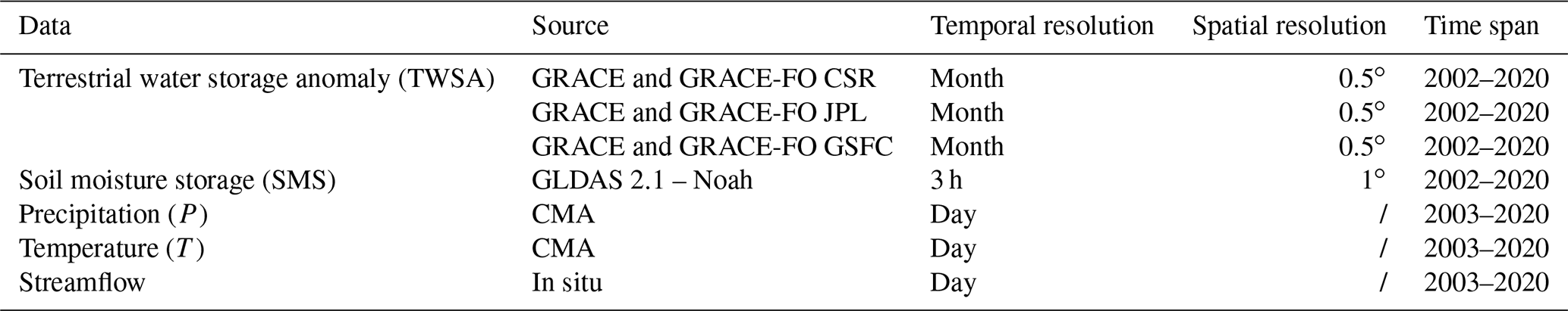
GRACE: Gravity Recovery and Climate Experiment mission. GRACE-FO: Gravity Recovery and Climate Experiment Follow-On mission. CSR: Center for Space Research. JPL: Jet Propulsion Laboratory. GSFC: Goddard Space Flight Center. GLDAS: Global Land Data Assimilation system. CMA: China Meteorological Administration.
To better monitor the extreme flood events that occurred in the YRB, monthly TWSA obtained from original GRACE and GRACE-FO satellite data are temporally downscaled into individual values at daily timescales based on the methodology proposed in this study. A detailed flow diagram of our study is given in Fig. 2, which consists of four steps. In Step 1, meteorological observations including precipitation and temperature provided by CMA and the SMSA derived from the GLDAS 2.1 Noah land surface model are jointly used as model inputs to establish the relationship with detrended GRACE and GRACE-FO satellite data. In Step 2, the relationship between TWSA estimates and all hydroclimatic factors at monthly timescales for the YRB can be built using three different machine-learning-based models, namely a multi-layer perceptron (MLP) model, a long-short term memory (LSTM) model and a multiple linear regression (MLR) model respectively. Given that different periods of data used for training and validation might influence the performances of each model in simulating TWSA, a total of three scenarios are therefore designed according to the way of dividing training periods and validation periods for each model. After comparing the performances of each model in simulating monthly TWSA estimates under all three scenarios, the calibrated parameter sets of the model with a specific scenario that shows the best performance in simulating monthly TWSA estimates are identified and retained. In Step 3, daily time series of meteorological observations and the SMSA from the GLDAS 2.1 Noah land surface model are reselected as model inputs of the relationship established in Step 2, assuming that scaling properties at the monthly timescales are valid at the daily timescales. And hence daily TWSA estimates can be temporally downscaled from monthly TWSA estimates using the calibrated model parameter sets that have been identified. In Step 4, daily time series of TWSA are further applied to monitor the flood events at sub-monthly timescales for different basins in the YRB according to the new proposed index.

Figure 2A detailed flow diagram illustrating the temporal downscaling of GRACE-/GRACE-FO-derived TWSA. GRACE: Gravity Recovery and Climate Experiment mission. GRACE-FO: Gravity Recovery and Climate Experiment Follow-On mission. SMSA: soil moisture storage anomaly. TWSA: terrestrial water storage anomaly. CSR: Center for Space Research. JPL: Jet Propulsion Laboratory. GSFC: Goddard Space Flight Center. SYRB: source regions of the Yangtze River basin. UYRB: upper regions of the Yangtze River basin. UMYRB: upper and middle regions of the Yangtze River basin. YRB: Yangtze River basin. MLP: multi-layer perceptron neural network. LSTM: long short-term memory. MLR: multiple linear regression. NDFPI: normalized daily flood potential index.
Specifically, three types of models, namely, the artificial neural network (ANN), the recurrent neural network (RNN), and the multiple linear regression (MLR) are used as the statistical downscaling methods. In order to keep a fair comparison, we will choose identical inputs and outputs in the process of training these three models. Furthermore, the GRACE satellite can provide TWSA estimates under the joint effects of human activities and climatic variability (Xie et al., 2019b). As pointed out by previous studies (Humphrey and Gudmundsson, 2019; Khorrami and Gunduz, 2021; Shah et al., 2021), long-term changes in TWSA are primarily caused by frequent human activities such as persistent groundwater overexploitation and massive construction of large reservoirs. For example, the YRB is a typical region strongly influenced by various human activities, such as the construction of the Three Gorges Reservoir and intense human water consumption (Huang et al., 2015; Yao et al., 2021). In this study, the linear trends have been removed from the original time series of TWSA in the training and calibration periods because hydroclimatic factors may not fully simulate these long-term trends, all of which mainly arise from human activities, such as water withdrawals and reservoir operation over the study region (Rodell et al., 2018). More detailed descriptions about the methods used in this study are given as follows.
4.1 Multi-layer perceptron neural network (MLP)
The ANN is a black-box model which has the ability to imitate the thought processes of the human brain and thus can be applied to deal with complex and nonlinear problems (Bomers et al., 2019; Boucher et al., 2020; Lecun et al., 2015; Q. Wang et al., 2020). Among different types of ANNs, the multi-layer perceptron neural network (MLP) with the Levenberg–Marquardt back-propagation training algorithm is the most widely used method as it requires relatively less time in the process of convergence (Rumelhart et al., 1986; Xie et al., 2019a). Therefore, a three-layer MLP model and the logarithmic sigmoid as a transfer function are jointly used for temporal downscaling in this study, which has been proved to be effective and reliable in statistical downscaling (Nourani et al., 2018; Sharifi et al., 2019). This MLP model consists of three parts, namely, an input layer, a hidden layer and an output layer, all of which finally form a network through many neurons. Meanwhile, the weights, which are connections between different neurons, can adjust as learning proceeds until the most optimum network is derived in this process (Fig. 3a).
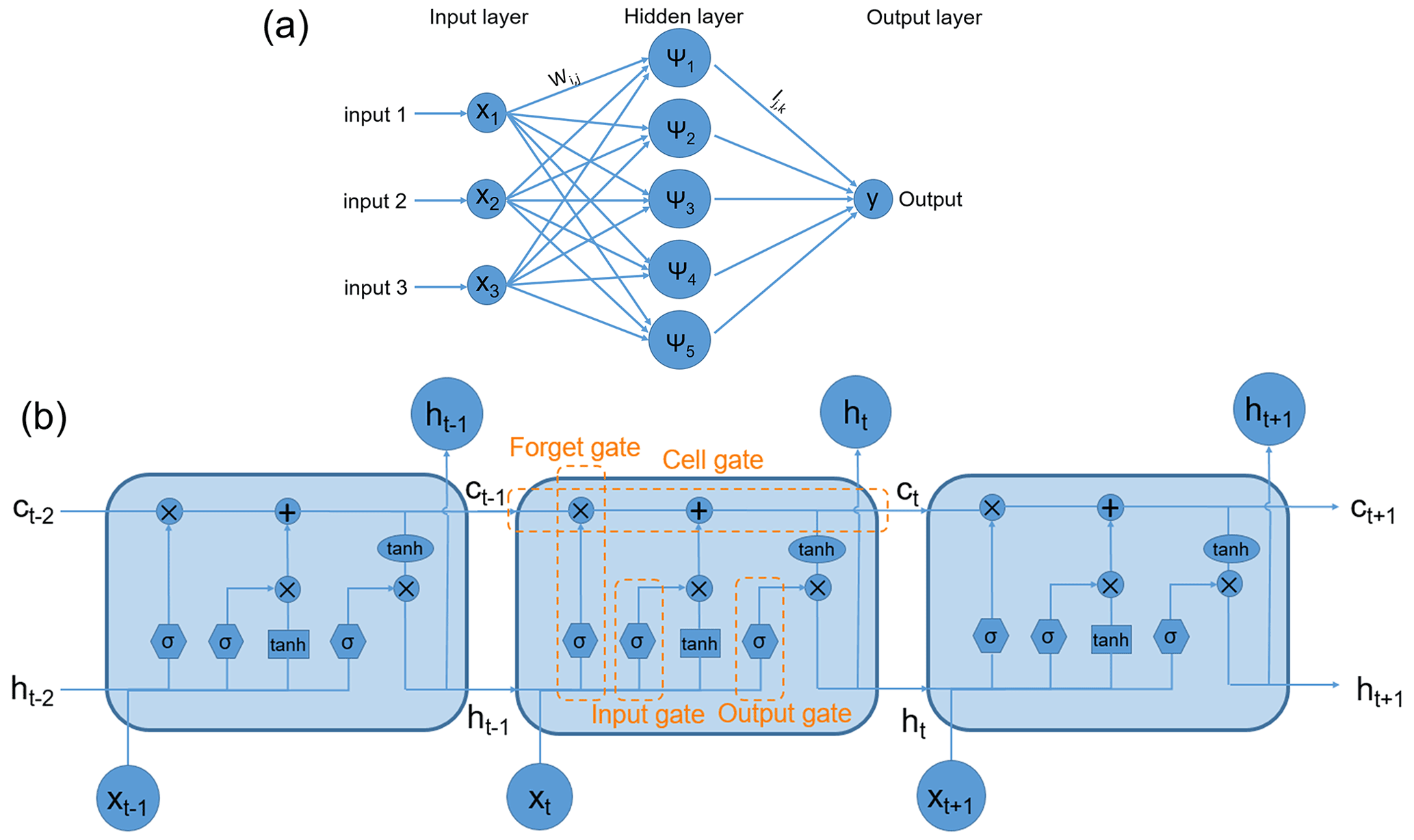
Figure 3Architecture of (a) a typical three-layer multi-layer perceptron (MLP) neural network and (b) a typical long-short time memory (LSTM) network. Ψi denotes the sigmoid transfer function, Wi,j represents connection weights between the input layer and the hidden layer, Ij,k represent connection weights between the hidden layer and the output layer. xt, ct, and ht represent the standardized input variable, hidden gate and cell gate at the current time t.
In this study, the variables included in the input layer are precipitation, temperature and SMS, whereas the variable included in the output layer is the detrended TWSA. Based on trial and error, the most optimal number of hidden neurons is set to five. After minimizing the discrepancy between the simulated TWSA with the observed results at the output layer, the most optimal network architecture can finally be obtained.
4.2 Long short-term memory network (LSTM)
The recurrent neural network (RNN) (Rumelhart et al., 1986) is a unique type of deep learning algorithm that was developed to process sequential data and predict future trends. One of the most dominant features of the RNN layer is a unique feedback connection which can allow past information to continuously affect the current output. The characteristics of all related time series data can be eventually learned through this structure. The long short-term memory network (LSTM) is one of the most representative RNNs as it has a fabulous memory ability and can effectively avoid the vanishing gradient problem existing in other RNNs (Hochreiter and Schmidhuber, 1997; Guo et al., 2021). Considering the time series characteristics of meteorological data and TWSA data, the LSTM model is very suitable as a statistical downscaling model for its excellent capacity to process sequence-to-sequence learning problems.
One typical LSTM model usually consists of three layers, that is, an input layer, a hidden layer and an output layer (Fig. 3b). Different from other traditional ANNs, the LSTM model replaces the hidden block in RNNs with a memory cell state coupled with three logic gates, that is, the forget gate, the input gate and the output gate. In the training process, the memory cell state mainly stores the accumulation of past information. The input gate determines how much information of a new input flows into the memory cell state at the current time. Then, the useless information in long-term memory would be forgotten by the forget gate, which determines how much of the former moment is retained to the current time. Finally, the output gate determines how much information of the memory cell state is used to compute output (Bai et al., 2021; Wu et al., 2020; Vu et al., 2021).
4.3 Multiple linear regression (MLR)
Multiple linear regression (MLR) is a typical statistical approach that can be applied to establish the relationships between inputs and outputs (Sousa et al., 2007). This approach has a wide range of hydrological applications since it can explain the linkage between various variables well (Lyu et al., 2021; Ramesh et al., 2020; Sun et al., 2020). Here we assume that the GRACE-/GRACE-FO-derived TWSA is linearly regressed onto the meteorological variables (i.e., precipitation and temperature) and the SMS obtained from GLDAS 2.1 simultaneously, that is
where y represents TWSA at monthly (or daily) scales; xi (i=3) represents three independent inputs including precipitation, temperature and SMS at monthly (or daily) scales; ai represents the corresponding regression coefficients of each input, which can be calculated by the least-squares regression method; and b represents a constant offset.
4.4 Flood event selection
A nonparametric algorithm suggested by Tarasova et al. (2018) is adopted to identify runoff events in this study, which has been widely applied in many different basins over the world because of its advantages in identifying flood events (Fischer et al., 2021; Giani et al., 2022; Lu et al., 2020; Winter et al., 2022). The brief procedure of this algorithm is described as follows: (1) picking out local minima within nonoverlapping 5 d windows with respect to the entire streamflow time series; (2) examining the extracted series of minima with the goal of finding turning points, all of which are usually defined as the points that are at least 1.11 times smaller than their neighboring minima; (3) reconstructing the base flow hydrograph according to the linear interpolation between the turning points, which are previously obtained in Step (2); and (4) screening the streamflow time series to identify runoff events after the separation of base flow. Traditionally, a typical runoff event can be characterized by three main components, namely peak, beginning and end points. A peak refers to the maximum of streamflow for a specific period. The beginning point refers to the closest point in time when total runoff is equal to base flow before the peak. Similarly, the end point denotes the closest point in time when total runoff is equal to base flow after the peak.
4.5 Daily flood potential index
The flood potential index provides a surrogate measure of the potential flood risks for a specific region, which can be obtained from monthly average precipitation anomalies and GRACE-derived TWSA (Reager and Famiglietti, 2009). In this study, we further propose a new normalized daily flood potential index (NDFPI) with reference to Reager and Famiglietti (2009) and Abhishek et al. (2021). Compared to the original flood potential index, the NDFPI can not only provide useful information on the early signs of the region's transition from a normal state to a flood-prone situation, but also effectively detect the flood events at sub-monthly timescales, which is calculated via the following steps:
where TWSAdef(t) (mm) represents the terrestrial water storage deficit for a specific day (t) that is defined as the difference between the historic storage anomaly time series maximum during the entire period (TWSAmax) and the storage amount from the previous day (TWSA (t−1)).
Then, the daily flood potential amount (DFPA) is further calculated as follows:
where DFPA (t) (mm) represents the daily flood potential amount for a specific day (t), P(t) (mm) represents the daily precipitation, and TWSA (t−1) (mm) represents the TWSA from the previous day (t−1).
Finally, we can calculate the normalized daily flood potential index (NDFPI) from the DFPA with the goal of removing the effects of hydrological heterogeneity varying from region to region and the typical difference between the storage change and precipitation that may not always result in floods (Reager and Famiglietti, 2009), which can be described as follows:
where DFPAmax and DFPAmin represent the maximum DFPA and minimum DFPA during the study period respectively. The NDFPI indicates the corresponding probability of flood occurrence with a range from 0 to 1. More flooding is likely to occur when the NDFPI is closer to 1 for a specific region.
4.6 Model test design
Monthly TWSA estimates during the extreme flood events occurred in the YRB can be reconstructed at regional scales based on the above three different learning-based models, namely the MLP model, the LSTM model and the MLR model. Meanwhile, these three models are further validated in four different basins covering the upstream to downstream parts of the Yangtze River in order to better evaluate their applications. For more detailed information about all these four different basins, the reader can also refer to Table S1 in the Supplement. According to previous findings in Liu et al. (2021), different periods of data used for training (i.e., identification of model parameter sets) and validation can eventually influence the corresponding performances of a specific model when simulating TWSA. Therefore, we design a total of three scenarios according to the way of dividing training periods and validation periods for a specific model. As shown in Fig. 2, periods of GRACE data used for training and validation in each experiment are listed, which include (1) Scenario 1, training period (January 2003–July 2014, a total of 129 months) and validation period (August 2014–December 2020, a total of 56 months); (2) Scenario 2, training period (June 2005–June 2018, a total of 129 months) and validation period (January 2003–May 2005 and July 2018–December 2020, a total of 56 months); and (3) Scenario 3: training period (October 2007–December 2020, a total of 129 months) and validation period (January 2003–September 2007, a total of 56 months).
Furthermore, three kinds of statistical measures including the root mean square error (RMSE), correlation coefficient (r), and Nash–Sutcliffe efficiency coefficient (NSE) are used in this study as they can jointly measure the matching quality in terms of both magnitude and phase between the simulated and the observed time series. These statistical measures are defined as
where xs,i and xo,i represent the simulated and observed TWSA in month i, respectively; and represent the average of simulated and observed TWSA series; and N is the total months of observed (or simulated) TWSA available.
5.1 Temporal variation of precipitation, temperature, SMSA, TWSA and streamflow across the YRB during 2003–2020
Figure 4 shows the monthly time series of SMSA, TWSA, streamflow and the main climatic variables including precipitation and temperature across the YRB during 2003–2020. The results show that monthly TWSA over the YRB has a wide range from −58.0 to 130.9 mm during the study period. Monthly TWSA estimated by three GRACE and GRACE-FO solutions changes synchronously with precipitation across the entire YRB, showing a significantly positive correlation between TWSA and precipitation (r=0.54; p<0.01) during the study period. According to the statistics collected by Yangtze River Conservancy Commission of Ministry of Water Resources, the accumulative rainfall across the entire YRB exceeds 680 mm in summer 2020 from April to October, which is far more than the mean rainfall (approximately 540 mm) during the same period from 2003 to 2019. Accordingly, TWSA reaches its maximum in July 2020 with an estimate of 130.9 mm during 2003–2020, reflecting the evolution of TWSA in response to heavy rainfall during this period. In addition to precipitation, TWSA is also highly consistent with temperature over the YRB during 2003–2020, showing a positive correlation coefficient of r=0.57 (p<0.01) with monthly temperature.
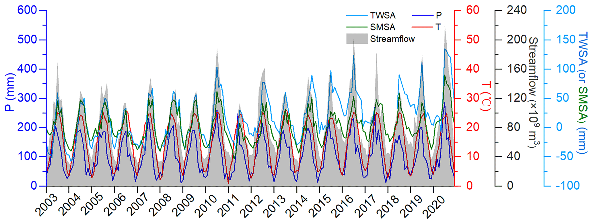
Figure 4Monthly time series of precipitation (P; mm), temperature (T; ∘C), terrestrial water storage anomaly (TWSA; mm), soil moisture storage anomaly (SMSA; mm) and streamflow (×109 m3) across the YRB during 2003–2020. Streamflow data are obtained at the Datong hydrological station (shown in Fig. 1). YRB: Yangtze River basin.
The GLDAS Noah-derived SMSA and GRACE-/GRACE-FO-derived TWSA both show a seasonal variation through the entire study period in the YRB, but there is a significant difference in the intensity of anomalies between them, especially in the summer season, as depicted in Fig. 4. This phenomenon can be explained by the discrepancies resulting from the components of SMSA and TWSA. Although the SMSA is an important component of the TWSA for many regions, the latter usually contains some other components, such as the anomalies of surface water and groundwater, besides the SMSA (Xie et al., 2021). There is a significant correlation between the TWSA and SMSA, with a positive correlation coefficient of r=0.84 (p<0.01), both of which reach maximum and minimum values almost simultaneously. In general, the TWSA shows a significant correlation with precipitation, temperature and the SMSA during the study period, all of which have been therefore selected as the inputs applied to simulate the monthly TWSA over different regions.
5.2 Reconstruction of TWSA by different models
To achieve the temporal downscaling of monthly TWSA data and fill the missing months for TWSA, we should firstly build the relationships between GRACE-/GRACE-FO-derived TWSA and various hydroclimatic factors including precipitation, temperature and the SMSA at monthly timescales. The results of the TWSA are estimated by the mean value in different regions upstream of the corresponding hydrological stations shown in Fig. 1. In this study, three different models including MLP, LSTM and MLR are adopted to reconstruct TWSA for regions. Table 3 shows the summary of model performances in reconstructing monthly TWSA across the YRB during the study period. GRACE and GRACE-FO satellite data used for training (i.e., identification of model parameter sets) and validation shown in each scenario mainly depend on the periods of series of data, as suggested by Liu et al. (2021). According to Table 3, we find that all models including the MLP, the LSTM and the MLR with Scenario 3 show the best performances in simulating monthly TWSA under all three designed scenarios. This result indicates that the models with Scenario 3 are relatively superior to the models with the other two scenarios when simulating TWSA because the data in Scenario 3 contain more extremely high (or low) values during the study period in the process of training models. Therefore, in the following sections, we decide to directly divide the training periods and validation periods of all these models according to Scenario 3 (shown in Table 3) when simulating the monthly TWSA for other regions besides the YRB.
Table 3Performances of different models in simulating monthly TWSA across the YRB during 2003–2020.
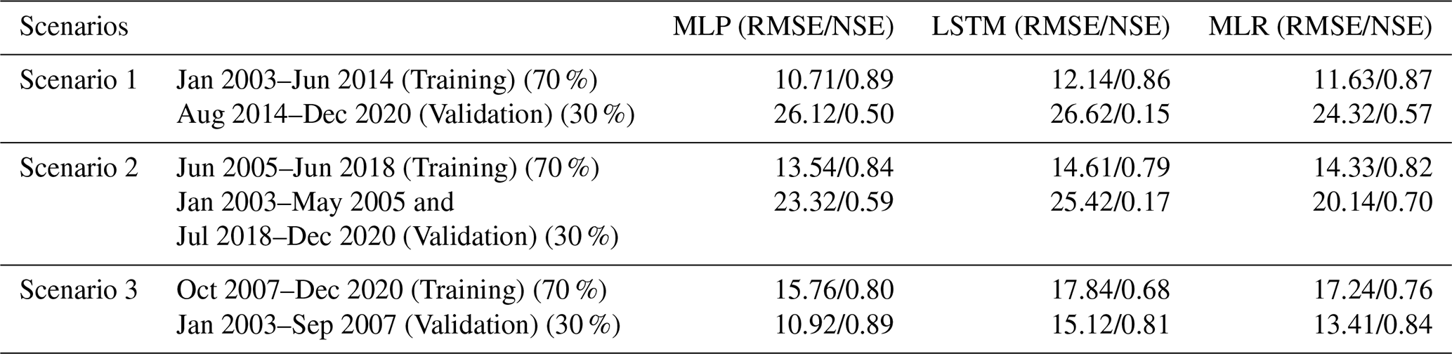
TWSA: terrestrial water storage anomalies. YRB: Yangtze River basin. MLP: multi-layer perceptron neural network. LSTM: long short-term memory network. MLR: multiple linear regression. 70 %, 30 % and 100 % represent the corresponding proportions to all samples in the training, the validation and the entire periods respectively. RMSE and NSE represent the root mean square error (mm per month) and Nash–Sutcliffe efficiency coefficient between the simulated TWSA with the observed TWSA respectively. Note that the GRACE-/GRACE-FO-derived TWSA in some months is not available due to the problem of battery management.
Figure 5 shows the comparison between the monthly TWSA derived from GRACE and GRACE-FO satellite data and that simulated by different models for all regions during 2003–2020. The corresponding evaluation values are also presented in this figure. We find that the maximum NSEs between the GRACE-/GRACE-FO-derived TWSA estimates and those simulated by models are 0.68, (Fig. 5a), 0.82 (Fig. 5f), 0.86 (Fig. 5g) and 0.89 (Fig. 5j) during the validation periods for the SYRB, the UYRB, the UMYRB and the YRB, respectively. The corresponding RMSEs are 13.2, 13.7, 12.4 and 10.9 mm per month (validation periods, hereafter) for the SYRB, the UYRB, the UMYRB and the YRB, respectively. In general, the detrended TWSA estimates present consistent values between the observations and the modeled results from 2003–2020 for most regions except for the SYRB, as shown in Fig. 5. Compared to the other regions, all models show a relatively poor performance in simulating monthly TWSA for the SYRB with NSEs less than 0.70 during the validation periods, which can be mainly attributed to the increased uncertainties in precipitation and temperature induced by the sparse distribution of meteorological stations over this region (shown in Fig. 1).
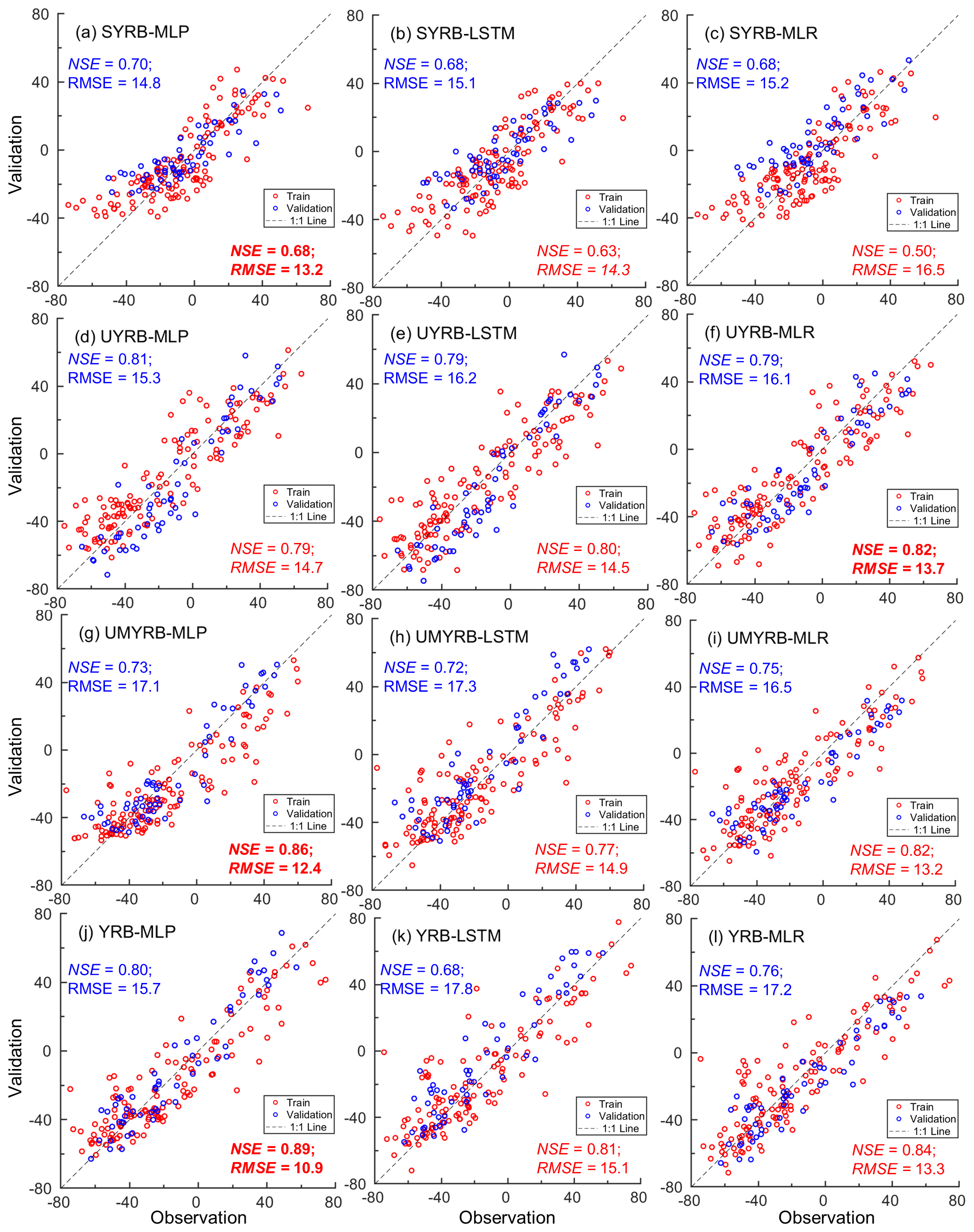
Figure 5Comparison between the monthly TWSA derived from GRCACE/GRACE-FO satellite data (observation) and that simulated by different models (validation) for (a–c) the SYRB, (d–f) the UYRB, (g–i) the UMYRB and (j–l) the YRB respectively during 2003–2020, showing statistics of the comparison including root mean square error (RMSE) (mm per month) and Nash–Sutcliffe efficiency (NSE). Note that TWSAs shown in this figure are detrended because hydroclimatic factors may not fully simulate all the long-term trends. The models showing the best performance in simulating the TWSA during the validation periods are bold for each region. SYRB: source regions of Yangtze River basin. UYRB: upper regions of Yangtze River basin. UMYRB: upper and middle regions of Yangtze River basin. YRB: Yangtze River basin.
We further separately compare the performances of all models in simulating monthly TWSA for a specific region. Taking the entire YRB as an example (Fig. 5j–l), GRACE-/GRACE-FO-derived TWSA estimates show a RMSE of 10.9 mm per month for the MLP-derived TWSA estimates, which is lower than that of 15.1 mm per month for the LSTM-derived TWSA estimates (∼ 39 % difference) and that of 13.3 mm per month for the MLR-derived TWSA estimates (∼ 22 % difference). Meanwhile, the NSE shows similar improvements when applying the MLP model to simulate the TWSA for the YRB (Fig. 5j–l), which can also be found in the SYRB (Fig. 5a–c) and the UMYRB (Fig. 5g–i). In general, the MLP and MLR models achieve high metrics (0.81/12.8 and 0.75/14.2 mm per month of NSE/RMSE on average for all regions) during the validation periods, both of which are significantly higher than the metrics between the GRACE-/GRACE-FO-derived TWSA estimates and that simulated by the LSTM model (0.75/14.7 mm of NSE/RMSE on average for all regions). For the UYRB (Fig. 5d–f), the MLP model shows a slightly poorer performance in simulating TWSA in terms of a higher RMSE (14.7 mm per month) than the LSTM model (14.5 mm per month; ∼ 1.2 % increase) and the MLR model (13.7 mm per month; ∼ 7.2 % increase). In addition, it seems that the larger the study region, the higher the correspondence between the GRACE-/GRACE-FO-derived TWSA estimates and that simulated by models for the MLP model. This result can be explained in that the large area for a specific region may smooth more uncertainties in GRACE signals and meteorological observations (Long et al., 2015).
Overall, Fig. 5 clearly suggests the MLP model's superior performances in simulating the TWSA, with an average value of NSE of 0.81 and an average value of RMSE of 12.8 mm per month during the validation periods for all regions, showing the outstanding capability of the MLP model in learning the complicated relationships between the TWSA and hydroclimatic factors. As documented in Shu and Ouarda (2007), the MLP model can show its unique superiority and great advantages compared with other statistical models, particularly when explaining the underlying processes that have complex nonlinear interrelationships. The results shown in Fig. 5 also indicate that the MLP model can show a relatively better performance in simulating monthly TWSA than the LSTM model in this study. As described in Zhang et al. (2018), one of main drawbacks of the LSTM model is its complexity compared with the MLP model, which indicates that the LSTM model may not show better performances in simulating time series data than other traditional ANN models in some cases, especially when limited trained data are available. In addition, the moderate performance of LSTM model in reconstructing TWSA compared to the MLP model can be partly attributed to the possibly limited role of the memory function in the LSTM model (Wei et al., 2021; Yin et al., 2022), since relations between inputs and the output of this model (shown in Fig. 4) are pretty direct without many memory effects. Therefore, in the following discussion, only the MLP model is applied to further achieve the temporal downscaling of monthly TWSA data for regions.
5.3 Temporal downscaling of GRACE and GRACE-FO satellite data
Relationships between monthly TWSA and hydroclimatic inputs with respect to the entire YRB have been fully established, as presented in Sect. 5.2. As documented in Herath et al. (2016) and Requena et al. (2021), the same scaling properties have been commonly assumed for baseline and future periods in temporal downscaling. Therefore, it is reasonable and acceptable to assume that scaling properties at monthly timescales are valid at daily timescales in this study (Kumar et al., 2012). That is, the relationship between temporally downscaled TWSA and daily hydroclimatic inputs is consistent with that previously established by the downscaling model (e.g., the MLP model) at monthly timescales for a specific region. By merging the daily hydroclimatic inputs into the previously established relationships between TWSA estimates and hydroclimatic factors based on the MLP model, we can downscale the TWSA estimates from monthly time series to daily time series for all regions.
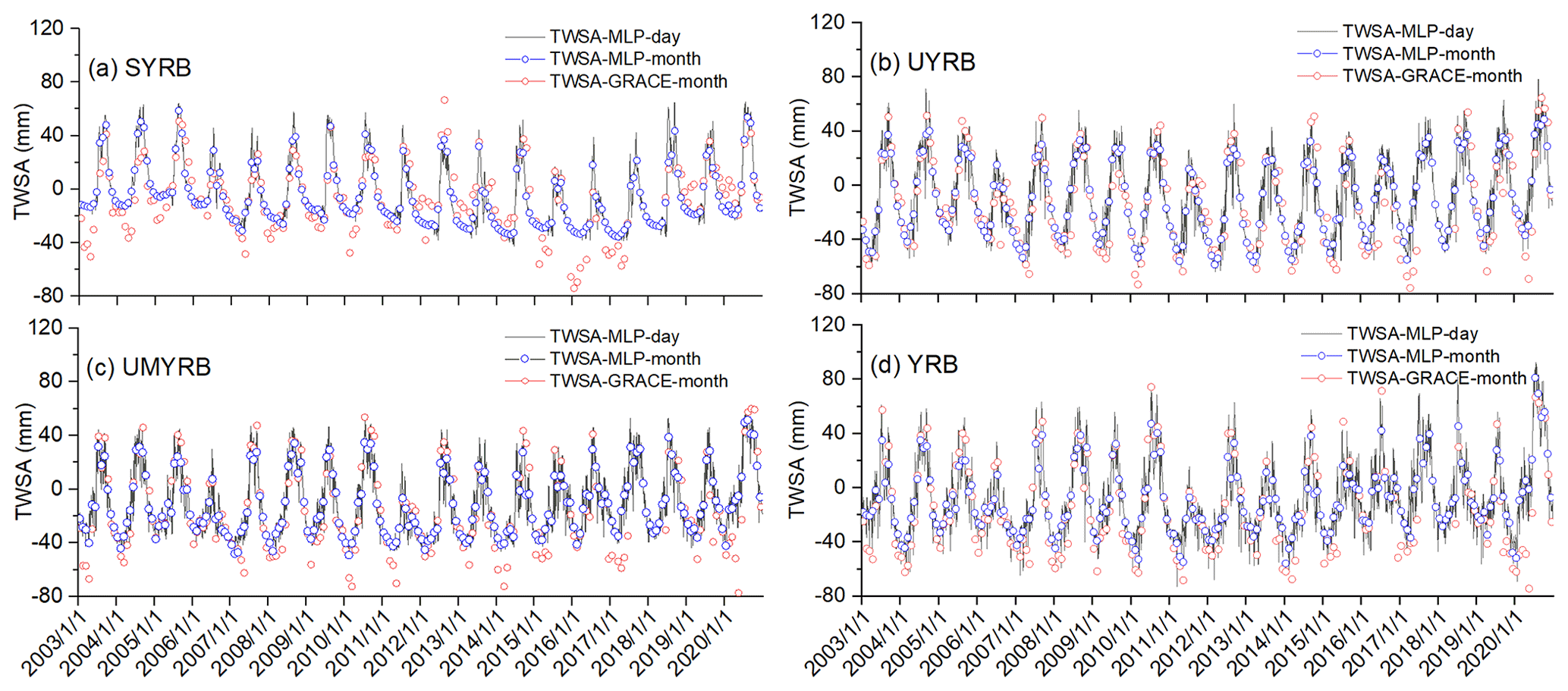
Figure 6Daily (TWSA-MLP-day) and monthly (TWSA-MLP-month) time series of the TWSA simulated by the MLP model for (a) the SYRB, (b) the UYRB, (c) the UMYRB and (d) the YRB respectively during 2003–2020. Note that monthly TWSA estimates derived from GRACE and GRACE-FO satellite data (TWSA-GRACE-month) shown in this figure are detrended because hydroclimatic factors may not fully simulate their long-term trends. TWSA: terrestrial water storage anomaly. MLP: multi-layer perceptron neural network. SYRB: source regions of Yangtze River basin. UYRB: upper regions of Yangtze River basin. UMYRB: upper and middle regions of Yangtze River basin. YRB: Yangtze River basin.
Figure 6 shows daily time series of the TWSA temporally downscaled by the MLP model for different regions during 2003–2020. It can be seen that the daily TWSA shows sub-monthly signals in response to changes in hydroclimatic factors as expected. Both GRACE-/GRACE-FO-derived TWSA estimates and daily TWSA estimates temporally downscaled by the MLP model show obvious seasonal cycles and reach their respective extreme values almost simultaneously. More specifically, amplitudes of daily TWSA estimates are slightly higher (or lower) than monthly TWSA estimates in summer (or winter) seasons from 2003 to 2020. This can be deemed reasonable because monthly TWSA estimates are defined as the mean average of daily TWSA estimates for a specific month. It should also be noted that there are still some discrepancies between temporally downscaled TWSA at sub-monthly timescales and monthly TWSA estimates derived from GRACE and GRACE-FO satellite data for the SYRB, particularly in some extreme low values, which can be attributed to the relatively poor relationship between TWSA estimates and hydroclimatic factors for this region, as described in Fig. 5a. As documented in previous studies (Liu et al., 2020; Shi et al., 2020), it has long been challenging to accurately perform hydrological simulations across the SYRB because of the complex hydrological processes in this alpine basin. For example, parameter settings calibrated by GLDAS Noah land surface model might not be highly accurate for SMS simulation across the SYRB because field measurements of SMS in this region are extremely limited. Harsh climatic conditions and limited weather stations can additionally influence the accuracy of meteorological observations such as precipitation and temperature across the SYRB, especially for some extreme values. Given the above reasons, there is a relatively poor relationship between TWSA estimates and hydroclimatic factors across the SYRB based on the MLP (shown in Fig. 5a). Furthermore, the uncertainties in the observed precipitation and temperature and SMS derived from the GLDAS Noah land surface model can eventually result in some discrepancies between the temporally downscaled TWSA at sub-monthly timescales and monthly TWSA estimates derived from GRACE and GRACE-FO satellite data, as described in Fig. 6a.
5.4 Relation between daily TWSA and streamflow during flood events
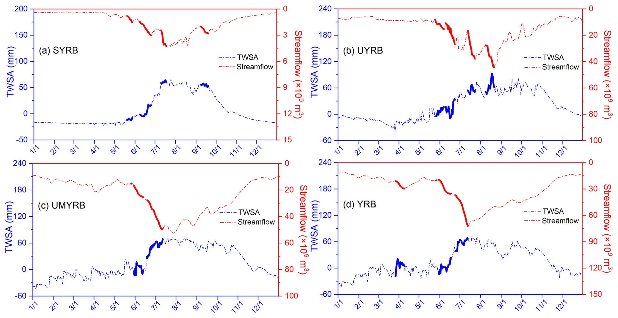
Figures 7 and 8 show the daily TWSA temporally downscaled by the MLP model and observed streamflow within the YRB in 2010 and 2020 when extreme flood events occurred according to the information published by the Yangtze River Conservancy Commission of Ministry of Water Resources. As described in Figs. 7 and 8, the nonparametric simple smoothing method introduced in Sect. 4.4 can effectively identify the corresponding flood events that occurred in each region based solely on the analysis of streamflow time series. It shows an apparent increase in streamflow from the beginning to the peak of all flood events. Accordingly, the daily TWSA shows a distinct increase similar to streamflow during the same periods as expected. It is also interesting to note that the beginning of the increase shown in the daily TWSA is earlier than that of streamflow. This is partly because high antecedent soil moisture, which is an important component of TWSA, has been identified as an important driver of flood events for regions (Fatolazadeh and Goïta, 2022; Jing et al., 2020; Reager et al., 2014; Wasko and Natthan, 2019). Meanwhile, this result indicates that the daily TWSA can be potentially useful in building early flood warning systems since it may identify the extreme flood events much more earlier than streamflow.
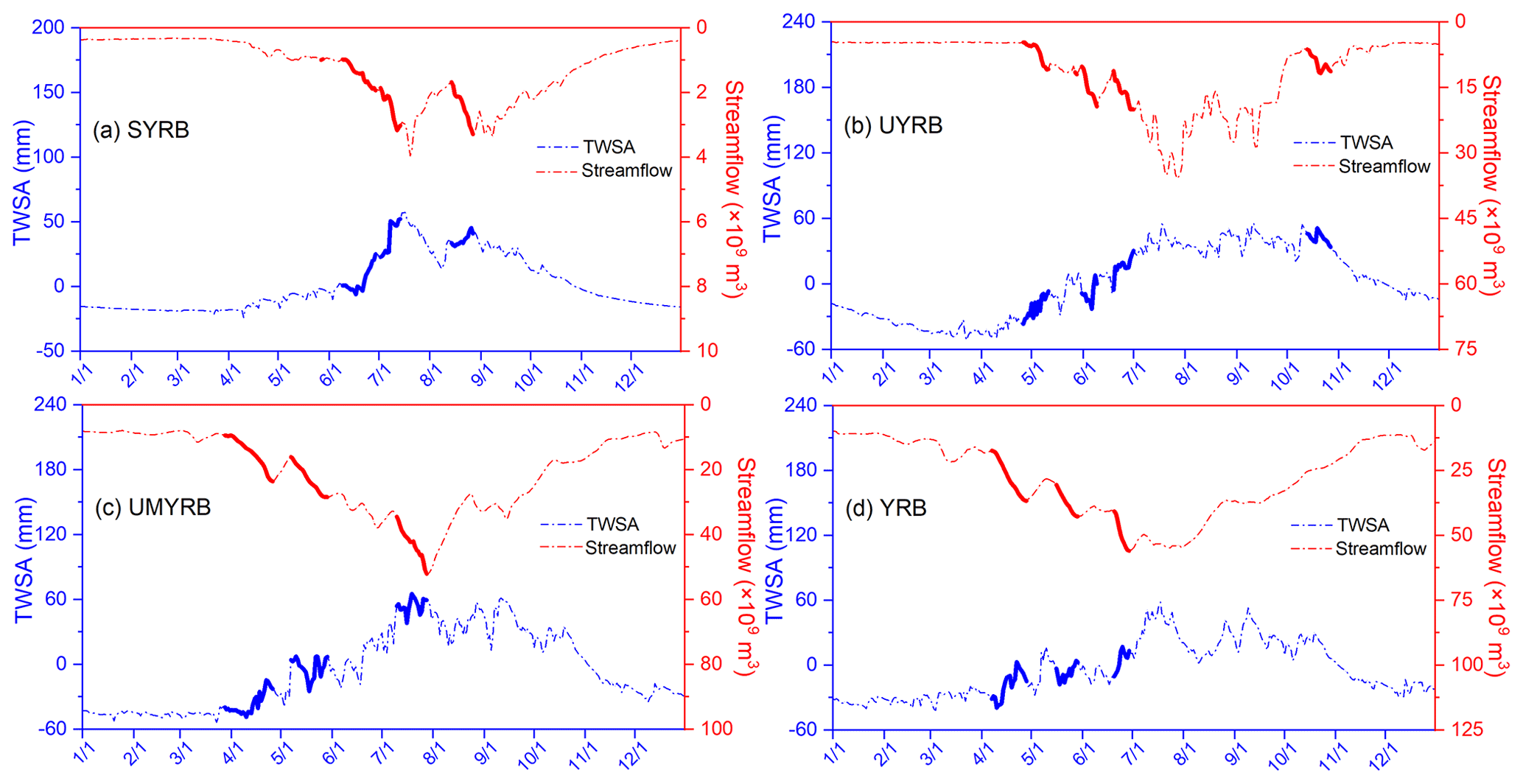
Figure 7Daily TWSA temporally downscaled by the MLP model versus streamflow during flood events across (a) the SYRB, (b) the UYRB, (c) the UMYRB and (d) the YRB respectively in 2010. The bold dashed blue lines and bold dashed red lines represent daily TWSA and streamflow during the period between the beginning and end of each runoff event. TWSA: terrestrial water storage anomaly. MLP: multi-layer perceptron neural network. SYRB: source regions of Yangtze River basin. UYRB: upper regions of Yangtze River basin. UMYRB: upper and middle regions of Yangtze River basin. YRB: Yangtze River basin.
5.5 Monitoring severe flood events based on the proposed NDFPI in the year 2020
To better monitor severe flood events over the YRB, we propose a new index, i.e., NDFPI, by jointly using the temporally downscaled TWSA data and daily precipitation data, as introduced in Sect. 4.5. According to the Yangtze River Conservancy Commission of Ministry of Water Resources, the YRB suffered from catastrophic flooding in the year 2020. Therefore, in this study, the severe flood events that occurred in 2020 for the YRB will serve as an example to present the capability of NDFPI in detecting extreme flood events. The threshold values of daily streamflow and NDFPI for the 90th percentile floods during 2003–2020 are presented in Fig. 9. According to the results shown in Fig. 9, the larger threshold values of NDFPI usually indicate severity of flood occurrence increases for a specific region. In addition, the shape of percentile duration curve of daily streamflow across the UYRB (Fig. 9b) is different to that shown in other regions. It is noted that the outlet of the UYRB, the Yichang hydrological station, is located approximately 45 km downstream of the Three Gorges Reservoir (shown in Fig. 1), which is one of the largest hydroelectric reservoirs in the world. Given that the operations of the Three Gorges Reservoir can directly affect the streamflow at Yichang station (Yang et al., 2022), the result shown in Fig. 9b is reasonable.
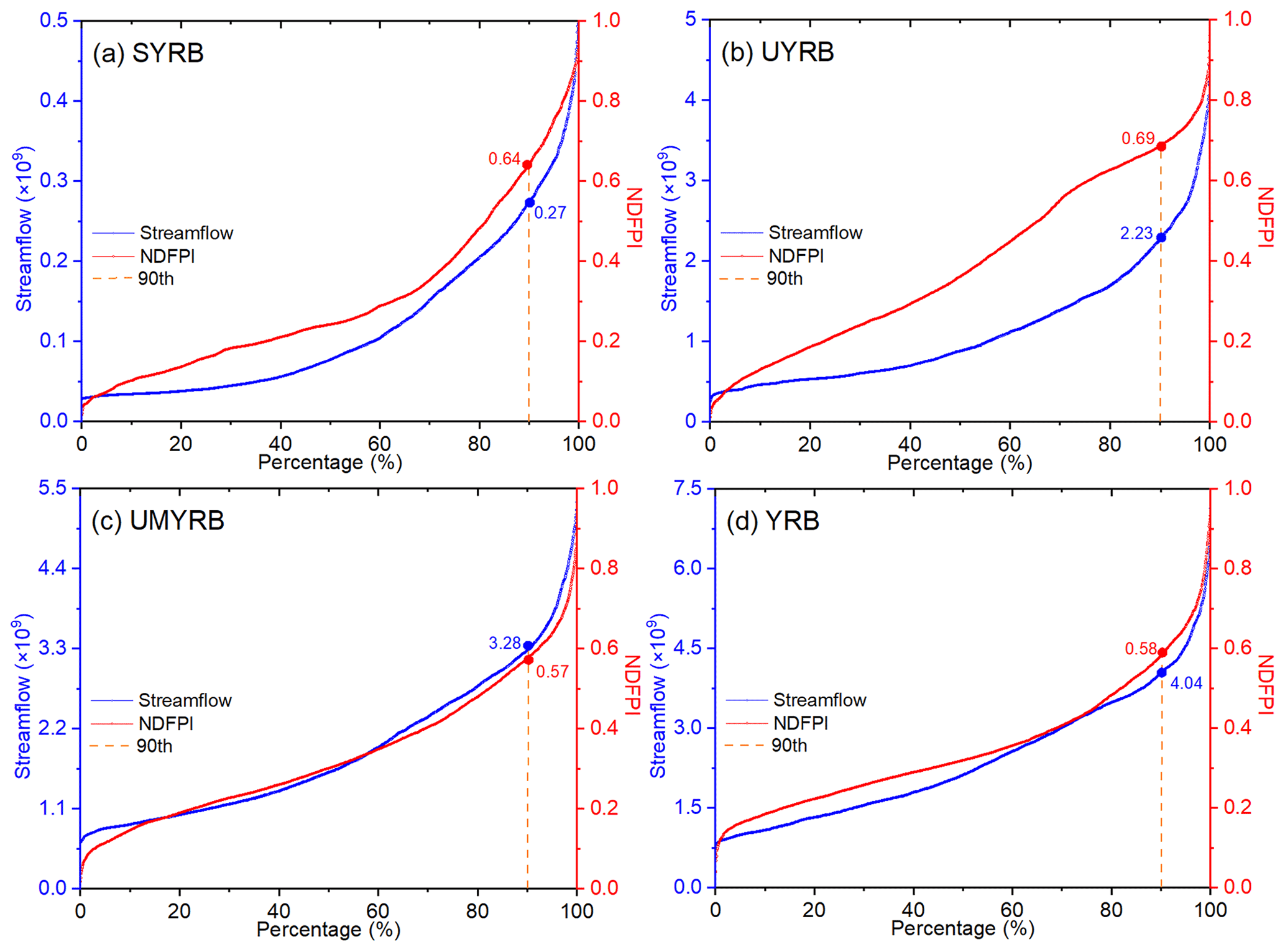
Figure 9Percentile duration curves of daily streamflow observations and NDFPI for the 90th percentile floods across (a) the SYRB, (b) the UYRB, (c) the UMYRB and (d) the YRB respectively during 2003–2020. The red dots and blue dots represent threshold values of daily streamflow and NDFPI for the 90th percentile floods across different regions. SYRB: source regions of Yangtze River basin. UYRB: upper regions of Yangtze River basin. UMYRB: upper and middle regions of Yangtze River basin. YRB: Yangtze River basin. NDFPI: normalized daily flood potential index.
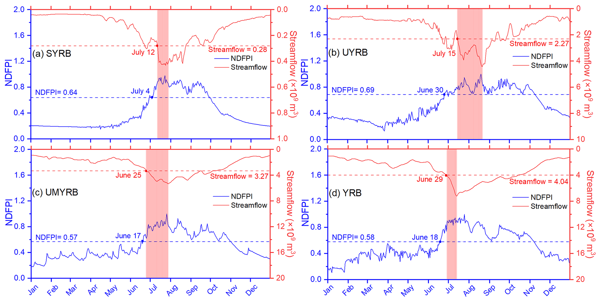
Figure 10Comparison between basin-averaged NDFPI and daily streamflow observations for the 90th percentile floods in 2020 across (a) the SYRB (observed at Shigu station), (b) the UYRB (observed at Yichang station), (c) the UMYRB (observed at Hankou station) and (d) the YRB (observed at Datong station). Pink rectangles denote the duration period between the thresholds of daily streamflow for the 90th percentile floods and peak streamflow observed at the controlling hydrological stations over different regions. The thresholds of daily streamflow and NDFPI for the 90th percentile floods are represented by the dashed red lines and dashed blue lines respectively. Note that the scales of streamflow shown in each figure are not always the same. SYRB: source regions of Yangtze River basin. UYRB: upper regions of Yangtze River basin. UMYRB: upper and middle regions of Yangtze River basin. YRB: Yangtze River basin. NDFPI: normalized daily flood potential index.
Figure 10 shows the comparison between basin-averaged NDFPI and daily streamflow observations for the 90th percentile floods in 2020. The results indicate that the ups and downs of the streamflow observed at different hydrological stations are highly consistent with the NDFPI results through the whole season. For example, the observations of streamflow from the Shigu hydrological station (Fig. 10a) reached the corresponding 90th percentile in 12 July. In comparison, the NDFPI estimated by the temporally downscaled TWSA and daily precipitation reached its 90th percentile in 4 July (Fig. 10a), which is 9 d earlier than that of daily streamflow. As expected, these high-streamflow observations during the wet season are usually accompanied by high NDFPI values, which could be attributed to the effects of high precipitation on streamflow during this period. For the YRB (Fig. 10d), daily streamflow detected at the Datong hydrological station reached its 90th percentile in 29 June and eventually peaked in 13 July, with a maximum value of 7.2×10⁹ m3 d−1, which is in line with the findings in Jia et al. (2021). Accordingly, the series of NDFPI reached its 90th percentile in 18 June with a value of 0.58. In general, Fig. 10 clearly suggests that the proposed NDFPI calculated by temporally downscaled TWSA data and daily precipitation changes synchronously with the reality of flood disasters in 2020 for the YRB. Meanwhile, it also indicates that such flood events can be monitored by the proposed NDFPI earlier than traditional streamflow observations.
Previous studies usually focus on monitoring the long-term flood events, while the flood events at sub-monthly timescales using GRACE and GRACE-FO satellite data have been limitedly investigated due to the limitation of their temporal resolution (i.e., month) (Gouweleeuw et al., 2018; Long et al., 2014). In this study, however, Fig. 10 clearly shows the incremental process of TWSA during the wet season using the newly proposed NDFPI estimated by temporally downscaled GRACE and GRACE-FO satellite data and daily precipitation for different regions. This means that the proposed NDFPI has the great potential to detect the evolution of extreme flood events within the short period. It is also interesting to note that the NDFPI reached the threshold of different classes of flood events earlier than that defined by streamflow observations during the wet season in 2020, which can be repeatedly found in the SYRB, the UYRB, the UMYRB and the YRB (Fig. 10) respectively. The comparison results indicate that the lag time between the threshold values of flood events monitored by the NDFPI and that monitored by daily streamflow during the wet season ranges from 8 to 15 d for the 90th percentile floods among all regions in 2020, all of which are far less than the temporal resolution of original GRACE and GRACE-FO satellite data (i.e., month). In addition to the 90th percentile floods, we also compare the basin-averaged NDFPI and daily streamflow observations for the 95th and 99th percentile floods in 2020 (shown in Figs. S1–S4). The results also show that the series of NDFPI reached the threshold values earlier than that of daily streamflow observations for the 95th and 99th percentile floods. For example, there is a 11 d lag time between the threshold value of NDFPI and that of the streamflow observed by Datong hydrological station for the 99th percentile floods in 2020 (Fig. S4d), which provides useful information for accurate and timely flood forecasts and can be very beneficial for protecting people and infrastructure over regions in a changing climate.
6.1 Extreme flood events monitored by NDFPI
The comparison results indicate that the proposed NDFPI reached the threshold values of different classes of flood events earlier than that defined by streamflow observations in 2020 with respect to the YRB and its individual subbasins (shown in Figs. 8 and S1–S4). This is consistent with the results found at the Missouri River basin by Reager et al. (2014). Reager et al. (2014) indicated that the regional TWSA may lead river discharge slightly before the flood season, which can provide useful information on the signal of high streamflow in the coming flood season. However, the study of Reager et al. (2014) only demonstrated the application of GRACE data to characterize regional flood potential at monthly timescales. More accurate information about the complete hydrologic state of a specific region at sub-monthly timescales during the wet season has been limitedly investigated, which is very vital for flood warnings. Given this, we proposed a new index, i.e., NDFPI, by jointly using the temporally downscaled TWSA data and daily precipitation data to better analyze the hydrologic state of the study region during the wet season at finer timescales.
The comparison analysis of the NDFPI and daily streamflow with respect to the YRB may explain the possible reasons why the NDFPI can detect extreme flood events for a specific river basin. Intense rainfall of long duration can cause continuous increases in the surface water (e.g., water stored in lakes and wetlands), soil moisture storage and groundwater storage that are totally represented by the TWSA in this study through the process of infiltration. Many studies also revealed that changes in surface water, soil moisture and groundwater under intense rainfall can exert obvious effects on the status of regional TWSA (Döll et al., 2012; Felfelani et al., 2017; Sinha et al., 2019; Velicogna et al., 2012). All these changes may ultimately result in the saturation of aquifer over regions. However, the saturated state of aquifers is not persistent because there is a great need for the basin to relieve its saturated state by discharging excessive water stored on and below the land surface into the river channels, which may eventually lead to the dramatic increase in streamflow and greatly increase the risk of widespread and damaging regional flooding.
6.2 Advantages of detecting extreme flood events based on temporally downscaled TWSA
The traditional flood monitoring approaches can provide useful information about the evolution of flood events over the study region through the measurements of rainfall and streamflow. All these measurements largely depend on the in situ hydrological stations and rainfall gauging stations distributed over the regions, which are difficult to achieve in some regions with harsh environment and climatic conditions. In comparison, satellite remote sensing has no such limitation of traditional point-based observations, making it a promising approach to monitor extreme flood events particularly in some poorly gauged basins. Given the large spatial extent, complicated climatic conditions and inaccessible hydrological observations for some high-altitude regions (e.g., SYRB), the GRACE TWSA has shown great advantages and superiority in flood monitoring and water resources management for the YRB than traditional flood monitoring approaches.
Furthermore, all these traditional flood monitoring approaches mainly focus on the meteorological conditions or the status of surface water reflected by various hydroclimatic factors and pay little attention to the importance of antecedent terrestrial water storage conditions before flood events, which can play a critical role in capturing the flood formation processes (Xiong et al., 2021b). For example, Reager and Famiglietti (2009) applied the TWSA from GRACE data and monthly precipitation to assess the likelihood for flooding at the regional scale and emphasized the importance of terrestrial water storage signal in the accurate prediction of floods and general runoff. Long et al. (2014) employed the index of flood potential amount using GRACE data and monthly precipitation to investigate hydrological floods and droughts for a large karst plateau in Southwest China and found that higher TWSA estimates are more prone to result in large potential for flooding during rainy season because of the excessive water that cannot be stored further. Therefore, the new proposed index incorporating the TWSA can more holistically quantify the potential of the development of severe floods for regions than common flood potential indices using hydroclimatic observations.
While previous studies have proposed several standardized indices for large-scale flood monitoring based on the GRACE-derived TWSA (Chen et al., 2010; Tangdamrongsub et al., 2016), flood monitoring and assessment at sub-monthly timescales remains a challenge using GRACE data due to its coarse temporal resolution (month). Flood monitoring at finer timescales is pivotal in understanding the regional water cycle under climate change, which ultimately helps to manage the basin-scale water resources effectively and improve the efficiency of early flood warning systems. The application of daily series of TWSA temporally downscaled from GRACE and GRACE-FO satellite data can provide a useful method to comprehensively assess the integrated flood conditions, considering the changes of both surface and subsurface water storage at sub-monthly timescales. The highest difference in the temporally downscaled TWSA and the daily precipitation during the wet season, as revealed by the NDFPI, can indicate the early signs of the region's transition from normal state to a flood-prone situation. Overall, the new proposed NDFPI is proven to be a useful tool for flood monitoring with the finer timescale over large-scale basins, which also makes it possible to monitor extreme flood events in a timely manner, especially for some regions with limited in situ streamflow observations.
6.3 Uncertainties and limitations
Using the method of linear detrending, long-term trends in series of TWSA estimates have been removed during the reconstruction of the TWSA because they are generally driven by various human activities such as irrigation, reservoir operation and water withdrawals, all of which cannot be well reconstructed by hydroclimatic factors (Humphrey and Gudmundsson, 2019). Although the detrending method can reduce the impacts of human activities on reconstructing the TWSA to some degree, it could still result in some discrepancies between the results of the detrended TWSA and the natural TWSA under climatic variability, particularly in some regions where intense human activities existed. In future, more attention should be paid to reconstruct the series of the regional TWSA under climatic variability when more detailed statistics related to human use such as water consumption, reservoir operation and inter-basin water diversion projects are available. Meanwhile, TWSA estimates in some months are not available for the GRACE and GRACE-FO satellite due to the problem of battery management. Although all these missing months can be effectively filled by different machine-learning-based models, this method may overestimate or underestimate the actual TWSA, especially for some extreme values in the peak of the wet or dry season (Abhishek et al., 2022).
Furthermore, this study presents an effective way to temporally downscale the TWSA estimates from monthly time series into daily values. This temporal downscaling method is assessed through four case studies across the entire YRB, which could present the temporal evolution of TWSA at sub-monthly timescales during the wet season well. As this study mainly focuses on characterizing regional flood potential based on the new proposed NDFPI incorporating temporally downscaled TWSA estimates, we applied this temporal downscaling method on the basin scale. In theory, this method is also suitable for the temporal downscaling of GRACE and GRACE-FO satellite data at the grid cell scale. However, as pointed out by previous studies (Landerer and Swenson, 2012; Save et al., 2016; Scanlon et al., 2016), gridded TWSA estimates derived from GRACE and GRACE-FO satellite data involved relatively large uncertainty induced by associated measurement errors and signal leakage errors. As a result, the accuracy of TWSA estimates can ultimately exert a direct influence on the optimized parameter sets that are obtained for trained models in each grid cell, which is a contributing factor of the uncertainty. In addition, the forcing data of these models used for temporal downscaling, including air temperature, precipitation and the GLDAS Noah-derived SMSA, may also contain some errors and uncertainties due to the uneven spatial distribution of meteorological stations and natural measurement errors (Lv et al., 2017). These errors and uncertainties from the input data could be propagated into the machine-learning-based models (e.g., MLP model), resulting in a broad range of differences between the observations and the simulated results. The latest study has made some initial attempts to learn the spatiotemporal patterns of difference between the TWSA derived from GRACE data and that simulated by land surface models based on the convolutional neural network (CNN) models, with the goal of providing more accurate TWSA estimates (Mo et al., 2022; Sun et al., 2019). Therefore, thorough consideration of the spatiotemporal patterns of difference between the TWSA derived from GRACE and GRACE-FO satellite data and that simulated by other hydrological models will be further taken in our future work when downscaling the TWSA estimates in order to better understand the complex underlying mechanism for TWSA variations during the wet season. Additionally, more efforts should be made to further validate the reliability of temporally downscaled relations proposed in this study when more independent data sources (e.g., groundwater level measurements) are available in YRB.
Overall, the present study shows the great potential of temporally downscaled GRACE and GRACE-FO satellite data in monitoring the extreme flood events. The study provides an effective means for the temporal downscaling of original TWSA estimates from GRACE and GRACE-FO satellite data and will help facilitate the sustainable management of water resources and develop monitoring and early-warning systems for severe flood events over large-scale basins. The methods and results shown in this study can provide important implications of flood hazard prevention and water resource management for other similar basins that are prone to suffer from severe extreme floods. Furthermore, this study can also provide broader implications for flood monitoring in ungauged or poorly gauged basins. For example, advances in satellite remote sensing have made remote sensing a promising approach to capture various hydrological variables (e.g., precipitation, temperature and soil moisture) (Table S2), since they can substantially reduce the limitations of traditional ground-based observations. This is extremely useful and important in hydrological research and applications, particularly in ungauged or poorly gauged basins. Therefore, we can calculate the flood potential index proposed in this study (i.e., NDFPI) by jointly using remote-sensing-based precipitation, temperature and soil moisture estimates combined with GRACE and GRACE-FO satellite data, which can further provide the potential of remote sensing data for flooding in ungauged or poorly gauged basins.
In the present study, we downscaled the GRACE-/GRACE-FO-derived TWSA estimates from monthly time series to daily time series in the YRB by establishing a relationship between TWSA estimates and hydroclimatic factors based on machine learning techniques. Furthermore, the temporally downscaled TWSA data combined with daily precipitation were adopted to monitor the extreme flood events over the entire YRB in 2020 based on a new daily flood potential index. The main conclusions can be drawn as follows:
-
When reconstructing the monthly TWSA in the YRB, the MLP model shows the best performance, with RMSE = 10.9 mm per month and NSE = 0.89. The MLR model follows with RMSE = 13.4 mm per month and NSE = 0.84, and the LSTM model shows the lowest performance, with RMSE = 15.1 mm per month and NSE = 0.81 during the validation period.
-
Based on the MLP model, monthly time series of TWSA were temporally downscaled to daily estimates using meteorological observations and the outputs from a land surface model. The results show high consistency with original monthly TWSA estimates derived from GRACE and GRACE-FO satellite data with regard to seasonal cycles.
-
By jointly using daily average precipitation anomalies and temporally downscaled TWSA, the proposed NDFPI can effectively detect the flood events that occurred in 2020 at sub-monthly timescales for the entire YRB.
-
The comparison analysis indicates that different types of flood events including the 90th, 95th and 99th percentile floods can be monitored by the proposed NDFPI earlier than traditional streamflow observations with respect to the YRB and its individual subbasins, which is very vital for flood forecasts and warning across this region.
The authors would like to thank both the China Meteorological Administration and the Yangtze River Conservancy Commission of Ministry of Water Resources (http://www.cjw.gov.cn/, last access: 17 November 2022) for providing the meteorological observations and hydrological data used in this study. The meteorological observations and hydrological data used in this study are available from the corresponding author upon request. We sincerely thank the NASA MEaSUREs Program and the Center for Space Research for providing GRACE/GRACE Follow-On JPL and CSR Level 3 Release 6 data, both of which are available from https://podaac.jpl.nasa.gov/GRACE?tab=mission-objectives§ions=about+data (NASA, 2022) and https://www2.csr.utexas.edu/grace/RL06_mascons.html (GRACE, 2022). We also sincerely thank the Goddard Earth Sciences (GES) Data and Information Services Center (DISC) for providing soil moisture storage acquired from the Global Land Data Assimilation System (GLDAS) data (https://doi.org/10.5067/E7TYRXPJKWOQ, Beaudoing and Rodell, 2020).
The supplement related to this article is available online at: https://doi.org/10.5194/hess-26-5933-2022-supplement.
YPX and JX designed the study. YPX guided the research and revised the manuscript. JX did the main calculations and wrote the draft of the manuscript. HY and YH performed data preprocessing. YG helped to process the raw GRACE data.
At least one of the (co-)authors is a member of the editorial board of Hydrology and Earth System Sciences. The peer-review process was guided by an independent editor, and the authors also have no other competing interests to declare.
Publisher's note: Copernicus Publications remains neutral with regard to jurisdictional claims in published maps and institutional affiliations.
We would like to thank our handling editor and the three anonymous referees, who provided valuable suggestions and input that substantially improved this paper.
This study is financially sponsored by the National Natural Science Foundation of China (grant nos. 52109037 and 52009121), the Zhejiang Key Research and Development Program (grant no. 2021C03017) and the Fundamental Research Funds for the Zhejiang Provincial Universities (grant no. 2021XZZX015).
This paper was edited by Fuqiang Tian and reviewed by three anonymous referees.
Abhishek, Kinouchi, T., and Sayama, T.: A comprehensive assessment of water storage dynamics and hydroclimatic extremes in the Chao Phraya River Basin during 2002–2020, J. Hydrol., 603, 126868, https://doi.org/10.1016/j.jhydrol.2021.126868, 2021.
Abhishek, Kinouchi, T., Abolafia-Rosenzweig, R., and Ito, M.: Water Budget Closure in the Upper Chao Phraya River Basin, Thailand Using Multisource Data, Remote Sens., 14, 173, https://doi.org/10.3390/rs14010173, 2022.
Ahmed, M., Aqnouy, M., and Messari, J. S. E.: Sustainability of Morocco's groundwater resources in response to natural and anthropogenic forces, J. Hydrol., 603, 126866, https://doi.org/10.1016/j.jhydrol.2021.126866, 2021.
Bai, P., Liu, X., and Xie, J.: Simulating runoff under changing climatic conditions: A comparison of the long short-term memory network with two conceptual hydrologic models, J. Hydrol., 592, 125779, https://doi.org/10.1016/j.jhydrol.2020.125779, 2021.
Beaudoing, H. and Rodell, M.: NASA/GSFC/HSL, GLDAS Noah Land Surface Model L4 3 hourly 0.25 × 0.25 degree V2.1, Greenbelt, Maryland, USA, Goddard Earth Sciences Data and Information Services Center (GES DISC) [data set], https://doi.org/10.5067/E7TYRXPJKWOQ, 2020.
Bomers, A., van der Meulen, B., Schielen, R. M. J., and Hulscher, S. J. M. H.: Historic flood reconstruction with the use of an Artificial Neural Network, Water Resour. Res., 55, 9673–9688, https://doi.org/10.1029/2019WR025656, 2019.
Boucher, M. A., Quilty, J., and Adamowski, J.: Data assimilation for streamflow forecasting using extreme learning machines and multilayer perceptrons, Water Resour. Res., 56, e2019WR026226, https://doi.org/10.1029/2019WR026226, 2020.
Chao, N., Jin, T., Cai, Z., Chen, G., Liu, X., Wang, Z., and Yeh, P. J. F.: Estimation of component contributions to total terrestrial water storage change in the Yangtze river basin, J. Hydrol., 595, 125661, https://doi.org/10.1016/j.jhydrol.2020.125661, 2021.
Chen, J. L., Wilson, C. R., and Tapley, B. D.: The 2009 exceptional Amazon flood and interannual terrestrial water storage change observed by GRACE, Water Resour. Res., 46, W12526, https://doi.org/10.1029/2010WR009383, 2010.
Chen, X., Jiang, J., and Li, H.: Drought and flood monitoring of the Liao River Basin in northeast China using extended GRACE Data, Remote Sens., 10, 1168, https://doi.org/10.3390/rs10081168, 2018.
Dottori, F., Szewczyk, W., Ciscar, J., Zhao, F., Alfieri, L., Hirabayashi, Y., Bianchi, A., Mongelli, I., Frieler, K., Betts, R. A., and Feyen, L.: Increased human and economic losses from river flooding with anthropogenic warming, Nat. Clim. Change, 8, 781–786, https://doi.org/10.1038/s41558-018-0257-z, 2018.
Döll, P., Hoffmann-Dobrev, H., Portmann, F. T., Siebert, S., Eicker, A., Rodell, M., Strassberg, G., and Scanlon, B. R.: Impact of water withdrawals from groundwater and surface water on continental water storage variations, J. Geodyn., 59–60, 143–156, https://doi.org/10.1016/j.jog.2011.05.001, 2012.
Fang, H., Han, D., He, G., and Chen, M.: Flood management selections for the Yangtze River midstream after the Three Gorges Project operation, J. Hydrol., 432-433, 1–11, https://doi.org/10.1016/j.jhydrol.2012.01.042, 2012.
Fatolazadeh, F. and Goïta, K.: Reconstructing groundwater storage variations from GRACE observations using a new Gaussian-Han-Fan (GHF) smoothing approach, J. Hydrol., 604, 127234, https://doi.org/10.1016/j.jhydrol.2021.127234, 2022.
Felfelani, F., Wada, Y., Longuevergne, L., and Pokhrel, Y. N.: Natural and human-induced terrestrial water storage change: A global analysis using hydrological models and GRACE, J. Hydrol., 553, 105–118, https://doi.org/10.1016/j.jhydrol.2017.07.048, 2017.
Fischer, S., Schumann, A., and Bühler, P.: A statistics-based automated flood event separation, J. Hydrol. X, 10, 100070, https://doi.org/10.1016/j.hydroa.2020.100070, 2021.
Giani, G., Tarasova, L., Woods, R. A., and Rico-Ramirez, M. A.: An objective time-series-analysis method for rainfall-runoff event identification, Water Resour. Res., 58, e2021WR031283, https://doi.org/10.1029/2021WR031283, 2022.
Gouweleeuw, B. T., Kvas, A., Gruber, C., Gain, A. K., Mayer-Gürr, T., Flechtner, F., and Güntner, A.: Daily GRACE gravity field solutions track major flood events in the Ganges–Brahmaputra Delta, Hydrol. Earth Syst. Sci., 22, 2867–2880, https://doi.org/10.5194/hess-22-2867-2018, 2018.
GRACE: CSR GRACE/GRACE-FO RL06 Mascon Solutions (version 02), GRACE [data set], https://www2.csr.utexas.edu/grace/RL06_mascons.html, last access: 17 November 2022.
Guo, Y., Yu, X., Xu, Y.-P., Chen, H., Gu, H., and Xie, J.: AI-based techniques for multi-step streamflow forecasts: application for multi-objective reservoir operation optimization and performance assessment, Hydrol. Earth Syst. Sci., 25, 5951–5979, https://doi.org/10.5194/hess-25-5951-2021, 2021.
Herath, S. M., Sarukkalige, P. R., and Nguyen, V. T. V.: A spatial temporal downscaling approach to development of IDF relations for Perth airport region in the context of climate change, Hydrolog. Sci. J., 61, 2061–2070, https://doi.org/10.1080/02626667.2015.1083103, 2016.
Hochreiter, S. and Schmidhuber, J.: Long short-term memory, Neural Comput., 9, 1735–1780, https://doi.org/10.1162/neco.1997.9.8.1735, 1997.
Huang, S., Zhang, X., Chen, N., Li, B., Ma, H., Xu, L., Li, R., and Niyogi, D.: Drought propagation modification after the construction of the Three Gorges Dam in the Yangtze River Basin, J. Hydrol., 603, 127138, https://doi.org/10.1016/j.jhydrol.2021.127138, 2021.
Huang, Y., Salama, M. S., Krol, M. S., Su, Z., Hoekstra, A. Y., Zeng, Y., and Zhou, Y.: Estimation of human-induced changes in terrestrial water storage through integration of GRACE satellite detection and hydrological modeling: A case study of the Yangtze River basin, Water Resour. Res., 51, 8494–8516, https://doi.org/10.1002/2015WR016923, 2015.
Humphrey, V. and Gudmundsson, L.: GRACE-REC: a reconstruction of climate-driven water storage changes over the last century, Earth Syst. Sci. Data, 11, 1153–1170, https://doi.org/10.5194/essd-11-1153-2019, 2019.
Jia, H., Chen, F., Pan, D., Du, E., Wang, L., Wang, N., and Yang, A.: Flood risk management in the Yangtze River basin – Comparison of 1998 and 2020 events, Int. J. Disast. Risk Re., 68, 102724, https://doi.org/10.1016/j.ijdrr.2021.102724, 2021.
Jing, W., Di, L., Zhao, X., Yao, L., Xia, X., Liu, Y., Yang, J., Li, Y., and Zhou, C.: A data-driven approach to generate past GRACE-like terrestrial water storage solution by calibrating the land surface model simulations, Adv. Water Resour. Res., 143, 103683, https://doi.org/10.1016/j.advwatres.2020.103683, 2020.
Khorrami, B. and Gunduz, O.: An enhanced water storage deficit index (EWSDI) for drought detection using GRACE gravity estimates, J. Hydrol., 603, 126812, https://doi.org/10.1016/j.jhydrol.2021.126812, 2021.
Kong, R., Zhang, Z., Zhang, F., Tian, J., Chang, J., Jiang, S., Zhu, B., and Chen, X.: Increasing carbon storage in subtropical forests over the Yangtze River basin and its relations to the major ecological projects, Sci. Total Environ., 709, 136163, https://doi.org/10.1016/j.scitotenv.2019.136163, 2020.
Kumar, J., Brooks, B.-G. J., Thornton, P. E., and Dietze, M. C.: Sub-daily statistical downscaling of meteorological variables using neural networks, Proc. Comput. Sci., 9, 887–896, https://doi.org/10.1016/j.procs.2012.04.095, 2012.
Landerer, F. W. and Swenson, S. C.: Accuracy of scaled GRACE terrestrial water storage estimates, Water Resour. Res., 48, W04531, https://doi.org/10.1029/2011WR011453, 2012.
Landerer, F. W., Flechtner, F. M., Save, H., Webb, F. H., Bandikova, T., Bertiger, W. I., Bettadpur, S. V., Byun, S. H., Dahle, C., Dobslaw, H., Fahnestock, E., Harvey, N., Kang, Z., Kruizinga, G. L. H., Loomis, B. D., McCullough, C., Murböck, M., Nagel, P., Paik, M., Pie, N., Poole, S., Strekalov, D., Tamisiea, M. E., Wang, F., Watkins, M. M., Wen, H. Y., Wiese, D. N., and Yuan, D. N.: Extending the Global Mass Change Data Record: GRACE Follow-On Instrument and Science Data Performance, Geophys. Res. Lett., 47, 1–10, https://doi.org/10.1029/2020GL088306, 2020.
LeCun, Y., Bengio, Y., and Hinton, G.: Deep learning, Nature, 521, 436–444, https://doi.org/10.1038/nature14539, 2015.
Li, X., Scanlon, B. R., Mann, M. E., Li, X., Tian, F., Sun, Z., and Wang, G.: Climate change threatens terrestrial water storage over the Tibetan Plateau, Nat. Clim. Change, 12, 801–807, https://doi.org/10.1038/s41558-022-01443-0, 2022.
Liu, B., Zou, X., Yi, S., Sneeuw, N., Cai, J., and Li, J.: Identifying and separating climate- and human-driven water storage anomalies using GRACE satellite data, Remote Sens. Environ., 263, 112559, https://doi.org/10.1016/j.rse.2021.112559, 2021.
Liu, L., Jiang, L., Wang, H., Ding, X., and Xu, H.: Estimation of glacier mass loss and its contribution to river runoff in the source region of the Yangtze River during 2000–2018, J. Hydrol., 589, 125207, https://doi.org/10.1016/j.jhydrol.2020.125207, 2020.
Liu, X. J., Min, F. Y., and Kettner, A. J.: The impact of large to extreme flood events on floodplain evolution of the middle and lower reaches of the Yangtze River, China, Catena, 176, 394–409, https://doi.org/10.1016/j.catena.2019.01.027, 2019.
Long, D., Shen, Y., Sun, A., Hong, Y., Longuevergne, L., Yang, Y., Li, B., and Chen, L.: Drought and flood monitoring for a large karst plateau in Southwest China using extended GRACE data, Remote Sens. Environ., 155, 145–160, https://doi.org/10.1016/j.rse.2014.08.006, 2014.
Long, D., Yang, Y., Wada, Y., Hong, Y., Liang, W., Chen, Y., Yong, B., Hou, A., Wei, J., and Chen, L.: Deriving scaling factors using a global hydrological model to restore GRACE total water storage changes for China's Yangtze River Basin, Remote Sens. Environ., 168, 177–193, https://doi.org/10.1016/j.rse.2015.07.003, 2015.
Long, D., Yang, W., Scanlon, B.R., Zhao, J., Liu, D., Burek, P., Pan, Y., You, L., and Wada, Y.: South-to-North Water Diversion stabilizing Beijing's groundwater levels, Nat. Commun., 11, 3665, https://doi.org/10.1038/s41467-020-17428-6, 2020.
Loomis, B. D., Luthcke, S. B., and Sabaka, T. J.: Regularization and error characterization of GRACE mascons, J. Geodesy, 93, 1381–1398, https://doi.org/10.1007/s00190-019-01252-y, 2019.
Lu, W., Lei, H., Yang, W., Yang, J., and Yang, D.: Comparison of floods driven by tropical cyclones and monsoons in the Southeastern Coastal Region of China, J. Hydrometeorol., 21, 1589–1603, https://doi.org/10.1175/JHM-D-20-0002.1, 2020.
Lv, M., Ma, Z., Yuan, X., Lv, M., Li, M., and Zheng, Z.: Water budget closure based on GRACE measurements and reconstructed evapotranspiration using GLDAS and water use data for two large densely-populated mid-latitude basins, J. Hydrol., 547, 585–599, https://doi.org/10.1016/j.jhydrol.2017.02.027, 2017.
Lyu, K., Zhang, X., and Church, J. A.: Projected ocean warming constrained by the ocean observational record, Nat. Clim. Change, 11, 834–839, https://doi.org/10.1038/s41558-021-01151-1, 2021.
Mulder, G., Olsthoorn, T. N., Al-Manmi, D. A. M. A., Schrama, E. J. O., and Smidt, E. H.: Identifying water mass depletion in northern Iraq observed by GRACE, Hydrol. Earth Syst. Sci., 19, 1487–1500, https://doi.org/10.5194/hess-19-1487-2015, 2015.
Mohanasundaram, S., Mekonen, M. M., Haacker, E., Ray, C., Lim, S., and Shrestha, S.: An application of GRACE mission datasets for streamflow and baseflow estimation in the Conterminous United States basins, J. Hydrol., 601, 126622, https://doi.org/10.1016/j.jhydrol.2021.126622, 2021.
Mo, S., Zhong, Y., Forootan, E., Mehrnegar, N., Yin, X., Wu, J., Feng, W., and Shi, X.: Bayesian convolutional neural networks for predicting the terrestrial water storage anomalies during GRACE and GRACE-FO gap, J. Hydrol., 604, 127244, https://doi.org/10.1016/j.jhydrol.2021.127244, 2022.
NASA: Gravity Recovery and Climate Experiment (GRACE), NASA [data set], https://podaac.jpl.nasa.gov/GRACE?tab=mission-objectives§ions=about+data, last access: 17 November 2022.
Nourani, V., Baghanam, A. H., and Gokcekus, H.: Data-driven ensemble model to statistically downscale rainfall using nonlinear predictor screening approach, J. Hydrol., 565, 538–551, https://doi.org/10.1016/j.jhydrol.2018.08.049, 2018.
Ramesh, K., Smith, A. K., Garcia, R. R., Marsh, D. R., Sridharan, S., and Kumar, K. K.: Long-term variability and tendencies in middle atmosphere temperature and zonal wind from WACCM6 simulations during 1850–2014, J. Geophys. Res.-Atmos., 125, e2020JD033579, https://doi.org/10.1029/2020JD033579, 2020.
Reager, J. T. and Famiglietti, J. S.: Global terrestrial water storage capacity and flood potential using GRACE, Geophys. Res. Lett., 36, L23402, https://doi.org/10.1029/2009GL040826, 2009.
Reager, J. T., Thomas, B. F., and Famiglietti, J. S.: River basin flood potential inferred using GRACE gravity observations at several months lead time, Nat. Geosci., 7, 588–592, https://doi.org/10.1038/ngeo2203, 2014.
Requena, A. I., Nguyen, T. H., Burn, D. H., and Coulibaly, P.: A temporal downscaling approach for sub-daily gridded extreme rainfall intensity estimation under climate change, J. Hydrol. Reg. Stud., 35, 100811, https://doi.org/10.1016/j.ejrh.2021.100811, 2021.
Rodell, M., Famiglietti, J. S., Wiese, D. N., Reager, J. T., Beaudoing, H. K., Landerer, F. W., and Lo, M. H.: Emerging trends in global freshwater availability, Nature, 557, 6510659, https://doi.org/10.1038/s41586-018-0123-1, 2018.
Rumelhart, D. E., Hinton, G. E., and Williams, R. J.: Learning representations by backpropagating errors, Nature, 323, 533–536, 1986.
Save, H., Bettadpur, S., and Tapley, B. D.: High-resolution CSR GRACE RL05 mascons, J. Geophys. Res.-Sol. Ea., 121, 7547–7569, https://doi.org/10.1002/2016JB013007, 2016.
Scanlon, B. R., Zhang, Z., Save, H., Wiese, D. N., Landerer, F. W., Long, D., Longuevergne, L., and Chen, J. L.: Global evaluation of new GRACE mascon products for hydrologic applications, Water Resour. Res., 52, 9412–9429, https://doi.org/10.1002/2016WR019494, 2016.
Shah, D. and Mishra, V.: Strong influence of changes in terrestrial water storage on flood potential in India, J. Geophys. Res.-Atmos., 126, e2020JD033566, https://doi.org/10.1029/2020JD033566, 2021.
Sharifi, E., Saghafian, B., and Steinacker, R.: Downscaling satellite precipitation estimates with multiple linear regression, artificial neural networks, and spline interpolation techniques, J. Geophys. Res.-Atmos., 124, 789–805, https://doi.org/10.1029/2018JD028795, 2019.
Shi, R., Yang, H., and Yang, D.: Spatiotemporal variations in frozen ground and their impacts on hydrological components in the source region of the Yangtze River, J. Hydrol., 590, 125237, https://doi.org/10.1016/j.jhydrol.2020.125237, 2020.
Shu, C. and Ouarda, T. B.: Flood frequency analysis at ungauged sites using artificial neural networks in canonical correlation analysis physiographic space, Water Resour. Res., 43, W07438, https://doi.org/10.1029/2006WR005142, 2007.
Sinha, D., Syed, T. H., and Reager, J. T.: Utilizing combined deviations of precipitation and GRACE-based terrestrial water storage as a metric for drought characterization: A case study over major Indian river basins, J. Hydrol., 572, 294–307, https://doi.org/10.1016/j.jhydrol.2019.02.053, 2019.
Slater, L. J. and Villarini, G.: Recent trends in U.S. flood risk, Geophys. Res. Lett., 43, 12428–12436, https://doi.org/10.1002/2016GL071199, 2016.
Sousa, S. I. V., Martins, F. G., Alvim-Ferraz, M. C. M., and Pereira, M. C.: Multiple linear regression and artificial neural networks based on principal components to predict ozone concentrations, Environ. Modell. Softw., 22, 97–103, https://doi.org/10.1016/j.envsoft.2005.12.002, 2007.
Sun, A. Y., Scanlon, B. R., Zhang, Z., Walling, D., Bhanja, S. N., Mukherjee, A., and Zhong, Z.: Combining physically based modeling and deep learning for fusing GRACE satellite data: can we learn from mismatch?, Water Resour. Res., 55, 1179–1195, https://doi.org/10.1029/2018WR023333, 2019.
Sun, Z., Long, D., Yang, W., Li, X., and Pan, Y.: Reconstruction of GRACE data on changes in total water storage over the global land surface and 60 basins, Water Resour. Res., 56, e2019WR026250, https://doi.org/10.1029/2019WR026250, 2020.
Syed, T. H., Famiglietti, J. S., Rodell, M., Chen, J., and Wilson, C. R.: Analysis of Terrestrial Water Storage Changes from GRACE and GLDAS, Water Resour. Res., 44, W02433, https://doi.org/10.1029/2006WR005779, 2008.
Tangdamrongsub, N., Ditmar, P. G., Steele-Dunne, S. C., Gunter, B. C., and Sutanudjaja, E. H.: Assessing total water storage and identifying flood events over Tonlé Sap basin in Cambodia using GRACE and MODIS satellite observations combined with hydrological models, Remote Sens. Environ., 181, 162–173, https://doi.org/10.1016/j.rse.2016.03.030, 2016.
Tanoue, M., Taguchi, R., Nakata, S., Watanabe, S., Fujimori, S., and Hirabayashi, Y.: Estimation of direct and indirect economic losses caused by a flood with long-lasting inundation: Application to the 2011 Thailand flood, Water Resour. Res., 56, e2019WR026092, https://doi.org/10.1029/2019WR026092, 2020.
Tapley, B. D., Bettadpur, S., Ries, J. C., Thompson, P. F., and Watkins, M. M.: GRACE measurements of mass variability in the earth system, Science, 305, 503, https://doi.org/10.1126/science.1099192, 2004.
Tarasova, L., Basso, S., Zink, M., and Merz, R.: Exploring controls on rainfall-runoff events: 1. Time series-based event separation and temporal dynamics of event runoff response in Germany, Water Resour. Res., 54, 7711–7732, https://doi.org/10.1029/2018WR022588, 2018.
Tellman, B., Sullivan, J. A., Kuhn, C., Kettner, A. J., Doyle, C. S., Brakenridge, G. R., Erickson, T. A., and Slayback, D. A.: Satellite imaging reveals increased proportion of population exposed to floods, Nature, 596, 80–86, https://doi.org/10.1038/s41586-021-03695-w, 2021.
Velicogna, I., Tong, J., Zhang, T., and Kimball, J. S.: Increasing subsurface water storage in discontinuous permafrost areas of the Lena River basin, Eurasia, detected from GRACE, Geophys. Res. Lett., 39, L09403, https://doi.org/10.1029/2012GL051623, 2012.
Vu, M. T., Jarhani, A., Massei, N., and Fournier, M.: Reconstruction of missing groundwater level data by using Long Short-Term Memory (LSTM) deep neural network, J. Hydrol., 597, 125776, https://doi.org/10.1016/j.jhydrol.2020.125776, 2021.
Wang, L., Chen, C., Na, X., Fu, Z., Zheng, Y., and Peng, Z.: Evaluation of GRACE mascon solutions using in-situ geodetic data: The case of hydrologic-induced crust displacement in the Yangtze River Basin, Sci. Total Environ., 707, 135606, https://doi.org/10.1016/j.scitotenv.2019.135606, 2020.
Wang, M., Zheng, H., Xie, X., Fan, D., Yang, S., Zhao, Q., and Wang, K.: A 600-year flood history in the Yangtze River drainage: comparison between a subaqueous delta and historical records, Chin. Sci. Bull., 58, 188–195, https://doi.org/10.1007/s11434-010-4212-2, 2011.
Wang, Q., Huang, J., Liu, R., Men, C., Guo, L., Miao, Y., Jiao, L., Wang, Y., Shoaib, M., and Xia, X.: Sequence-based statistical downscaling and its application to hydrologic simulations based on machine learning and big data, J. Hydrol., 586, 124875, https://doi.org/10.1016/j.jhydrol.2020.124875, 2020.
Wasko, C. and Natthan, R.: Influence of changes in rainfall and soil moisture on trends in flooding, J. Hydrol., 575, 432–441, https://doi.org/10.1016/j.jhydrol.2019.05.054, 2019.
Wei, L., Jiang, S., Ren, L., Tan, H., Ta, W., Liu, Y., Yang, X., Zhang, L., and Duan, Z.: Spatiotemporal changes of terrestrial water storage and possible causes in the closed Qaidam Basin, China using GRACE and GRACE Follow-On data, J. Hydrol., 598, 126274, https://doi.org/10.1016/j.jhydrol.2021.126274, 2021.
Winter, C., Tarasova, L., Lutz, S. R., Musolff, A., Kumar, R., and Fleckenstein, J. H.: Explaining the Variability in High-Frequency Nitrate Export Patterns Using Long-Term Hydrological Event Classification, Water Resour. Res., 58, e2021WR030938, https://doi.org/10.1029/2021WR030938, 2022.
Wu, H., Yang, Q., Liu, J., and Wang, G.: A spatiotemporal deep fusion model for merging satellite and gauge precipitation in China, J. Hydrol., 584, 124664, https://doi.org/10.1016/j.jhydrol.2020.124664, 2020.
Wu, Y., Long, D., Lall, U., Scanlon, B. R., Tian, F., Fu, X., Zhao, J., Zhang, J., Wang, H., and Hu, C.: Reconstructed eight-century streamflow in the Tibetan Plateau reveals contrasting regional variability and strong nonstationarity, Nat. Commun., 13, 6416, https://doi.org/10.1038/s41467-022-34221-9, 2022.
Xie, J., Xu, Y. P., Wang, Y., Gu, H., Wang, F., and Pan, S.: Influences of climatic variability and human activities on terrestrial water storage variations across the Yellow River basin in the recent decade, J. Hydrol., 579, 124218, https://doi.org/10.1016/j.jhydrol.2019.124218, 2019a.
Xie, J., Xu, Y. P., Gao, C., Xuan, W., and Bai, Z.: Total basin discharge from GRACE and Water balance method for the Yarlung Tsangpo River basin, Southwestern China, J. Geophys. Res.-Atmos., 124, 7617–7632, https://doi.org/10.1029/2018JD030025, 2019b.
Xie, J., Xu, Y. P., Guo, Y., and Wang, Y.: Detecting the dominant contributions of runoff variance across the source region of the Yellow River using a new decomposition framework, Hydrol. Res., 52, 1015–1032, https://doi.org/10.2166/nh.2021.179, 2021.
Xie, J., Xu, Y. P., Guo, Y., Wang, Y., and Chen, H.: Understanding the impact of climatic variability on terrestrial water storage in the Qinghai-Tibet Plateau of China, Hydrolog. Sci. J., 67, 1–16, https://doi.org/10.1080/02626667.2022.2044482, 2022.
Xiong, J., Yin, J., Guo, S., Gu, L., Xiong, F., and Li, N.: Integrated flood potential index for flood monitoring in the GRACE era, J. Hydrol., 603, 127115, https://doi.org/10.1016/j.jhydrol.2021.127115, 2021a.
Xiong, J., Guo, S., and Yin, J.: Discharge Estimation Using Integrated Satellite Data and Hybrid Model in the Midstream Yangtze River, Remote Sens., 13, 2272, https://doi.org/10.3390/rs13122272, 2021b.
Yan, X., Zhang, B., Yao, Y., Yang, Y., Li, J., and Ran, Q.: GRACE and land surface models reveal severe drought in eastern China in 2019, J. Hydrol., 601, 126640, https://doi.org/10.1016/j.jhydrol.2021.126640, 2021.
Yang, L., Zeng, S., Xia, J., Wang, Y., Huang, R., and Chen, M.: Effects of the Three Gorges Dam on the downstream streamflow based on a large-scale hydrological and hydrodynamics coupled model, J. Hydrol. Reg. Stud., 40, 101039, https://doi.org/10.1016/j.ejrh.2022.101039, 2022.
Yang, P., Xia, J., Luo, X., Meng, L., Zhang, S., Cai, W., and Wang, W.: Impacts of climate change-related flood events in the Yangtze River Basin based on multi-source data, Atmos. Res, 263, 105819, https://doi.org/10.1016/j.atmosres.2021.105819, 2021.
Yang, S., Liu, Z., Dai, S., Gao, Z., Zhang, J., Wang, H., Luo, X., Wu, C., and Zhang, Z.: Temporal variations in water resources in the yangtze river (Changjiang) over the industrial period based on reconstruction of missing monthly discharges, Water Resour. Res., 46, W10516, https://doi.org/10.1029/2009WR008589, 2010.
Yao, L., Li, Y., and Chen, X.: A robust water-food-land nexus optimization model for sustainable agricultural development in the Yangtze River Basin, Agr. Water Manage., 256, 107103, https://doi.org/10.1016/j.agwat.2021.107103, 2021.
Yin, G. and Park, J.: The use of triple collocation approach to merge satellite- and model-based terrestrial water storage for flood potential analysis, J. Hydrol., 603, 127197, https://doi.org/10.1016/j.jhydrol.2021.127197, 2021.
Yin, H., Wang, F., Zhang, X., Zhang, Y., Chen, J., Xia, R., and Jin, J.: Rainfall-runoff modeling using long short-term memory based step-sequence framework, J. Hydrol., 610, 127901, https://doi.org/10.1016/j.jhydrol.2022.127901, 2022.
Yue, Y., Yan, D., Yue, Q., Ji, G., and Wang, Z.: Future changes in precipitation and temperature over the Yangtze River Basin in China based on CMIP6 GCMs, Atmos. Res., 264, 105828, https://doi.org/10.1016/j.atmosres.2021.105828, 2021.
Zhang, D., Lindholm, G., and Ratnaweera, H.: Use long short-term memory to enhance Internet of Things for combined sewer overflow monitoring, J. Hydrol., 556, 409–418, https://doi.org/10.1016/j.jhydrol.2017.11.018, 2018.
Zhang, Q., Xu, C. Y., Zhang, Z. X., Chen, Y. D., Liu, C. L., and Lin, H.: Spatial and temporal variability of precipitation maxima during 1960–2005 in the Yangtze River basin and possible association with large-scale circulation, J. Hydrol., 353, 215–227, https://doi.org/10.1016/j.jhydrol.2007.11.023, 2008.
Zhang, X., Zhang, G., Long, X., Zhang, Q., Liu, D., Wu, H., and Li, S.: Identifying the drivers of water yield ecosystem service: A case study in the Yangtze River Basin, China, Ecol. Indicat., 132, 108304, https://doi.org/10.1016/j.ecolind.2021.108304, 2021.