All models are wrong, but are they useful? Assessing reliability across multiple sites to build trust in urban drainage modelling

Simulation models are widely used in urban drainage engineering and research, but they are known to include errors and uncertainties that are not yet fully realised. Within the herein developed framework, we investigate model adequacy across multiple sites by comparing model results with measurements for three model objectives, namely surcharges (water level rises above defined critical levels related to basement flooding), overflows (water levels rise above a crest level), and everyday events (water levels stay below the top of pipes). We use multi-event hydrological signatures, i.e. metrics that extract specific characteristics of time series events in order to compare model results with the observations for the mentioned objectives through categorical and statistical data analyses. Furthermore, we assess the events with respect to sufficient or insufficient categorical performance and good, acceptable, or poor statistical performance. We also develop a method to reduce the weighting of individual events in the analyses, in order to acknowledge uncertainty in model and/or measurements in cases where the model is not expected to fully replicate the measurements. A case study including several years of water level measurements from 23 sites in two different areas shows that only few sites score a sufficient categorical performance in relation to the objective overflow and that sites do not necessarily obtain good performance scores for all the analysed objectives. The developed framework, however, highlights that it is possible to identify objectives and sites for which the model is reliable, and we also suggest methods for assessing where the model is less reliable and needs further improvement, which may be further refined in the future.

1 Introduction

Danish utility companies invest EUR 800 million annually to upgrade and rehabilitate urban drainage systems and EUR 400 million annually for the operation of the existing systems (DANVA, 2021), which corresponds to EUR 150 and EUR 75 per capita annually. The investments often rely on simulations with physics-based deterministic models, which have been widely used in the urban drainage practice community for several decades. The model simulations are applied for many different purposes, including, for example, prioritising areas for redesign and optimisation, making comparative assessments of optimal designs, and comparing with measurement on a regular basis, and as important features in digital twins (Pedersen et al., 2021a). The models tends to gradually become more complex and include increasing levels of detail, and the model software is increasingly equipped with professional output presentation interfaces, and thus, expectations of the applicability of models from stakeholders such as municipal regulators and utilities are increasing (e.g. Fenicia and Kavetski, 2021). But still, however, the uncertainty in the model results is not exhibited with the models and, in practice, not explored. George Box (1979) once said that “All models are wrong, but some are useful”. With expectations increasing for the models, the question with which to respond is “how useful are the models then?” The general aim of this paper is thus to explore systematic methods that can potentially be upscaled (and automated) for use with hundreds of measurement sites when evaluating site-specific performance of large, detailed, distributed urban drainage models across a range of different model objectives.

In the future, digital twins of urban drainage systems are expected to be a part of the toolbox in many utility companies (SWAN, 2022). The model performance assessment tool developed in this paper applies to a living operational digital twin (Pedersen et al., 2021a) and is used to assess whether the model used within the digital twin is suitable for replicating certain events/situations. A living operational digital twin is a virtual copy of the current physical system and can be held up and compared with reality, as measured through sensor observations from the system. The knowledge that are obtained from the evaluation of the operation model in relation to the real-world observations can be transferred to other models, such as planning or design models and even control models, and thereby improve the basis for decision-making regarding future investments and control decisions.

Several studies in the hydrology and environmental modelling community have highlighted and discussed model performance in relation to the diagnosing of model fidelity (Gupta et al., 2014). This applies, for example, in relation to scientific research reporting (Fenicia and Kavetski, 2021) and in relation to choosing the best model parameters from several sets of parameters based on principal component analysis (PCA; e.g. Euser et al., 2013). Determining a best model parameter set can be accommodated by, for example, the post-processing of errors from historical data (Ehlers et al., 2019) or a signature-based evaluation (Gupta et al., 2008). Research has focused on quantifying the uncertainty in model output (Deletic et al., 2012), for example, by using the generalized likelihood uncertainty estimator (GLUE) method (Beven and Binley, 1992), which estimates the error term (del Giudice et al., 2013) or looks into the timing errors related to uncertainty procedures (Broekhuizen et al., 2021). Recently, urban drainage modelling research has focused increasingly on model calibration, i.e. reducing the uncertainty contribution related to (lumped) model parameters based on mostly relatively few measurement sites and events, and using classical statistical metrics (e.g. Annus et al., 2021; Awol et al., 2018; Tscheikner-Gratl et al., 2016; Vonach et al., 2019). Developing error models that compensate for the lacking adequacy and calibrating lumped model parameters may provide better model results in the short term and for certain purposes, but the opportunity to detect the actual source of the underlying errors that dominate a model may, however, be missed (Gupta et al., 2014, 2008; Pedersen et al., 2022). The approach we develop here focuses on reducing the uncertainty of contributions related to (spatially distributed and detailed) system attributes, using hydrological and hydraulic signatures for the statistical evaluations, while in this process accounting for the uncertainty stemming from spatially distributed rainfall, known system anomalies, and sensor limitations (through weighting of individual events in the statistical evaluation).

The assessment of model adequacy relies on comparison with observations from the system. Monitoring is not always easy, as urban drainage systems are rough environments, for example, with particles that can settle and clog equipment, and flow meters that have difficulties measuring flow correctly when the pipe is partly filled – a problem that could be solved in the future with image-based flow monitoring (Meier et al., 2022). Water level meters are acknowledged to be fairly accurate, but they can suffer from missing data values, which can be tackled using several methods, as described in Clemens-Meyer et al. (2021). In the present paper, a model evaluation is conducted for sites with only level meters installed because, in the future, low-cost level meters are expected to be installed at an increasing number of sites in urban drainage systems (Eggimann et al., 2017; Kerkez et al., 2016; Shi et al., 2021). This will provide an opportunity for using all of these observations in the model evaluation, provided that the model evaluation methodology is improved and more structured than in hydrology (Gupta et al., 2012) and urban drainage today.

In this paper, up to 11 years of level measurements from 23 measurement sites located in two case areas operated by VCS Denmark (a Danish utility company) are used to demonstrate several site-specific model evaluation methods. Every site can provide information about the model performance. However, manual inspection of the observations is practically impossible (too labour intensive), and the utility company therefore needs an automatic calculation of the model performance (through the comparison of model results with measurements) for specific conditions at each site. The utility company's aim is that such analyses will provide a geographical overview of the model performance across several model objectives, which can, in future, be applied as an automatic and scalable tool across hundreds of measurement sites to help prioritise information and determine where and when further investigations are needed for error diagnosis of the models.

Determining whether a modelled time series is replicable, i.e. consistent with observations in real life, can be done by applying hydrologic signatures. Signatures are metrics that extract certain characteristics from the time series of hydrological events, such as the peak level, or the duration of water level above a given level. Signatures have been applied in general hydrology for many years, and many different signatures (primarily based on flow as the measured variable) have been developed (McMillan, 2020, 2021). Applying signatures from multiple events based on the time series of the measured water level has recently proven to be a promising tool for diagnosing errors in urban drainage models (Pedersen et al., 2022). By combining signatures with other variables characterising the direct (in-sewer) or indirect environment (surrounding states), the tendencies can potentially be detected. With many sites and many signatures to analyse, it is easy to lose one's bearings, and an assessment of the model adequacy is therefore needed to (1) obtain an overview of model performance and (2) prioritise where further model diagnosing efforts should be placed – for different model objectives and for different measurement sites.

This paper provides an in-depth look at how model performance can be assessed for large, detailed, distributed urban drainage models across a range of different model objectives. However, the recognition of acceptable model and data uncertainties needs to be addressed. A model performance assessment should not be affected by events that lie way off target in relation to the known modelling capabilities and limitations. The urban drainage community has only recently started developing tools for anomaly detection in the urban drainage system caused by physical events, e.g. pipe blockage, pumps that did not start as planned, and other sudden activities in the system (Palmitessa et al., 2021; Clemens-Meyer et al., 2021). Although many studies have shown that rainfall varies spatially at scales significant to urban drainage modelling (Gregersen et al., 2013; Thomassen et al., 2022), a method that accounts for unrealistic representation of rainfall spatial variability when using rainfall data from point gauges in model assessment has not yet, to the authors' awareness, been investigated. This paper thus proposes a method for identifying events that models are not expected to replicate and that, therefore, should have less weight or be excluded from the model evaluation.

The investigated methods are explained in Sect. 2, including an overall framework for model adequacy assessment, three model objectives studied in detail (surcharge, overflow, and everyday events), the context definition (including signature definitions and the method for the weighting of individual events), the categorical and statistical methods used, and the overall criteria employed for assessing overall model performance. Section 3 describes the study area, model, and data used, Sect. 4 presents and discusses our results, and Sect. 5 summarises our conclusions.

2 Methods

2.1 Framework for model adequacy assessment

To assess model performance, we suggest following five steps (Fig. 1). A short introduction to each step will be provided here, and later subsections will go into the details. The first step is to identify the overall model objective. We need to start by determining which objective it is that we wish to assess based on the model simulations. Is it, for example, the model's ability to replicate an overflow, or are we maybe more interested in everyday rain events that cause only low flows? The next step is to establish the context, based on the model objective. Signatures related to overflows are not relevant when looking at everyday rain events, and vice versa. Categorical analysis is conducted as the next step, and here the events are categorised in accordance with the chosen objectives. For instance, if modelling of overflows is the objective, then we can identify if the modelled and observed water level of the event raises above a defined threshold, i.e. the crest level of an overflow structure. The true positives are the events where both model results and observations occur in the same category, and a statistical analysis of the true positive events can be carried out in order to assess whether they perform well. Finally, an assessment is made as to which traffic light categories the model belongs for each site, where green is for good performance, yellow (orange) is for acceptable performance, and red (purple) is for poor performance. Although we prefer quantitative and objective statistical methods, we accept that, for this initial step of method development, the distinction between the traffic light categories relies on subjective expert judgement.

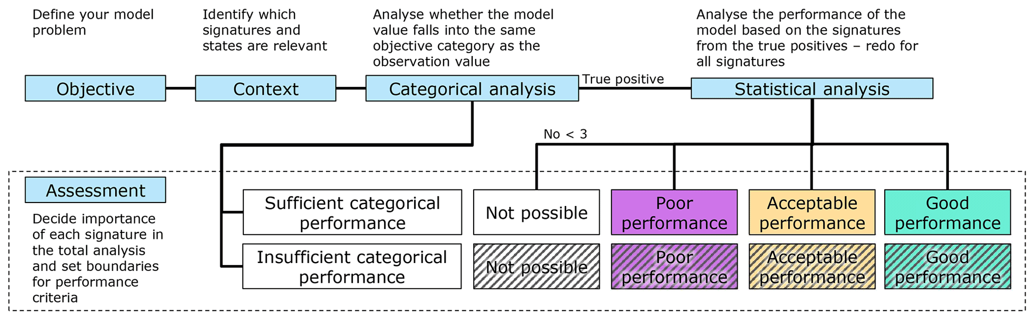
Figure 1 Identified steps (blue boxes) for assessing model performance. With respect to accommodating colour-blindness, the yellow and red colours are changed to orange and purple.

The model adequacy assessment outlined in Fig. 1 does not serve to reduce model uncertainty directly, as is usually the case for calibration methods. Rather, the aim is to assess how well the model is able to replicate reality (by comparing with observations) for defined model objectives. When acknowledging that a model has poor performance for a specific objective in a given area, the end-user may wish to identify the location of the apparent uncertainties. Model uncertainty assessment is a large field, and many terminology frameworks have been suggested in the scientific literature, which are, however, not always perfectly aligned across modelling fields and purposes. In our prior work (Pedersen et al., 2022), we combined the content of two well-cited papers by Walker et al. (2003; focusing on uncertainty locations) and Gupta et al. (2012; focusing on the uncertainty in model structure) into a unified framework explaining the locations of uncertainties present in the semi-distributed integrated urban drainage models, which our work focuses on (i.e. a lumped conceptual rainfall–runoff module that calculates runoff to a distributed, physics-based high-fidelity pipe flow module). Figure 2 is designed to illustrate this uncertainty classification framework in an easy-to-refer-to manner, so that our discussions related to model uncertainty can become clearer and more structured. Specific symbols are used to illustrate context uncertainty (here buildings that are not part of the model), input uncertainty in external forces (here rainfall) and system attributes (here a pipe), model structure uncertainty related to physical attributes (here the network structure), processes (here infiltration), spatiotemporal uncertainty (here a comparison of two hydrographs), equations and computation (here binary sequences), and, finally, parameter uncertainty (here as illustrated by adjusting different parameters on a control board).

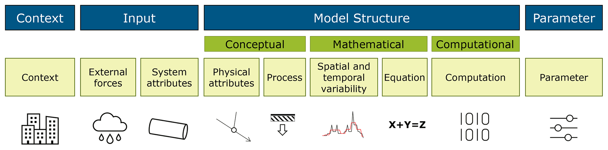
Figure 2 Classification of the location of uncertainties in models, based on Walker et al. (2003) and Gupta et al. (2012). Adapted graphically from Pedersen et al. (2022).

2.2 Model objectives

The utility company defined the objectives based on their interest in model output. The reliability of the operation model is analysed for the following three objectives in this paper: surcharges (water level rises above defined critical levels related to basement flooding), overflows (water levels rise above an overflow weir crest level), and everyday rain events (water levels stay below the top of the pass-forward pipe). These objectives are especially important, as model results are used to support decision-making in relation to future investments. If the model does not mirror physical behaviour adequately, investments can be made based on false premises – potentially leading to human injury or environmental damage that could have been prevented.

A more in-depth description of the objectives that will be investigated in the paper is given below (see the illustration in Fig. 3).

• Surcharges – situations in which peak water levels in manholes rise above defined critical surcharge levels (CSLs). In VCS Denmark, the CSL is generally set at 1.5 m below ground level to mirror the typical level of basements, unless the crest level (CL) or top-of- pipe (TOP) is within the range of 1.5 m. The CSL must not be exceeded more often than every second year in order to provide the optimal service level as required by the utility company (Odense Kommune, 2011).

• Overflow – situations in which the water level rises above the crest level and overflows occur. The overflow criterion only applies to sites equipped with an overflow weir (either internal or external).

• Everyday rain – situations in which water levels are below the top of the pass-forward pipe (TOP) or a crest level (CL) if this is lower. Such events occur for minor rain events that do not lead to exceedance of the pipe capacity, overflow, or surcharge but that occur quite often. In Denmark, the design of a full-flowing pipe is based on rainfall design events for a 2-year return period. The terminology relating to everyday rain is adopted from Sørup et al. (2016) and Madsen et al. (2018).

The above definition of the model objectives means that the water levels in the range between the critical surcharge level (CSL)/overflow crest level (CL) and the top of the pipe (TOP) are not included in the analyses. This is intentional because water levels in this range are often very dynamic due to the limited volume available in the manholes, and model-to-observation fits are thus expected to be poor in this range.

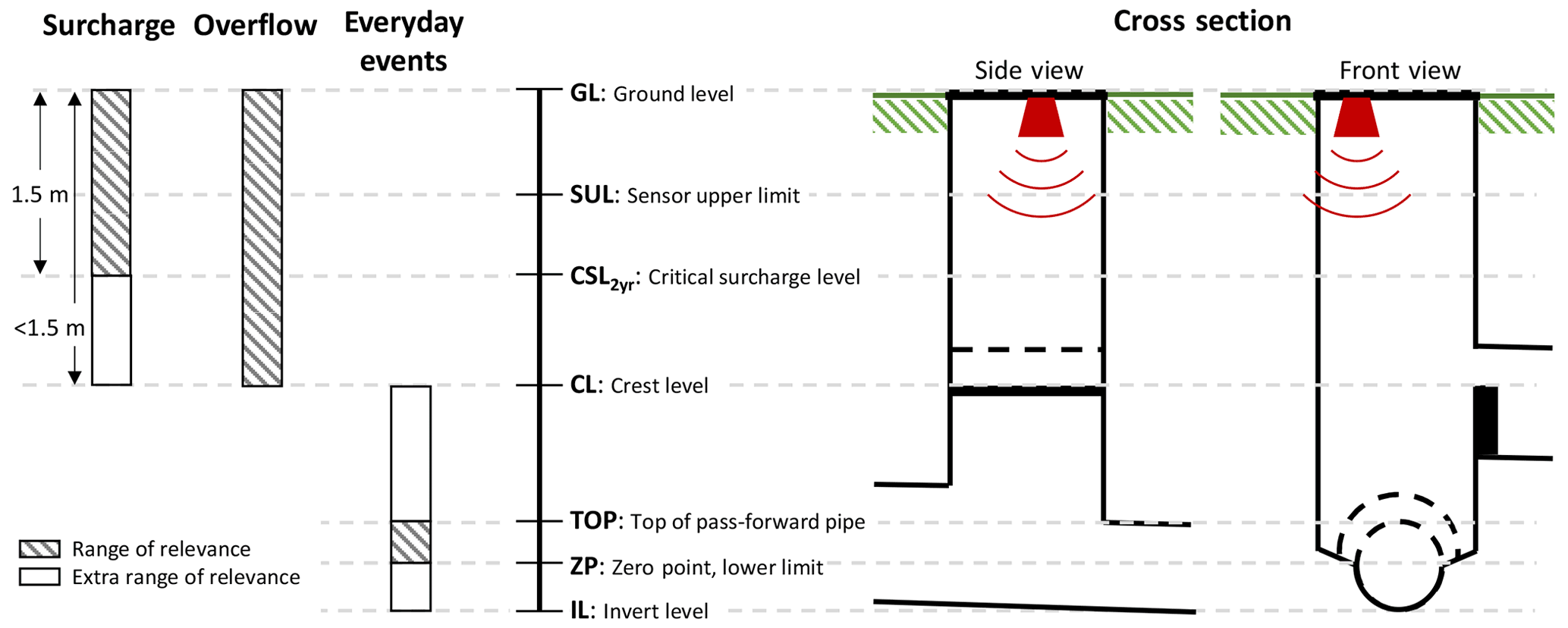
Figure 3 Illustration of the three model objectives (surcharge, overflow, and everyday events) in relation to water levels in the system (left), explanations of the symbols used for specific water levels in the figure (middle), and cross sections through a structure equipped with an overflow weir (right). Overflow occurs for events where the water level rises above the crest level (CL). Surcharge occurs for events where the water level rises above the critical surcharge level (CSL), which is defined as 1.5 m below ground level (GL) – or if the crest level (CL) or the top of pipe (TOP) is within the range of 1.5 m, then that level will be the CSL. Everyday events are when the water levels being observed or modelled are below the top of the pipe (or CL if this level is lower) and above the invert level (IL, or zero point, ZP, i.e. a lower sensor limit if this level is higher).

2.3 Context definition

Methods for handling unrealistic anomalies can be found in the literature (e.g. Clemens-Meyer et al., 2021). For this study, the simple data-cleaning approach by Pedersen et al. (2021b) was applied, using five techniques (low data quality determined by the supervisory control and data acquisition (SCADA) system manufacturer, manually removed data, out of physical bounds considering the specific sensor, frozen sensor signal, and outlier data as assessed by an operator). Erroneous observation data were interpolated up to 5 min and otherwise replaced with NaN (not a number) values.

Since the three model objectives are related to rain-induced events and not dry weather conditions, a time-varying event definition was applied for the time series, with a focus on water levels that are above the water level variations on a normal dry weather day influenced by infiltration inflow (Pedersen et al., 2022). These events were found for the observed and modelled time series, both separately and jointly; the joint events were applied in this study.

2.3.1 Signatures

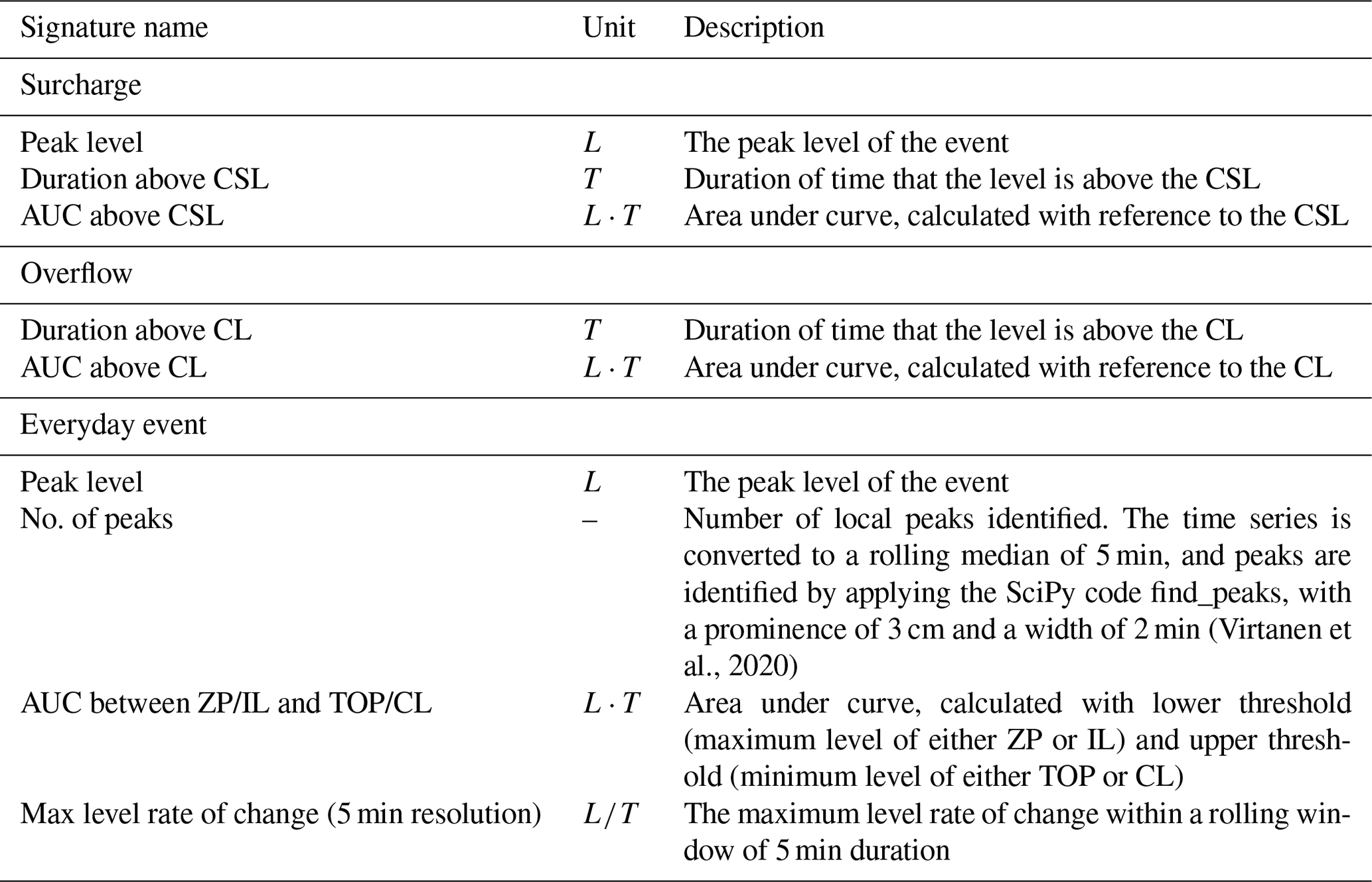
Signatures are metrics that extract specific characteristics of a time series event, as illustrated for water levels in Fig. 4. Peak level, duration, and area under curve (AUC) were previously described in Pedersen et al. (2022). The two first are standard metrics used in common practice, the third (AUC) calculates a surrogate volume for an event from a reference level (similar to the area under a flow hydrograph but with a different unit). Relevant signatures must be selected for each model objective in order to evaluate the model performance. A selection of signatures (Table 1) was based here on an assessment conducted by the author group, including discussion of this topic with a group of utility experts in hydraulic modelling. The relevant signatures for the objective surcharge are peak level, duration above the CSL, and AUC above CSL. Signatures relevant for the objective overflow are duration above CL and AUC above CL. Peak level is not of interest for the overflow objective, and therefore, it is not included. The relevant signatures for the objective everyday events are peak level, number of peaks, the AUC between the zero point (ZP)/invert level (IL), and the TOP/CL (the range of relevance; see Fig. 3) and the maximum level rate of change (5 min smoothing window). These were chosen based on an assessment that they will provide valuable insights into the everyday event. Further analyses could have been conducted to support the relevance, but that lies outside the scope of this paper.

Figure 4 Simple representation of the signatures.

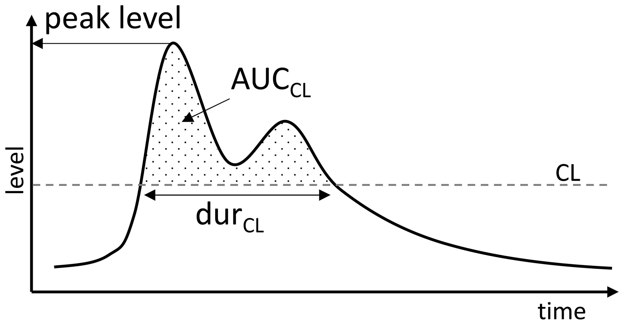
Table 1 Relevant signatures included for the analysis of three defined model objectives. Units are L= for length and T= for time.

2.3.2 Weighting of individual events in the categorical and statistical analyses

A model should, in theory, be able to replicate all measured events. However, in practice, this is often not the case because uncertainties can potentially be identified in several model locations (Fig. 2) and because the system and the sensors can exhibit abnormal behaviour not included in the model set-up. These events, where anomalies occur, constitute an outlier in relation to a model's performance, as the model is not made to handle these issues. Referring to Fig. 2, this would indicate a location of uncertainty in the context area, as the model does not have the primary focus to handle all situations. It is also generally accepted that the model output is very sensitive to the input of rain, in terms of spatial coverage. When an intense storm event only affects a limited physical area, where only few rain gauges are monitoring the rainfall, the corresponding rainfall input may not be correct, generating high degrees of uncertainties in the model grounded in the location input (Fig. 2). This uncertainty may be reduced with rain radar input, but this possibility has not been investigated in this study. The same occurs for the sensors. If the sensor's range is shorter than the water level that it is measuring, then this may affect the time series of the observations, but not necessarily all the signatures would be affected. An upper limit of the sensors may furthermore be exceeded by the water level, and the peak level will reach a limitation and thereby be wrong. However, the signature duration above CL may not be wrong if only the sensor is placed above the crest level. Depending on the importance of the model investigated, quantitative measures of different uncertainty locations can be included in the weights.

In this study, a method was developed to reduce the weighting of individual events in the categorical and statistical analyses in order to acknowledge the uncertainty in model and/or measurements in cases where the model is not expected to fully replicate the measurements. The weights for each event were, for this analysis, calculated based on the following rules.

• Events for which the peak level has reached the upper sensor limitation were given a weight of zero for the signatures, i.e. peak level, AUC above CL, and AUC above CSL.

• Events for which there is a known system anomaly were given a weight of zero for all signatures. Known system anomalies were identified based on manual inspection of the outlier events.

• Events for which the rain input uncertainty is particularly high, quantified by the coefficient of variation (CV) of the rain depth of the rain gauges within a 5 km surrounding (Pedersen et al., 2022), were given a weight from zero to one. The weight w was calculated as $w=\mathrm{1}-\mathrm{CV}$ (for CV≤0.5), $w=\mathrm{0.5}\cdot (\mathrm{1}-\mathrm{CV}$) (for 0.5<CV≤1) and w=0 (for CV>1).

2.4 Categorical analysis

Analysing model performance for specific objectives suggests that events can fall into different categories (e.g. overflow or no overflow). For relevant signatures, the categorical analysis aims to identify, for each event, if observed and modelled results are above or below a given threshold, for example, the crest level for the objective overflow (Fig. 5). If both a modelled and observed event is above the threshold, then the event is categorised as a true positive (TP). If the number of TPs, relative to the false positives (FPs – modelled, but not observed, threshold exceedance) and false negatives (FNs – not modelled, but observed, threshold exceedance), is too low, then the model simulation of the events is not correct, categorically speaking, and the confidence, or trust, in the model is low.

Several metrics can be applied to assess the categorical performance of the model; however, for this analysis, where we are dealing with rare events, the metrics should not include the true negatives (TNs). The metrics chosen is thus the critical success index (CSI; Bennett et al., 2013), which takes the true positives (TPs) compared to all observed or modelled positives (TPs, FPs, and FNs).

$$\begin{array}{}\text{(1)}& \mathrm{CSI}={\displaystyle \frac{\mathrm{TP}}{\mathrm{TP}+\mathrm{FP}+\mathrm{FN}}}.\end{array}$$

For this categorical analysis, the weights introduced above were considered so that events with w<0.5 were disregarded.

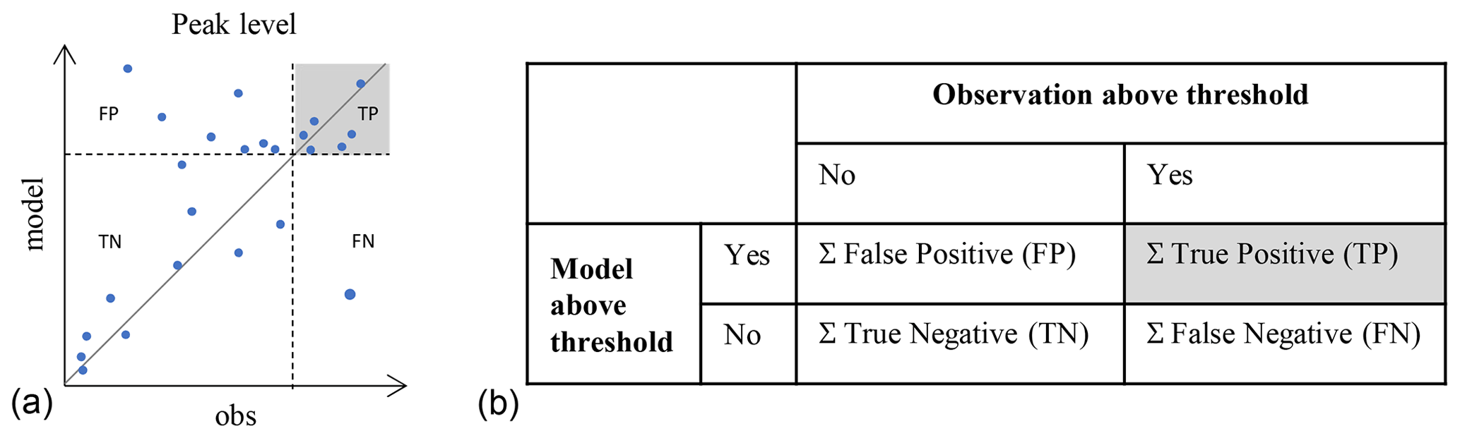
Figure 5 Contingency tables (b) are used to categorise each event according to whether it is above or below a given threshold. The solid line (a) is the 1:1 line, the blue points are the calculated signatures for each event (modelled vs. observed value), and the dotted lines represent the threshold used to distinguish positives from negatives.

2.5 Statistical analysis

The events categorised as true positives can be assessed statistically. Scatterplots of multi-event signature comparisons can be made with observation signature values for each event on the horizontal axis and modelled values on the vertical axis. A 1:1 line indicates the perfect model-to-observation fit (Fig. 6), and three different ways of analysing the scatterplots were assessed in this paper, namely linear regression (Fig. 6, left), an indicator function (Fig. 6, middle), and the normalised root mean square error (RMSE) method (Fig. 6, right).

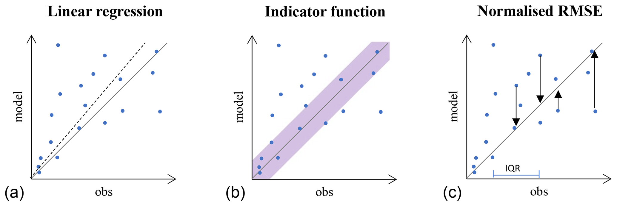
Figure 6 Three methods of statistical analyses of the true positive events, where both simulated and observed values are in the same (true positive) category. Linear regression (a), an indicator function defined using an absolute scale (b), and normalised root mean square errors (RMSEs) are shown (c). The solid lines are the 1:1 lines, and the blue points are the calculated signatures for each event (modelled vs. observed values).

2.5.1 Linear regression

Linear regression is a simple statistical method to assess whether there is a correlation between two variables, in this case the observed and modelled signature values. If there is a cluster along a straight line, then this will indicate a correlation of the two variables. A weighted least squares (WLS) regression model was used to include the individual event weights (see Sect. 2.3.2). A fixed intercept of zero was used, as the theory indicates that this would be the optimal solution. The slope β was found by minimizing the weighted sum of squares (WSSs) as follows (Eq. 2):

$$\begin{array}{}\text{(2)}& \mathit{\beta }\mathrm{from}\min (\mathrm{WSS}\left(\mathit{\beta },w_{\mathrm{e}}\right)={\sum }_{\mathrm{e}=\mathrm{1}}^n{w}_{\mathrm{e}}{\left(y_{\mathrm{m},\mathrm{e}}-y_{\mathrm{o},\mathrm{e}}\mathit{\beta }\right)}^{\mathrm{2}}),\end{array}$$

where y_o is the signature observation value, y_m is the signature modelled value, e is the event number, and w_e is the weight of event e. The model is found adequate if the slope is 1, and a slope different from 1 (and indicated by a dashed line in Fig. 6, left) may suggest there is room for improving the model. In practical terms, the WLS regression was conducted with the Python package, scikit-learn, linear regression with sample weights (Pedregosa et al., 2011).

Four assumptions need to be valid to conduct weighted linear regression, namely linearity (linear relationship between y_o and y_m), homoscedasticity (the variance of the residuals is the same for all y_o), independence (the residuals are independent of each other), and normality (the residuals are normally distributed; Olive, 2009).

2.5.2 Indicator function

The score for the indicator function has a binary output of I. If the event is within the acceptance criteria (AC; Eq. 3; Taboga, 2021), indicated by the purple area in Fig. 6 (middle), then I will have a value of 1 (Eq. 3), and a total score across all events was calculated by considering the weights introduced in Sect. 2.3.2 as follows (Eq. 4):

$$\begin{array}{}\text{(3)}& {\displaystyle }{I}_{\mathrm{AC}}\left(e\right):=\left\{\begin{array}{l}\mathrm{1}\mathrm{if}e\in \mathrm{AC}\\ \mathrm{0}\mathrm{if}e\notin \mathrm{AC}\end{array}\right.\text{(4)}& {\displaystyle }\mathrm{score}={\displaystyle \frac{{\sum }_{e=\mathrm{1}}^n{I}_{\mathrm{AC}}\cdot w_{\mathrm{e}}}{{\sum }_{e=\mathrm{1}}^n{w}_{\mathrm{e}}}}.\end{array}$$

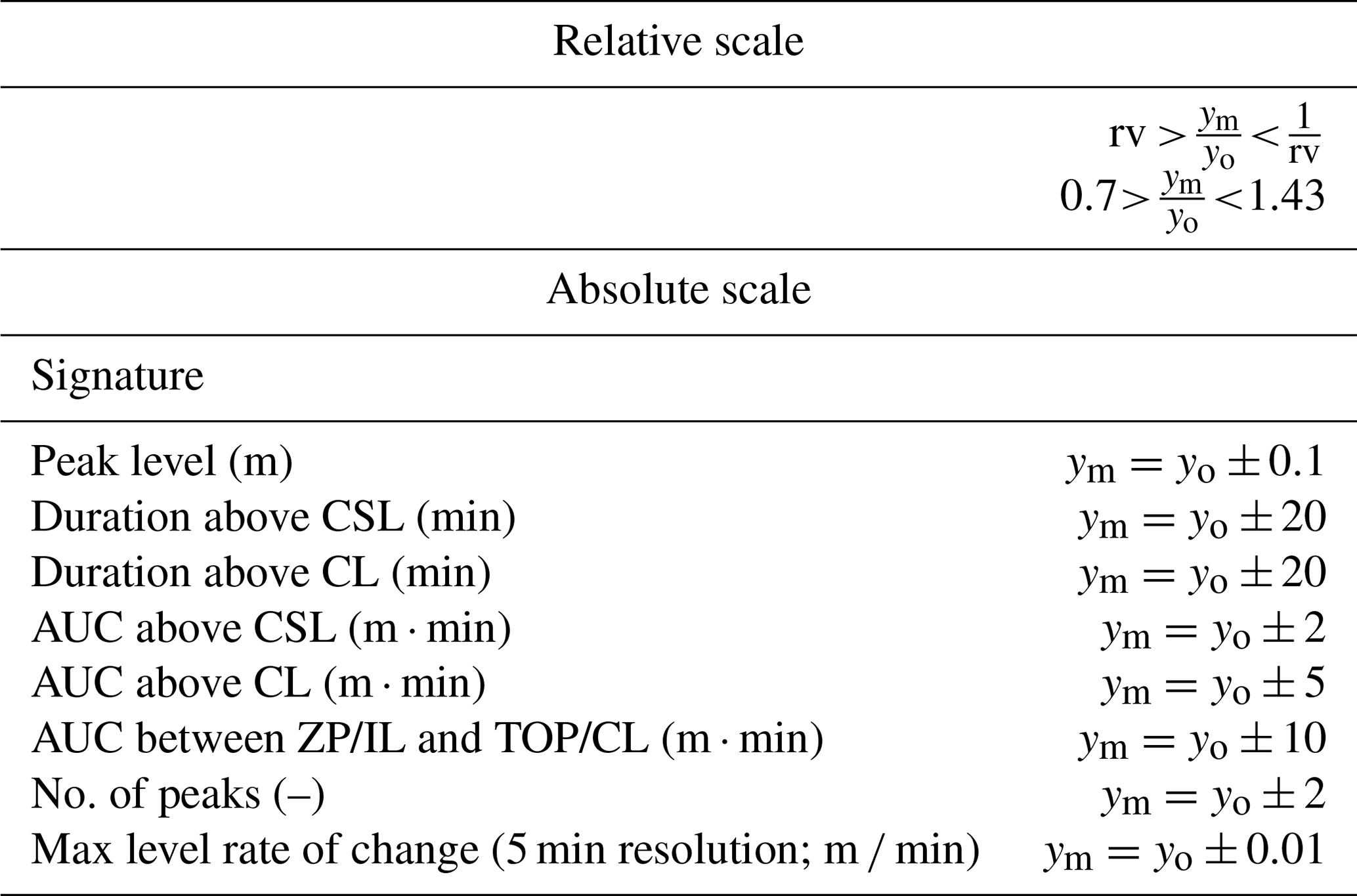
A good comparison gives a value of 1, as all events will be within the indicator function's acceptance bounds. The acceptance bounds were, for this analysis, made by a combination of a relative and an absolute criterion and were, for all sites, assessed to be the same as indicated in Table 2.

Table 2 Values representing the acceptance criteria for different signatures. The acceptance bounds are based on the combination of both the relative and absolute acceptance criteria. The absolute values relate to the 1:1 line, and the relative scale gives the slope range of acceptance. rv is the relative value which is, in this case, set to 0.7, y_m is the modelled signature value, and y_o is the observed signature value.

2.5.3 Normalised RMSE

The RMSE function calculates the vertical distance (of modelled values) to the 1:1 line to find the residuals in the model performance (Fig. 6, right). RMSE is directly related to data and needs to be normalised to be (meaningfully) compared across sites and signatures. This can be achieved by dividing with, for example, the maximum value of the observations or the interquartile range (IQR(y₀)) of the observations (the difference between the 75th and the 25th percentiles). As the maximum value relies on extreme events, it is not considered to constitute a robust normalisation solution, and the IQR was thus chosen, as follows (see Eq. 5):

$$\begin{array}{}\text{(5)}& \mathrm{RMSE}\left(\mathrm{IQR}\right)={\displaystyle \frac{\sqrt{\frac{\mathrm{1}}{n}{\sum }_{e=\mathrm{1}}^n(y_{\mathrm{m}}-y_{\mathrm{0}}{)}^{\mathrm{2}}}}{\mathrm{IQR}\left(y_{\mathrm{0}}\right)}}.\end{array}$$

The smaller the RMSE(IQR) value, the better the model performance.

2.5.4 Score

An individual score (slope, score, or normalised RMSE, respectively) for each signature was calculated, which can be summarised to one score for the following given objective:

$$\begin{array}{}\text{(6)}& \mathrm{Objective}{\mathrm{score}}_{\mathrm{m}}={\displaystyle \frac{{\sum }_{\mathrm{s}=\mathrm{1}}^z{\mathrm{score}}_{\mathrm{s},\mathrm{m}}}{z}},\end{array}$$

where score is the different score functions given by Eqs. (2), (4), and (5), s denotes signature, m is the method (either linear regression, indicator function, or normalised RMSE), and z is the total number of relevant signatures for the given objective. The optimal score is individual for the three methods, and direct comparison is therefore not possible.

2.6 Assessment criteria of the model performance score

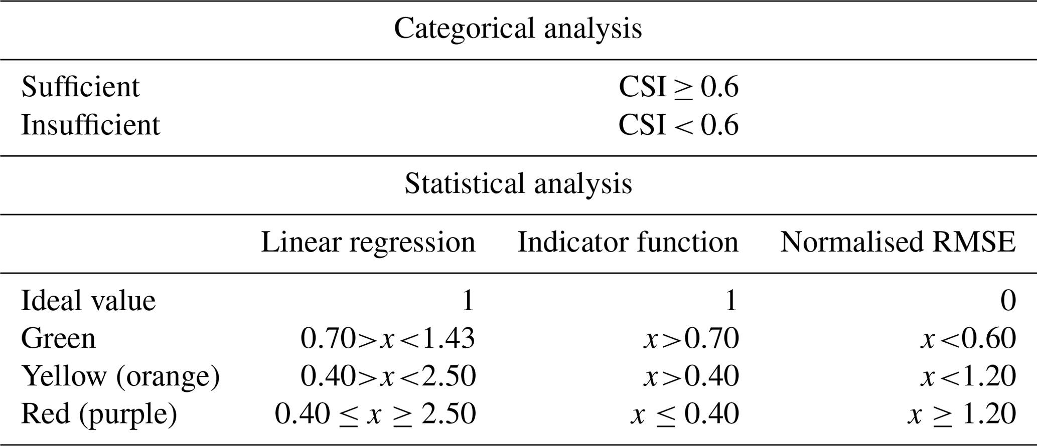
As a last – and illustrative – step, the scoring of the model performance was categorised, as indicated in Fig. 1. The categorical analysis outcome was classified as either sufficient or insufficient, and the statistical analysis outcome was classified by means of a traffic light assessment (green is good performance, yellow (orange) is acceptable performance, and red (purple) is poor performance). The criteria for which score falls into each assessment category were here solely based on the subjective experience from the author group (Table 3). One consideration was not to be too hard on the model, as it is expected that several other factors affecting the weights were not included in the calculations. These distinction criteria can potentially differ, depending on the model objective, and be tuned to yield results that support the end-user's preferences. However, there is limited prior experience with dealing with criteria as such, as the method and the ambition to conduct multi-site analysis is new. Prospectively, future experience with the methods will strengthen the choice of criteria.

Table 3 The criteria for the categorisation of the model performance, solely based on the utility company's preferences. x denotes the output from each method (slope, score, and RMSE(IQR)).

3 Study area, model, and data

The analysis covers two case areas of Bellinge and Dalum, which are in the service area of the utility company, VCS Denmark. The areas are characterised by being suburban areas with minor surface gradients. The urban drainage system analysed is a combined system, and both areas are upstream from a main collecting pipe transporting the combined sewage to the treatment plant. The case areas for this study includes 23 sites with water level meters installed, as highlighted in Fig. 7. The site naming is systematic and includes a reference to where the manhole is located (characters 1–3), which system type it is (character 4; F is a combined system, and R is a rainwater system), a forthcoming number (characters 5–6), an indication (character 7) of whether it is a basin (B), if it is being regulated (R), or if it is an overflow structure (Y), and a further suffix in some cases to indicate the location of this manhole within a larger hydraulic structure. Some sites contain more than one level meter. The normal flow direction of the wastewater is illustrated, as are the combined sewer overflow locations (green dots). In Dalum, there are many ring connections, where the combined sewage can be directed to several catchment areas in the case of high water levels. This is, however, not indicated in the sketch.

The applied model is a semi-distributed “integrated urban drainage model” (Bach et al., 2014). It includes a lumped conceptual rainfall–runoff module that calculates runoff to a distributed, physics-based pipe flow module, computationally carried out in the software MIKE URBAN (DHI, 2020). The model set-up is described in detail in Pedersen et al. (2021b) and is openly accessible. The rainfall–runoff calculations are based on the time–area model (model A) – infiltration–inflow to pipes is not included. The model includes approximately 3500 nodes, and the imperviousness of sub-catchments was calculated based on a categorisation of the surface from satellite data using spectral analysis. Rain input was measured by two rain gauges in the proximity of the study area (Fig. 1). The hydraulic reduction factor was set at 0.9, and the model was run continuously for approximately 10 years (2010–2021), with a time step of 5 s in the pipe flow module. Water level time series from 23 sites in the study area are included in the analyses; these have durations between 2 and 11 years and include between 127 and 2246 rain-induced events, with the event definition described in Pedersen et al. (2022). Observations and model output are in this paper presented in water level time series with a temporal resolution of 1 min.

Further description of sites and models implemented in MIKE URBAN and the Storm Water Management Model (SWMM) are available in Pedersen et al. (2021b) for Bellinge, and Pedersen et al. (2022) provides a description of three sites in these areas of F67F47Y, G73F010, and G71F05R_LevelBasin, including information about the horizontal area of the structure, the levels, crest widths and imperviousness, and total areas.

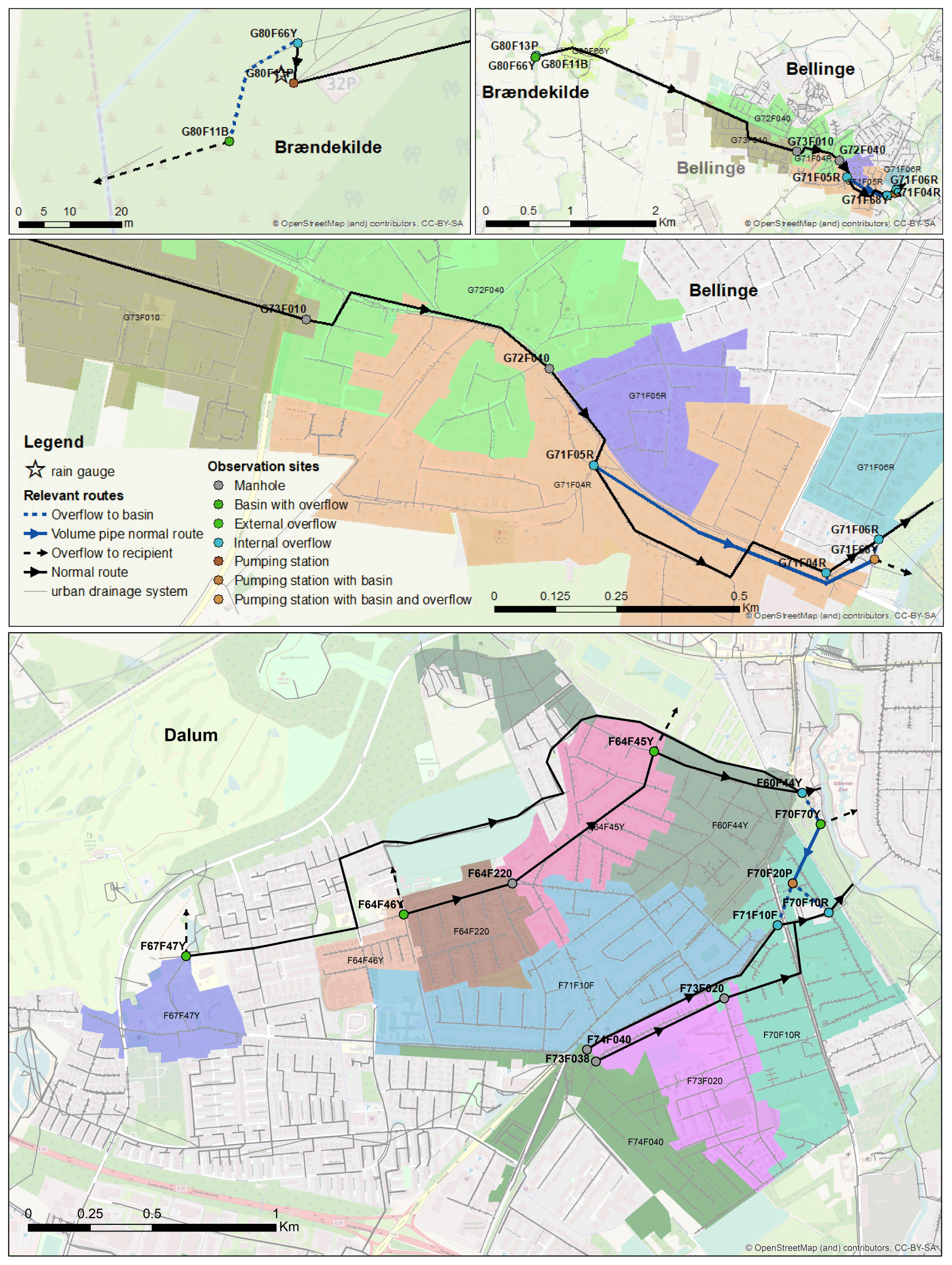
Figure 7 Observation sites in the case areas. Many internal connections between the different areas are present in Dalum, but these are not illustrated in the figure. The node names in the centre of the sub-catchments refer to the connected manholes downstream. The background map is from OpenStreetMap (2022).

4 Results and discussion

4.1 Direct time series comparisons for different objectives

The time series analysed were split into events, as illustrated for six examples of events in Fig. 8. The different events are examples of surcharge, overflow, and everyday events in the different columns, and the rows indicate two different sites (F64F46Y, Fig. 8a–c, and F70F70Y_LevelSump, Fig. 8d–f). Observed water levels (red dots and line) and modelled water levels (blue lines) are plotted, and weights (see Sect. 2.3.2) and signatures related to the specific objectives are shown in the top right-hand corner of each panel. The grey areas illustrate the range in which the peak of the observed and modelled water levels should be in order to be considered true positives and be included in the statistical analysis. Each event can be visually interpreted, and different model replications can be seen for the events. Figure 8e illustrates how the model replicates the objective overflow, even though the model does not replicate the rest of the event. In this specific case, the event is not replicated well below crest level due to a missing global control setting for the pump emptying this site. The opposite is seen for Fig. 8a, where the objective surcharge is not replicated very well (a heavy overestimation of the peak level by the model), but the rest of the event shows better performance. However, this is not critical if we are aiming to figure out the performance for critical surcharge levels. Figure 8d–f clearly illustrate that the lower sensor limitation (zero point, ZP) differs from the invert level (IL). As illustrated in Fig. 8f, the area of interest is limited to the level between ZP and TOP. This also illustrates that, with the given objectives in this paper, the water level range between TOP to CL for site F70F70Y_LevelSump will not be included in the analyses.

In the top right-hand corner of all panels in Fig. 8, the weights of the events are indicated (see Sect. 2.3.2). The term weight rain refers to weights calculated from the spatial rainfall information, and weight obs. refers to weights determined from information about known system anomalies and the sensor upper limitation. Figure 8b and d show a very low weight on the rain, indicating that these events will not be valued highly in the further analysis. Furthermore, Fig. 8d shows that the water level has reached the upper sensor limitation, and the entire event therefore receives a weight equal to 0 for peak level and AUC above CSL. The duration is not affected by the sensor upper limitation, and therefore, this signature will still count in the further analysis of this signature; however, it will still have a weight of 0.23 from the rain gauge uncertainty.

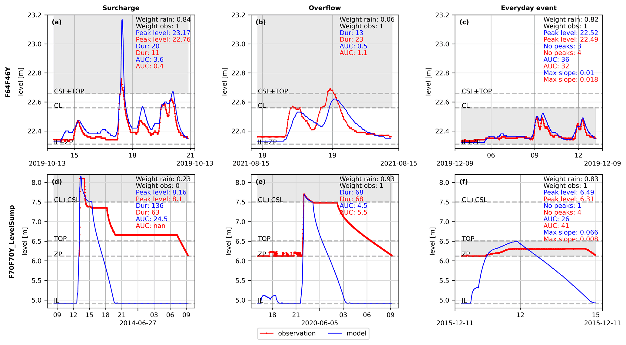
Figure 8 Examples of time series plotted for two sites (rows). F64F46Y (a–c) and F70F70Y_LevelSump (d–f). The objectives are illustrated in the columns as surcharge, overflow, and everyday events, respectively. The values indicated in the top right-hand corner of each subplot indicate the values of the signatures for the three objectives for the modelled event (blue) and the observed event (red). The weights of the rain gauge uncertainty are indicated, in addition to the weight obs., which is a combination of the weights from known system anomalies and indications of whether the sensor reached an upper limitation.

4.2 Illustration of different categorical and statistical scores

To illustrate the procedure of the categorical and statistical analysis, multi-event signature comparison plots are shown for three sites for the objective overflow in Fig. 9. Multi-event signature comparison plots for all signatures and objectives across all 23 sites can be found in the Supplement. Each column in Fig. 9 illustrates a signature, i.e. peak level, duration above CL, and AUC above CL, respectively. The grey areas on the peak level comparison plots illustrate the range of true positives for the objective overflow. The weight of the events is indicated by the coloured scale, where events assigned a weight of 0 (red colour) do not have any influence on the output of the methods. The true positives for the objective overflow are plotted in the last two columns. Important elements are illustrated for the three investigated statistical analyses (see Fig. 6), namely linear regression (with slope as a black dashed line), indicator function (with the purple area defining the acceptance bounds), and the normalised RMSE (with the IQR indicated by vertical blue lines, Q25 and Q75). The score values from the three methods are indicated below each subplot.

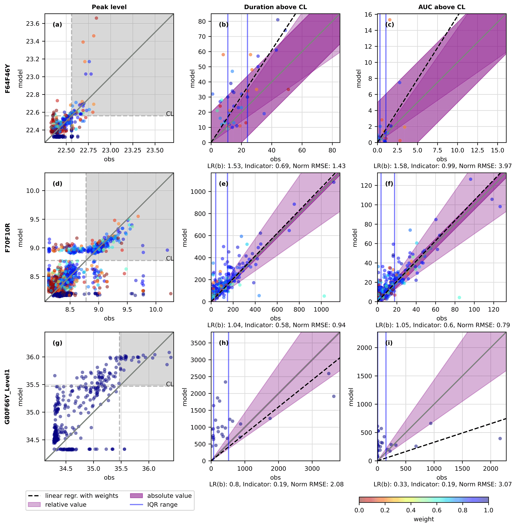
Figure 9 Multi-event signature comparison plots for different sites (rows) and signatures (columns). (a, d, g) The true positive ranges are indicated (grey area), where peak level is above CL for both observed and modelled events. (b, c, e, f, h, i) The true positive events are the only events plotted for the two signatures, where the duration above CL and AUC above CL is seen. An illustration of important elements for the three methods, i.e. linear regression (dashed black line), indicator function (acceptance areas with purple), and normalised RMSE (blue lines indicating IQR), is given. The weight of each event is illustrated with the colour bar. The 1:1 line is plotted with a solid grey line. The score of the statistical methods is indicated below the multi-event signature comparison plot.

For linear regression, Fig. 9c illustrates an event at modelled value 15, which is identified with an uncertain rain gauge input that is given the weight of zero and therefore does not affect the slope. The slope from the linear regression is, on the other hand, affected in Fig. 9i, where a few very large observation values force a low slope gradient even though modelled values seem to be higher at low observation values. For Fig. 9e and f, the slope is very close to the 1:1 line, indicating a close-to-perfect fit with the model. For the indicator function, the purple area illustrates the area where the acceptance criteria are met. Events that are within this area have an indictor value of 1, and their weights are counted in the numerator of Eq. (4), whereas the sum of all the weights are counted in the denominator. The area of acceptance is of great importance, as can be seen for F64F46Y (Fig. 9c), where many events are inside the acceptance criteria, which is also indicated by the score of 0.99. The absolute acceptance criteria are the same for all sites for each signature. It can be discussed if the acceptance criteria should be the same for all sites or if there is site-specific interest that should be taken into account, especially when the utility company sets this evaluation into operation. The IQR are illustrated with the vertical blue lines, and looking at Fig. 9f, a range of approximately 15 m ⋅ min is seen, which is applied to normalise the RMSE. If the error is larger than the IQR, the normalised RMSE will not be within zero to one, and it is therefore difficult to compare values between sites and signatures.

The last site G80F66Y_Level1, in Fig. 9g–i, does not show any weights. For this site, there is only one rain gauge within a 5 km distance of the upstream catchment, and the coefficient of variation cannot be calculated for a single rain gauge. All events thus have the same weight of 1.

4.3 Comparison of methods for statistical analysis

Each categorical and statistical method relies on different metrics, as shown in Fig. 9. In Table 4, the results from for the objective overflow based on the three statistical methods are shown with hatched and colour-coded scorings (Fig. 1; Table 3). Here results are shown only for the 14 sites where overflow is either modelled or measured. The overflow scores are highlighted and were calculated as the average of the two signatures indicated with more transparent colours (Eq. 6). The differences between the methods are large, e.g. where the normalised RMSE method does not generate a very low and optimal score. The first thing to notice is that we have two sites, F70F10R and F71F10F_LevelInlet, where the categorical analysis shows sufficient performance (cells with no hatch; CSI >0.6). From the CSI values provided in Table 4, many values appear above 0.5, indicating that at least half of both modelled and observed positive events were simulated in the same category. However, the threshold for CSI was set to be above 0.6 to have sufficient categorical performance (Table 3), and therefore, it is not enough. Two of the sites, F70F10R and F71F10F_LevelInlet, perform categorically well (no hatched cells) and are acceptable or good for all three statistical methods (yellow/orange and green colours only) when focusing on the objective overflow (Table 4). Looking at G80F66Y_Level1 in Table 4 illustrates that the duration is assessed to be good for the linear regression method. However, when looking at Fig. 9h, a different reality emerges. The variance of data is large, and because of three large observation values below the 1:1 line, the slope is, coincidentally, within the ideal range. The linear regression method could therefore potentially be further improved by including the variance in data in the assessment.

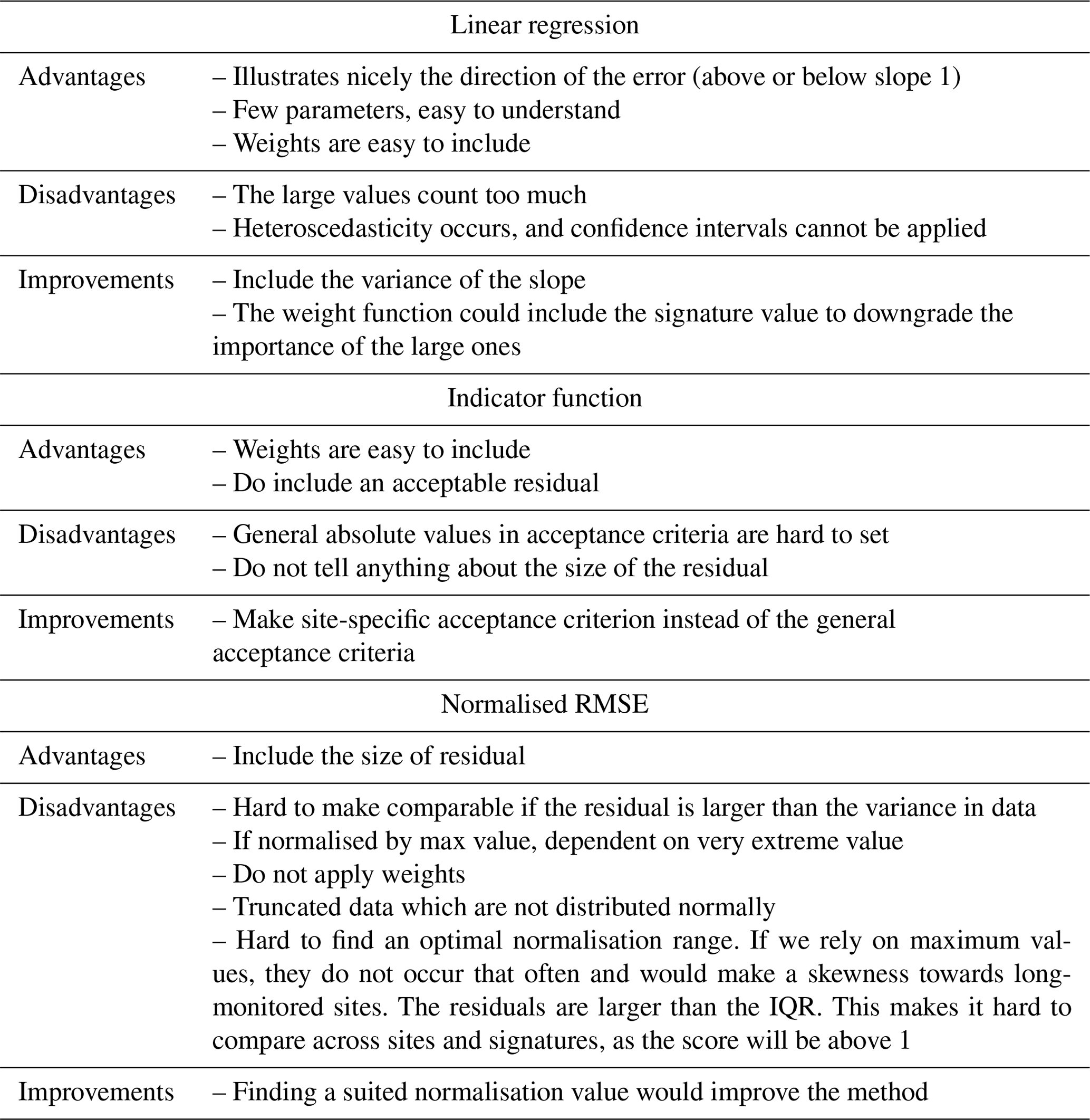
Each method has advantages and disadvantages, as they are based on selected statistical metrics favouring specified features in the modelled and observed signatures. The identified pros and cons for each method are indicated in Table 5, together with suggestions for improvements in the methods.

Table 4 Results from the categorical and the three statistical analysis methods for the objective overflow. Colour-coding as described in Fig. 1 and Table 3.

Table 5 The advantages, disadvantages, and improvements are outlined for the three methods.

4.4 Model performance for all sites and for all objectives

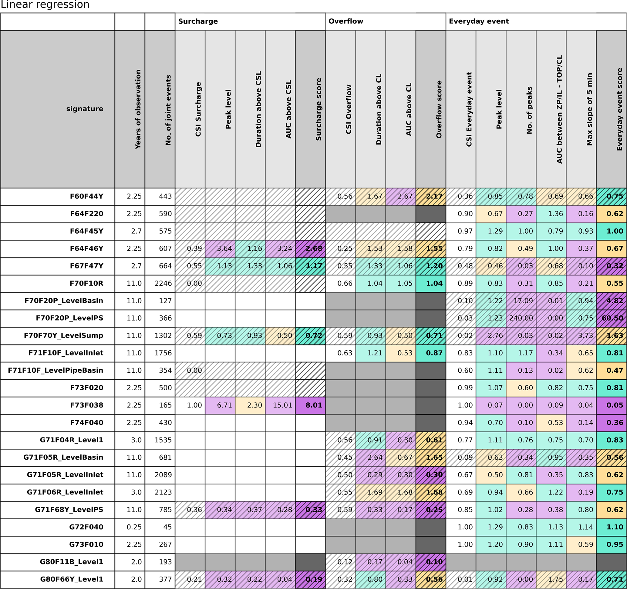
In Table 6, the results for all three objectives using the linear regression statistical analysis method are summarised across all 23 sites. Looking at the performance score for all objectives, it can be easily highlighted where the model performs well for different objectives. What is first seen is that, for many sites, a better performance score is obtained for the objective of everyday events than for the objectives of surcharge and overflow. This is not a surprising result for VCS Denmark, as until now the utility company has compared model results with observations manually. Events falling within the range of the everyday events were much more often applied in comparisons, as they, by nature, occur more often. And when they fit – or detective work showed no more misunderstandings in the model – it was simply assumed that this also applied to the surcharge and overflow events. This was not a correct assumption, as is seen in Table 6. When the model is primarily applied for planning and design purposes, i.e. for the overflow and surcharge, then this is a wake-up call for the utility company to change its practices. The sites furthest upstream in the catchment area (F67F47Y, F64F45Y, F73F038, F74F040, and G80F66Y_Level1; see Fig. 7) generally perform more poorly than the rest of the sites. This can be due to the fact that the outliers observed cannot be averaged-out downstream, also that the upstream structures (pipes and manholes) most often are much smaller in diameter than the structures at downstream sites, and that water level variations are thus most probably more dynamic at upstream sites. In theory, the model should be able to simulate the system just as well in the upstream sites, and there should be an increasing awareness of this issue.

For surcharge, many blank fields are seen in Table 6, as not much data are available for these more extreme events. The categorical analysis shows an insufficient performance for many sites, indicated by a hatched white cell – often meaning that the model simulated a surcharge event that was not observed in reality.

Regarding the different signatures, the number of peaks and the different AUCs generally perform more poorly than the other signatures. The AUC is a combination of both a level and a time unit and can therefore be, due to complexity, harder to simulate, but it could also be that diagnostic tools (Pedersen et al., 2022) can identify where the errors occur so that the model can be improved.

The overall score for each objective was calculated as the average of the relevant signatures (as described in Eq. 6). However, when regression slopes are extreme, as, for example, for the number of peaks for everyday events at the site F70F20P_LevelPS (regression slope is 240), the overall score will naturally be affected. A very low score of, for example, 0.02 will not affect the objective score as much but is naturally an extreme as well. It can be discussed if the objective score should be an average of the relevant signatures, the maximum or the minimum, or if more advanced calculations should be implemented, but no matter what is agreed upon, one must also have an eye on the regression slopes for different signatures and on the uncertainty in these.

The assessment of the traffic light could have been analytically conducted by interviewing several experts or making further analysis. Because the methodology is rather new, as is the signature method that the work is based on, the hypothesis is that experts would not yet be familiar with this analysis, and efforts to obtain input from more experts would thus not be fruitful. For now, this final step was limited to be an assessment based on the authors' experience.

Histograms of the linear regression slopes and potential correlations of these slopes with different catchment characteristics were investigated without finding clear tendencies, and these preliminary investigations are thus placed in the Supplement.

Table 6 Table of scores for linear regression with weighted events. The colours refer to the overall performance score; good (green), acceptable (yellow/orange) and poor (red/purple). The white area is where there are not enough true positives to evaluate a score (no. <3; see Fig. 2). The hatched areas refer to the categorical analysis where too many events are not true positive, meaning that they are not modelled or observed. The grey/black area indicates where analysis is not possible due to physical constraints at the site; for example, not all sites have a crest level, and evaluation of overflow is thus not possible.

4.5 Communication to utilities

This analysis is intended to be applied in the service area of the utility company VCS Denmark for at least 165 sites, and an easy-to-understand overview is therefore needed. To communicate the performance score, maps will be generated because these provide a good overview of performance in relation to where the sites are located (see the example in Fig. 10). Together with score tables (Table 6) and multi-event signature comparison plots (Fig. 9), these will provide a strong basis for communication concerning the reliability of models and a basis for improving the models and the attribute representation of the physical assets. Performance scores for the three statistical methods can be found in the Supplement, together with performance maps for all objectives using the linear regression method.

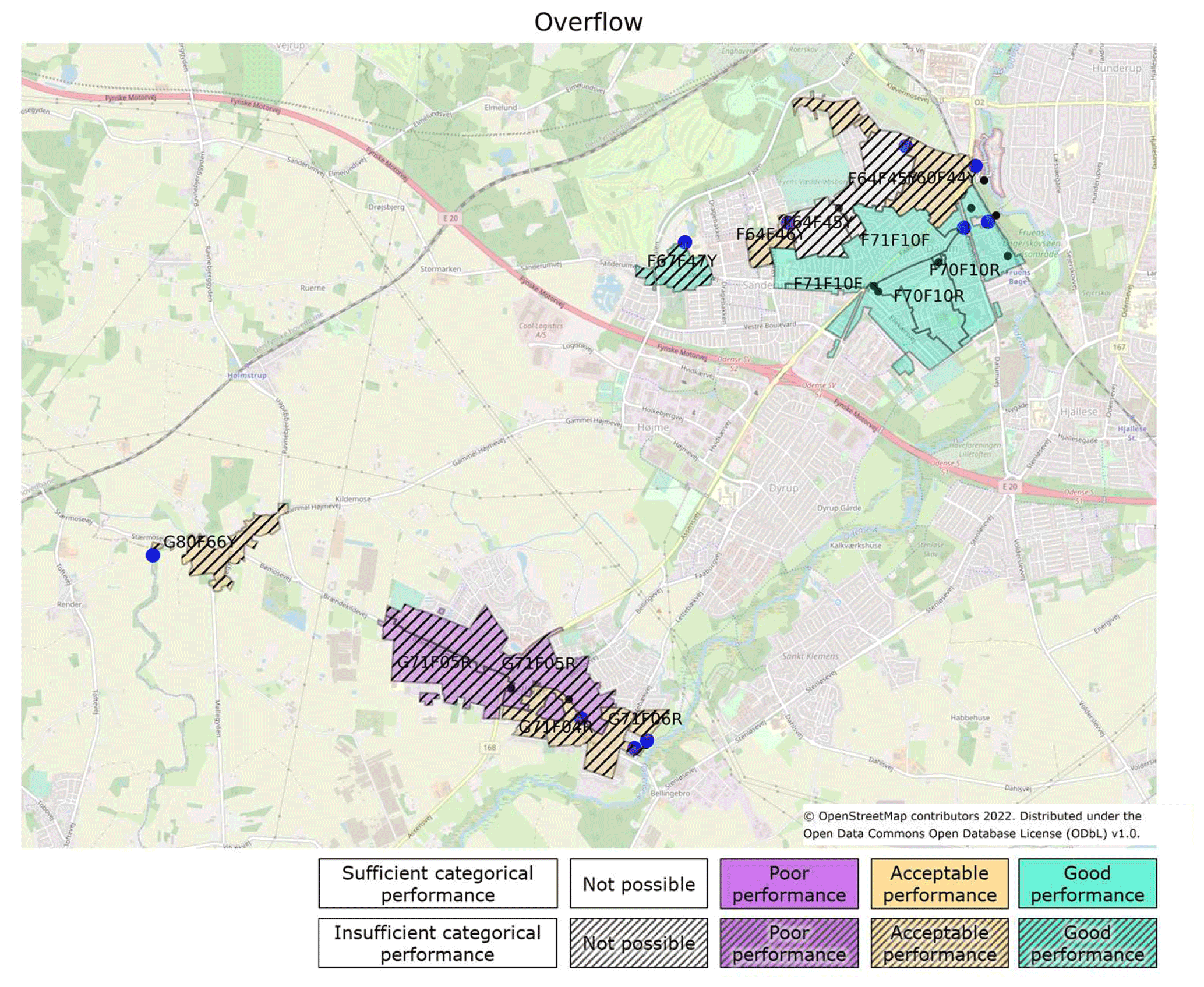
Figure 10 Map of the performance for overflow using the method of linear regression. The upstream catchment area of the site is mapped, and the naming in the catchment refers to the overflow structure that is mapped. The catchment area represents the case areas. The urban areas in between the catchment areas are not connected to the case areas, as they have a separate storm water system. Background map is from OpenStreetMap (2022).

4.6 Useful models?

With increasing digitalisation, where the amount of observation data increases and operational simulation models in digital twins need to be accurate (Fuertes et al., 2020; Karmous-Edwards et al., 2019), the modelling community – across practice and research – needs to discuss how we evaluate whether the simulation models are sufficient for a given task. We suggest, in this paper, a structured methodology for model evaluation, in which there is room for further improvement. How do we, for example, obtain a variety of sensor types incorporated into the framework? In this paper, we furthermore introduce weights to consider input-dependent uncertainty that affects our models, but how can other uncertainty contributions, as described in Fig. 2, be considered in an evaluation, and how can the assessment be used to guide model improvement? In Pedersen et al. (2022), we showed, for example, that soil moisture (which is not included as a model state in the simple rainfall–runoff model from paved areas used and thus can be denoted a surrounding state that is outside the model context) had a systematic impact on the results of the model-to-observation comparison. Soil moisture variability is in the present work not included in the weighting of events, but we could discuss if it should be, or if its influence is better addressed by using a more complex rainfall–runoff model formulation. This may end up in an assessment that there is still residual parameter uncertainty, and we then first suggest performing aa responsibly calibration, as, for example, Deletic et al. (2012) also suggest.

5 Conclusions

Large, detailed, distributed simulation models are widely applied in utility companies. When routinely comparing model results with in-sewer-level measurements from an increasing number of sites, uncertainties previously not realised become visible. The slightly provocative question (how useful are the models then?) highlights the need for methods to systematically assess and investigate model performance. The herein-developed assessment method focuses on highlighting and potentially reducing uncertainty contributions related to (spatially distributed and detailed) system attributes based on the following five consecutive analysis steps: objective identification, context identification, categorical analysis, statistical analysis, and assessment. The method is based on hydrologic and hydraulic signatures, which are metrics extracting certain characteristics of (modelled and measured) time series events. Three model objectives were identified for this study, namely surcharge, overflow, and everyday events, and relevant signatures for each of these objectives were determined. Three methods of multi-event statistical analysis of signatures were furthermore proposed and investigated, i.e. linear regression, an indicator function, and a normalised RMSE method. The results highlighted the differences between the statistical methods but also areas in which further improvements can be made, notably including tests for statistical significance, inclusion of site-specific assessment criteria, and normalising performance scores across methods, objectives, and sites. The final step includes a signature-based assessment for each measurement site with sufficient or insufficient categorical performance and for true positive events also with good, acceptable, or poor statistical performance. Individual events were weighted in the statistical analyses by acknowledging uncertainty due to spatial rainfall variability in the proximity of the site, known system anomalies, and sensor limitations.

A case study covering 23 sites in two areas was conducted using the developed framework, which highlighted a number of model uncertainties for certain sites. For the objective overflow, only three among 14 investigated sites were categorised as exhibiting sufficient categorical performance, whereas the remaining 11 sites had too many events where the observed and modelled signatures fell into different categories. Generally, the model performed better for everyday events, compared to surcharge and overflow events, which is not surprising due to the previous tradition of the model validation in the local utility company (VCS Denmark). With the developed method, the models are useful for some signatures but clearly inadequate for others, especially for some sites. Further improvements may include a general assessment of the performance criteria and more elaborate statistical analysis, as suggested in the paper. Our results point to a general need for more research on model performance and error detection methods that can be applied when comparing simulation results from large, detailed, distributed urban drainage models with observations from tens, hundreds, and perhaps thousands of sensor locations.