the Creative Commons Attribution 4.0 License.
the Creative Commons Attribution 4.0 License.
 | 21 Nov 2022
Technical note: A sigmoidal soil water retention curve without asymptote that is robust when dry-range data are unreliable
Gerrit Huibert de Rooij
In a recently introduced parameterization for the soil water retention curve (SWRC) with a sigmoid wet branch and a logarithmic dry branch, the matric potential at the junction point of the sigmoid and the logarithmic branch (hj) was a fitting parameter, while that at oven dryness (hd) was derived from the fitting parameters. The latter is undesirable, especially if reliable data in the dry range are limited. Therefore, an alternative is presented in which shape parameter α instead of hd is a derived parameter, and hd can be fitted or fixed. The resulting relationship between α and hj is such that it prevents correct fits for hj. Fortunately, an expression for hj is found that allows it to be replaced by α as a fitting parameter. The corresponding parameter space is well behaved and has fewer internal bounds defined by restraining relationships between parameters than the space for hj as a fitting parameter. The few available values of hj in the literature are in line with those according to the new expression. The reformulated SWRC is fitted to data of 21 soils by shuffled complex evolution. The paper gives the main features of an accompanying open source fitting code. The curves fit the data well, except for some clayey soils. A theoretical value of hd performs well for a wide range of soils. The new SWRC simplifies to an earlier junction model of the SWRC based on a well known power-law SWRC if α is very large.
- Article
(2413 KB) - Full-text XML
- BibTeX
- EndNote


Recently, de Rooij et al. (2021) proposed a closed-form expression for the SWRC (soil water retention curve) with a distinct air-entry value, like the SWRC proposed by Ippisch et al. (2006), a sigmoid shape in the intermediate range according to van Genuchten (1980), and a logarithmic dry branch terminating at a finite matric potential hd (L) at which the soil was oven dry, with the water content essentially zero. The volumetric water contents and derivatives of the sigmoid and logarithmic branches were matched at the matric potential of their junction according to Rossi and Nimmo (1994). The rationale for developing the function was to preserve the desirable sigmoid shape of van Genuchten's (1980) curve while removing the physically unrealistic asymptote at some non-zero residual water content (Du, 2020), eliminating the non-converging integral of the SWRC for commonly occurring parameter values (Fuentes et al., 1991), and avoiding the detrimental effect of the non-zero slope at saturation on hydraulic conductivity near saturation (Durner, 1994; Assouline and Or, 2013; Wang et al., 2022).
Erroneous measurements in the dry range can lead to unrealistically low values of the matric potential at oven dryness, hd (de Rooij et al., 2021). Unfortunately, hd was not fitted independently but expressed as a function of other parameters that were fitted. Data in the dry range can be unreliable due to lack of equilibrium or other causes (Bittelli and Flury, 2009; Solone et al., 2012). If they are, it would be helpful to fix hd at a reasonable value, e.g., −106.8 cm H2O (Schneider and Goss, 2012), and either give the unreliable data points a lower weight during the fitting process or remove them altogether. An SWRC with improved behavior in the dry range even if dry-range data are scant can help improve the behavior of Richards' solvers (e.g., SWAP Soil Water Atmosphere Plant, 2022; Šimůnek et al., 2016), be useful to improve conceptualizations of the soil reservoirs in large-scale hydrological models (e.g., Lawrence et al., 2019), and for investigating dielectric properties of dry soil and associated soil backscatter (Ferré and Topp, 2002; Davis and Annan, 2002).
This note presents an alternative to de Rooij et al.'s (2021) model in which hd is a fitting parameter. In doing so, it uncovers the peculiar behavior of shape parameter α (L−1), which makes it essentially impossible for any fitting algorithm to avoid a local minimum with very inaccurate parameter values. The main objective is therefore to elucidate the behavior of α and formulate a version of de Rooij's (2021) SWRC that has hd as a fitting parameter but avoids the difficulties caused by the behavior of shape parameter α.
In the testing phase, it was found that a commonly used convergence criterion used in parameter optimization did not necessarily give the best parameter values if the objective function was challenging. The second objective is therefore to present a parameter fitting algorithm that employs multiple convergence criteria, and optionally explores the parameter space prior to the fitting operation to reduce the search area during fitting. The corresponding open source code for fitting the improved SWRC is provided.
De Rooij et al. (2021) introduced a unimodal model for the SWRC by combining those of Rossi and Nimmo (1994) and Ippisch et al. (2006), dubbed “RIA”.
Here h denotes the matric potential in equivalent water column (L), subscripts “d” and “ae” denote the value at which the water content reaches zero and the air-entry value, respectively, and subscript j indicates the value of h at which the logarithmic and sigmoid branch are joined. The volumetric water content is denoted by θ, with the subscript “s” denoting its value at saturation. Parameters α (L−1) and n determine the shape of the sigmoid branch (van Genuchten, 1980), while parameter β does so for the logarithmic branch. By assuming that for h≤hj, all water is adsorbed and for h>hj, the adsorbed water content is equal to θ(hj), the total water content can be partitioned in a capillary water content θc and an adsorbed water content θa.
By requiring the derivatives of the sigmoidal and logarithmic branches to match at hj, parameter β can be expressed in terms of the other parameters (de Rooij et al., 2021).
Using this expression to eliminate β from the equality that arises when the values of both branches are matched at hj, the resulting expression can be solved for α to establish hd as one of the fitting parameters. The expression can also be found by rearranging Eq. (9) of de Rooij et al. (2021).
The five fitting parameters are hae, hj, hd, θs, and n. Equation (3) is only valid if the bracketed term is positive. This is the case if the following criterion is met:
Many soils for which SWRCs of van Genuchten (1980) or de Rooij et al. (2021) are fitted have values for α between roughly 0.001 and 0.3, with sandy soils generally having higher values than fine-textured soils (e.g., de Rooij et al., 2021). When hd is fixed at −106.8 cm H2O, α is a function of n and hj only. Its contour map is depicted in Fig. 1. De Rooij et al. (2021) reported four soils with data sets without suspect data points above pF 3 for soils with n>1.2 (soils 1142, 1143, 2110, and 2126, all sands or loamy sands). De Rooij et al.'s (2021) values of α and n for these soils give values of hj that are all larger (closer to zero) than −150 cm, which is unrealistic. For soil 2126 the value even exceeds hae, which is not physically acceptable.
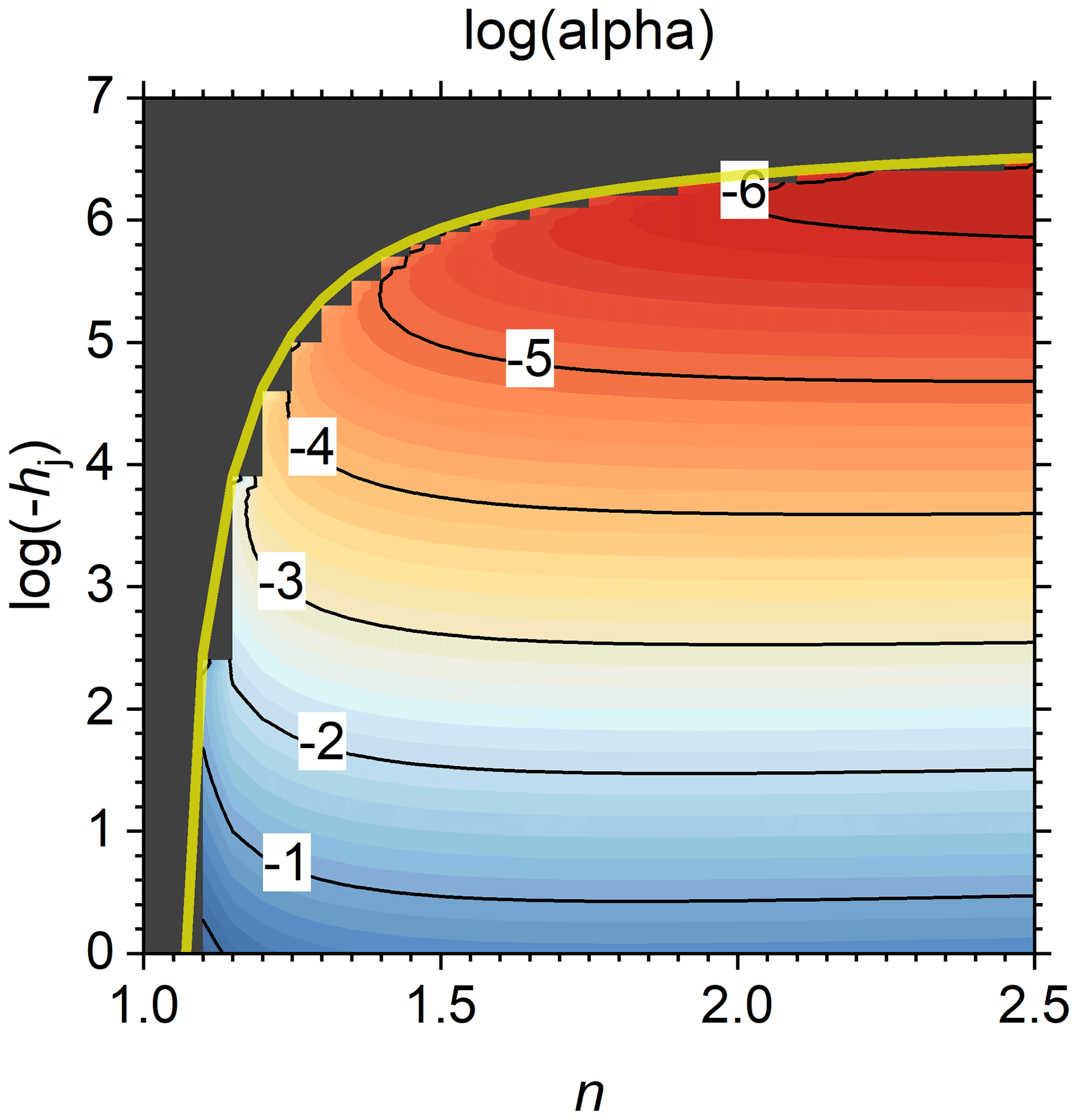
Figure 1The logarithm of shape factor α (cm−1) as a function of shape factor n and the matric potential at the junction point hj (cm H2O) according to Eq. (3), with hd fixed at −106.8 cm. The labels of the contour lines represent log(α). The transparent yellow curve is the limit of the valid domain according to Eq. (4). The black area is the invalid part of the domain.
It therefore appears from Fig. 1 that plausible combinations of α and hj are not feasible, but Eq. (3) reveals that the relationship α(hj) is non-monotonous. A combination of large values of both α and hj is possible in a band too narrow to be visible in Fig. 1, located immediately below the maximum allowed value of hj, marked by the transparent yellow curve in Fig. 1. In that band, α goes to infinity when hj approximates its limiting value defined in Eq. (4) (Fig. 2). The partial derivative of Eq. (3) with respect to hj is as follows:
The value of α is at its minimum where its derivative is zero. According to Eq. (5), this condition is met when the following equality holds:
Because Fig. 1 shows that realistic values of α require excessively low values of hj in much of the parameter space, it may be better to use Eq. (6) to set a lower limit on the permissible values of hj as follows:
Figure 3 shows the band of valid values of hj enveloped by the limits set by Eqs. (4) and (7). A large part of the parameter space between these limits of hj has an excessively large . Finding the optimum will therefore be very difficult for any parameter fitting algorithm. But if the lower limit is not enforced, trial fits showed that the shuffled complex evolution algorithm (SCE, Duan et al., 1992, 1993) consistently ended up in the region of Fig. 1 corresponding to the area below the lower limit in Fig. 3.
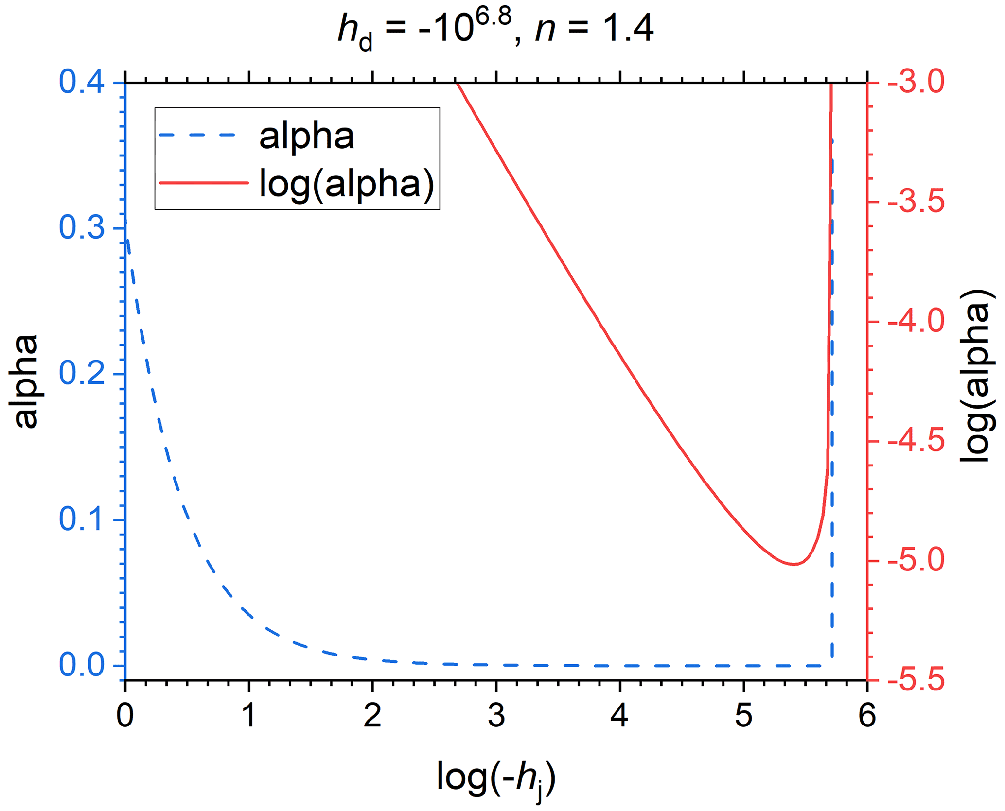
Figure 2A transect of Fig. 1 for n=1.4 that shows the sharp increase of shape factor α (cm−1) as the matric potential at the junction point hj (cm H2O) reaches its physical limit defined in Eq. (4).
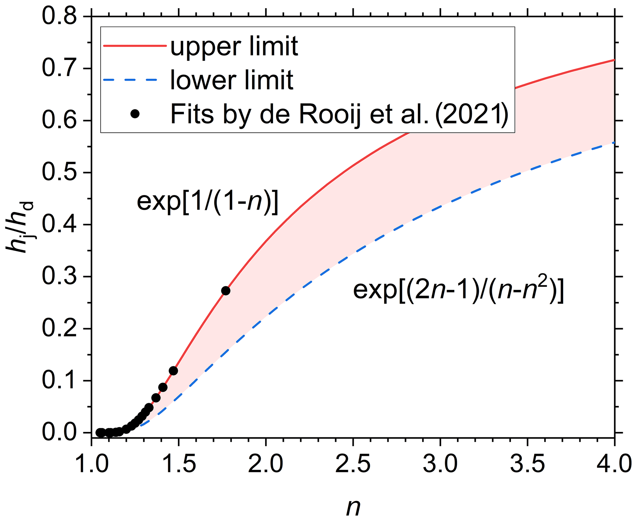
Figure 3The limits imposed on the matric potential at the junction point hj (scaled by the matric potential at oven dryness hd) by the requirement that shape factor α be positive (upper limit) and by the minimum value of α for any specific value of n (lower limit). The shading indicates the area with plausible parameter combinations. The dots represent de Rooij et al.'s (2021) fits of Eq. (1) with α instead of hd as a fitting parameter for 21 soils.
De Rooij et al. (2021) already fitted Eq. (1) with α instead of hd as a fitting parameter and without any restrictions other than minimum and maximum values imposed on any of the fitting parameters. By calculating hd from the fitted values of α, n, and hj according to their Eq. (10), it was possible to see if their fits fell within the limits defined above. Figure 3 shows that the values of all 21 soils fell on the upper limit. This opens the possibility to eliminate hj as a fitting parameter and replace it by its upper limit. This leads to the following additional equation augmenting Eq. (1):
Combining Eq. (8) with Eq. (3) leads to an infinite α, consistent with Fig. 2. But Fig. 2 also shows that a minute change in hj (much smaller than a realistic number of significant digits would be able to represent) allows α to vary beyond the range of values reported in the literature. In other words, if, for given values of hd and n, hj is determined from Eq. (8), α can vary over its entire range. It is therefore better to treat α as a fitting parameter and hj as a derived parameter, by replacing Eq. (3) by Eq. (8). This has the added advantage that the entire parameter space defined by the minimum and maximum values of the fitting parameters is valid, provided the physical and mathematical limits of each parameter are respected, and the fitted or fixed value of hd is smaller (more negative) than hae.
In the limit as α approximates infinity, the expression for the sigmoid branch of the SWRC simplifies to the power law proposed by Brooks and Corey (1964).
It can be easily shown that both the values and the derivatives of the dry and the wet branch match at hj if Eq. (9) is used for the latter. Equation (9) establishes that Rossi and Nimmo's (1994) junction model (without the parabolic smoothing near saturation that Madi et al. (2018) showed to be detrimental to the hydraulic conductivity function) is a special case of the RIA parameterization. Incidentally, this implies that Brooks and Corey's model (1964) is a special case of that of Ippisch et al. (2006).
If Eq. (8) replaces Eq. (3), the fitted value of α no longer ensures continuity at the junction point. The ensuing continuity gap can be closed by applying a correction factor c to the value of hd used in the logarithmic branch as follows:
The correction factor c is defined by the following expression, which is found by replacing hd in Eq. (1) by (1+c)hd, requiring the logarithmic and sigmoid branches of Eq. (1) to be equal at hj, and replacing the ratio in the resulting equality by exp[1/(n–1)] according to Eq. (8).
In the expression for β, hd appears indirectly. Its value should not be corrected there because β ensures continuity of the derivatives only if its expression is not modified. Trial calculations showed that c is negligible, except when both α and n are small.
Rossi and Nimmo (1994) fitted hj values for their parameterization of the SWRC between and cm H2O for seven soils, with only the one clayey soil having a value more negative than cm H2O. Tuller and Or (2005) tentatively set the matric potential at which the capillary-bound water content becomes negligible −105 cm H2O, based on data from a sand mixture and six soils that mostly overlap with those of Rossi and Nimmo (1994) (Or and Tuller, 1999). Beyond this there is little guidance on the value of hj in the literature. When Eq. (8) is used, such guidance is not necessary. The map of hj as defined by Eq. (8) in Fig. 4 shows that for n below 1.4, hj is very sensitive to the value of n. For n>2, log(−hj) is roughly proportional to log(−hd) for a given value of n. When hd is close to −106.8 cm H2O (Schneider and Goss, 2012), values of hj in the range of those reported in the literature occur for n≥1.25.
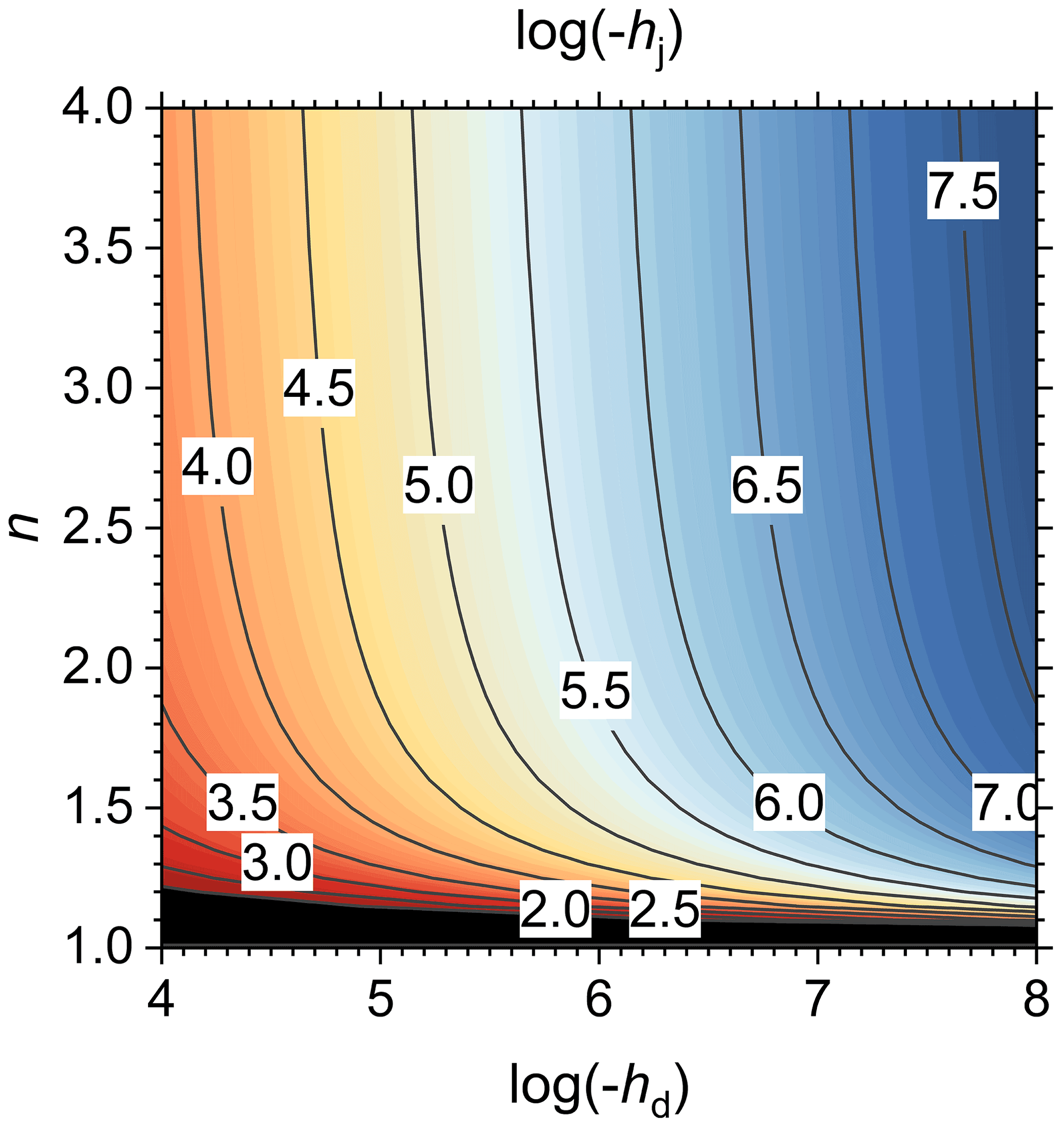
Figure 4The logarithm of the absolute value of the matric potential at the junction point (hj, cm H2O) as a function of the matric potential at oven dryness (hd, cm H2O) and shape factor n, according to Eq. (8). The labels of the contour lines denote log(−hj). In the black region, cm.
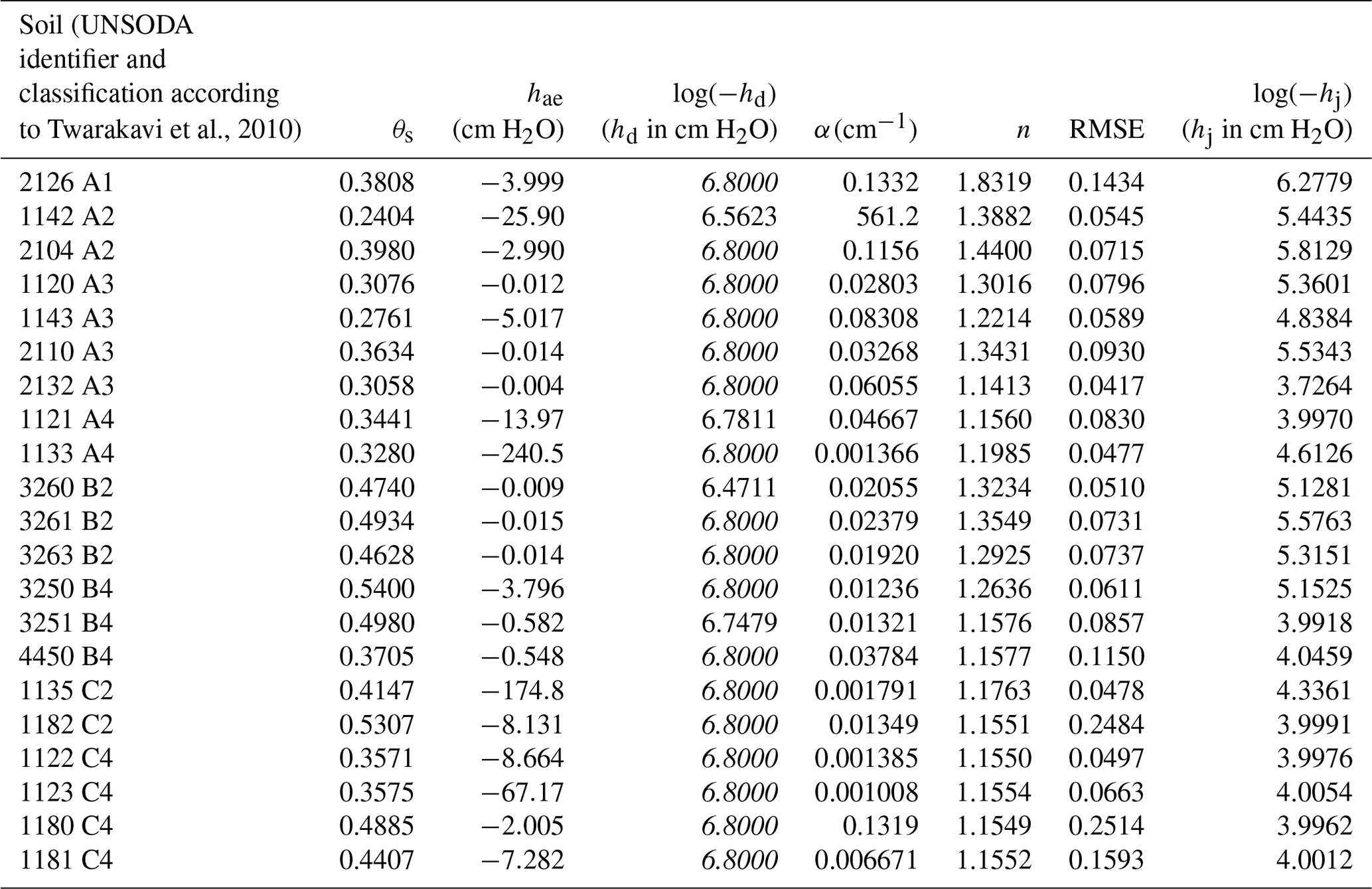
Table 1Fitted parameter values and the root mean square error (RMSE) of the best fits for 21 soils. The corresponding values of the derived parameter hj are given as well. If parameter hd was fixed during the fitting operation, its value is denoted in italic font.
For completeness, the multimodal version of Eq. (1) is provided as well. The multimodality is limited to the sigmoid branch, so that the multimodal SWRC has only one value for hj. Because Eq. (8) allows only a single value of n in that case, only α can be varied between the constituting sigmoid curve sections.
For brevity, the following function was introduced in Eq. (12):
Here, k denotes the modality, wi is the weighting factor (adding up to one) of the ith constituting curve, and αi (L−1) its shape factor. The expression for the multimodal βm is found be setting the derivatives of the logarithmic and the sigmoid branch equal at hj and invoking Eq. (8).
Function G is defined as follows:
The continuity correction factor cm can be found by requiring that the logarithmic and sigmoid branch join at hj.
Above, the subscript “m” is used to distinguish multimodal versions of β and c from their single-mode equivalents.
3.1 Selected soils
The SWRC has five fitting parameters: θs, hae, hd, α, and n. These were fitted to data of the 21 soils selected from the UNSODA database (Nemes et al., 2001; National Agricultural Library, 2015) by de Rooij et al. (2021), with hd either fixed at −106.8 cm H2O, or its lower limit set at that value. These soils cover a wide range of textures (see Madi et al., 2018 and de Rooij et al., 2021 for details). At the time the database was created, the pressure plate apparatus was widely used in the dry range. Therefore, the standard deviation (SD) of the matric potential of any data point with cm H2O was set to half its value, thereby drastically reducing its weight in the objective function. The SD of h for cm H2O was set to 1.0 cm, and that for h=0 at 0.05 cm. The SD for the volumetric water content was set at 0.01 when h=0, and to 0.02 otherwise. The sample height was set to zero for cm because the variation in the water content can be neglected at low matric potentials. For h=0 cm, it was assumed that the water pressure in the sample was positive everywhere, or that the porosity was measured. In both cases, there is no effect of the matric potential on the local water content, hence the sample height was set to zero to reflect this. For the intermediate values of h, the sample height was set to the value specified in the UNSODA database. If a sample height was not reported, it was set to 3.0 cm.
3.2 Parameter fitting
The parameters were fitted using the SCE algorithm (Duan et al., 1992, 1993), implemented in Fortran in a code that accompanies this paper. The most important features of the code are summarized here. The code itself, further details of the code and the algorithm, and a user manual can be downloaded (de Rooij, 2022). For each case, the code performs three optimization runs by minimizing the objective function: the root mean square error (RMSE) of the differences between fitted and observed volumetric water contents, weighted according to the error standard deviations of the observed matric potentials and corresponding water contents provided on input, as detailed by de Rooij (2022).
Ten convergence criteria are evaluated. Criteria 1 and 2 take into account the results of the last few shuffles. The number of shuffles considered is twice the number of fitting parameters or an internally set number (5), whichever is larger.
-
In the best fits from the last set of shuffles, the range of a parameter exceeds neither the absolute nor the relative user-specified tolerance.
-
In the best fits from the last set of shuffles, the range of the objective function does not exceed its absolute user-specified tolerance.
-
The parameter range in the final complexes does not exceed the maximum internally set permissible value.
-
The volume of the hypercube enveloping the final complexes does not exceed the maximum internally set permissible value.
-
The parameter range in the most successful complex (minus the point with the highest RMSE) does not exceed the internally set maximum permissible value.
-
The volume of the hypercube enveloping the most successful complex (minus the point with the highest RMSE) does not exceed the internally set maximum permissible value.
-
A parameter does not exceed both the absolute and the relative user-specified tolerance in the final complexes.
-
A parameter does not exceed both the absolute and the relative user-specified tolerance in the most successful complex (without the point with the highest RMSE).
-
The change of the objective function between consecutive shuffles does not exceed the user-specified tolerance.
-
The root mean square error of the fit does not exceed a user-specified tolerance.
A relative improvement criterion similar to criterion 9 is often used as the sole criterion (e.g., in the R-package SoilHyp, Dettmann, 2021). Criteria 1, 3, 5, 7, and 8 are evaluated separately for each parameter. Convergence is achieved when no more than a user-prescribed number of these criteria failed for any of the parameters. The code keeps evolving and shuffling complexes until convergence is achieved or the user-specified maximum allowed number of evaluations of the objective function is exceeded. If not all criteria are considered relevant, the user can either set their thresholds unrealistically strict and increase the number of criteria that are allowed to fail, or set them excessively loose and decrease the number of criteria that are allowed to fail accordingly.
Table 2The continuity correction factor c (Eq. 11) and the corresponding shift on the pF scale of the dry-branch correction for 21 soils.
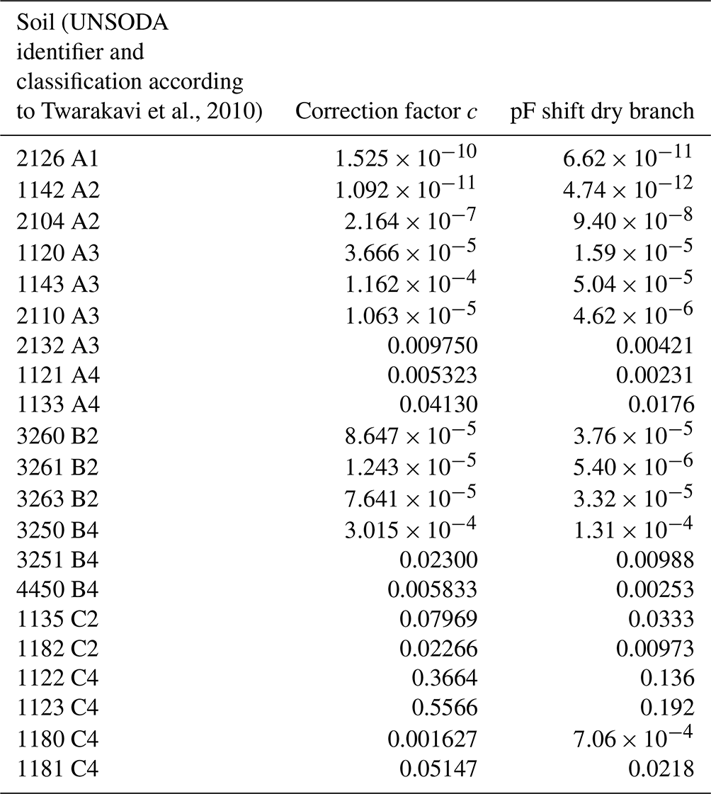
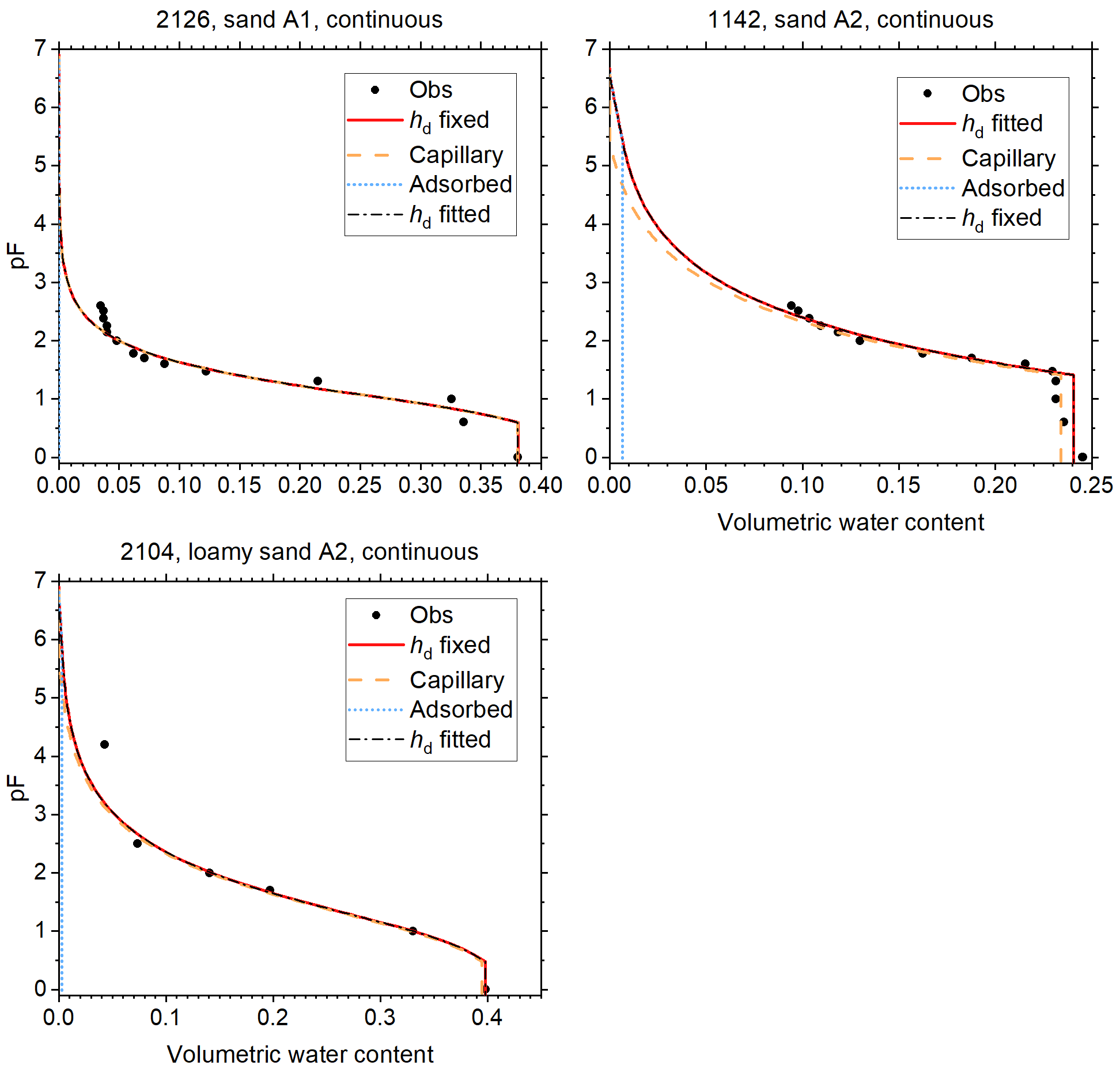
Figure 5Soil water retention data and fitted curves for soils of classes A1 and A2 of Twarakavi et al. (2010). Curves fitted with hd fixed at −106.8 cm H2O, and with hd fitted with a cap at that value are shown. The one with the lowest root mean square error is shown as a red solid line. The volume fractions of capillary-bound water and water adsorbed in films is shown for this curve. The other curve is shown as black dash–dot line. This curve has not been corrected for continuity at the junction point. The vertical axis denotes the logarithm (base 10) of the absolute value of the matric potential in cm H2O.
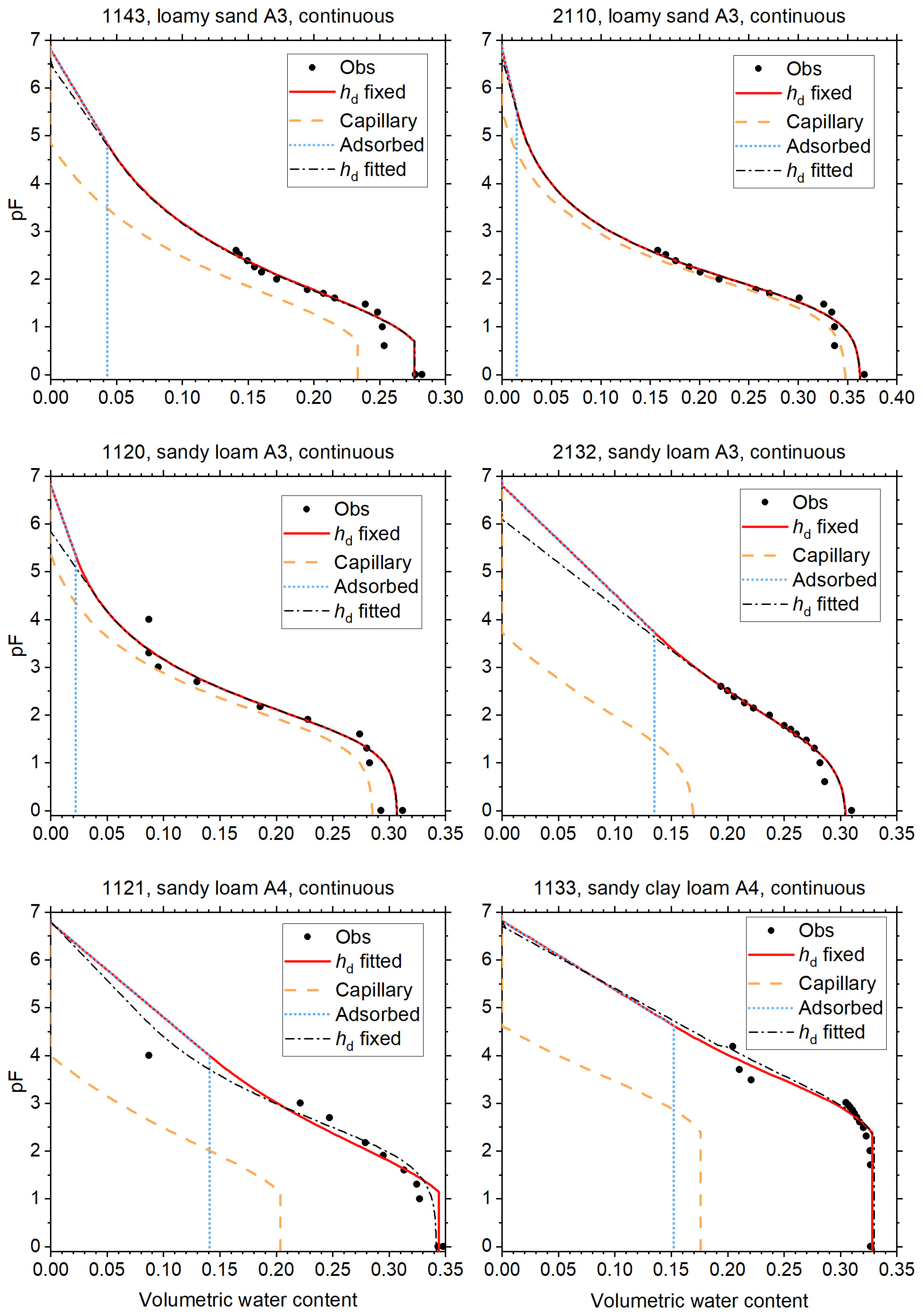
Figure 6As Fig. 5, for soils of classes A3 and A4 of Twarakavi et al. (2010).
The algorithm generates large numbers of sets of fitted parameter values. A random sample of these is used to determine the correlation matrix of the parameters. The best fit, its RMSE, and its correlation matrix are reported by the code for each of the three runs, and the run with the overall lowest RMSE is identified. The code returns a table of the fitted curve based on the best run, and reports the correction factor c used to compile this table. These tables are the basis for the plots shown below. If desired, the code also calculates the objective function on points of a regular grid covering the parameter space (map points) and writes a random sample of these to output. Even if this is not desired, a map is calculated based on a three point grid along each principal axis of the parameter space. This resulting output is helpful if a user wishes to verify if the objective function is correctly calculated.
Normally, the first complexes of each run are filled with randomly selected points in the valid regions of the parameter space. Optionally, only the complexes of run 3 are filled with randomly selected points, while the first complexes of run 1 are filled with the map points with the lowest RMSE. The first complexes of run 2 then contain these map points perturbed by adding random noise to the parameter values.
For each fitting parameter, a maximum and minimum value need to be provided. If these values are equal, the parameter is treated as a fixed value, and the dimensionality of the parameter space is reduced accordingly. The number of complexes is two (for eight of fewer fitting parameters) or four (see Duan et al., 1994). If this leads to frequent convergence at local minima, the number of complexes can be set to twice the number of fitting parameters. The number of individuals in a complex and the number of evolution steps are twice the number of fitting parameters plus one. The number of individuals in the subcomplexes is the number of fitting parameter plus one. The number of offspring in each evolution step is one. These settings are all in accordance with Duan et al. (1994).
When the user chooses to use the map of regularly spaced points in the parameter space to set the initial guesses of the first two runs, the code adapts the parameter ranges based on their ranges among the map points selected to fill the initial complexes.
The permitted parameter range for θs enveloped the range of observed saturated water contents, with a limited buffer on either side of the range. The range of hae was determined based on the wettest unsaturated data point and the driest saturated point, with a generous buffer. The range limit at the wet end was often set to zero. The value of hd was mostly fixed and occasionally varied over a relatively wide range depending on visual examination of the data points. The permitted range for α was 0.001 to 0.5, except for 1142, where alpha could go as high as 100.0. After some trial and error, the range of n was set relatively narrow (between 1.05 and 2) because even with wider ranges the fitted values fell within this range. Any time a fitted value was close to one of its limits, the fit was repeated with an expanded range.
No more than four convergence criteria were allowed to fail for convergence to be achieved. If convergence was not achieved, up to 20 000 evaluations of the objective function evaluations would be performed. The actual number could be slightly higher because it was checked each time a shuffle had been completed. A map was not created, and therefore all three optimization runs started with random parameter combinations filling the complexes. The maximum allowed relative change in the RMSE between consecutive shuffles was 10−6. The maximum allowed value of the RMSE was 0.1. For the parameters, the absolute tolerances for θs, hae, hd, α, and n were 0.001, 0.1, 1000.0, 0.1, and 0.01, respectively. The relative tolerances were 0.1 for α and 0.01 for the others. This choice reflects the limited sensitivity to α.
The internally set relative tolerances for parameter variations for all complexes combined and for the most successful complex were both 0.01. The internally set required maximum size of the hypercube enveloping the range of fitted parameter values (again for all complexes combined and the most successful one), scaled by the volume of the hypercube defined by the minimum and maximum allowed parameter values, equals 0.01d, with d the number of fitting parameters that were not set at fixed values by the user.
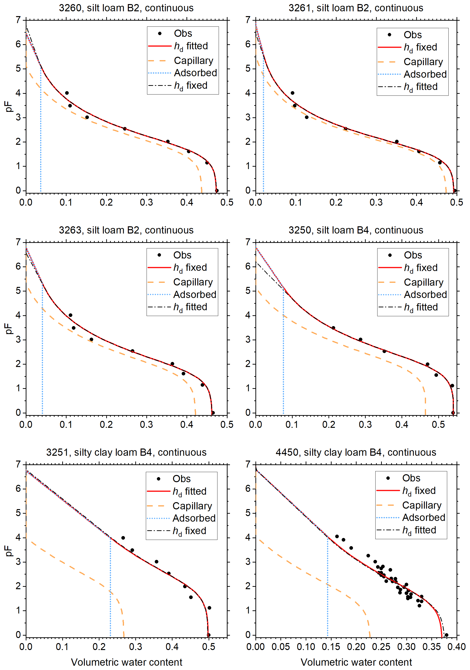
Figure 7As Fig. 5, for soils of classes B2 and B4 of Twarakavi et al. (2010).
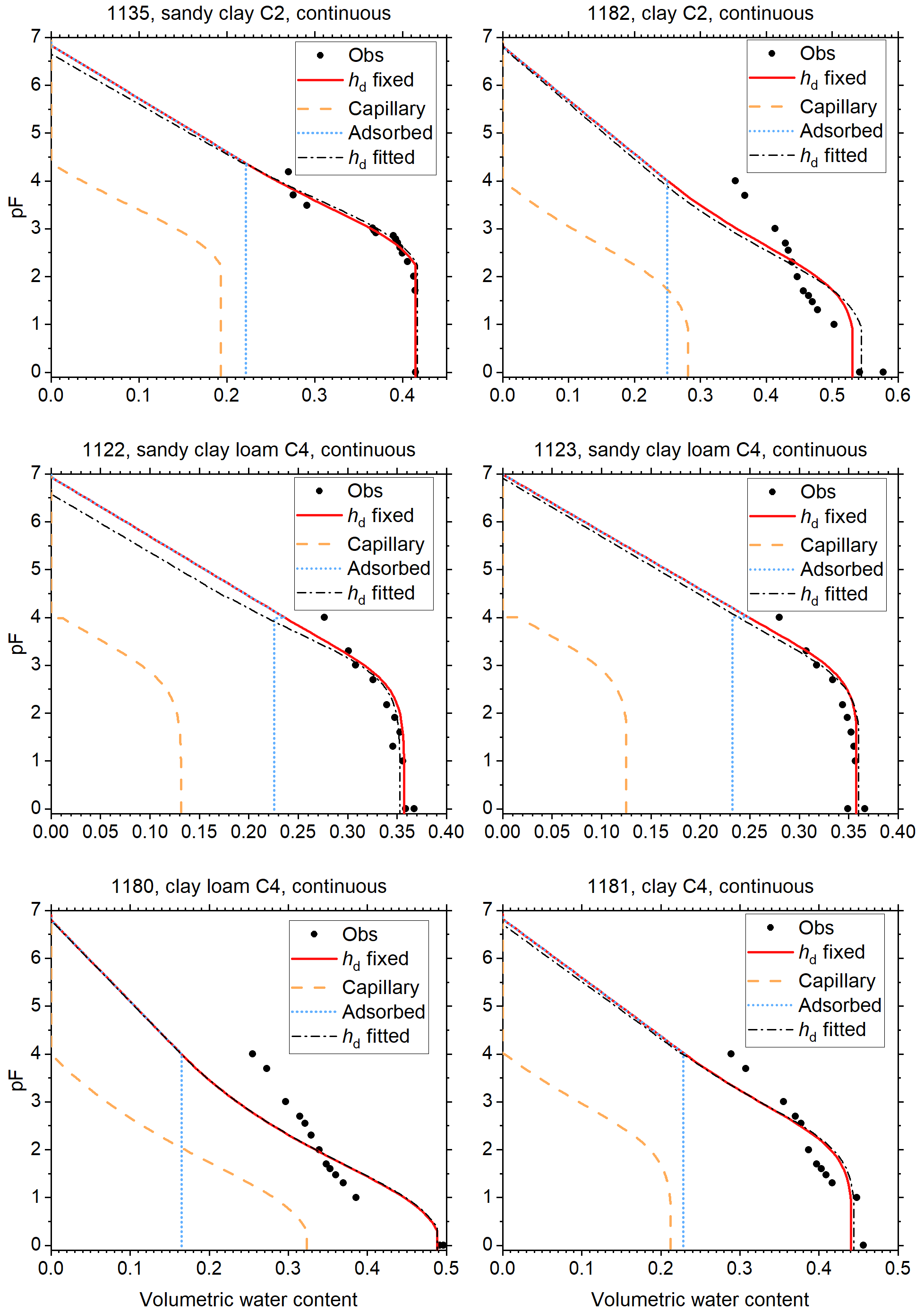
Figure 8As Fig. 5, for soils of classes C2 and C4 of Twarakavi et al. (2010).
In the tables that follow, the soil texture classification according to Twarakavi et al. (2010) is provided. The advantage of this classification over the conventional USDA soil texture classification is that it better recognizes differences in hydraulic behavior between its textural classes. This makes it more relevant for soil water flow studies for which the SWRCs are typically used.
Table 1 shows the fitted parameter values of the best fits, the resulting RMSE, and the corresponding value of hj. The value of α for soil 1142 stands out. As explained above, high values of α lead to a power-law type of SWRC between hae and hj. An additional fit with α capped at 1.0 confirmed that the shape of the SWRC is not very sensitive to large values of α. The increase in the RMSE caused by limiting the range of α was 10−4, and the changes in θs, hae, and n did not occur before the fourth significant digit. One can also switch from a sigmoidal model to a power-law model by invoking Eq. (9) if α is very large, keeping the fitted values of the other parameters.
Fuentes et al. (1991) showed that for values of n smaller than two, the asymptotic dry branch of the original parameterization of van Genuchten (1980) would lead to physically unacceptable behavior. All soils in Table 1 have values of n in this range. This highlights the importance of avoiding a dry branch with an asymptote at a residual water content.
The range of values of hj in Table 1 is only slightly beyond the range reported by Rossi and Nimmo (1994) for a smaller number of soils. This lends credibility to Eq. (8). In the few cases where hd was fitted, the resulting values in Table 1 are close to the value proposed by Schneider and Goss (2012). Table 2 shows the correction factor c of Eqs. (10) and (11), which ensures continuity of the SWRC. Seven of the 21 soils need a correction of hd that exceeds 1 %. The resulting shift of the dry-branch pF is also shown. For most soils, the shift is negligible. Only for soils 1122 and 1123 (both fine-textured soils with small values for both α and n), the shift exceeds 0.1 pF unit, but never more than 0.2 unit.
Only the optimizations for soils 1142 and 2104 converged, with convergence criteria 4, 6, 8, 9, and 10 satisfied for all parameters for soil 1142, and criteria 4 through 10 for soil 2104. None of the correlation coefficients of the parameter pairs for either soil exceeded 0.31. The other optimizations ran until the maximum number of objective function evaluations was exceeded. For soil 1120, criteria 9 and 10 were met for all parameters. For the remaining soils, criteria 1, 2, and 9 were satisfied in all cases. For 14 soils, criterion 10 was met as well. For soil 3250, criterion 8 was also satisfied. The lack of convergence forced the code to keep exploring the parameter space, leading to a large proportion of randomly selected points because the reflection and contraction points determined by the SCE algorithm did not improve the fit. If the majority of points is randomly selected, there is no correlation between the parameters, and the correlation matrix does not provide any information.
In all cases, the fitted parameter values for the runs with hd fixed and hd free and the three individual runs for each optimization were essentially in agreement, and the parameter values did not look suspect. Therefore, it was considered unnecessary to run the optimizations with modified convergence requirements in order to obtain more meaningful correlation matrices.
The reduced weights assigned to data points with pF>3 are reflected in the plots of Figs. 5 through 8, which show the fitted curves with hd fixed and hd fitted. In these plots, the fit with the lowest RMSE is plotted in red, and the corresponding curves for θc and θa are included. The other curve is shown in black. To illustrate how small the continuity correction c is, this curve is shown without this correction. The discontinuity at the junction point is only visible for soils 1133 (Fig. 6) and 1122 (Fig. 8).
The fraction of adsorbed water increases when moving from sands (Figs. 5 and 6) through loams (Figs. 6 and 7) to clays (Fig. 8). Because the separation between capillary and adsorbed water is abrupt and binary at hj, this should not be interpreted as representative for the more smooth transition in natural soils. Nevertheless, the direction of the trend is physically plausible.
Most soils (2126 and 1142 in Fig. 5; 1120, 1121, 1143, 2110, and 2132 in Fig. 6; 1142 and 2126 in Fig. 7; 1122, 1180, and 1182 in Fig. 8) have observed saturated water contents that seem to be too large compared to the other data points. The causes (e.g., macropores or air inclusion) are not known. Data points at saturation were assumed to be very accurate and therefore had a high weight, which the plots reflect. It sometimes results in relatively low (more negative) air-entry values in coarse soils (Figs. 5 and 6 and Table 1, most notably soil 1142).
All B2 soils (silt loams) and two out of three B4 soils (both silty clay loams) have high values of hae, indicating that the maximum pore size is large (Table 1). Although one would suspect that such fine-textured soils would have a low (more negative) air-entry value, the results are consistent with the data, as Fig. 7 shows. Some of the C2 and C4 soils (1180–1182) have high RMSE values (Table 1). Their plots in Fig. 8 reveal that the multimodal shape of the curves was not captured well by Eq. (1). The remaining soils in Fig. 8 had very few points in the dry range, and fixing hd was very effective in guiding the dry branch of the SWRC.
This paper focuses on mineral soils with unimodal SWRCs. If an extension to multimodality is desired, Eqs. (12)–(16) provide a starting point. Further testing on soils with specific characteristics, such as volcanic or organic soils, may be worthwhile. In the case of organic soils, the risk of irreversible changes will require some caution when measuring points on the SWRC.
The Fortran code for fitting the SWRC parameters and post-processing and its user manual are available from the Zenodo repository (https://doi.org/10.5281/zenodo.7271284, de Rooij, 2022).
The UNSODA database with the soil data can be downloaded at https://data.nal.usda.gov/dataset/unsoda-20-unsaturated-soil (Nemes et al., 2001).
The author is a member of the editorial board of Hydrology and Earth System Sciences. The peer-review process was guided by an independent editor, and the author also has no other competing interests to declare.
Publisher’s note: Copernicus Publications remains neutral with regard to jurisdictional claims in published maps and institutional affiliations.
I thank the reviewers for their constructive comments.
The article processing charges for this open-access publication were covered by the Helmholtz Centre for Environmental Research – UFZ.
This paper was edited by Bob Su and reviewed by five anonymous referees.
Assouline, S. and Or, D.: Conceptual and parametric representation of soil hydraulic properties: a review, Vadose Zone J., 12, 1–20, https://doi.org/10.2136/vzj2013.07.0121, 2013.
Bittelli, M. and Flury, M.: Errors in water retention curves determined with pressure plates, Soil Sci. Soc. Am. J., 73, 1453–1460, https://doi.org/10.2136/sssaj2008.0082, 2009.
Brooks, R. H. and Corey, A. T.: Hydraulic properties of porous media, Colorado State University, Hydrology Paper No. 3, 27 pp., 1964.
Davis, J. L. and Annan, A. P.: Ground penetrating radar to measure soil water content, in: Methods of soil analysis. Part 4 – Physical methods, edited by: Dane, J. H. and Topp, G. C., Soil Science Society of America, Inc., Madison, Wisconsin, USA, https://doi.org/10.2136/sssabookser5.4, 446–463, 2002.
Dettmann, U., SoilHyp: Soil Hydraulic Properties, https://rdrr.io/cran/SoilHyP/ (last access: 1 April 2022), 2021.
de Rooij, G.: Fitting the parameters of the RIA parameterization of the soil water retention curve (1.1), Zenodo [code], https://doi.org/10.5281/zenodo.7271284, 2022.
de Rooij, G. H., Mai, J., and Madi, R.: Sigmoidal water retention function with improved behaviour in dry and wet soils, Hydrol. Earth Syst. Sci., 25, 983–1007, https://doi.org/10.5194/hess-25-983-2021, 2021.
Du, C.: Comparison of the performance of 22 models describing soil water retention curves from saturation to oven dryness, Vadose Zone J., 19, e20072, https://doi.org/10.1002/vzj2.20072, 2020.
Duan, Q. Y., Gupta, V. K., and Sorooshian, S.: Shuffled complex evolution approach for effective and efficient global minimization, J. Opti. Theory Appl., 76, 501–521, 1993.
Duan, Q., Sorooshian, S., and Gupta, V.: Effective and efficient global optimization for conceptual rainfall–runoff models, Water Resour. Res., 28, 1015–1031, 1992.
Duan, Q., Sorooshian, S., and Gupta, V.: Optimal use of the SCE–UA global optimization method for calibrating watershed models, J. Hydrol., 158, 265–284, 1994.
Durner, W.: Hydraulic conductivity estimation for soils with heterogeneous pore structure, Water Resour. Res., 30, 211–223, 1994.
Ferré, P. A. and Topp, G. C.: Time domain reflectometry, in: Methods of soil analysis. Part 4 – Physical methods, edited by: Dane, J. H. and Topp, G. C., Soil Science Society of America, Inc., Madison, Wisconsin, USA, 434–446, https://doi.org/10.2136/sssabookser5.4, 2002.
Fuentes, C., Haverkamp, R., Parlange, J.-Y., Brutsaert, W., Zayani, K., and Vachaud, G.: Constraints on parameters in three soil–water capillary retention functions, Trans. Porous Media, 6, 445–449, 1991.
Ippisch, O., Vogel, H.-J., and Bastian, P.: Validity limits for the van Genuchten–Mualem model and implications for parameter estimation and numerical simulation, Adv. Water Resour., 29, 1780–1789, https://doi.org/10.1016/j.advwatres.2005.12.011, 2006.
Lawrence, D. M., Fisher, R. A., Koven, C. D., Oleson, K. W., Swenson, S. C., Bonan, G., Collier, N., Ghimire, B., van Kampenhout, L., Kennedy, D., Kluzek, E., Lawrence, P. J., Li, F., Li, H., Lombardozzi, D., Riley, W. J., Sacks, W. J., Shi, M., Vertenstein, M., Wieder, W. R., Xu, C., Ali, A. A., Badger, A. M., Bisht, G., van den Broeke, M., Brunke, M. A., Burns, S. P., Buzan, J., Clark, M., Craig, A., Dahlin, K., Drewniak, B., Fisher, J. B., Flanner, M., Fox, A. M., Gentine, P., Hoffman, F., Keppel-Aleks, G., Knox, R., Kumar, S., Lenaerts, J., Leung, L. R., Lipscomb, W. H., Lu, Y., Pandey, A., Pelletier, J. D., Perket, J., Randerson, J. T., Ricciuto, D. M., Sanderson, B. M., Slater, A., Subin, Z. M., Tang, J., Thomas, R. Q., Val Martin, M., and Zeng, X.: The Community Land Model version 5: Description of new features, benchmarking, and impact of forcing uncertainty, J. Adv. Model. Earth Syst., 11, 4245–4287, https://doi.org/10.1029/2018MS001583, 2019.
Madi, R., de Rooij, G. H., Mielenz, H., and Mai, J.: Parametric soil water retention models: a critical evaluation of expressions for the full moisture range, Hydrol. Earth Syst. Sci., 22, 1193–1219, https://doi.org/10.5194/hess-22-1193-2018, 2018.
National Agricultural Library: UNSODA Database, USDA [data set], https://data.nal.usda.gov/dataset/unsoda-20-unsaturated-soil (last access: 22 July 2020), 2015.
Nemes, A., Schaap, M. G., Leij, F. J., and Wösten, J. H. M.: Description of the unsaturated soil hydraulic database UNSODA version 2.0, J. Hydrol., 251, 152–162, https://doi.org/10.1016/S0022-1694(01)00465-6, 2001.
Or, D. and Tuller, M.: Liquid retention and interfacial area in variably saturated porous media: Upscaling from single–pore to sample–scale model, Water Resour. Res., 35, 3591–3605, 1999.
Rossi, C., and Nimmo, J. R.: Modeling of soil water retention from saturation to oven dryness, Water Resour. Res., 30, 701–708, 1994.
Schneider, M. and Goss, K.-U.: Prediction of the water sorption term in air dry soils, Geoderma, 170, 64–69, https://doi.org/10.1016/j.geoderma.2011.10.008, 2012.
Šimůnek, J., van Genuchten, M. Th., and Šejna, M.: Recent developments and applications of the HYDRUS computer software packages, Vadose Zone J., 15, 1–25, https://doi.org/10.2136/vzj2016.04.0033, 2016.
Solone, R., Bittelli, M., Tomei, F., and Morari, F.: Errors in water retention curves determined with pressure plates: Effects on the soil water balance, J. Hydrol., 470–471, 65–74, https://doi.org/10.1016/j.jhydrol.2012.08.017, 2012.
SWAP Soil Water Atmosphere Plant, https://www.swap.alterra.nl/, last access: 10 August 2022.
Tuller, M. and Or, D.: Water films and scaling of soil characteristic curves at low water contents, Water Resour. Res., 41, W09403, https://doi.org/10.1029/2005WR004142, 2005.
Twarakavi, N. K. C., Šimůnek, J., and Schaap, M. G.: Can texture–based classification optimally classify soils with respect to soil hydraulics?, Water Resour. Res., 46, W01501, https://doi.org/10.1029/2009WR007939, 2010.
van Genuchten, M. Th.: A closed–form equation for predicting the hydraulic conductivity for unsaturated soils, Soil Sci. Soc. Am. J., 44, 892–898, 1980.
Wang, Y., Ma, R., and Zhu, G.: Improved prediction of hydraulic conductivity with a soil water retention curve that accounts for both capillary and adsorption forces, Water Resour. Res., 58, e2021WR031297, https://doi.org/10.1029/2021WR031297, 2022.