the Creative Commons Attribution 4.0 License.
the Creative Commons Attribution 4.0 License.
 | 17 Nov 2022
How can we benefit from regime information to make more effective use of long short-term memory (LSTM) runoff models?
Reyhaneh Hashemi
Pierre Brigode
Pierre-André Garambois
Pierre Javelle
To date, long short-term memory (LSTM) networks have been successfully applied to a key problem in hydrology: the prediction of runoff. Unlike traditional conceptual models, LSTM models are built on concepts that avoid the need for our knowledge of hydrology to be formally encoded into the model. The question, then, is how we can still make use of our domain knowledge and traditional practices, not to build the LSTM models themselves, as we do for conceptual models, but to use them more effectively. In the present paper, we adopt this approach, investigating how we can use information concerning the hydrologic characteristics of catchments for LSTM runoff models. In this first application of LSTM in a French context, we use 361 gauged catchments with very diverse hydrologic conditions from across France. The catchments have long time series of at least 30 years. Our main directions for investigation include (a) the relationship between LSTM performance and the length of the LSTM input sequence within different hydrologic regimes, (b) the importance of the hydrologic homogeneity of catchments when training LSTMs on a group of catchments, and (c) the interconnected influence of the local tuning of the two important LSTM hyperparameters, namely the length of the input sequence and the hidden unit size, on the performance of group-trained LSTMs. We present a classification built on three indices taken from the runoff, precipitation, and temperature regimes. We use this classification as our measure of homogeneity: catchments within the same regime are assumed to be hydrologically homogeneous. We train LSTMs on individual catchments (local-level training), on catchments within the same regime (regime-level training), and on the entire sample (national-level training). We benchmark local LSTMs using the GR4J conceptual model, which is able to represent the water gains/losses in a catchment. We show that LSTM performance has the highest sensitivity to the length of the input sequence in the Uniform and Nival regimes, where the dominant hydrologic process of the regime has clear long-term dynamics; thus, long input sequences should be chosen in these cases. In other regimes, this level of sensitivity is not found. Moreover, in some regimes, almost no sensitivity is observed. Therefore, the size of the input sequence in these regimes does not need to be large. Overall, our homogeneous regime-level training slightly outperforms our heterogeneous national-level training. This shows that the same level of data adequacy with respect to the complexity of representation(s) to be learned is achieved in both levels of training. We do not, however, exclude a potential role of the regime-informed property of our national LSTMs, which use previous classification variables as static attributes. Last but not least, we demonstrate that the local selection of the two important LSTM hyperparameters (the length of the input sequence and the hidden unit size) combined with national-level training can lead to the best runoff prediction performance.
- Article
(6522 KB) - Full-text XML
- BibTeX
- EndNote


Surface-water runoff (referred to hereafter as runoff) is the response of a catchment to its intakes and yields. The reliable prediction of runoff is essential for the management of many water-related hazards and water resources, and it has been the focus of numerous studies in hydrology over the past decades. Nevertheless, the accurate prediction of runoff has remained a challenge due to the non-linearity of the several surface and subsurface processes involved (Kachroo and Natale, 1992; Phillips, 2003). Promising continuous runoff models based on long short-term memory (LSTM) (Hochreiter and Schmidhuber, 1997) were first introduced by Kratzert et al. in 2018. This highly successful first application has since encouraged many researchers to more widely explore the predictive capability of LSTM-based runoff models. Examples include Kratzert et al. (2019a, b), Gao et al. (2020), O et al. (2020), Feng et al. (2020), Frame et al. (2021), Gauch et al. (2021a, b), Lees et al. (2021), and Nearing et al. (2021). Unlike traditional conceptual rainfall–runoff models, where hydrological rules are hardwired into the model, LSTM-based models borrow their principles from fields that are not traditionally associated with hydrology. Thus, a central interest is whether and how we can benefit from domain knowledge and traditional practices in hydrology when using LSTM models for the prediction of runoff. This paper considers some pathways towards this goal.
Path 1
Conforming to the daily runoff model from Kratzert et al. (2018), the LSTM takes a “sequence” of past forcing variables to predict runoff. Its sequence-type input reflects the distinctive property of LSTMs: capturing time dependencies. In the previous studies by Kratzert et al. (2018) and Lees et al. (2021), the length of this sequence, hereafter called “lookback”, was set to 365 d so that the dynamics of a full annual cycle could be captured. Kratzert et al. (2019b) tested four lookbacks (90, 180, 270, and 365 d) and reported that a lookback of 270 d gave the best results in their study. However, Gauch et al. (2021b) systematically reduced the size of the data and showed that the choice of lookback should consider the amount of data: when the available data were limited, an overly long lookback could impair LSTM performance. From the point of view of pure deep learning, lookback is a hyperparameter of the same type as batch size, learning rate, and so forth. However, there are some compelling reasons to separate lookback from the usual hyperparameters. The catchment response is known to depend on the current soil moisture state of the catchment, which is itself a result of antecedent conditions and forcing history, for example, a succession of dry/wet, cold/hot periods. However, this dependence is time limited; thus, what has happened in the past is progressively forgotten by the catchment and, over time, it will have no (or very limited) influence on current conditions. It is also known that each catchment has its own memory length, which is related to the time taken by the catchment to dissipate the input information. For instance, large catchments connected to major aquifers can have a long memory of up to several years (de Lavenne et al., 2021). By contrast, small catchments located on the surface of an impermeable bedrock with no infiltration can have a very short memory of only a few days. Hence, we expect the choice of lookback to depend not only on the length of training data, as shown by Gauch et al. (2021b), but also on the hydrologic characteristics of the catchment. Thus, we can define our first research question (Q1), which is largely unaddressed in the existing literature, as follows: “Does the LSTM performance–lookback pattern depend on the catchment regime?”.
Deep learning context for paths 2 and 3
We can decompose the error associated with any deep learning network (including LSTM) to the following three components (Beck et al., 2022): (1) approximation error, (2) generalization error, and (3) optimization error. The approximation error is the error of the network in approximating the true underlying mapping function. This error is controlled by model representational capacity (which depends itself on the model architecture and neural network family, for example, vanilla multilayer perceptron, LSTM, or convolutional neural networks) as well as by the choice and number of input features (Goodfellow et al., 2016). The generalization error is the error of the network on unseen data. The optimization error is the error of the optimization algorithm in finding the global minimum of the loss function. This error results from the optimization algorithm. The training and validation errors that the learning algorithm encounters during training reflect the approximation plus optimization and generalization errors respectively. However, the training and validation errors are only “expectations” or “estimates” of the true errors, as they are computed on only “a finite number” of samples drawn from the distribution of inputs that the system is expected to encounter in practice (Goodfellow et al., 2016). As the number of training examples increases, the network's learning can be refined given the more accurate losses and the larger number of gradient updates. We may, therefore, plausibly treat data size as a model-independent factor controlling the performance of the model. Here, we assume that the model family and architecture as well as the optimization algorithm are predetermined, and, thus, that all errors associated with them remain unchanged. In this paper, we set out to alter other error-controlling variables (i.e. features of the model, data size, and data homogeneity) – in ways that conform to traditional hydrologic practices – and study how LSTM performance changes. Path 2 allows for the investigation of the influence of the model's features and data size. Through path 3, we observe the influence of data homogeneity.
Path 2
In line with classical regionalization (Kratzert et al., 2018, 2019b), we move from individually trained (local) to group-trained (regional) LSTMs. In doing so, we also incorporate static features (into regional LSTMs), increasing both data size and model capacity. Bigger data and higher capacity improve the training error and model precision, but can they can do so without losing some generalization? This path allows us to formulate our second question (Q2): “To what degree does the LSTM trade generalization for precision in moving from local to regional training?”.
Local and regional LSTMs have already been investigated and compared against multiple conceptual models in several studies. The reader is referred to Kratzert et al. (2018) for comparison of local LSTMs with the Sacramento Soil Moisture Accounting Model (SAC-SMA; Burnash et al., 1973) coupled with the Snow-17 conceptual model. For examples of regional LSTMs, the reader is referred to Kratzert et al. (2019b) or to Lees et al. (2021) and Gauch et al. (2021a). Kratzert et al. (2018) suggest that, in regional training, not only are the training data significantly augmented but inclusion of different contributing catchments would also introduce further complementary information about rainfall–runoff transformation under more general hydrological conditions and, consequently, learning would improve. Kratzert et al. (2019a, b) demonstrated that their regional LSTMs using both dynamic (e.g. forcing data) and static (e.g. catchment attributes) features outperformed the regional LSTMs with no static features as well as outperforming all local conceptual benchmark models tested. Subsequently, Lees et al. (2021) also reported that regional LSTM models outperformed their four conceptual benchmark models in the climatic context of Great Britain and on a sample of 518 catchments. However, none of the previous studies compared local LSTMs to regional LSTMs with static attributes.
Path 3
Seeking to benefit from traditional methods of hydrologic classification (Haines et al., 1988; Oudin et al., 2008; Chiverton et al., 2015), we investigate hydrologically homogeneous versus hydrologically heterogeneous training at the regional scale in this work. Classification of catchments according to their hydrologic behaviour conveys the idea that all catchments in the same class are hydrologically similar to each other and, thus, have the same behaviour or the same “representation” in the language of deep learning. But, may it also be advantageous to LSTM learning, allowing the regional LSTMs to capture the shared behaviour using a single training session on the data for the class? This is the main focus of this path where we compare regional LSTMs under two conditions: (a) when the training examples are greater in number but collected from distributions that are very different with respect to their hydrologic statistics (heterogeneous national training set) and (b) when there are far fewer training examples but these are drawn from hydrologically similar distributions (homogeneous regime training set). In this comparison, the model capacity/complexity remains the same, the size of the training data increases, and the complexity of the latent rules to be learned varies due to the difference in heterogeneity/homogeneity. More specifically, we are interested in answering the following question (Q3): “Is there a performance gain for regional LSTMs in the shift from hydrologically heterogeneous to homogeneous training and vice versa?”.
To identify hydrologic similarity, we present a purely hydrologic classification built on three indices obtained from the analysis of runoff, precipitation, and temperature regimes. To date, only one other investigation of the data homogeneity component in training LSTMs has been undertaken in a recently published study conducted in parallel with the present research (Fang et al., 2022). However, there are a number of important differences between the present paper and the study by Fang et al. (2022). Their study is conducted within the US context. They use the “ecoregion-based” classification of Omernik and Griffith (2014), which is built on geological, land-form, soil, vegetation, climatic, land-use, wildlife, and hydrologic compositions (Fang et al., 2022). The measure of homogeneity that is used in their experimental design is the “proximity” of ecoregions: the further apart the two regions are, the more dissimilar they are. However, this hypothesis has not always been found to be true, as is shown in Oudin et al. (2008). Likewise, this hypothesis is largely contradicted in our classification, which allows very close but also totally dissimilar catchments and vice versa. Not only is their LSTM model different in many respects (e.g. a different architecture, number of hidden layers, activation function, and loss function), Fang et al. (2022) have performed no hyperparameter tuning for lookback (it is fixed at 365 d). Furthermore, the number of epochs used in their study is predefined and similar for all experiments, which is not the case in the present paper.
Path 4
The last investigation path in this paper – inspired by the fine-tuning experiment performed by Kratzert et al. (2018) – is about improving LSTM performance by a method other than increasing the size of the data/model capacity or changing the homogeneity/heterogeneity of the data. Here, we study the influence of the approach to the selection of two major LSTM hyperparameters: lookback and hidden unit size. Following this path, our last research question (Q4) is defined as follows: “What is the most effective way of using LSTMs to predict runoff?”.
In pursuing these paths, we apply LSTM to a sample consisting of 361 gauged catchments with very diverse hydrologic conditions from all over France; this paper is the first application of LSTM to the French context. The discharge time series of the catchments is at least 30 years in length (between 30 and 60 years). In all experiments, the LSTM is tuned with respect to the lookback and hidden unit size as well as the dropout rate, and three disjoint subsets (training, validation, and test) are used. We also use the non-mass-conservative GR4J conceptual model to benchmark the LSTM.
The remainder of this paper is organized as follows. The next section presents the available data and our hydrologic catchment classification. Section 3 details the methods used in this paper and describes the experimental design. Results are provided in Sect. 4. The paper's research questions are discussed in Sect. 5. The conclusion is found in Sect. 6, which also outlines some future directions based on the findings of this study.
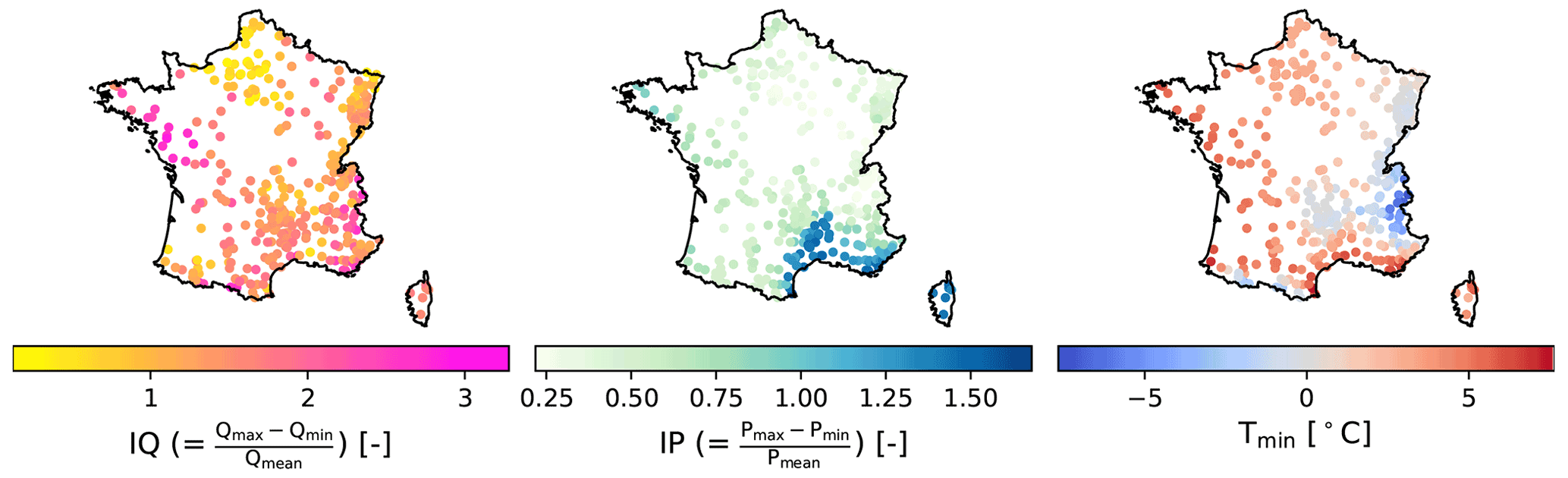
Figure 1Spatial variation in the three indices used for hydrologic catchment classification: IQ, IP, and Tmin. Each catchment in the sample is shown as a point.
2.1 Hydrometeorological data
The data set used in this study contains time series of hydrometeorological variables and time-invariant catchment attributes. It is a subset of a larger data set of 4190 French catchments (Delaigue et al., 2020). The meteorological forcing data are taken from the daily SAFRAN (Système d'Analyse Fournissant des Renseignements Atmosphériques à la Neige) reanalysis run by Météo France at a resolution of 8 km × 8 km (Quintana-Segui et al., 2008; Vidal et al., 2010). For each catchment, spatially averaged forcing data consisting of daily total precipitation; mean, minimum, and maximum air temperature; wind speed; air moisture; atmospheric radiation; and visible radiation are available for a common period from 1 August 1958 to 31 July 2019. Hydrometric data consist of daily discharge time series covering the period of the forcing data.
The catchment sample for this paper includes 361 catchments from all over France with discharge time series ranging from 30 to 60 years. These catchments range in size from 5 to 13 806 km2 with a median size of 219 km2. Their annual runoff ranges from 47 to 2312 mm yr−1, with a median value of 466 mm yr−1, and annual total precipitation varies between 621 and 2128 mm yr−1, with a median value of 1053 mm yr−1. The mean daily temperature of the catchments varies between −1.8 and 14.8 ∘C and has a median value of 9.8 ∘C.
2.2 Catchment classification
The classification proposed in this paper uses readily available data and is inspired by Pardé (1933) and Sauquet (2006). It is built on three hydroclimatic indices, namely IQ (–), IP (–), and Tmin (∘C), derived from the analysis of interannual monthly runoff (Q, mm per month), total precipitation (P, mm per month), and temperature (T, ∘C) signals. These indices are defined as follows:
Here, Ti is the mean annual temperature of month i, Qmax and Qmin are maximum and minimum interannual monthly runoff (mm per month) respectively, and Pmax and Pmin are maximum and minimum interannual monthly total precipitation (mm per month) respectively.
In this definition, the IQ and IP indices give information on runoff variability and precipitation variability throughout the year respectively. Low values for IQ and IP indicate their uniform distribution across the year, whereas a high value reflects the presence of contrasting dry and wet seasons. A low IQ can also imply the presence of groundwater or reservoirs (natural or artificial), which tend to attenuate runoff fluctuations at the catchment outlet. The Tmin index is a proxy to determine whether or not precipitation falls as snow during winter. Figure 1 shows the spatial variation in the three indices across France. High IQ levels are fragmented in patches in the west and south-east of the country. The areas with high IP levels are found on the Mediterranean coast in the south and on Corsica. Low Tmin values occur in the mountainous areas: the Alps in the east, the Pyrenees in the south-west, and the Massif Central in the centre of France.
Using the specified indices, the following classification criteria are defined and applied to each catchment in the sample to determine its hydrologic regime (Fig. 2):
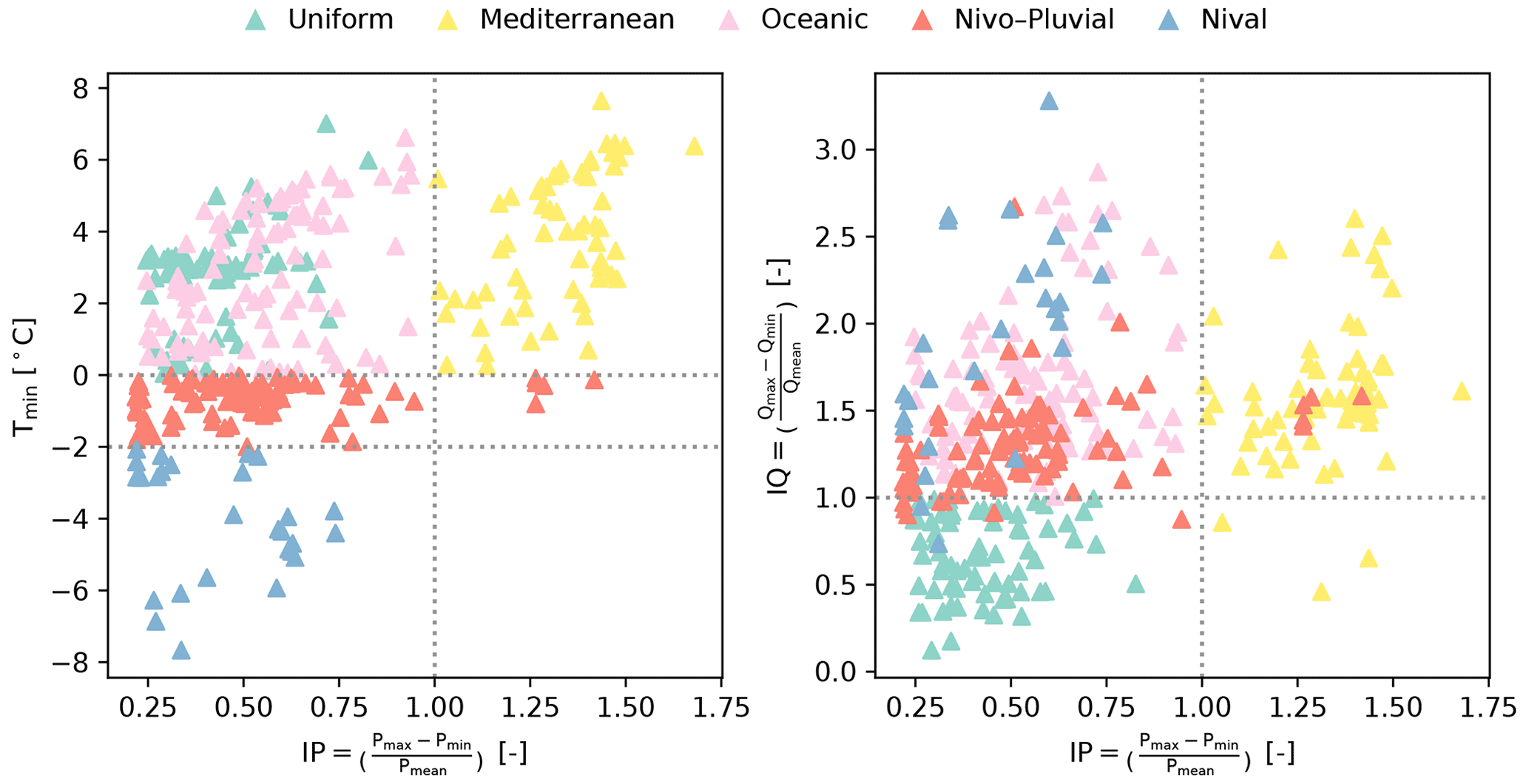
Figure 2Classification of the catchments into five hydrologic regimes based on five conditions built on Tmin, IP, and IQ. In order of priority, we first evaluate two Tmin conditions: and . For catchments not satisfying either of these two conditions, we then check if IP>1. If this condition is also unsatisfied, the IQ>1 condition is evaluated. Each point represents a catchment, and its colour indicates its regime.
The location of the catchments within each regime is shown in Fig. 3. We can observe that the regimes are geographically plausible and compatible with the geographical characteristics of the region. For example, the Nival and Nivo–Pluvial regimes occur in the mountainous ranges, and the catchments with a Mediterranean regime are found along the French Mediterranean coastline and on the Mediterranean island of Corsica. The Oceanic catchments are distributed across other parts of France, except in areas known to have large aquifers belonging to the Uniform regime (e.g. the Paris Basin region in the north of France).
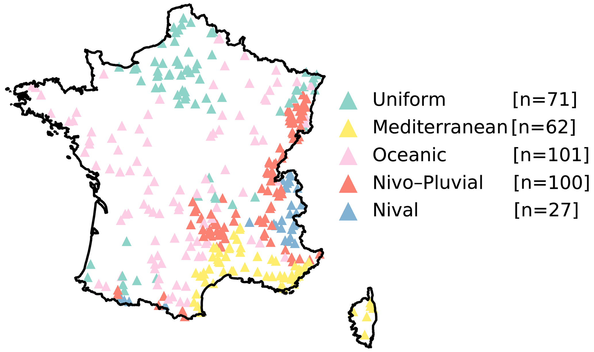
Figure 3Distribution of catchments from each of the five regimes across France: Uniform, Mediterranean, Oceanic, Nivo–Pluvial, and Nival. Each point represents one catchment and is coloured according to its regime.
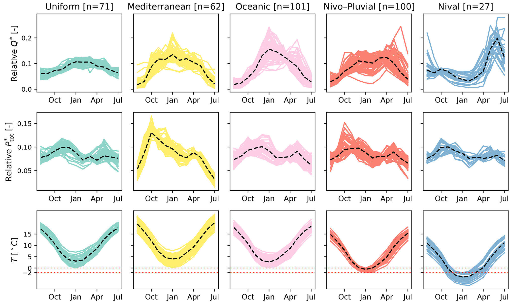
Figure 4Interannual monthly (or regime of) runoff (Q∗) (–), total precipitation () (–), and temperature (T) (∘C) for the catchments within different hydrologic regimes. The (∗) symbol in Q∗ and indicates that values for these two variables are relative to the total annual amount. Each solid line represents one catchment. The black dashed line in each panel represents the panel's median regime.
For each regime, variations in interannual monthly runoff, total precipitation, and mean temperature are presented in Fig. 4. In the Uniform regime, runoff remains in the range between 4 % and 13 % of annual discharge throughout the year, and no wet or dry period is observed. Meanwhile, the other regimes clearly exhibit periods of low and high flows. The Oceanic regime is characterized by low flows during the summer and high flows during the winter. This is due to higher evaporation in summer relative to winter. Total precipitation displays a rather uniform pattern in this regime. For catchments in the Mediterranean regime, high flows extend across a longer period but are less pronounced compared with the Oceanic regime. However, low flows occur at lower levels as a result of the extremely dry summers. Autumn precipitation is abundant in this regime, making autumn a period prone to thunderstorms which could, in turn, induce sudden flash floods. The runoff pattern in the Nival class is also recognizable with its snowmelt-induced peak in the late spring/early summer once the temperature rises. The Nivo–Pluvial regime appears to be a combination of the Oceanic and Nival regimes, with two high-flow periods, in autumn and spring.
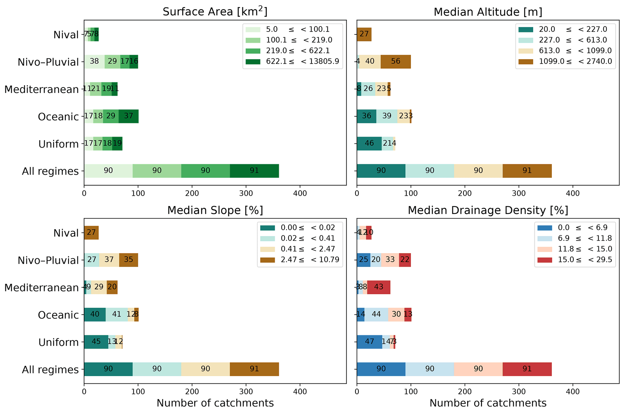
Figure 5Stacked bar charts showing the variation in the four physical attributes used in this paper within each regime and the entire sample. The end-to-end segments of each bar correspond to the intervals for each quartile of the physical attribute of interest. The quartiles are computed by taking all 361 catchments into account. The number inside each segment denotes its length.
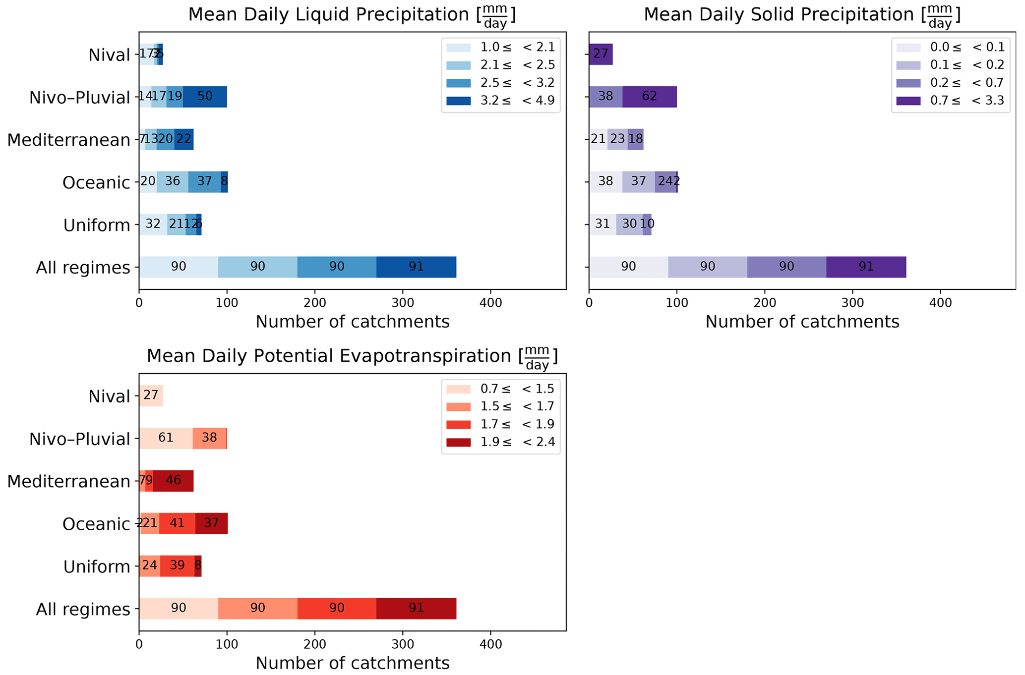
Figure 6Stacked bar charts showing the variation in the three climatic attributes used in this paper within each regime and the entire sample. The end-to-end segments of each bar correspond to the intervals for each quartile of the climatic attribute of interest. The quartiles are computed by taking all 361 catchments into account. The number inside each segment denotes its length.
2.3 Physical and climatic catchment attributes
In this paper, we use four physical attributes – surface area (km2), median slope (%), median drainage density (%), and median altitude (m) – as well as six climatic attributes – IP, IQ, Tmin, mean daily liquid precipitation (Pliq) (mm d−1), mean daily solid precipitation (Psol) (mm d−1), and mean daily potential evapotranspiration (PET) (mm d−1). The quartile distribution of the physical attributes and Pliq, Psol, and PET is shown in Figs. 5 and 6. We note that surface areas in all regimes are distributed across the four quartiles. That is, all regimes have catchments from almost all four quartiles. This is not, however, the case for other attributes. For example, catchments with the highest 25 % of values for altitude or slope are more likely to belong to the Nival or Nivo–Pluvial regimes. Similarly, it is more probable that catchments with the lowest 25 % of drainage densities will belong to the Uniform regime than to the Nival or Mediterranean regimes. In accordance with the features of the regime, Nival catchments have significant snow days, Nivo–Pluvial catchments have both major snow and rain days, and Mediterranean catchments have high evapotranspiration and rainfall rates.
3.1 A primer in long short-term memory (LSTM)
LSTM networks are a family of recurrent neural networks (RNNs) that address issues of both vanishing and exploding gradients (Hochreiter, 1998). They have proven well suited to the modelling of a time-dependent system where there can be “unknown lags” in a system's response to a continuous input. This is the case for the transformation of rainfall into runoff in a catchment. In the language of LSTM, the capture of time dependencies can be translated as sharing important information between time steps of a time sequence (Goodfellow et al., 2016). Information sharing in RNNs is supposed to be deep – i.e. between time steps that are distant from each other. However, in practice, this occurs only at a shallow level due to the vanishing gradient problem. The LSTM is designed, in turn, to allow for both shallow and deep information sharing across a sequence. In the following paragraphs, we provide a brief reminder of the forward propagation equations of a standard LSTM cell for time step t. For a comprehensive description of LSTM networks, we refer the reader to Chapter 10 of Goodfellow et al. (2016). Equations (4) to (9) given below are all from Goodfellow et al. (2016), with a slightly different notation. Figure 7 illustrates an unfolded computational LSTM cell corresponding to the last time step (t) of a sequence of length T (hence including time steps to t). This sequence reflects one sample in a (mini)batch.
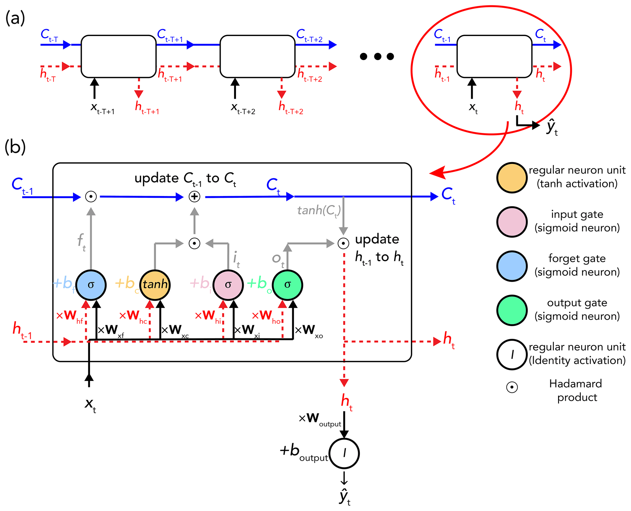
Figure 7(a) Time-unfolded schematic representation of data processing for a single sample consisting of T time steps – from time step to time step t. (b) Data processing of the last time step of the above sample through an LSTM cell. xt is the input of time step t, ht is the hidden state (dashed red line), Ct represents the cell state (solid blue line), and σ and tanh are the respective sigmoid and hyperbolic tangent functions. The figure is adapted from Olah (2015).
The standard LSTM involves two feedback connections operating at different timescales: the shallow-level hidden state (ht), for capturing short-term dependency details, and the deep-level cell state (Ct), for transferring information from the distant past to the present in a more effective way than the hidden state thanks to its “self-loop” structure. The equation of this self-loop is the core equation of the LSTM and is as follows:
It describes the cell state as a linear self-loop of form , with A:=ft and . ft, defined as
is called the forget gate and has the following properties:
-
It is a unit analogous to a neuron in nature, meaning that (1) it takes a weighted sum of its inputs (x,h) and a vector of bias (b), and (2) like an activation function, it applies an element-wise non-linearity to their sum.
-
Its non-linear function is the sigmoid function (σ) and has output values between 0 and 1 – . Its “gate” functionality derives from this property. A value of 0 tells the cell to completely disregard information, whereas a value of 1 tells it to fully retain information.
-
The presence of the term Wxt reflects a conditioning on the inputs of the current time step (xt). Therefore, ft is a function of xt and is different for different time steps. The weights W and bias b are independent of the inputs and are shared between different time steps.
ht−1 in Eq. (5) is the hidden state of the previous time step (t−1) and is defined as follows:
where ot is called the output gate. ot has the following definition:
and has exactly the same properties as ft.
So far, we have provided the definition of all terms in Eq. (4), except for it. It is called the input gate and is given by
Like the other gates and as Eq. (8) suggests, it shares all of the properties mentioned above for ft.
The network output at time step t () is computed by a regular neuron unit using the hidden state at time step t (ht) as input:
It is now clear that ht itself depends on the T last hidden states.
The notation, dimensions (for a single time step), and definition of the different variables in the LSTM's forward pass equations are given in Table 1.
3.2 Training, validation, and test data sets
The period for which there is a full discharge record differs between the catchments in the sample. To obtain training, validation, and test data sets, the data for each individual catchment are divided into three sets as follows: the most recent period containing 10 years of full discharge records is set as the test period; working backwards, the next period that contains 10 years of full discharge records is set as the validation period; and what remains constitutes the training period, the length of which varies between 10 and 40 years in the sample.
As the values for features and the target vary widely, a feature-wise standardization for the features and the target is performed. The standardization is performed using the mean and the standard deviation of the training data. This form of standardization – where the input data are centred around 0 and are scaled by the standard deviation – is also used by Kratzert et al. (2018) and is appropriate for runoff simulation using LSTM. LeCun et al. (2012) explain why this form of standardization generally works well by making the gradient descent converge faster. Furthermore, the useful area of the LSTM's activation functions (sigmoid and hyperbolic tangent functions) where their derivatives are most dynamic – is an area centred around 0. Thus, this form of standardization could help the weights to be updated more effectively. We should, however, note that we have not tested other forms of normalization, for example, the min–max normalization ([0, 1] scaling) nor have we investigated their influence on LSTM performance.
Table 1Notation, dimensions, and definition of the terms and operators in Eqs. (4) to (9) for the forward pass of a standard LSTM cell involving the forget, input, and output gates.
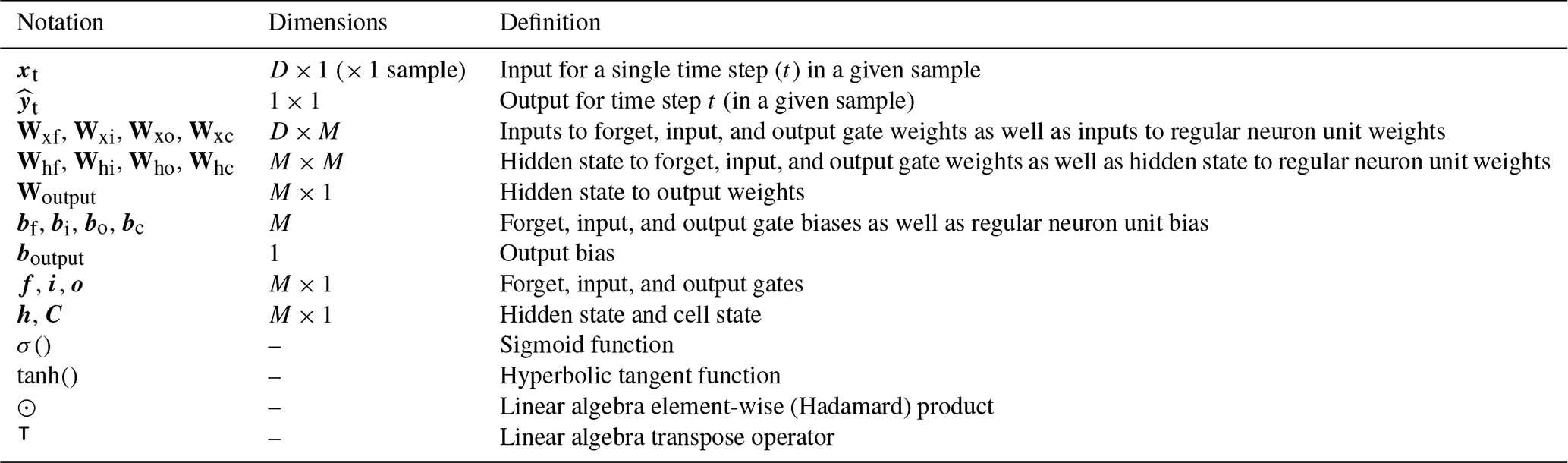
D denotes the total number of features (dynamic and static) for each sample, and M denotes the number of hidden units in the LSTM layer.
Table 2The hyperparameters tested for all LSTMs in the paper and their variations.

3.3 Criteria for performance evaluation
In this paper, to evaluate runoff prediction performance, we use the Kling–Gupta efficiency (KGE) score (Gupta et al., 2009) because it combines the three fundamental diagnostic properties of a predictive hydrologic model, i.e. variability (α), bias (β), and linear correlation (r).
In the above equations, and Y are predicted and true values respectively, and are the mean values of and Y respectively, std is the standard deviation function, and Np is the number of time steps in the period for which we want to calculate the KGE. For example, if we are interested in calculating the KGE on the training data set, Np will be the number of time steps the training data contain. The calculation of the KGE score is catchment-wise throughout the paper.
3.4 Hyperparameter tuning
When addressing a research question using a deep learning model, it is important to limit (as much as possible) any potential conclusion biases resulting from the use of a model that is not hyperparameter tuned. LSTM has, in particular, two interconnected hyperparameters that need to be tuned together: the lookback and hidden unit size. For this purpose, for each LSTM in the paper, we have tested all combinations of all variations in the hyperparameters listed in Table 2 – 6 (lookback variations) × 3 (hidden unit size variations) × 3 (dropout rate variations) = 54 tuning cases. In all of these cases, the batch size, the number of LSTM layers, and the learning rate are constant: 128, 1, and 10−4 respectively.
The remainder of this subsection discusses the choice of and variation in the tuning hyperparameters in this paper.
3.4.1 Learning rate
The gradient-based Adam algorithm (Kingma and Ba, 2017) with a learning rate of 10−4 is used as the optimization algorithm in all experiments. Adam is from the family of algorithms with adaptive learning rates and is considered to be a robust algorithm with respect to the choice of its hyperparameters, including its base learning rate (Goodfellow et al., 2016). A suitable learning rate value would give an asymptotic converging learning (or optimization) curve and would not overshoot effective local minima (Bengio, 2012). Given these factors, Adam's basic learning rate has been fixed to 10−4, and a post hoc examination of the learning curves has been performed for the different models in the different experiments that has not revealed any divergence of the training criteria due to an overly high learning rate. The rate of 10−4, which is 10 times lower than Adam's default base learning rate in Keras, has been selected to provide better steps with respect to local minima. Given this lower chosen learning rate, in order to ensure that full regime training has been provided and that the training criterion has sufficient time to decay, we have not imposed a predetermined number of epochs, instead allowing the LSTM to continue to learn for as long as its performance improves on the validation data. Furthermore, 10−4 has been the chosen value in similar previous studies (Kratzert et al., 2018; Lees et al., 2021).
3.4.2 Dropout rate
The early stopping algorithm implemented in the paper already acts as a regularizer. Goodfellow et al. (2016) show how early stopping is equivalent to L2 regularization in the case of a simple linear model with a quadratic error function and simple gradient descent. Given this, there would be no point testing many dropout variations in our paper.
3.4.3 Batch size
Bengio (2012) notes that the impact of the size of training batches is mostly computational and that, theoretically, it should mainly impact training times and convergence speeds, with no significant impact on test performance. That is, larger batch sizes would speed up computation but need more training in order to arrive at the same error because there are fewer updates per epoch (and vice versa for smaller batch sizes). Typical recommended batch sizes are powers of 2 (as they offer a better GPU runtime), ranging from 32 to 256 (Goodfellow et al., 2016). Very small batch sizes might require a lower learning rate to maintain stability due to the high variance in gradient estimates. Thus, the total runtime could increase significantly. Our chosen learning rate and batch size (10−4 and 128 respectively) gave a reasonable runtime as well as adequate convergence and test performance.
Oudin et al. (2005)Table 3List of the dynamic and static features used in different LSTM models in the paper.

3.4.4 Hidden unit size
Bengio (2012) offers an interesting discussion on the recommended exploration values for a hyperparameter (see the “Scale of values considered” paragraph of Sect. 3.3 of his paper). He explains that, instead of making a linear selection of intermediate-value intervals (the values between the lower and upper bands, here 64 to 256), it is often much more useful to consider a linear or uniform sampling in the log domain – in the space of the logarithm of the hyperparameter. This is because the “ratio” between different values is often more important than their absolute difference when it comes to “the expected impact of the change”. For this reason, Bengio (2012) states that exploring uniformly or regularly spaced values in the space of the logarithm of the numerical hyperparameter is typically to be preferred for positive-valued numerical hyperparameters. Furthermore, should the optimal hidden unit size be lower than 64, using a hidden unit size of 64 would not negatively impact generalization, it would simply require proportionally greater computation (Bengio, 2012).
3.5 Model training and selection of the best hyperparameter set
Here, the goal is to train an LSTM that takes the past T time steps of , …, xt] as the inputs for output , i.e. runoff at time step t (mm d−1). Thus, the input necessarily contains sequences of length T of a number of time-varying forcing variables (dynamic features). In some cases, we wish also to use time-invariant variables (static features), such as physical or climatic catchment attributes. Kratzert et al. (2019b) proposed a variant of LSTM (entity-aware LSTM, or EA-LSTM) that is able to treat static and dynamic features separately from each other. Here, we use a vanilla LSTM and adopt the simplest method of integrating static features – i.e. to repeat each static feature T times to obtain its corresponding sequence and then concatenate the obtained sequences with X. By this means, assuming that D is the total number of features, we will have XT×D. The complete list of dynamic and static features used in this paper is provided in Table 3. Given XT×D and the set of equations presented in Sect. 3.1, the LSTM is thus able to output . If we are in need of runoff predictions for more than one time step, the identical task can be performed for all N time steps, giving N runoff predictions – . Note that, here, N denotes the number of samples in the (mini)batch or batch size, with each sample consisting of a sequence of length T. The goal here is to find the best set of weights W and biases b that map to . By best set, we mean the weights and biases that reduce the overall difference between the LSTM's runoff predictions and runoff true values to a minimum. This overall difference can be measured by a loss function , where Y represents runoff true values. In other words, the goal is to learn the optimal (W,b)opt so that the loss function is globally minimized: or, less formally, .
Depending on whether the LSTM is trained on just a single catchment or on a group of catchments, either the mean squared error (MSE, Eq. 14) or the NSE∗ (Eq. 15) (Kratzert et al., 2019b) is used as the loss function respectively. The NSE∗ is catchment-specific and is of particular use when the input data come from different catchments, producing a potentially wide range of discharge variance. The NSE∗ is normalized with respect to the discharge variance in each catchment. This will prevent smaller or larger weights being assigned to catchments with a lower or higher variance.
In the above equations, B is the number of catchments, and sb is the standard deviation of discharge for catchment b computed using discharges in the training data. Following Kratzert et al. (2019b), ϵ (=0.1) is added to the denominator in Eq. (15) to prevent division by a value very close to 0 in catchments with a very small discharge variance, i.e. when sb→0.
Table 4Names, training catchments, approaches to the selection of the best hyperparameter set, and features used for the five LSTM models in the paper.

We used the Keras library (Chollet et al., 2015) written in Python 3.8 (Van Rossum and Drake, 2009) to build and train all LSTM models in the paper. The Adam algorithm with a learning rate of 10−4 is used as the optimization algorithm in all experiments. All other parameters in the Adam optimization module, including β1 and β2 (L1 and L2 norms), are kept at their default values. To control overfitting, we use the Keras early stopping algorithm. An early stopping algorithm does not impose the same predefined non-traversable number of training epochs on all simulations. It allows the model to continue to learn as long as its performance (here on the validation data) is improving.
The LSTM is trained both locally, using the data from “individual catchments”, and regionally, using the data from “a group of catchments”. In local training, the loss function is the MSE, and only the dynamic features of Table 3 are used. In this paper, LSTMs trained on individual catchments are called SINGLEs, as the data from only a single catchment are used in their training. In regional training, the loss function is the NSE∗, and both dynamic and static features of Table 3 are used. Furthermore, in regional training, all catchments are trained together, once at a national level and once at regime level, with the latter using only catchments belonging to the same regime (see Sect. 2.2). Here, LSTMs trained at the national level are called “REGIONAL NATIONAL” models, and those trained at the regime level are called “REGIONAL REGIME” models. For each of the SINGLE, REGIONAL REGIME, and REGIONAL NATIONAL models, the 54 hyperparameter tuning cases are performed, resulting in the following:
-
361 × 54 individual training sessions for the SINGLEs,
-
54 group training sessions on the 71 Uniform catchments using the REGIONAL REGIME model,
-
54 group training sessions on the 62 Mediterranean catchments using the REGIONAL REGIME model,
-
54 group training sessions on the 101 Oceanic catchments using the REGIONAL REGIME model,
-
54 group training sessions on the 100 Nivo–Pluvial catchments using the REGIONAL REGIME model,
-
54 group training sessions on the 27 Nival catchments using the REGIONAL REGIME model,
-
54 group training sessions on the 361 sample catchments using the REGIONAL NATIONAL model.
This gives a total of 19 818 (= 361 × 54 + 6 × 54) training passes.
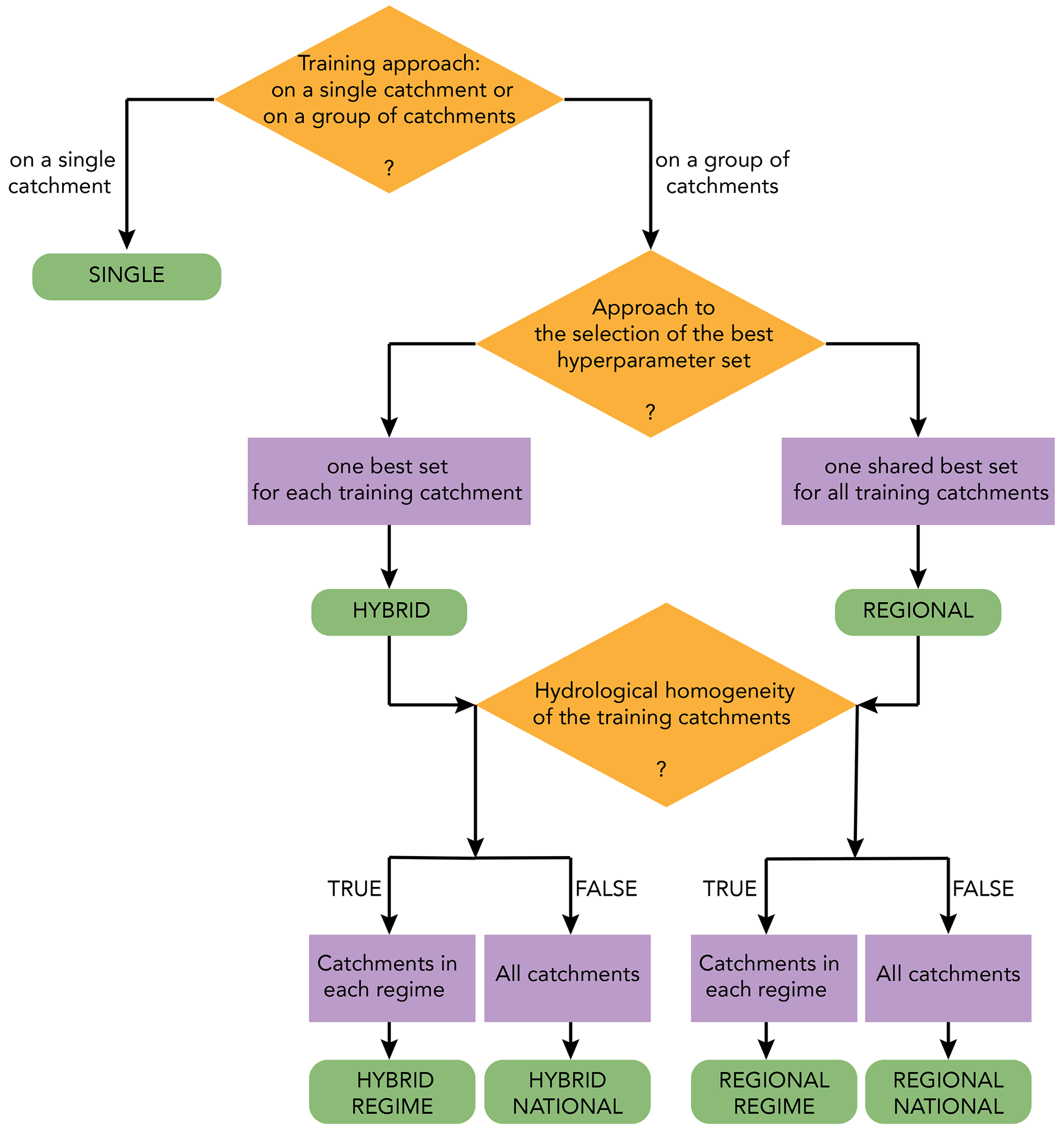
Figure 8Conceptual flowchart of how SINGLE, REGIONAL, and HYBRID LSTM models and their submodels (green rounded rectangles) are built based on three decision criteria (orange rhombuses): the training approach, the approach to the selection of the best hyperparameters, and the training catchments.
So far, different local and regional LSTMs have been trained for the 54 hyperparameter sets. Now, the best hyperparameter set must be chosen for the trained LSTMs. For SINGLEs, the only possible approach is to select, for each catchment, its own best set: the hyperparameter set that offers the best KGE for the validation data. However, for REGIONALs, be they NATIONAL or REGIME, two possibilities exist. We can identify either one best set for each of the training catchments or one best overall set for the entire model. In this paper, we investigate both approaches. By crossing the two (local and regional) training approaches with the two approaches to the selection of the best hyperparameter set (as shown in Fig. 8), we obtain five LSTM models. SINGLEs are trained locally and have locally tuned hyperparameters. REGIONALs are trained regionally, and their best hyperparameter set is also regional. HYBRIDs, as their name suggests, are LSTMs that are trained regionally but whose best hyperparameter set is chosen locally. Table 4 gives a summary of the important features of these models.
3.6 Conceptual benchmark model: GR4J
The daily lumped GR4J model (Génie Rural à 4 paramètres Journalier; Perrin et al., 2003) and its CemaNeige snowmelt routine (Valéry et al., 2014) are selected to benchmark the LSTM. GR4J is chosen for its ability to account for groundwater exchanges with aquifers and/or adjoining catchments thanks to its gain/loss function. This is a distinctive feature of GR4J compared with the benchmark conceptual models used in previous studies (Kratzert et al., 2018; Lees et al., 2021).
GR4J is a parsimonious model incorporating only four free parameters. CemaNeige has two parameters and computes snow accumulation and snowmelt as outputs (Valéry et al., 2014). GR4J is coupled with CemaNeige to perform one simulation for each catchment in the sample. This involves calibration of the coupled model on the training+validation data sets and its evaluation on the test data set. For model calibration, the Michel (Michel, 1989) optimization algorithm is used. For the purpose of comparison with LSTM, the NSE is selected as the objective function for the optimization algorithm. For GR4J, it is recommended that a warm-up period be considered in order to provide the model with an initial state, rather than starting with an arbitrary state (Perrin and Littlewood, 2000). Accordingly, in all simulations, the first 2 years of data are set as the warm-up period when calibrating or evaluating the coupled model. The length of the warm-up period corresponds to the longest lookback tested for the LSTM. All GR4J simulations are performed using the airGR package (Coron et al., 2017, 2020) in the R interface (R Core Team, 2019).
Compulsory inputs to the GR4J model consist of daily total precipitation (mm d−1), potential evapotranspiration (mm d−1) computed using the formula of Oudin et al. (2005), and runoff (mm d−1), where runoff is used only for model calibration. Compulsory inputs to the CemaNeige snowmelt routine are daily total precipitation (mm d−1) and mean air temperature (∘C). The hypsometric data of each catchment are also included as an optional input for the CemaNeige model. It uses this information to account for orographic gradients (Valéry et al., 2014).
Our results showed that the use of a second regularization strategy (dropout rates of 0.2 and 0.4) in conjunction with early stopping would not further improve performance (compared with the use of early stopping alone, i.e. dropout rate of 0). All results presented here correspond to a dropout rate of 0.
4.1 Variations in LSTM performance with respect to input sequence length (lookback)
In Fig. 9, the three curves plot the median KGE scores for the training and validation data sets as well as their average, showing SINGLE (left) and REGIONAL REGIME (right) LSTMs for the five regimes. For each lookback, the median KGE score corresponds to the best hyperparameter set for that lookback. For example, for a lookback of 30 d, selection is made from the following three hyperparameter sets: (lookback = 30, dropout rate = 0, hidden unit size = 64), (lookback = 30, dropout rate = 0, hidden unit size = 128), and (lookback = 30, dropout rate = 0, hidden unit size = 256). We conjecture that the true underlying performance–lookback pattern lies somewhere between the patterns represented by the training and validation curves. The former has the advantage of being used for model training and the latter for hyperparameter selection. In view of this, we have chosen to look at the average of these two curves.
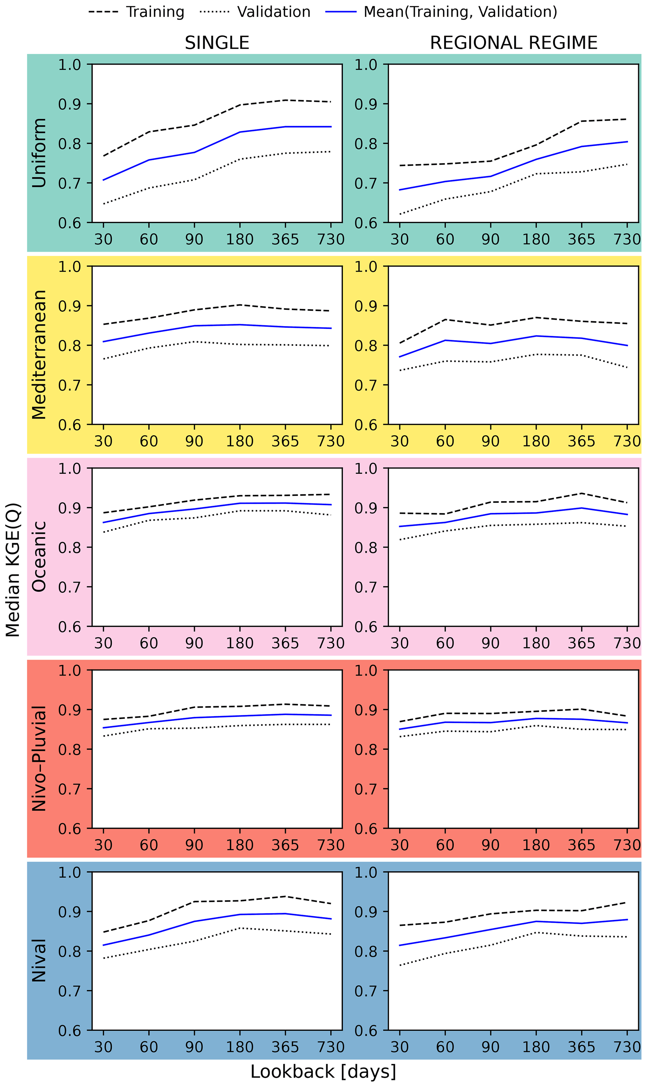
Figure 9LSTM performance variations with respect to the length of input sequences within different regimes for the SINGLE and REGIONAL REGIME models. In each panel, the dashed and dotted lines correspond to the training and validation data respectively. The solid line is the mean of the training and validation lines. Each line plots the median KGE scores (on the y axis) for different lookback sizes (on the x axis). The median KGE score for a given lookback in a given panel is the median of the KGE scores from the panel's catchments.
For both models, the curves tend to show a consistent pattern within the various regimes. The median KGE first increases at a certain slope and then, from a specific lookback onwards, the KGE remains largely unchanged or even decreases. Both the slope and the lookback appear to be regime dependent. In the Uniform and Nival regimes, the slope is distinctively pronounced for both models, and we find the highest sensitivity within these two regimes. In the Mediterranean regime, the median KGE varies between 0.81 and 0.85 and between 0.77 and 0.82 for the SINGLE and REGIONAL REGIME models respectively. The initial slope is steeper in this regime than in the Oceanic regime, and KGE stalls at an earlier point. In both regimes, the global sensitivity of performance to lookback size is low. In the Nivo–Pluvial regime, the initial slope is shallow, creating an almost flat pattern that also reflects low global sensitivity with respect to lookback variations. The range of variation in the median KGE is 0.85–0.89 and 0.85–0.88 for the SINGLE and REGIONAL REGIME models respectively.
The continuous tendency for performance to improve with increasing lookback up to lookbacks longer than a year within the Uniform regime, as compared to the multi-month scale in other regimes, is consistent with the multi-year and multi-month catchment memory scales showed by de Lavenne et al. (2021) for the Uniform and non-Uniform catchments in the French context.
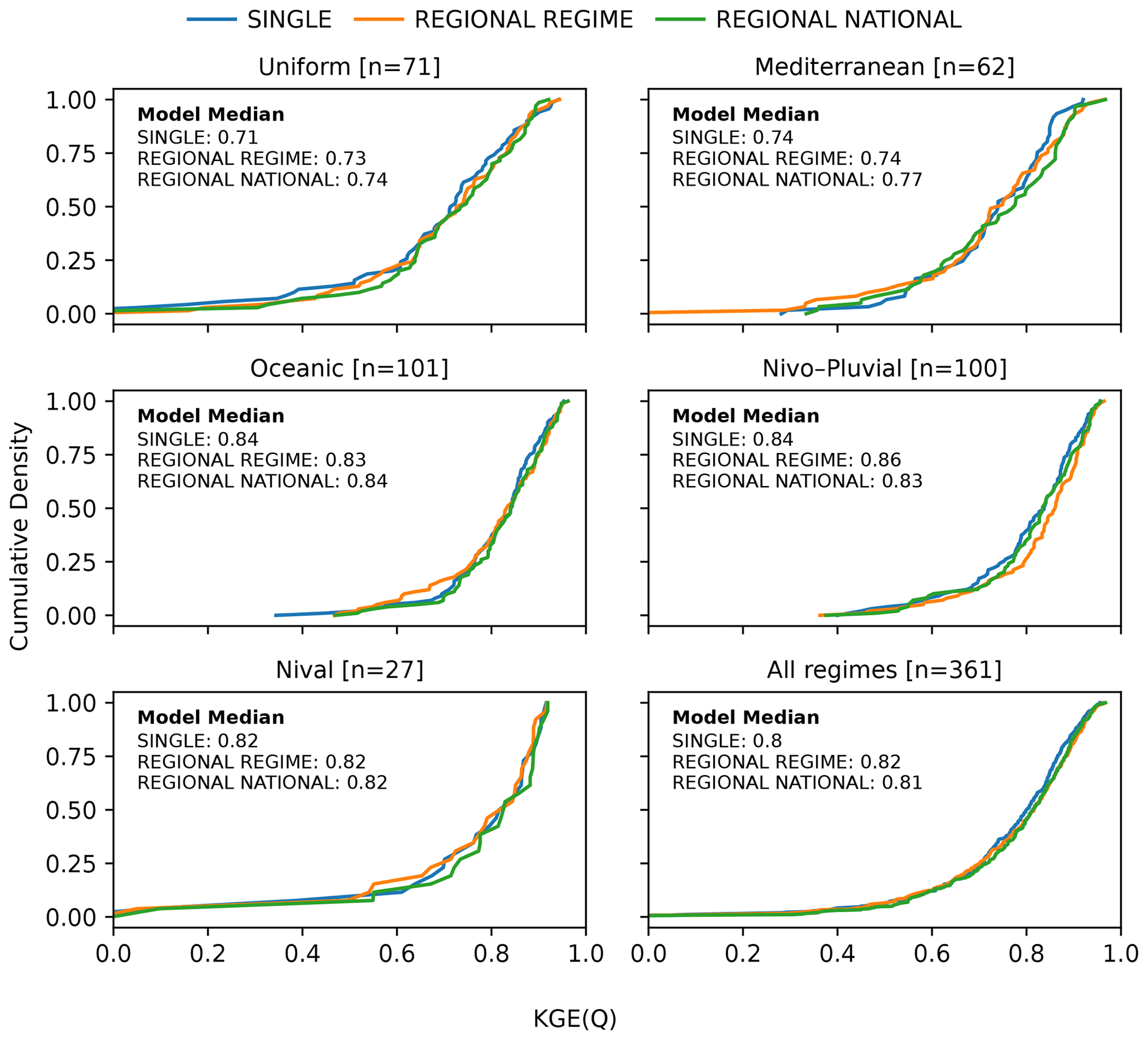
Figure 10Cumulative distribution functions (CDFs) of the KGE scores of the test data for three LSTM models: SINGLE (blue), REGIONAL REGIME (orange), and REGIONAL NATIONAL (green). From top to bottom, the first five panels indicate the CDFs of one of the five regimes: Uniform, Mediterranean, Oceanic, Nivo–Pluvial, and Nival. The last panel corresponds to the distributions of the entire sample.
4.2 Variations in LSTM performance by training approach
Figure 10 compares the cumulative distribution function (CDF) of the KGE for the locally trained SINGLE, REGIONAL REGIME, and REGIONAL NATIONAL LSTMs (see Fig. 8 and Table 4 for their description). First comparing the median KGE for local training with that of regional training (both regime and national levels), regional training outperforms local training in almost all regimes. However, except in the Uniform regime, the difference in performance between the SINGLE model and the best REGIONAL model remains minor. Overall, if we take all catchments into account, the median KGE is 0.80 for the SINGLE model versus 0.82 and 0.81 for the REGIONAL REGIME and REGIONAL NATIONAL models respectively.
Next, homogeneous group training (REGIONAL REGIME) is specifically compared with non-homogeneous group training (REGIONAL NATIONAL). In the Mediterranean catchments, the REGIONAL REGIME model is observed to have a lower median KGE than the REGIONAL NATIONAL model, whereas it is higher in the Nivo–Pluvial regime. In all other regimes, both training types have almost the same median KGE. In the Nivo–Pluvial regime, the CDF of the REGIONAL REGIME model is completely shifted towards higher KGE scores. In the Nival regime, although both models have the same median KGE, the CDF curve of the REGIONAL NATIONAL regime is shifted towards better KGEs. Overall, when all catchments are considered, the homogeneous group training slightly outperforms the group training with mixed regimes in terms of the median KGE score. However, their CDFs are superposed for high KGEs.
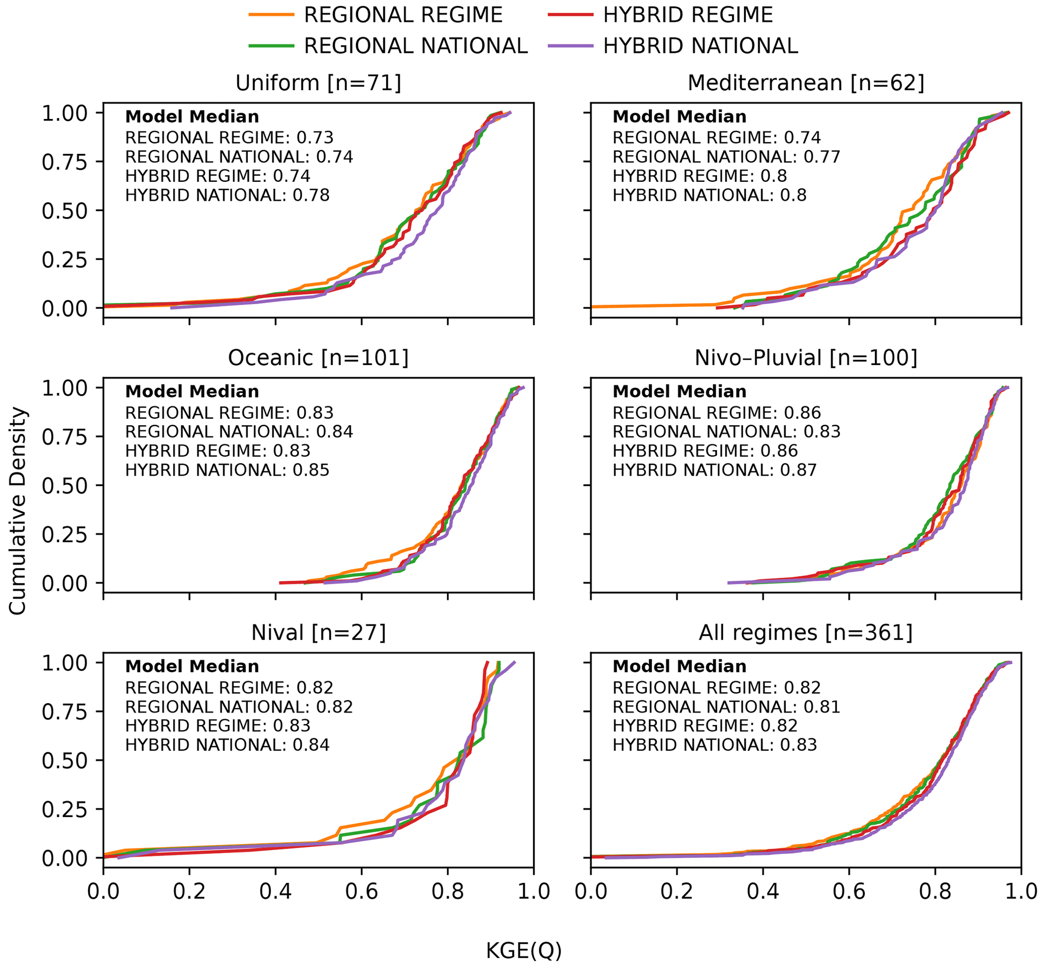
Figure 11Cumulative distribution functions (CDFs) of the KGE scores of the test data for the group-trained LSTM models: REGIONAL REGIME (orange), REGIONAL NATIONAL (green), HYBRID REGIME (red), and HYBRID NATIONAL (purple). From top to bottom, the first five panels indicate the CDFs for each of the five regimes: Uniform, Mediterranean, Oceanic, Nivo–Pluvial, and Nival. The last panel corresponds to the distributions of the entire sample.
4.3 Variations in LSTM performance by approach to best hyperparameter set selection
Figure 11 compares the CDFs for the group-trained REGIONAL and HYBRID LSTMs, which differ with respect to their approach to the selection of their best hyperparameter set. Thus, the HYBRID models benefit from the advantages of group training and the use of local hyperparameters.
We see that there is clearly a performance improvement from the REGIONAL NATIONAL model to the HYBRID NATIONAL model in almost all regimes as well as overall. This is both in terms of median KGE scores and the shift in the CDF curve towards better KGEs. However, moving from the REGIONAL REGIME model to the HYBRID REGIME model, there is little or no improvement in performance, except for the Mediterranean regime. Of all tested LSTMs, the HYBRID NATIONAL model performs best.
Table 5Median KGE scores, within different regimes and overall, for the GR4J model compared to the LSTM models.
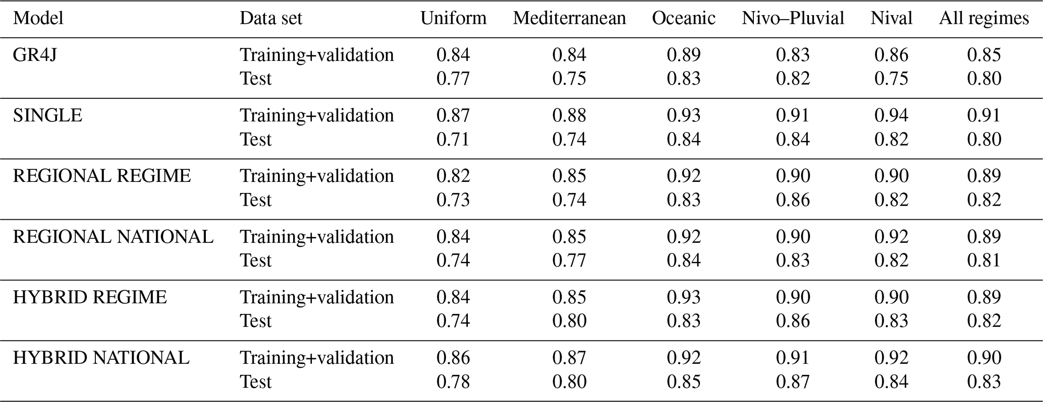
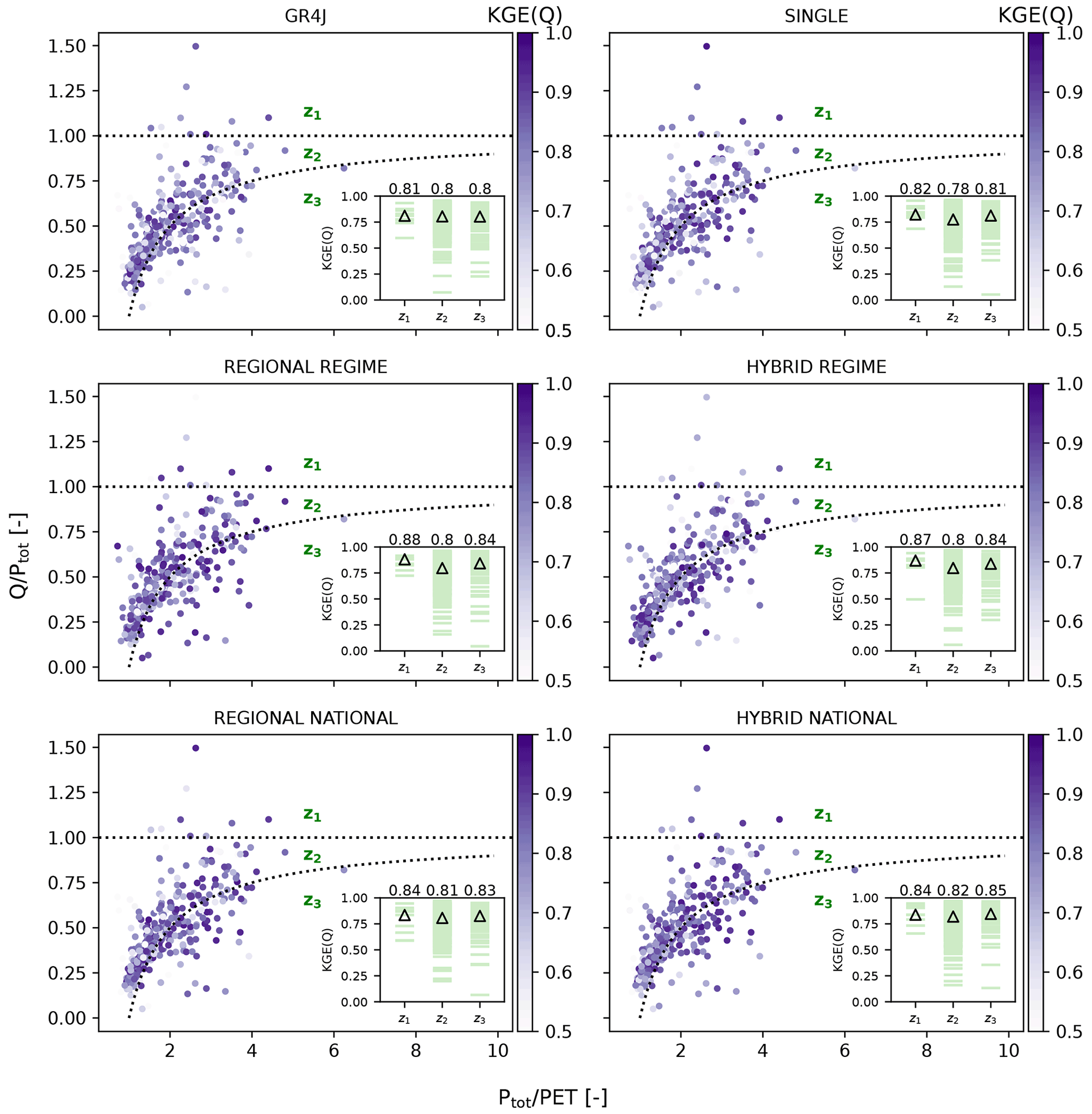
Figure 12Variation in KGE scores with respect to the runoff ratio () and wetness index () for the GR4J and LSTM models. Scores lower than 0.5 are shown in the same tone as the lower extreme of the colour bar. The inset plot within each panel shows the KGE scores of the catchments located in each of the z1 (above the horizontal water limit line), z2 (between the horizontal and curved lines), and z3 (below the curved line) zones. The (△) symbol and numbers in the inset plots represent the median KGE scores of the three zones. The KGE scores correspond to the test data, with the exception of the first 2 years, which constitute the warm-up period in GR4J and for which there are no outputs.
4.4 Performance comparison between LSTMs and the GR4J model
Table 5 compares the median KGE scores from the GR4J model with the LSTM models for the training+validation and test periods. We see from the table that GR4J is generally more robust than local and regional LSTMs. Looking at the median KGE score across different regimes for the test period, with the exception of the Uniform and Mediterranean regimes, all LSTMs outperform GR4J or have the same score, with the latter occurring in only two cases. In the Mediterranean regime, GR4J outperforms only the SINGLE LSTM. Overall, taking all catchments from different regimes into account, SINGLE and GR4J models have similar scores, whereas the group-trained LSTMs outperform the GR4J model, although the performance difference is small. Group-trained LSTMs in previous studies (Kratzert et al., 2019b; Lees et al., 2021) also had better overall performance when compared with conceptual local models, although the LSTM's higher performance in these studies was more pronounced. One possible explanation could be the difference between GR4J and the conceptual models used in the previous studies including SAC-SMA, the Framework for Understanding Structural Errors (FUSE) (Clark et al., 2008), ARNOVIC, TOPMODEL (Bracken and Croke, 2007), and the Precipitation–Runoff Modelling System (PRMS) (Leavesley et al., 1983). These models are explicitly mass conservative – unlike GR4J, which is explicitly designed to capture water losses and gains through an exchange parameter (Perrin et al., 2003). Thus, GR4J is able to simulate runoff in catchments where the water balance is not closed. Figure 12 shows a diagnostic plot of the runoff coefficient (= ) versus wetness index WI (= ) for the 361 catchments. The points – representing the catchments – are shaded according to the KGE score. Of the 361 catchments plotted in each panel of Fig. 12, 9 catchments fall in zone z1 (above the horizontal water limit line). Given that Q>Ptot in this zone, there is a surplus in the catchment's water balance; therefore, it does not close. The z2 zone (located between the horizontal and curved lines) contains 255 catchments in which the water balance is satisfied. Finally, 97 catchments fall in the z3 zone (located below the curved line) where the water balance does not close, as and, therefore, , indicating a potential water deficit. The inset in each panel shows the KGE scores of the catchments located in each of the z1, z2, and z3 zones, along with their median values. In z1 and z3, where the water balance is not satisfied, median scores in the GR4J model are the same or better than z2, where there is water balance closure. This contrasts with the corresponding finding of the previous study by Lees et al. (2021). Interestingly, we can observe the same but clearer pattern for the LSTMs: the median KGE score for all LSTMs is lower in z2 than in z1 and z3. For catchments in the z1 zone, the REGIME LSTMs clearly outperform NATIONAL and SINGLE LSTMs. Within z3, the group-trained models produce similar scores, which are better than the corresponding scores of the SINGLE model. Considering the fact that the 136 catchments in this zone have either a surplus (9 catchments) or deficit (97 catchments) in their water balance, we note that the median KGE scores for LSTM models are better than those for GR4J: 0.81 (SIMPLE), 0.84 (REGIONAL REGIME), 0.84 (HYBRID REGIME), 0.83 (REGIONAL NATIONAL), and 0.84 (HYBRID NATIONAL) versus 0.80 (GR4J). This agrees with the corresponding better overall performance of the LSTMs over the four conceptual models in catchments without water closure in Lees et al. (2021).
5.1 Does the LSTM performance–lookback pattern depend on the catchment regime?
The Uniform and Nival regimes can be distinguished as the two regimes with the cleanest performance–lookback pattern, where performance increases with increasing lookback size. We can relate this to the long-term dynamics of their dominant hydrologic processes: the recharge and discharge of the aquifer and the thawing of accumulated snow.
Uniform catchments occur mainly in areas known to be highly influenced by large aquifers, such as the aquifers of the Seine or the Somme river basins in the north of France (Fig. 3). Such aquifers can significantly modify the temporal dynamics of the impacted catchments and widely hamper the correlation of runoff with current hydroclimatic conditions (Fig. 4). Runoff at the outlets of Uniform catchments can depend on precipitations from several years earlier (de Lavenne et al., 2021). In snow-dominated catchments, precipitation is stored as snow, which is later released (as snowmelt) during the late spring/early summer.
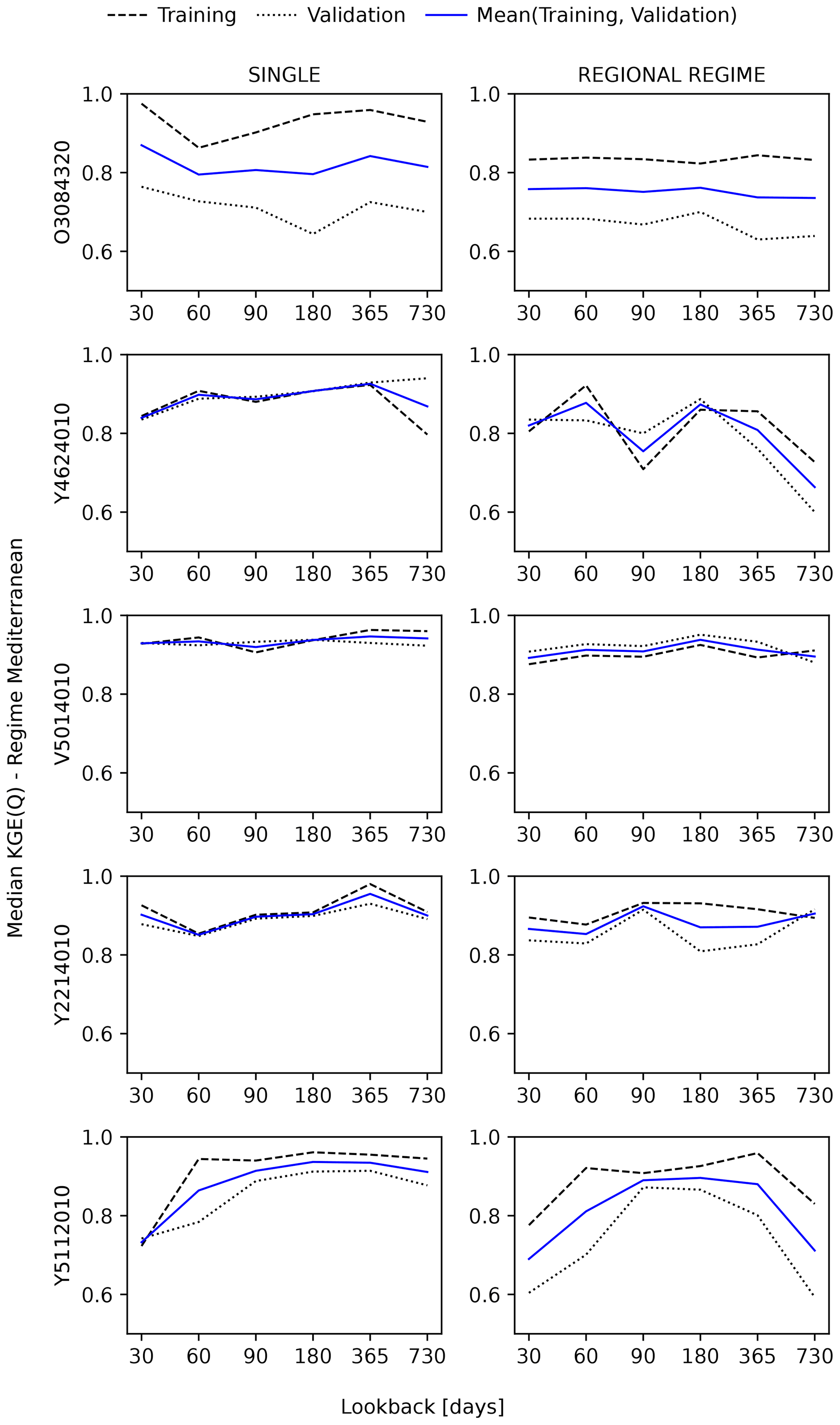
Figure 13Five examples from the Mediterranean regime, each with a different lookback sensitivity pattern.
In the Mediterranean regime, the performance–lookback pattern is characterized by a narrow spread in the KGE scores for different lookbacks, whereas a clear offset was expected for small lookback values. In this regime, internal states (e.g. soil moisture) do not depend on long antecedent periods, as precipitation tends to generate flash floods and is particularly intense in the autumn (Fig. 4). Although we see a mild tendency for lookback values of 90 and 60 d for local and regional LSTMs, at both scales, the KGE scores vary within a narrow range regardless of lookback choice. One explanation would be that various levels of lookback sensitivity may exist for different catchments within this regimes due to inter-regime differences in characteristics such as, soil type, bedrock geology, drainage class, and so forth. For examples of such variability, the reader is referred to Fig. 13. After further investigation, we note that many of Mediterranean catchments are situated in karstic regions that might exert an influence, albeit very locally, on their temporal dynamics. We have not investigated this hypothesis further in this paper. However, should this be the case, we can relate the unclear pattern in this regime to the absence of one single dominant process; instead, dominant processes are combined to different degrees in the various catchments.
In the Oceanic and Nivo–Pluvial regimes, the performance–lookback pattern displays little variation, and there is far less sensitivity to lookback in the median KGE scores. We attribute this to the intermediate-term dynamics of the dominant hydrologic processes in these two regimes.
5.2 How good is the LSTM trade-off between generalization and precision when passing from local to regional training?
To answer this question, we need to take SINGLE, REGIONAL REGIME, and REGIONAL NATIONAL LSTMs into account. In the passage from individual catchment (local) training to group (regional) training, we increased the capacity of the model (by adding 10 static attributes) and the size of the data. As a result, LSTM performance improved in almost all regimes and overall. That is, in passing both from local to homogeneous regional training and from local to heterogeneous regional training, the precision that the LSTM gains is “almost” always greater than the generalization it loses. For Uniform, Mediterranean, and (to a lesser extent) Nivo–Pluvial catchments, the passage from local to at least one of the regional LSTMs is a real gain. For the two other regimes, the benefit is less obvious, and performance improvements do not turn out to be significant.
One explanation for the small performance difference between local and regional (homogeneous or heterogeneous) training is that the quantity of available data at the local level is already sufficiently large with respect to the complexity of catchment representations. Thus, the LSTM has already “asymptoted” to an error very close to the minimum possible error. At the regional level, although the amount of data has increased greatly, the result of the gained precision, lost generalization, and varied complexity is not sufficiently positive to push the final error to a point closer to the minimum possible error. Additionally, in local training, selection of the best hyperparameter set is also local (catchment-wise), allowing each catchment to take its own best set.
5.3 Is there a performance gain for regional LSTMs when passing from hydrologically heterogeneous to homogeneous training and vice versa?
To answer this question, we need to compare the REGIONAL REGIME model against the REGIONAL NATIONAL model. For almost all regimes as well as overall, when hydrologically similar but fewer catchments are used, median KGE scores are as good as when far more training catchments from various regimes are used. This is interesting for at least two reasons.
First, both models benefit from group training, and their data are already several times greater than local-level data. However, of the two, it is not the model with greater amount of training data that performs best. For example, in the Nival regime, the (heterogeneous) national model uses data “13 times” larger than the data used by the (homogeneous) regime model. Nevertheless, they have the same median KGE score. The point to note here is that, passing from the regime level to national level, we did not increase the data from this particular regime (representation) 13 times. We did add a considerable amount (13 times the regime size) of data from some “dissimilar” representations. This is very different from including a large quantity of data from the “similar” representation, as occurs in the passage from local to regime training. Therefore, for non-homogeneous training there is a “varied”, but not necessarily an added, complexity with respect to the representations.
Second, for both forms of training, the complexity (and learning capacity) of the model is the same – exactly the same model with identical static attributes is used for both forms of training. In regime (homogeneous) training, each REGIME LSTM learns a single representation, whereas the LSTM is exposed to the representations from all regimes in national (non-homogeneous) training.
What appears to be important for both models is whether the varied complexity is shifted towards a simpler or a more difficult learning representation. In the latter case, it is then important whether there is sufficient data. The complexity of representation(s) appears to vary from regime to regime. Given our results, we can identify three levels:
-
The first level is regimes with “self-sufficient” representations where homogeneous training clearly outperforms heterogeneous training. The only instance of this level is found in the Nivo–Pluvial regime. In this regime, the new complexity appears to be shifted towards a “more complex” representation.
-
The second level is regimes with “self-insufficient” representations, which must have inputs from contrasting/dissimilar representations to be learned by the LSTMs. The only instance of this level is the Mediterranean regime.
-
The third level is regimes with “neutral” representations for which the addition/removal of contrasting representations has little or no effect on the complexity of the task for LSTM. The Uniform, Oceanic, and Nival regimes exhibit this level of representation. However, if we look at the performance overall, it turns out that almost the same level of data adequacy–representation complexity is achieved in both regime and national training forms.
One other important point to note is that the non-homogeneous (NATIONAL) LSTMs are “regime-informed”. That is, although their data derive from all regimes, identical variables to those used to classify the regimes are then input to the NATIONAL LSTMs as static attributes. Therefore, the latter are not absolutely naive with respect to the non-homogeneity of data. Given this regime-informed property, we conjecture that, to some unknown but positive extent, NATIONAL LSTMs already have the capacity to extract the classification. A systematic investigation is required to prove this. Should it indeed turn out to be the case, it would have the great advantage of making NATIONAL LSTMs classification-free; thus, there would be no need to encode the classification thresholds and conditions separately. Nevertheless, a national data set is still required to train them.
In our results, we did not observe the performance improvement that Fang et al. (2022) obtained when they passed from LSTMs trained on single spatial ecoregions to the LSTM trained on all ecoregions. There are a number of explanations for this difference. The measures of similarity used in the two studies are very different. We have used purely hydrologic measures to classify catchments, whereas Fang et al. used the “spatial proximity” measure of similarity in their experiments. The climatic context as well as the data sets and their size are also very different in the two studies.
5.4 What is the most effective way of using LSTMs to predict runoff?
Our results suggest that the performance of an LSTM-based runoff model is controlled by two factors: (1) its training approach and (2) its lookback–hidden unit size tuning. The results of this paper suggest that maximization of the number of training catchments (national-scale training) in conjunction with local selection of the lookback–hidden unit size set give the best results, both within the regimes and overall. The interesting point to note is that it is only the “combination” of the two components of this setting that gives the best results. Either of them separately does not appear to be a major winning factor: local LSTMs with local lookback–hidden unit size sets did not outperform regional LSTMs, and NATIONAL LSTMs did not outperform REGIME LSTMs. We should also remember that the NATIONAL LSTMs that we tested are regime-informed. Thus, we might include this property as the third component of this setting.
We have previously discussed the importance of lookback as a hyperparameter for LSTM. Here, we note the importance of tuning lookback and hidden unit size at a local scale so that the LSTM can better capture the dynamics of each catchment separately. The relationship between these two hyperparameters has been previously recognized by Kratzert et al. (2019a).
In this study, we have used a sample of 361 gauged catchments in the hydrologically diverse French context. Our goal has been to exploit catchment hydrologic information when using LSTM-based runoff models. Thus, we have proposed a regime classification built on three hydrologic indices to identify catchments with similar hydrologic behaviours (representations). We have then trained the LSTM once locally – on individual catchments – and once regionally – on a group of catchments. We have performed the regional training at two scales: (1) at the scale of each hydrologic regime (i.e. only catchments from the same regime have been trained together) and (2) at the national scale (i.e. all 361 catchments have been trained together). For all training passes, we have performed 54 hyperparameter tunings on three hyperparameters: the dropout rate (three variations) as well as the two important LSTM hyperparameters, namely input sequence length (six variations) and hidden unit size (three variations). We have investigated the relationship between the size of an LSTM's input sequence and LSTM performance within different regimes. We have tested a new approach to the selection of the best hyperparameter set for regional LSTMs, and we have examined how different training and hyperparameter selection approaches change the performance of LSTM. For training and evaluation of all local and regional LSTMs, we have used three long completely independent data sets: training (10 ≤ ≤ 40 years), validation (10 years), and test (10 years). In both local and regional training, we have implemented the early stopping algorithm with no predefined number of training epochs, allowing the LSTM to continue to learn for as long as its performance improves on the validation data. The results of our paper suggest the following main conclusions:
-
In the Uniform and Nival regimes, where there is a clean long-term dominant process, we found a clear performance–lookback pattern, with performance increasing with increasing lookback up to an effective value, which depended on the time scaling of the dominant process. In the Mediterranean regime, characterized by its propensity to generate flash floods, we expected a similar distinct pattern but with a much shorter effective lookback. What we found was a narrow spread of performance scores for different lookbacks. We assumed this to relate to the underlying different temporal dynamics in this regime, given that several catchments in this regime might be locally affected by the presence of karstic geological features.
In the Oceanic and Nivo–Pluvial regimes, we found a largely unchanging performance–lookback pattern, reflecting performance insensitivity to changes in lookback values. This indicates that, in these regimes, adequate performance can be achieved without using large lookbacks.
-
Whether an LSTM benefits from the passage from local to regional or not depends on (a) the amount of data at the local scale and (b) how it can negotiate the trade-off between the varied complexity of the representation(s) to be learned and the augmented data at the regional scale. If, in the move from local to regional, there is also an increase in model complexity produced, for example, by the inclusion of multiple attributes in the regional model, this trade-off could become harder because the LSTM would need to further trade generalization for precision (due to the more complex model). The passage from local to regime level produced a slightly better performance improvement than did the passage from local to national level.
-
At the local scale of a single catchment, if the representation to be learned is “smooth” enough to elicit, or if the catchment's data are so abundant that there is no difficulty in eliciting whatever complex representation they contain, the LSTM will already be very close to the minimum possible error. In such cases, there will be “less room” to improve performance by passing to regional LSTMs.
-
At the regional scale, from the regime (hydrologically homogeneous) level to the national (hydrologically heterogeneous) level, the model capacity is the same. A large quantity of dissimilar data are added, thereby varying the complexity of the new representations to be learned. What appears to be important is whether the varied complexity is shifted towards a simpler or a more difficult learning representation. In the latter case, the issue is then whether there is an adequate quantity of data. Our results showed regime training to perform better overall, but the difference was very slight, and we can consider the two forms of regional training to be equivalent. This means that, for both regime and national training levels, the quantity of data has been adequate and appropriate with respect to the complexity of the representation(s) at that level. Nevertheless, the potential role of our national LSTM's regime-informed property in simplifying the task in the heterogeneous space should not be excluded.
-
Given the almost equivalent performance of REGIME and regime-informed NATIONAL LSTMs, in choosing between them, we may take into consideration that the former needs less data but requires an external classification – a precise encoding of our knowledge to the right classification. The latter requires a national database but calls for no classification (criterion).
-
To improve the performance of an LSTM model, two elements were found to be important: the training approach and the lookback–hidden unit size tuning. The best performance was shown by the HYBRID NATIONAL LSTMs, mixing national training with local tuning of the two lookback, hidden unit size hyperparameters, and providing regime information through attributes.
Our findings allow us to identify a number of directions for further research:
-
The conclusions drawn here have been premised on a single condition concerning the similarity and size of data. References to an “increase in data size” at the national training level designated an increase in the data of dissimilar representations with the increase always falling within the following bands: times (Oceanic regime) to times (Nival regime). We encourage further investigations where the degree of dissimilarity and size of data are systematically altered in a controlled environment.
-
A useful step for the improvement of homogeneous training would be to refine the current classification to maximize the number of self-sufficient regimes.
-
Our hydrologically heterogeneous LSTMs were regime-informed. We encourage verification of the conjecture that an LSTM is able to learn classification if we provide it with regime information (through classification attributes). A simple way to achieve this is to include once and exclude once the classification indices in and from static features of regional LSTMs and compare the results. This paper does the former but not the latter.
-
A future research direction could be to explore the relationship between LSTM's optimal lookback and memory-related metrics, such as the catchment forgetting curve (de Lavenne et al., 2021), for each individual catchment. This would allow us to predict the optimal lookback for each catchment.
-
The methods presented in this paper are developed for gauged catchments. A further step would be to extend them to approaches applicable to ungauged catchments – catchments not used in training.
To request access to the results and the codes upon which this study is based, please contact the corresponding author.
The meteorological forcing data are produced and provided by Météo France (Quintana-Segui et al., 2008; Vidal et al., 2010). The hydrometric data are collected and provided by the French Ministry of Environment. These two data sources are processed and compiled into a single data base (HydroClim, https://doi.org/10.15454/UV01P1; Delaigue et al., 2020), which is used in this study. To request access to the data, please contact the data owners: Météo France (https://donneespubliques.meteofrance.fr/; Météo France, 2022) for the meteorological data, Banque Hydro (https://hydro.eaufrance.fr/edito/a-propos-de-lhydroportail; French Ministry of Environment, 2022) for the hydrometric data, and INRAE's HYCAR research team (https://doi.org/10.15454/UV01P1; Delaigue et al., 2020) for the HydroClim data set.
RH designed all of the experiments with advice from PB, PAG, and PJ. RH conducted all of the experiments and wrote the manuscript. PB gave guidance on the data and GR4J simulations. PAG assisted RH with the execution of experiments. PJ supervised the work and was in charge of the overall direction. Analysis of the results and revision of the manuscript were carried out collectively.
The contact author has declared that none of the authors has any competing interests.
Publisher's note: Copernicus Publications remains neutral with regard to jurisdictional claims in published maps and institutional affiliations.
This work was granted access to the IDRIS GPU resources under the allocation 2022-AD011013339 made by GENCI. We would like to extend our sincere thanks to Jérémy Verrier for his constant support and help with respect to using INRAE and GENCI's HPC resources. We would also like to thank our handling editor (Efrat Morin), John Quilty, and the two anonymous referees, who provided input that substantially improved this paper.
This paper was edited by Efrat Morin and reviewed by John Quilty and two anonymous referees.
Beck, C., Jentzen, A., and Kuckuck, B.: Full error analysis for the training of deep neural networks, Infin. Dimens. Anal. Qu., 25, 2150020, https://doi.org/10.1142/S021902572150020X, 2022. a
Bengio, Y.: Practical recommendations for gradient-based training of deep architectures, in: Neural networks: Tricks of the trade, edited by: Montavon, G., Orr, G. B., and Müller, K.-R., Springer, 437–478, https://doi.org/10.1007/978-3-642-35289-8_26, 2012. a, b, c, d, e
Bracken, L. J. and Croke, J.: The concept of hydrological connectivity and its contribution to understanding runoff-dominated geomorphic systems, Hydrol. Process., 21, 1749–1763, https://doi.org/10.1002/hyp.6313, 2007. a
Burnash, R. J. C., Ferral, R. L., and McGuire, R. A.: A generalized streamflow simulation system: Conceptual modeling for digital computers, Cooperatively developed by the Joint Federal-State River Forecast Center, United States Department of Commerce, National Weather Service, State of California, Department of Water Resources, https://books.google.fr/books?hl=en&lr=&id=aQJDAAAAIAAJ&oi=fnd&pg=PR2&dq=A+generalised+streamflow+simulation+system+conceptual+modelling+for+digital+computers.,+Tech.+rep.,+US+Department+of+Commerce+National+Weather+Service+and+State+of+California+Department+of+Water+Resources&ots=4tUeYd75bu&sig=9E64OzUeZxuyF4ULMgxbQyr9ktI&redir_esc=y#v=onepage&q&f=false) (last access: 16 November 2022), 1973. a
Chiverton, A., Hannaford, J., Holman, I., Corstanje, R., Prudhomme, C., Bloomfield, J., and Hess, T. M.: Which catchment characteristics control the temporal dependence structure of daily river flows?, Hydrol. Process., 29, 1353–1369, https://doi.org/10.1002/hyp.10252, 2015. a
Chollet, F. et al.: Keras, GitHub, https://github.com/fchollet/keras (last access: 2 November 2022), 2015. a
Clark, M. P., Slater, A. G., Rupp, D. E., Woods, R. A., Vrugt, J. A., Gupta, H. V., Wagener, T., and Hay, L. E.: Framework for Understanding Structural Errors (FUSE): A modular framework to diagnose differences between hydrological models, Water Resour. Res., 44, W00B02, https://doi.org/10.1029/2007WR006735, 2008. a
Coron, L., Thirel, G., Delaigue, O., Perrin, C., and Andréassian, V.: The Suite of Lumped GR Hydrological Models in an R package, Environ. Modell. Softw., 94, 166–171, https://doi.org/10.1016/j.envsoft.2017.05.002, 2017. a
Coron, L., Delaigue, O., Thirel, G., Perrin, C., and Michel, C.: airGR: Suite of GR Hydrological Models for Precipitation-Runoff Modelling, R package version 1.4.3.65, https://CRAN.R-project.org/package=airGR (last access: 2 November 2022), 2020. a
Delaigue, O., Génot, B., Lebecherel, L., Brigode, P., and Bourgin, P.-Y.: Database of watershed-scale hydroclimatic observations in France, Recherche Data Gouv [data set], https://doi.org/10.15454/UV01P1, 2020. a, b, c
de Lavenne, A., Andréassian, V., Crochemore, L., Lindström, G., and Arheimer, B.: Quantifying multi-year hydrological memory with Catchment Forgetting Curves, Hydrol. Earth Syst. Sci., 26, 2715–2732, https://doi.org/10.5194/hess-26-2715-2022, 2022. a, b, c, d
Fang, K., Kifer, D., Lawson, K., Feng, D., and Shen, C.: The Data Synergy Effects of Time-Series Deep Learning Models in Hydrology, Water Resour. Res., 58, e2021WR029583, https://doi.org/10.1029/2021WR029583, 2022. a, b, c, d, e, f
Feng, D., Fang, K., and Shen, C.: Enhancing streamflow forecast and extracting insights using long-short term memory networks with data integration at continental scales, Water Resour. Res., 56, e2019WR026793, https://doi.org/10.1029/2019WR026793, 2020. a
Frame, J. M., Kratzert, F., Klotz, D., Gauch, M., Shalev, G., Gilon, O., Qualls, L. M., Gupta, H. V., and Nearing, G. S.: Deep learning rainfall–runoff predictions of extreme events, Hydrol. Earth Syst. Sci., 26, 3377–3392, https://doi.org/10.5194/hess-26-3377-2022, 2022. a
French Ministry of Environment: Hydro Portail, https://hydro.eaufrance.fr/edito/a-propos-de-lhydroportail, last access: 9 November 2022. a
Gao, S., Huang, Y., Zhang, S., Han, J., Wang, G., Zhang, M., and Lin, Q.: Short-term runoff prediction with GRU and LSTM networks without requiring time step optimization during sample generation, J. Hydrol., 589, 125188, https://doi.org/10.1016/j.jhydrol.2020.125188, 2020. a
Gauch, M., Kratzert, F., Klotz, D., Nearing, G., Lin, J., and Hochreiter, S.: Rainfall–runoff prediction at multiple timescales with a single Long Short-Term Memory network, Hydrol. Earth Syst. Sci., 25, 2045–2062, https://doi.org/10.5194/hess-25-2045-2021, 2021a. a, b
Gauch, M., Mai, J., and Lin, J.: The proper care and feeding of CAMELS: How limited training data affects streamflow prediction, Environ. Modell. Softw., 135, 104926, https://doi.org/10.1016/j.envsoft.2020.104926, 2021b. a, b, c
Goodfellow, I., Bengio, Y., and Courville, A.: Deep Learning, MIT Press, ISBN 9780262337373, 2016. a, b, c, d, e, f, g, h
Gupta, H. V., Kling, H., Yilmaz, K. K., and Martinez, G. F.: Decomposition of the mean squared error and NSE performance criteria: Implications for improving hydrological modelling, J. Hydrol., 377, 80–91, https://doi.org/10.1016/j.jhydrol.2009.08.003, 2009. a
Haines, A., Finlayson, B., and McMahon, T.: A global classification of river regimes, Appl. Geogr., 8, 255–272, https://doi.org/10.1016/0143-6228(88)90035-5, 1988. a
Hochreiter, S.: The vanishing gradient problem during learning recurrent neural nets and problem solutions, Int. J. Uncertain. Fuzz., 6, 107–116, https://doi.org/10.1142/S0218488598000094, 1998. a
Hochreiter, S. and Schmidhuber, J.: Long Short-Term Memory, Neural Comput., 9, 1735–1780, https://doi.org/10.1162/neco.1997.9.8.1735, 1997. a
Kachroo, R. and Natale, L.: Non-linear modelling of the rainfall-runoff transformation, J. Hydrol., 135, 341–369, https://doi.org/10.1016/0022-1694(92)90095-D, 1992. a
Kingma, D. P. and Ba, J.: Adam: A Method for Stochastic Optimization, https://doi.org/10.48550/arXiv.1412.6980, 2017. a
Kratzert, F., Klotz, D., Brenner, C., Schulz, K., and Herrnegger, M.: Rainfall–runoff modelling using Long Short-Term Memory (LSTM) networks, Hydrol. Earth Syst. Sci., 22, 6005–6022, https://doi.org/10.5194/hess-22-6005-2018, 2018. a, b, c, d, e, f, g, h, i, j
Kratzert, F., Klotz, D., Herrnegger, M., Sampson, A. K., Hochreiter, S., and Nearing, G. S.: Toward Improved Predictions in Ungauged Basins: Exploiting the Power of Machine Learning, Water Resour. Res., 55, 11344–11354, https://doi.org/10.1029/2019WR026065, 2019a. a, b, c
Kratzert, F., Klotz, D., Shalev, G., Klambauer, G., Hochreiter, S., and Nearing, G.: Towards learning universal, regional, and local hydrological behaviors via machine learning applied to large-sample datasets, Hydrol. Earth Syst. Sci., 23, 5089–5110, https://doi.org/10.5194/hess-23-5089-2019, 2019b. a, b, c, d, e, f, g, h, i
Leavesley, G. H., Lichty, R. W., Troutman, B. M., and Saindon, L. G.: US Geological Survey Water Resources Investigations, Water-Resources Investigations Report 83-4238, USGS, https://pubs.usgs.gov/wri/1983/4238/report.pdf (last access: 8 November 2022), 1983. a
LeCun, Y.-A., Bottou, L., Orr, G.-B., and Müller, K.-R.: Efficient backprop, in: Neural networks: Tricks of the trade, edited by: Montavon, G., Orr, G. B., and Müller, K.-R., Springer, 9–48, https://doi.org/10.1007/978-3-642-35289-8_3, 2012. a
Lees, T., Buechel, M., Anderson, B., Slater, L., Reece, S., Coxon, G., and Dadson, S. J.: Benchmarking data-driven rainfall–runoff models in Great Britain: a comparison of long short-term memory (LSTM)-based models with four lumped conceptual models, Hydrol. Earth Syst. Sci., 25, 5517–5534, https://doi.org/10.5194/hess-25-5517-2021, 2021. a, b, c, d, e, f, g, h, i
Météo France: Données publiques, https://donneespubliques.meteofrance.fr/, last access: 9 November 2022. a
Michel, C.: Hydrologie appliquée aux petits bassins versants ruraux (Applied hydrology for small catchments), internal Report, Cemagref, Antony, France, https://side.developpement-durable.gouv.fr/Default/doc/SYRACUSE/162685/hydrologie-appliquee-aux-petits-bassins-ruraux?_lg=fr-FR (last access: 1 November 2022), 1989. a
Nearing, G. S., Klotz, D., Sampson, A. K., Kratzert, F., Gauch, M., Frame, J. M., Shalev, G., and Nevo, S.: Technical Note: Data assimilation and autoregression for using near-real-time streamflow observations in long short-term memory networks, Hydrol. Earth Syst. Sci. Discuss. [preprint], https://doi.org/10.5194/hess-2021-515, in review, 2021. a
O, S., Dutra, E., and Orth, R.: Robustness of Process-Based versus Data-Driven Modeling in Changing Climatic Conditions, J. Hydrometeorol., 21, 1929–1944, https://doi.org/10.1175/JHM-D-20-0072.1, 2020. a
Olah, C.: Understanding LSTM Networks, colah's blog, https://colah.github.io/posts/2015-08-Understanding-LSTMs/ (last access: 1 November 2022), 2015. a
Omernik, J. M. and Griffith, G. E.: Ecoregions of the conterminous United States: evolution of a hierarchical spatial framework, Environ. Manage., 54, 1249–1266, https://doi.org/10.1007/s00267-014-0364-1, 2014. a
Oudin, L., Michel, C., and Anctil, F.: Which potential evapotranspiration input for a lumped rainfall-runoff model?: Part 1–can rainfall-runoff models effectively handle detailed potential evapotranspiration inputs?, J. Hydrol., 303, 275–289, https://doi.org/10.1016/j.jhydrol.2004.08.026, 2005. a, b
Oudin, L., Andréassian, V., Perrin, C., Michel, C., and Le Moine, N.: Spatial proximity, physical similarity, regression and ungaged catchments: A comparison of regionalization approaches based on 913 French catchments, Water Resour. Res., 44, https://doi.org/10.1029/2007WR006240, 2008. a, b
Pardé, M.: Fleuves et rivières, Collection Armand Colin; Section de Géographie (France) fre no. 155, Librairie Armand Colin, https://www.sorbonne-librairie.fr/listeliv.php?form_recherche_avancee=ok&tag=185605&base=ebook&select_tri_recherche=pertinence&page=1&formats=pdf (last access: 2 November 2022), 1933. a
Perrin, C. and Littlewood, I.: A comparative assessment of two rainfall-runoff modelling approaches: GR4J and IHACRES, in: Proceedings of the Liblice Conference (22–24 September 1998), edited by: Elias, V. and Littlewood, I. G,, IHP-V, Technical Documents in Hydrology, vol. 37, 191–201, 2000. a
Perrin, C., Michel, C., and Andréassian, V.: Improvement of a parsimonious model for streamflow simulation, J. Hydrol,, 279, 275–289, https://doi.org/10.1016/S0022-1694(03)00225-7, 2003. a, b
Phillips, J. D.: Sources of nonlinearity and complexity in geomorphic systems, Progress in Physical Geography: Earth and Environment, 27, 1–23, https://doi.org/10.1191/0309133303pp340ra, 2003. a
Quintana-Segui, P., Moigne, P. L., Durand, Y., Martin, E., Habets, F., Baillon, M., Canellas, C., Franchisteguy, L., and Morel, S.: Analysis of near-surface atmospheric variables: Validation of the SAFRAN analysis over France, J. Appl. Meteorol. Clim., 47, 92–107, https://doi.org/10.1175/2007JAMC1636.1, 2008. a, b
R Core Team: R: A Language and Environment for Statistical Computing, R Foundation for Statistical Computing, Vienna, Austria, https://www.R-project.org/ (last access: 1 November 2022), 2019. a
Sauquet, E.: Mapping mean annual river discharges: geostatistical developments for incorporating river network dependencies, J. Hydrol., 331, 300–314, https://doi.org/10.1016/j.jhydrol.2006.05.018, 2006. a
Valéry, A., Andréassian, V., and Perrin, C.: 'As simple as possible but not simpler': What is useful in a temperature-based snow-accounting routine? Part 2 – Sensitivity analysis of the Cemaneige snow accounting routine on 380 catchments, J. Hydrol., 517, 1176–1187, https://doi.org/10.1016/j.jhydrol.2014.04.058, 2014. a, b, c
Van Rossum, G. and Drake, F. L.: Python 3 Reference Manual, CreateSpace, Scotts Valley, CA, 2009. a
Vidal, J.-P., Martin, E., Franchistéguy, L., Baillon, M., and Soubeyroux, J.-M.: A 50-year high-resolution atmospheric reanalysis over France with the Safran system, Int. J. Climatol., 30, 1627–1644, https://doi.org/10.1002/joc.2003, 2010. a, b