Frequency domain water table fluctuations reveal impacts of intense rainfall and vadose zone thickness on groundwater recharge

Groundwater recharge is difficult to estimate, especially in fractured aquifers, because of the spatial variability of the soil properties and because of the lack of data at basin scale. A relevant method, known as the water table fluctuation (WTF) method, consists in inferring recharge directly from the WTFs observed in boreholes. However, the WTF method neglects the impact of lateral groundwater redistribution in the aquifer; i.e., it assumes that all the WTFs are attributable to recharge. In this study, we developed the WTF approach in the frequency domain to better consider groundwater lateral flow, which quickly redistributes the impulse of recharge and mitigates the link between WTFs and recharge. First, we calibrated a 1D analytical groundwater model to estimate hydrodynamic parameters at each borehole. These parameters were defined from the WTFs recorded for several years, independently of prescribed potential recharge. Second, calibrated models are reversed analytically in the frequency domain to estimate recharge fluctuations (RFs) at weekly to monthly scales from the observed WTFs. Models were tested on two twin sites with a similar climate, fractured aquifer and land use but different hydrogeologic settings: one has been operated as a pumping site for the last 25 years (Ploemeur, France), while the second has not been perturbed by pumping (Guidel). Results confirm the important role of rainfall temporal distribution in generating recharge. While all rainfall contributes to recharge, the ratio of recharge to rainfall minus potential evapotranspiration is frequency-dependent, varying between 20 %–30 % at periods <10 d and 30 %–50 % at monthly scale and reaching 75 % at seasonal timescales. We further show that the unsaturated zone thickness controls the intensity and timing of RFs. Overall, this approach contributes to a better assessment of recharge and helps to improve the representation of groundwater systems within hydrological models. In spite of the heterogeneous nature of aquifers, parameters controlling WTFs can be inferred from WTF time series, providing confidence that the method can be deployed in different geological contexts where long-term water table records are available.

1 Introduction

Increasing anthropogenic and climate pressures on water resources call for a better understanding of the way water is transiently stored and the way it flows in the subsurface (Gleeson et al., 2012; Wada et al., 2016). Groundwater (GW), as the world largest type of accessible freshwater storage, is crucial for water management (Taylor et al., 2013; Alley et al., 2002). GW sustains river (Schaller and Fan, 2009) and ecosystems (Maxwell and Condon, 2016; Fan, 2015), supports food security (Scanlon et al., 2012; Dalin et al., 2017) and secures drinking water (MacDonald and Calow, 2009). Therefore, under global changes, climate variability is expected to intensify the strategic importance of GW to human adaptation (Gerten et al., 2013).

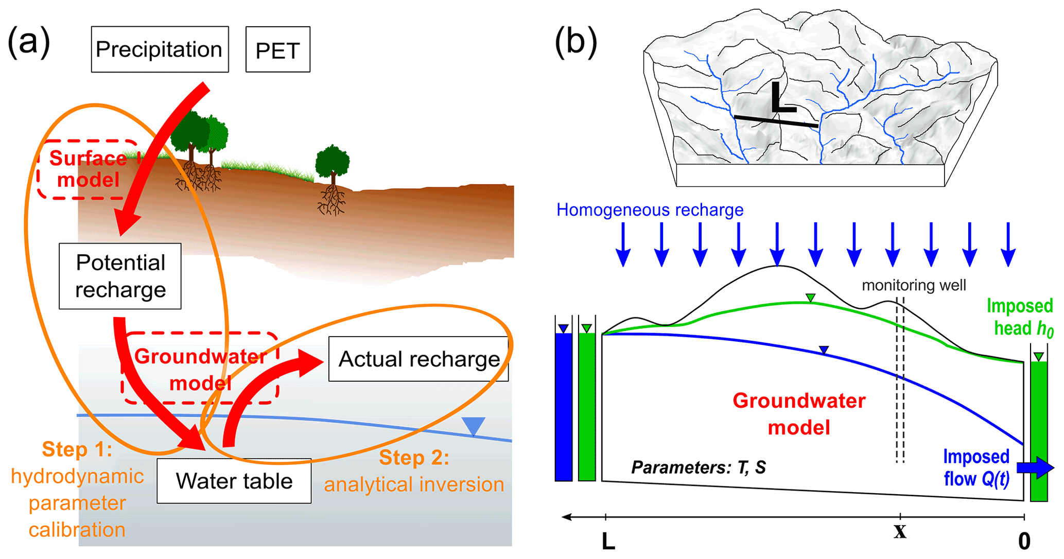
Figure 1 (a) Description of the method to estimate recharge from observed water table fluctuations. Step 1 infers groundwater model parameters using potential recharge estimates as input. Step 2 consists in estimating actual recharge from observed water table fluctuations using parameters (obtained from Step 1) in an analytical inversion. PET refers to potential evapotranspiration. (b) Description of the homogeneous 1D groundwater flow model. Recharge rate, R(t), is uniformly distributed along model length L. Model boundary conditions are a constant head at x=L and either a constant head or imposed flow rate at x=0 in order to represent natural (green case) and pumped systems (blue case). Note that the aquifer is assumed to be of uniform thickness with confined behavior under the Dupuit assumption so that the aquifer thickness does not matter in the model.

Recharge, as the main water inflow feeding GW, is critical for the proper management of GW systems. GW recharge is defined as the water percolating from the last unsaturated horizon down to the water table and is therefore broadly inaccessible to direct observations (Scanlon et al., 2006; Healy and Cook, 2002). It can be measured by a lysimeter or different tracing methods (Scanlon et al., 2002). Such methods are subject to spatial variability and difficult to upscale because recharge is spatially heterogeneous and controlled by multiple factors such as vegetation (Riedel and Weber, 2020; Perkins et al., 2014), soil properties (Kollet, 2009; Sililo and Tellam, 2000; Mohan et al., 2018) and hydrogeological conditions (Kollet and Maxwell, 2008; Fan et al., 2019; Appels et al., 2015).

Modeling the recharge is therefore a relevant method to estimate it. Several recharge models have been developed (Healy, 2010; Simunek et al., 2005), ranging from a fraction of annual precipitation to more complex land surface models resolving energy and water budgets from local to regional scale (Morton, 1983; Thornthwaite, 1948; Wada et al., 2010; Döll and Fiedler, 2008; Mohan et al., 2018; Hartmann et al., 2017). All of these studies assess the GW recharge “from above” (i.e., from the surface towards the aquifer). Such an approach is hampered by uncertainties in the estimation of surface fluxes (rainfall, evapotranspiration and runoff) (Long et al., 2014; Riedel and Weber, 2020), soil model structural errors, and hydrodynamic properties' variabilities and uncertainties (Hartmann et al., 2017; Lee et al., 2006; Nicolas et al., 2019). Moreover, this approach, where modeled soil thickness is limited to a few meters, does not consider the actual water table depth (Clark et al., 2017). We argue these estimates provide only “potential GW recharge” (Fig. 1) because of potential storage changes and lateral flow in the deep unsaturated zone (Besbes and Marsily, 1984; Cao et al., 2016).

Oppositely, GW recharge can also be estimated “from below”. GW levels in boreholes are indeed the most direct observation to characterize aquifers behavior. The water table fluctuation (WTF) method has thus been used to provide vertical recharge estimates from GW-level variations (Healy and Cook, 2002; Crosbie et al., 2005; Maréchal et al., 2006; Cuthbert, 2010; Cuthbert et al., 2016, 2019b; Labrecque et al., 2020). However, GW-level variations are also influenced by GW lateral flows, themselves depending on GW boundary conditions, making the estimation of the recharge from GW levels difficult. The main uncertainties arise from the limited knowledge on hydrodynamic parameters, such as specific yield, and the limitation of one observation point to infer flow characteristics in heterogeneous aquifers. Several authors therefore proposed to apply a frequency analysis between long-term data of recharge and GW levels assuming an equivalent homogeneous aquifer (Gelhar, 1974). In this case, time lags and amplitudes of aquifer response to periodic recharge can be described by a linear transfer function (Jimenez-Martinez et al., 2013; Townley, 1995). Based on this theoretical framework, Dickinson (2004) inverted the method to infer time-varying recharge linked to climate variability from GW levels. However, this method focuses on long-term periodic cycles.

While strong attention has been put on mean annual recharge estimations, the characterization of recharge fluctuations (RFs) over time, at short to long timescales, remains critical and has been investigated less. This has been highlighted as one of the 23 unsolved problems in hydrology (Blöschl et al., 2019). Recharge is highly variable throughout the year, showing a pronounced seasonality (Jasechko et al., 2014; Gabrielli and McDonnell, 2018) with potential high sensitivity to intense rainfall events (Taylor et al., 2012; Owor et al., 2009; Mileham et al., 2009). RFs are also modulated by water table depth, human actions such as pumping (Bredehoeft, 2002) or return flow from irrigation (Taylor et al., 2013; Guihéneuf et al., 2014; Le Coz et al., 2013). Several authors highlighted that changes in recharge impact groundwater flow. For example, irrigation and GW abstraction impact recharge and discharge variability in space and time (Cao et al., 2016; Lee et al., 2006; Shamsudduha et al., 2011; Johansen et al., 2011). Another example is that topographic control on GW flow depends on recharge (Bresciani et al., 2016; Marçais et al., 2017). Recently, several works also documented that modifications to surface or subsurface characteristics (soil properties, vegetation, etc.) would affect the hydrological response – including groundwater – at annual to interannual timescales (Ajami et al., 2017; Troch et al., 2009; Fan, 2015; Condon and Maxwell, 2017; Favreau et al., 2009).

In this study, we propose to quantify the RFs by developing a novel method able to quantify the GW recharge from below. The main objectives of this work are thus threefold: (1) deciphering the respective impact of GW lateral flow and recharge on GW-level fluctuations in heterogeneous aquifers, (2) estimating RFs over a 20-year period and (3) studying how rainfall distribution and unsaturated zone thickness controls GW recharge. To do that, we develop the WTF method in the frequency domain to decompose GW-level fluctuations into GW lateral flow and RFs (Sect. 1). While GW systems are heterogeneous in nature, we propose to represent them by an equivalent homogeneous 1D Dupuit model (Fig. 1). We apply this method on two fractured crystalline aquifers, one heavily pumped and one in a natural context. We also test the consistency of this newly developed method among the different observation wells of the two sites. For each well, we first estimate hydrodynamic parameters before inverting the model analytically to propose RF estimates. The GW model (Sect. 2) offers the advantage of requiring few parameters, running fast and adapting to different boundary conditions, as illustrated by the two application sites. Associated GW-level observations and prescribed potential recharge rates are presented in Sect. 3. Once the model reproduces GW-level fluctuations (Sect. 4), RFs can be inverted analytically (Sect. 5). Finally, RFs between the two sites are compared, and main results are discussed (Sect. 6).

2 Modeling approach: from water table to water transfer within the unsaturated zone

2.1 Main steps

The method developed in this study relies on several steps, as illustrated by Fig. 1. The initial step consists of providing a first estimate of potential groundwater recharge for the study area. These data are given at a daily time step. Then, the GW analytical model is defined as a function of the boundary conditions for each observation well of the study site. The next step consists in calibrating model parameters by comparing simulated WTFs to WTFs observed in boreholes (Step 1 in Fig. 1). The method allows the respective impact of GW lateral flow and recharge on WTFs to be deciphered. To achieve this goal, hydrodynamic parameters are calibrated by prescribing different sets of potential RFs. Then, the GW model is reversed analytically (Step 2 in Fig. 1) using calibrated parameters at each borehole with the aim to compute RFs from observed WTFs. While unsaturated zone thickness is not considered during Step 1 (potential recharge equals recharge), it is expected that Step 2 reveals its importance.

As developed below, we focus on water table and recharge anomalies, here called “fluctuations”. These fluctuations are obtained by removing the mean value from input data (potential recharge and pumping rates used during Step 1) over the study period. Consequently, simulated WTFs obtained during Step 1 will be compared to observed fluctuations. Finally, RFs are obtained from observed WTFs (Step 2) and will be compared to potential RFs.

In the next sections, we describe (1) the analytical GW flow model deployed to estimate recharge from observed WTFs, (2) the soil models used to estimate potential recharge as input to the GW model, (3) the GW parameter calibration strategy and (4) the analytically inverted GW model. Finally, we also present how inverted recharge is analyzed with rainfall at the two study sites.

2.2 Defining the 1D GW flow model for each field site

Considering a homogeneous and confined aquifer, and assuming that the vertical component of the GW flow can be neglected (Dupuit assumption), the GW flow equation can be described by a diffusion equation (Eq. 1) (De Marsily, 1986):

$$\begin{array}{}\text{(1)}& T{\displaystyle \frac{{\partial }^{\mathrm{2}}h(x,t)}{\partial x^{\mathrm{2}}}}=S{\displaystyle \frac{\partial h(x,t)}{\partial t}}-R\left(t\right),\end{array}$$

where h(x,t) denotes the hydraulic head variations [L], R(t) the uniformly distributed recharge rate from the surface [L T⁻¹], T the aquifer transmissivity [L² T⁻¹] and S the storage coefficient of the aquifer [–]. This formulation is also valid in unconfined aquifers if head variations are small compared to the aquifer thickness. In this case, S is equivalent to specific yield. The system is defined by a domain comprised between x=0 and x=L (Fig. 1).

Solving Eq. (1) requires two boundary conditions imposed at x=0 and x=L. In what follows, we consider a constant imposed head (h_L) at x=L and either an imposed flux (Q_pump(t)) or a constant imposed head (h₀) at x=0 depending on the site considered (the “pumping” site and the “natural” case respectively). These boundary conditions have been chosen to best represent actual aquifer configurations. The transient part of Eq. (1) with the associated boundary conditions can be solved analytically in the frequency domain (Townley, 1995; Carslaw and Jaeger, 1959), and this leads to Eq. (2) and (3) describing WTFs (h(x_r,t)). The derivation of these equations is provided in Appendix A.

$$\begin{array}{}\text{(2)}& {\displaystyle }\begin{array}{rl}h\left(x_r,t\right)& =\sum \mathrm{Re}\left\{e^{i\mathit{\omega }t}\left[{\displaystyle \frac{\stackrel{\mathrm{‾}}{R}\left(\mathit{\omega }\right)}{i\mathit{\omega }S}}\left(\mathrm{1}-{\displaystyle \frac{\cosh \left(x_r\sqrt{i\mathit{\omega }{t}_{\mathrm{c}}}\right)}{\cosh \left(\sqrt{i\mathit{\omega }{t}_{\mathrm{c}}}\right)}}\right)\right.\right.\\ & \left.\left.+{\displaystyle \frac{\stackrel{\mathrm{‾}}{Q}\left(\mathit{\omega }\right)}{W}}{\displaystyle \frac{L}{T\sqrt{i\mathit{\omega }{t}_{\mathrm{c}}}}}{\displaystyle \frac{\sinh \left(\sqrt{i\mathit{\omega }{t}_{\mathrm{c}}}\left(x_r-\mathrm{1}\right)\right)}{\cosh \left(\sqrt{i\mathit{\omega }{t}_{\mathrm{c}}}\right)}}\right]\right\}\\ & \left(\mathrm{pumping}\mathrm{site}\right)\end{array}\text{(3)}& {\displaystyle }\begin{array}{rl}h& \left(x_r,t\right)=\sum \mathrm{Re}\left\{e^{i\mathit{\omega }t}\left[{\displaystyle \frac{\stackrel{\mathrm{‾}}{R}\left(\mathit{\omega }\right)}{i\mathit{\omega }S}}\right.\right.\\ & \left.\left.\left(\mathrm{1}+{\displaystyle \frac{\sinh \left(\sqrt{i\mathit{\omega }{t}_{\mathrm{c}}}\left(x_r-\mathrm{1}\right)\right)-\sinh \left(x_r\sqrt{i\mathit{\omega }{t}_{\mathrm{c}}}\right)}{\sinh \left(\sqrt{i\mathit{\omega }{t}_{\mathrm{c}}}\right)}}\right)\right]\right\}\\ & \left(\mathrm{natural}\mathrm{site}\right),\end{array}\end{array}$$

$$\mathrm{with}D={\displaystyle \frac{T}{S}},X=\sqrt{{\displaystyle \frac{D}{i\mathit{\omega }}}},x_r={\displaystyle \frac{x}{L}},\mathrm{and}{t}_{\mathrm{c}}={\displaystyle \frac{L^{\mathrm{2}}}{D}}.$$

Equations (2) and (3) highlight the importance of characteristic time (t_c) (Domenico and Schwartz, 1998) describing how a pressure pulse is propagated along the distance L. Note that the pumping case requires input for model width W to define a volume per unit of time (see Fig. A1 and Appendix A2). While GW pumps are actually localized in boreholes, boundary conditions should be applied along the width W of the 1D model. Here, we consider a field site (Ploemeur) where pumping wells are concentrated within a “pumping zone” constituting the outlet of the system. Therefore, the propagation of the pumping through the aquifer is simulated in a physical way. The weak impact of the parameter W in estimating hydrodynamic parameters and recharge is assessed separately in the Supplement. In addition, the approach was also tested in radial coordinates to compare the impact of model geometry in the pumping case (Supplement). Several analytical solutions corresponding to different hydrogeological configurations are also provided in the attachment to this study. The analytical model is evaluated in Appendix B1 by comparing WTFs obtained from Eq. (3) to WTFs obtained from a numerical model with similar geometry and parameters.

Equations (2) and (3) describe WTFs as a function combining the Fourier transform of the recharge and the pumping ($\stackrel{\mathrm{‾}}{R}$ and $\stackrel{\mathrm{‾}}{Q}$) modulated by the transient events frequency (ω). Therefore, high frequencies contained in R(t) and Q(t) are dampened in WTFs as a function of t_c and (x_r) (the monitoring well relative position inside the domain; see Fig. 1b). For the pumping site, x_r corresponds to the distance to the pumping barycenter, defined as the geometric midpoint between the pumping wells weighted according to pumping rates. Note that these analytical solutions, corresponding to the transient state, do not depend on the constant head imposed at x=L and at x=0 for the natural case. Therefore, WTFs are not impacted by the mean hydraulic gradient, which constitutes a major advantage of our method by reducing the number of parameters and uncertainty on the input lateral flow at x=L (see Appendix C dealing with the steady part of Eq. 1).

2.3 Estimating potential recharge from above

The GW model described previously is driven by GW recharge R(t). In order to assess GW model sensitivity to prescribed recharge estimates, we tested three different classical soil models computing potential recharge from above (from the surface towards the aquifer as described in Fig. 1). These three potential recharge data differ in terms of mean value and time-dependent fluctuations. Soil models use daily climate data to infer daily potential recharge defined as percolation below the root zone. We consider that potential recharge is instantaneously input to the GW system as actual recharge, thereby neglecting unsaturated zone processes between the modeled soil layer and the actual water table depth. To focus on the temporal fluctuations and avoid the issues related to the steady part (see Appendix C), we subtract the mean value from the modeled potential recharge data before providing them to the GW analytical model.

The first – and simplest – soil model, called “Thornthwaite”, is based on the representation of the unsaturated zone as a simple reservoir accumulating rainwater and satisfying potential evapotranspiration (calculated using the Thornthwaite method) while water is available. When the reservoir is full, excess water recharges GW (Thornthwaite, 1948). Such a model neglects surface runoff. In Brittany, surface runoff is expected to be relatively low for most of the year due to moderate rain intensities, lack of high reliefs, and steep slopes and vegetation that favor infiltration. Based on previous studies at the Ploemeur site (Jimenez-Martinez et al., 2013), we consider a soil storage reserve of 166 mm based on a local soil characterization.

The second soil model is derived from the GR4J hydrological model (Perrin et al., 2003). Potential recharge estimates are based on the so-called production store and defined as the sum of downward fluxes from the production store (see https://webgr.irstea.fr/modeles/journalier-gr4j-2/, last access: 15 April 2022). In this model, evapotranspiration and other water fluxes depend on the amount of water stored in the reservoir in a nonlinear but incremental way, providing more diffuse infiltration as compared to the previous model. After several tests, the capacity of the production store is set to 300 mm in order to provide more recharge with a more diffuse behavior compared to the Thornthwaite model.

The third potential recharge estimate is provided by the SURFEX modeling platform. SURFEX is composed of a spatially distributed land surface model (Interaction between Soil Biosphere and Atmosphere, ISBA) that simulates water and energy fluxes at the interface between the atmosphere and the surface (soil, vegetation and snow) (Noilhan and Planton, 1989; Masson et al., 2013). SURFEX is provided on a 8 km grid over France. Potential recharge corresponds to the water drained below the root zone, also called “deep drainage”.

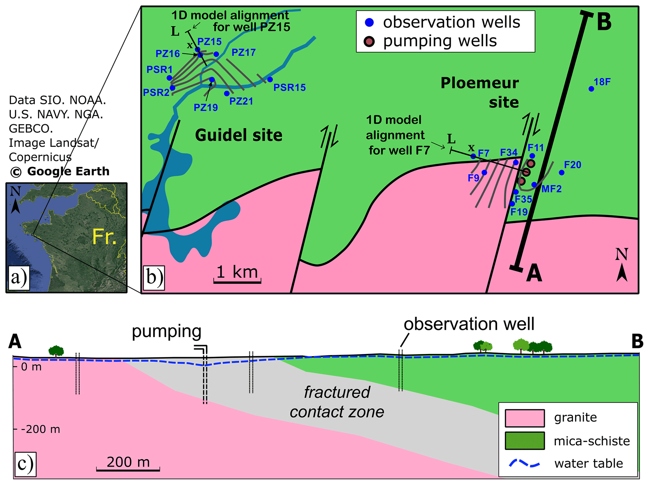
Figure 2 Schematic of Ploemeur and Guidel sites. (a) Field sites location in France. (b) Geological map and location of monitoring (blue points) and pumping wells (red points) (modified from Ruelleu et al., 2010). Mean GW level measured over the piezometric network is represented by gray equipotential lines. For each site, one 1D model is illustrated by a black line. (c) South–north cross section of the Ploemeur site. Wells are generally screened over depths ranging from 30 to 100 m. Dashed blue line represents groundwater level.

2.4 GW model parameter calibration

The forward model is now fully defined. The first step of our approach consists in defining geometric (L and W) and hydrodynamic (T and S) parameters based on the comparison with measured groundwater levels. In the pumping case, W was chosen arbitrarily to be W=1000 m as a first parameter set exploration showed that this parameter did not influence results as long as W>500 m (Supplement). W does not appear in the analytical solution of the natural case. The location x of the observation wells also needs to be defined consistently with the 1D framework. In the pumping case, x is defined as the distance between the observation well and the pumping wells. In the natural case, x is defined as the distance to the nearest river (lower-boundary condition). Two examples of model alignment are illustrated in Fig. 2.

In order to explore the informative content of the observed WTFs to define geometric and hydrodynamic parameters, our strategy consists in defining equiprobable parameter sets testing sensitivity to imposed recharge rates (Sect. 2.3). Analytical GW models are computationally efficient. Thus, the whole parameter space (T, S and L) has been regularly sampled (in a logarithmic scale for T and S) inside a plausible range defined by values reported in comparable geological settings of Brittany and beyond: transmissivity $T\in [{\mathrm{10}}^{-\mathrm{4}}$; $\mathrm{2}\times {\mathrm{10}}^{-\mathrm{1}}]$ m² s⁻¹ (40 values), storage coefficient $S\in [{\mathrm{10}}^{-\mathrm{4}}$; $\mathrm{2}\times {\mathrm{10}}^{-\mathrm{1}}]$ (40 values) and length L∈[800; 6000] m (53 values). We refer to Le Borgne et al. (2006) and Leray et al. (2014) regarding hydrodynamic properties expected at the Ploemeur site. Regarding the storage coefficient, a 0.01–0.2 range can be considered to reflect weathered and fissured horizons (see Kovacs, 1981; Wright and Burgess, 1992; Singhal and Gupta, 2010, for values in shallow weathered zones, and Earle, 2015; Hiscock, 2009, for granites and schists). Regarding length L, we refer to the density of the river network in the region. In Brittany, the hillslope length is typically 1 km (Lague et al., 2000). For the Guidel site, length L varies between 20 and 2000 m with 100 values. This range is smaller than for Ploemeur site because L is expected to be smaller in “natural conditions” compared to pumping conditions where water table drawdown tends to extend the system (Fig. 1). In addition, three sets of potential recharge rates have been imposed on the Ploemeur site model. So, a total of 254 400 and 160 000 simulations were run for each monitoring well for Ploemeur and Guidel sites respectively. This approach allows for estimation of the extent to which model parameters can be defined with observed WTFs. In order to reduce computing time during model calibration, the model is run at a 7 d time step.

For each observation well, modeled WTFs are evaluated against root mean square error (RMSE) divided by the standard deviation of observed WTFs (called normalized RMSE, nRMSE) to favor comparison among the different observation wells:

$$\begin{array}{}\text{(4)}& \mathrm{nRMSE}=\sqrt{{\displaystyle \frac{\sum {\left(h_{\mathrm{obs}}-h_{\mathrm{model}}\right)}^{\mathrm{2}}}{n}}}\times {\displaystyle \frac{\mathrm{1}}{{\mathit{\sigma }}_{\mathrm{obs}}}},\end{array}$$

where n is the number of samples, and σ_obs is the standard deviation of observed data. In addition, we assessed the model performance by comparing parameter estimates and simulated water table when calibration is based on the first half of the observation period (see calibration–validation in the Supplement).

2.5 From WTFs to recharge: analytical inversion or backward model

In a last step, GW recharge (R(t)) is analytically determined from Eq. (2) for the pumping case. Indeed, when hydrodynamic parameters (Sect. 2.4) and boundary conditions (Q(t)) are known, WTFs (h_obs(x,t)) can be reversed analytically (Appendix A3) in the frequency domain in order to infer the Fourier transform of recharge (Eq. 5):

$$\begin{array}{}\text{(5)}& \begin{array}{rl}\stackrel{\mathrm{‾}}{R}\left(\mathit{\omega }\right)& =\left(i\mathit{\omega }S\stackrel{\mathrm{‾}}{h}\left(x_r,\mathit{\omega }\right)-{\displaystyle \frac{\stackrel{\mathrm{‾}}{Q}\left(\mathit{\omega }\right)}{W}}{\displaystyle \frac{\sqrt{i\mathit{\omega }{t}_{\mathrm{c}}}}{L}}{\displaystyle \frac{\sinh \left(\sqrt{i\mathit{\omega }{t}_{\mathrm{c}}}\left(x_r-\mathrm{1}\right)\right)}{\cosh \left(\sqrt{i\mathit{\omega }{t}_{\mathrm{c}}}\right)}}\right)\\ & \times {\left(\mathrm{1}-{\displaystyle \frac{\cosh \left(x_r\sqrt{i\mathit{\omega }{t}_{\mathrm{c}}}\right)}{\cosh \left(\sqrt{i\mathit{\omega }{t}_{\mathrm{c}}}\right)}}\right)}^{-\mathrm{1}}.\end{array}\end{array}$$

$\stackrel{\mathrm{‾}}{R}\left(\mathit{\omega }\right)$ appears expressed as an equivalent water layer ($S\cdot \stackrel{\mathrm{‾}}{h}$) minus the impact of pumping $\stackrel{\mathrm{‾}}{Q}/\left(WL\right)$ redistributed on the system by a space–time function (sine and cosine hyperbolic functions). Finally, the monitoring well position ($x_r=x/L$) also plays an important role when estimating recharge from observed GW levels as GW-level variations integrate both vertical and lateral recharge. Note that backward models are run at a daily time step to benefit from the observed WTFs and because backward models are run only with a set of best parameters (Sect. 2.4).

A similar analytical solution is obtained for the case without pumping from Eq. (3), as described by Eq. (6).

$$\begin{array}{}\text{(6)}& \begin{array}{rl}\stackrel{\mathrm{‾}}{R}\left(\mathit{\omega }\right)=& i\mathit{\omega }S\stackrel{\mathrm{‾}}{h}\left(x_r,\mathit{\omega }\right)\\ & {\left(\mathrm{1}+{\displaystyle \frac{\sinh \left(\sqrt{i\mathit{\omega }{t}_{\mathrm{c}}}\left(x_r-\mathrm{1}\right)\right)-\sinh \left(x_r\sqrt{i\mathit{\omega }{t}_{\mathrm{c}}}\right)}{\sinh \left(\sqrt{i\mathit{\omega }{t}_{\mathrm{c}}}\right)}}\right)}^{-\mathrm{1}}\end{array}\end{array}$$

Then, RFs are computed by the inverse Fourier transform. RF uncertainties are evaluated by propagating parameter uncertainties. Thus, for both cases, RFs can be estimated from WTFs taking into account lateral flow and unsaturated zone influence in contrast to the classical method computing recharge from above (described in Sect. 2.3).

This new approach has been evaluated with a numerical MODFLOW model (see Appendix B). The evaluation consists of providing daily recharge rates (Thornthwaite model) to a numerical model equivalent to the analytical 1D model used for the Guidel case. The resulting WTFs at x_r=0.75 are then used in Eq. (6) to estimate RFs. Similar RF estimates would lend support for the analytical approach. We found that analytically estimated RFs are similar at the 1 % level to the reference Thornthwaite RFs integrated over 10 d time steps. Thus, the analytical model allows RFs to be estimated accurately on an ideally designed site (known parameters and simple 1D geometry). This numerical test also brings first insights on the impact of parameters uncertainty on estimated recharge: a factor 2 uncertainty in storativity S directly corresponds to a factor 2 uncertainty in recharge volumes, considering other parameters are fixed, while uncertainty on characteristic time is less pronounced.

2.6 How unsaturated zone transforms precipitation into recharge

Finally, rainfall fluctuations obtained from climate data and RFs obtained by inverting the best GW models are analyzed at both sites in time and frequency domains. The classical approach consists in defining statistics on the distribution and intensity (e.g., number of days without rain, cumulative sorted rainfall) but does not often yield satisfactory results. Considering the relationship between P−PET and recharge as a frequency-dependent function is a simple but effective way to consider the impact of rainfall distribution on recharge. This function defines the relative efficiency to generate recharge between a single rainfall event and a long-lasting wet season and has been recently tested by Schuite et al. (2019).

In order to focus on the transformation of rainfall into recharge, we compute both the coherence and the transfer function (Jimenez-Martinez et al., 2013) between recharge and rainfall minus potential evapotranspiration, P−PET (also expressed as variations with respect to the long-term mean). The coherence C_XY(ω) examines the relationship between two signals X(t) (P−PET fluctuations) and Y(t) (recharge fluctuations) by computing the frequency-dependent correlation, defined as

$$\begin{array}{}\text{(7)}& C_{XY}\left(\mathit{\omega }\right)={\displaystyle \frac{P_{XY}(\mathit{\omega }{)}^{\mathrm{2}}}{P_{XX}\left(\mathit{\omega }\right)P_{YY}\left(\mathit{\omega }\right)}},\end{array}$$

where P_XY(ω) is the cross-spectral density between X(t) and Y(t), and P_XX(ω) and P_YY(ω) are the autospectral density of X(t) and Y(t) respectively. The transfer function $\stackrel{\mathrm{‾}}{H}\left(\mathit{\omega }\right)$ describes the amplitude ratio between output and input in the frequency domain as

$$\begin{array}{}\text{(8)}& \stackrel{\mathrm{‾}}{Y}\left(\mathit{\omega }\right)=\stackrel{\mathrm{‾}}{H}\left(\mathit{\omega }\right)\stackrel{\mathrm{‾}}{X}\left(\mathit{\omega }\right).\end{array}$$

Thus, the transfer function quantifies P−PET efficiency to recharge GW, i.e., a proxy of rainfall efficiency. These transfer functions comparing flux coming in vs out of the unsaturated zone allow its role in the recharge dynamics to be inferred. Switching to the frequency domain offers the additional advantage to visualize how precipitation is converted into recharge at each frequency. As a comparison, we also computed coherence and transfer functions between P−PET and potential recharge. Here, we used “mscohere” and “tfestimate” MATLAB functions. Coherence and transfer function are computed by dividing overlapping sections of 280 d, windowed by a Hamming function, and overlapping them by 50 %.

3 Application sites and data

3.1 The Ploemeur and Guidel observatories

The model ability to estimate RFs is tested on the Ploemeur–Guidel hydrogeological observatory (http://hplus.ore.fr/en/ploemeur, last access: 4 May 2022), a part of the H⁺ network (http://hplus.ore.fr/en/, last access: 4 May 2022) and the French Critical Zone network OZCAR (http://ozcar-ri.org/, last access: 4 May 2022) (Gaillardet et al., 2018). Neighboring sites (Fig. 2) are set in a similar climatic, geologic and land cover context. The landscape consists of fields and meadows with slight topography (average slope around 3 %). GW is hosted in highly fractured crystalline rocks (Ruelleu et al., 2010; Touchard, 1999; Jimenez-Martinez et al., 2013). The Ploemeur site has been pumped since 1991, while the Guidel site has not been perturbed by pumping and hosts large GW upflowing zones, creating groundwater-dependent ecosystems.

Crystalline rocks are generally considered impermeable. However, several examples show high-yielding aquifers, which are mostly explained by the presence of fractures and weathered porous structures (Roques et al., 2016; Bense et al., 2013; Wyns et al., 2004). The Ploemeur site is a striking example as the site has been producing more than 1×10⁶ m³ yr⁻¹ of water since 1991. The high yield of the Ploemeur aquifer is explained by the presence of a contact zone between granite and mica schist, which is highly fractured and gently dipping towards north (Fig. 2). Such structures are preferential pathways for water, which also allow for drainage of a wide region beyond the topographic catchment (Ruelleu et al., 2010; Touchard, 1999; Leray et al., 2012; Jimenez-Martinez et al., 2013). The thickness of the weathered zone varies from 0 to 30 m. Several studies highlighted the heterogeneity within the Ploemeur observatory through borehole experiments (Le Borgne et al., 2006, 2007; Dewandel et al., 2014) or water chemistry monitoring (Roques et al., 2018). Local investigations at the borehole scale also show that deep fractures can be well connected with surface. For instance, recent temperature monitoring suggests that deep fractures (80 m deep) may be very sensitive to recharge (Pouladi et al., 2021).

At the Ploemeur site, more than 25 wells have been monitoring groundwater levels since 1991. These wells are generally ∼100 m deep and screened over depths ranging from [30–100] m. As these wells are mostly localized in the vicinity of the pumping site (at a distance < 700 m), i.e., close to the aquifer outflow, they provide a partial view on the aquifer behavior (Roques et al., 2018). GW is extracted by three pumping wells close to the contact between mica schist and granite (north of the southern granitic outcrop) (Fig. 2). The three pumping wells are aligned along a N20^∘E direction and spaced out by around 50 m (Fig. 2). Pumping rates were measured weekly from 1991 to 1997, daily since 1997 and hourly since 2015. Mean GW abstraction stabilized at 3000 m³ d⁻¹, with a seasonal variability around 15 % due to local demand increase during summer. Pumping creates a radial flow structure over a few hundreds of meters, stretched along the N20^∘E direction, and induces a unsaturated zone thickness of ∼15 m on average on the well network. Flow structure becomes unidirectional (1D) over the remaining system (∼2–3 km long) (Leray et al., 2012), so that flow convergence can be neglected at aquifer scale (Fig. 2). Therefore, the 1D assumption required by the analytical model can be valid at the hydrogeological system scale (Fig. 2).

The Guidel site (Bochet et al., 2020) is located 4 km west of the Ploemeur site (Fig. 2) in the same geological context. GW levels are much closer to the surface, especially in convergence zones (downstream borehole PZ19), so that hydraulic gradients are more controlled by topography. The unsaturated zone thickness is ∼4.5 m on average on the well network. GW discharges to rivers and a wetland (Fig. 2).

3.2 Model setup

Conceptually, each monitoring well intercepts a flow line between two distant boundary conditions. For the pumping site (Ploemeur site), the coordinate x of each monitoring well corresponds to its actual distance to the pumping barycenter. At x=0, we impose transient pumping rates based on recorded pumping data. At x=L, we assume a constant hydraulic head (blue case in Fig. 1), typically representing the nearest river in that direction. Thus, the upstream area of the pumping is not fixed.

For the natural case study (Guidel site), each monitoring well is part of one hillslope bounded by a river at x=0 and bounded by another hillslope at x=L. So, the boundary condition in x=L should be a no flow condition. But similar to Ploemeur, we considered a constant head at x=L, corresponding to another hillslope boundary. Thus, $x=L/\mathrm{2}$ would correspond more or less to the watershed divide between two hillslopes. This condition allows the watershed divide to move along x seasonally. Here, the river level is shallow (typically 10–50 cm) and conceptually represents a constant head, as suggested by limited WTFs observed at borehole PZ19 close to the river (Fig. 3). In such a context, the assumption of an imposed constant head at x=0 is reasonable (boundary conditions colored in green in Fig. 1).

Figure 3 Observed GW-level variations in boreholes at the Ploemeur pumping site (a) and the Guidel natural site (b). Note the difference in scales between the two sites. m a.s.l. refers to meters above sea level.

3.3 Groundwater-level data

While first GW-level data at Ploemeur date back to 1991, we focus our analysis on the 1996–2017 period to avoid potential transient responses to the pumping setup. At the Guidel site, data are available from 2009 to 2017. Water levels are recorded at minute to daily time steps and decimated to daily timescales for our analysis. Hydraulic heads measured in boreholes are corrected from atmospheric pressure variations.

In Ploemeur, GW levels are relatively deep due to the pumping (depth ∼7 to 30 m; see Fig. C1) but still contain seasonal and interannual variability (Fig. 3) due to both pumping and climate variations. Note that WTFs in Ploemeur boreholes have quite similar patterns. Seasonal variations decrease with the distance to the pump: the amplitude is 5 m at well F11, 2.5 m at F7 and 1 m at 18F, respectively, at a distance of ∼20, 700 and 1000 m from pumping wells.

Conversely, transient variations in response to the rainfall and water cycle vary significantly among boreholes in Guidel (lower graph in Fig. 3). WTFs are fairly stable for low-elevation wells located close to the GW outflow (PZ19 and PZ21). Conversely, monitoring wells located at the top of basin (PSR1, PSR2, PZ15, PZ16 and PZ17) exhibit larger seasonal variability – but still smaller than in a pumped context.

3.4 Climate data

A national weather station (METEO-FRANCE) is located in between the two study sites. It provides daily precipitation and Penman–Monteith potential evapotranspiration (PET) estimates. Both are used to generate potential recharge from Thornthwaite and GR4J soil models (next section), while climate data used by SURFEX are derived from large-scale climate simulations. Within the studied period (1996–2017), annual precipitation ranges from 600 to 1100 mm yr⁻¹ (mean of 880 mm yr⁻¹), with limited variability (standard deviation of 120 mm yr⁻¹). Rainfall has a low seasonal variability, even if 45 % of rainfall occurs between October and January. PET ranges from 670 to 890 mm yr⁻¹, with a mean of 760 mm yr⁻¹ with lower variability (standard deviation of 50 mm yr⁻¹). PET has a strong seasonal variability, with mean values going from 0.6 mm d⁻¹ in December and January to 3.6 mm d⁻¹ in June and July.

3.5 Potential recharge estimates

Within the studied period, mean potential recharge rates derived from Thornthwaite, GR4J and SURFEX models are respectively 242, 320 and 246 mm yr⁻¹, i.e., 28 %, 37 % and 28 % of rainfall (Fig. 4). Thus, Thornthwaite and SURFEX models provide similar annual amplitudes, while the amplitude is 30 % higher on average for GR4J. Such values are typical of Brittany given the precipitation rate and climate (Martin et al., 2006; Leray et al., 2012, 2014; Molénat et al., 1999). For the Thornthwaite model, the annual potential recharge rate ranges from 0 mm yr⁻¹ in 2002 to 600 mm yr⁻¹ in 2001, representing 0 % to 50 % of annual rainfall.

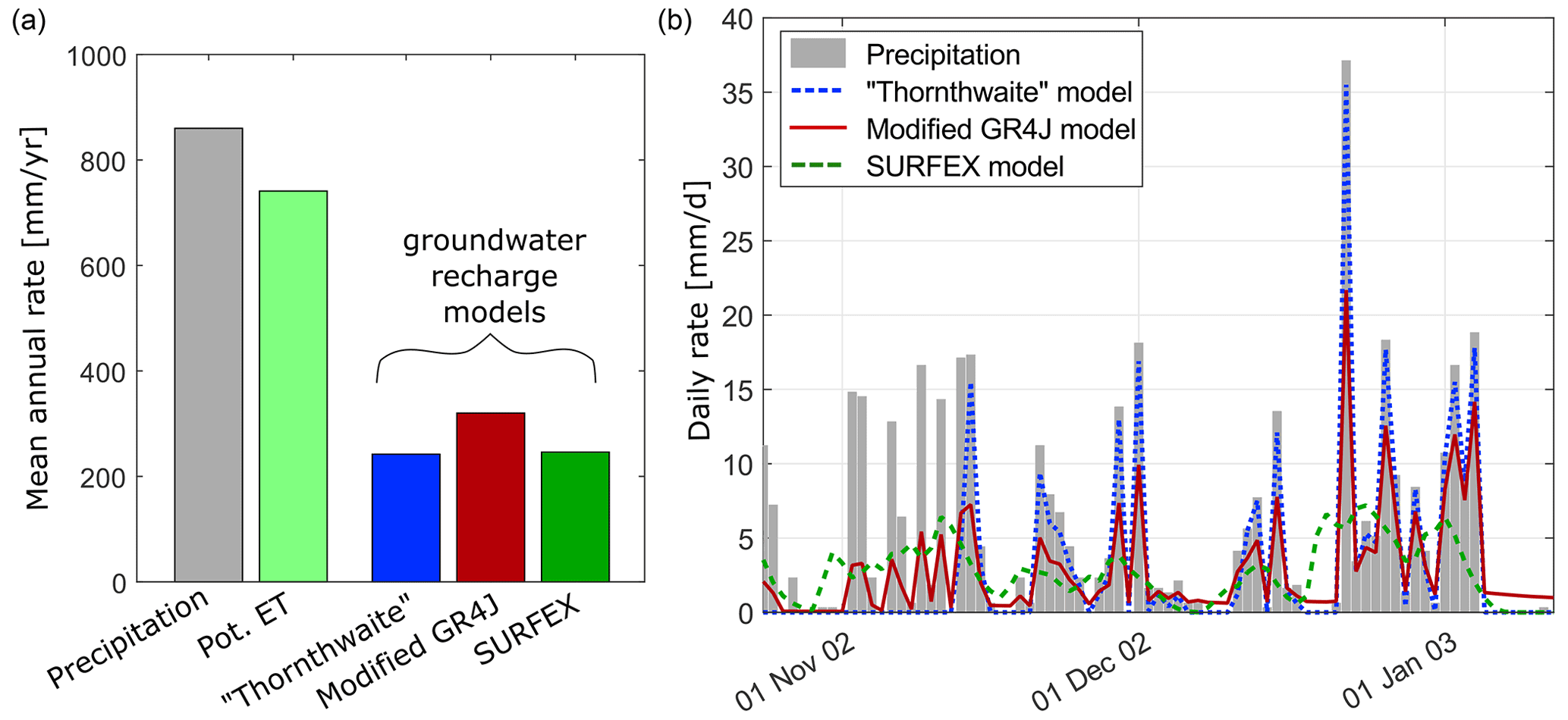
Figure 4 (a) Mean annual precipitation, potential evapotranspiration rate and estimated potential recharge rates from Thornthwaite, GR4J and SURFEX models on Ploemeur–Guidel sites (1996–2017). (b) Estimated daily potential recharge rates from Thornthwaite, GR4J and SURFEX models from November 2002 to January 2003. Daily precipitation (gray shaded bars) is recorded by a METEO-FRANCE weather station and is used to derive recharge from Thornthwaite and GR4J models.

Recharge typically occurs from December to March. Modeled potential recharge rates, as simulated by three different soil models, remain highly variable (Fig. 4). The Thornthwaite model (in blue in Fig. 4) generates episodic potential recharge events resulting from high-intensity rainfall. Daily events are on average more intense for the Thornthwaite model compared to GR4J (31 % smaller) and SURFEX (40 % smaller). GR4J- and SURFEX-modeled potential recharge events are more diffuse, with earlier events in late autumn (October–November) associated with high rainfall rates. The GR4J model also generates episodic recharge events in the summer period, linked to high rainfall intensity (summer storms).

4 Results

This section describes results obtained by applying and calibrating the 1D GW model to the two study sites (Step 1 in Fig. 1). We only focus here on water table fluctuations. The steady-state part of Eq. (1) (developed in Appendix A1 and A2) is described in Appendix C.

4.1 Modeling WTFs across the parameter set

This part synthesizes results of the parameter space exploration for the Ploemeur and Guidel sites. Observed and modeled WTFs are compared at different boreholes (see borehole locations in Fig. 2b).

4.1.1 Modeling WTFs with pumping conditions: Ploemeur site

Overall, the 1D GW model seems satisfactory when comparing observed and best modeled WTFs for the Ploemeur site (Fig. 5), whatever the imposed RFs. Corresponding model parameters, as well as impact of imposed recharge model, are described in the next section and illustrated in Fig. 6. For well F9, RMSE criteria are lower than 0.8 m, i.e., a factor 2.5 better than standard deviation of observed WTFs in this well (it corresponds to nRMSE of 0.4). While some wet or dry years are less well represented, seasonal to interannual variability is well modeled for all wells along the study period.

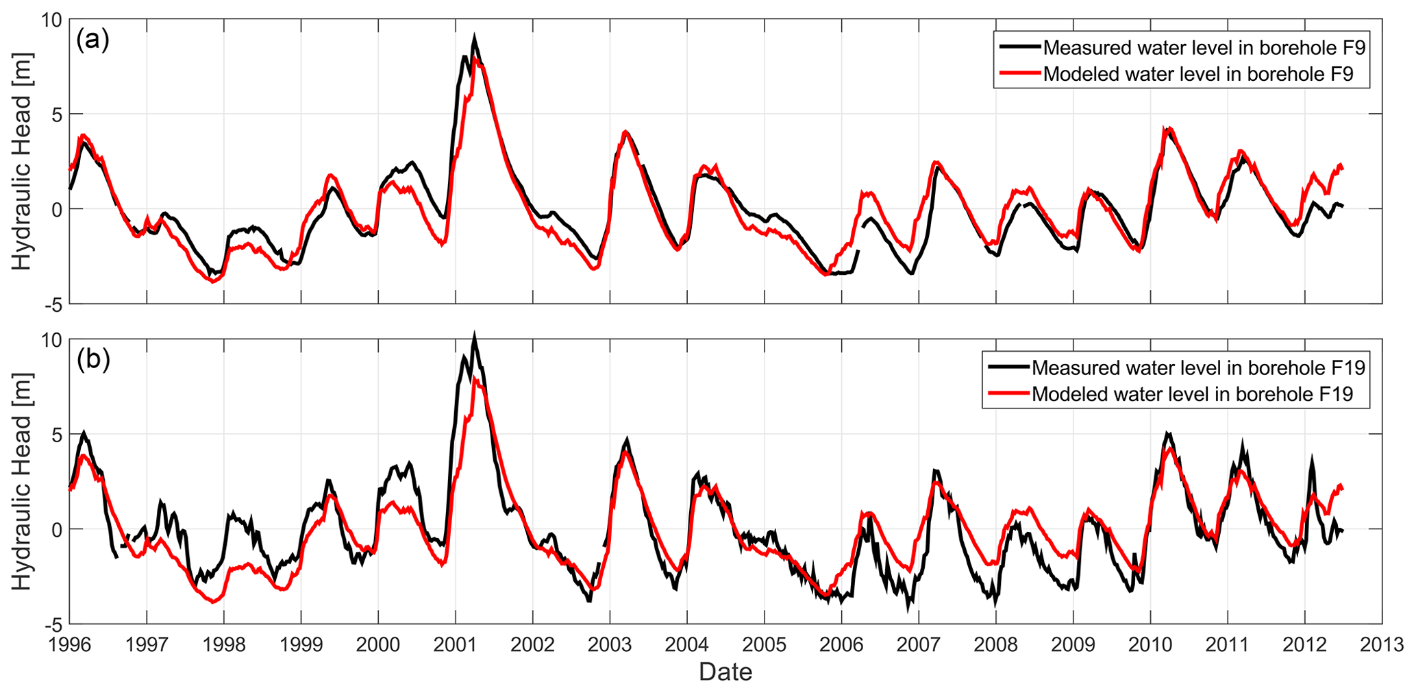
Figure 5 Comparison between best modeled and observed water table fluctuations at borehole F9 (a) and F19 (b), respectively at 519 and 268 m of Ploemeur's pumping wells. Hydraulic parameters correspond to best parameters (lowest RMSE in Fig. 6 regarding water table fluctuations). Prescribed recharge fluctuations have a negligible impact on these parameters and the quality of the fit.

The best RMSE for each borehole is increasing with decreasing distance to the pumping zone: ∼0.5 m at well F7, 0.7 m at F9, 1 m at MF2 and up to 1.2 m for well F11, which is 20 m away from the main pumping well. High-frequency fluctuations linked to daily to weekly pumping rate variations are not well described (see WTFs at F19 in Fig. 5). Such a result is explained by a lack of accurate pumping data. It also highlights that the GW model fails to simultaneously reproduce short timescale fluctuations driven by pumping and seasonal to annual fluctuations.

4.1.2 GW parameter sensitivity analysis

All parameters are not equally well determined (Fig. 6). For some parameters, the relation between model performance and parameter value shows a unique minimum, indicating that the parameter is constrained by observed WTFs. Characteristic time, storage coefficient and also transmissivity to model length ratio appear well constrained and quite similar between the different boreholes. For each borehole, we estimate parameter uncertainties by computing the model performance on WTFs (nRMSE) and fitting a normal distribution to the curves presented in Fig. 6. Optimal parameters and uncertainty are defined as the mean and standard deviation of this normal distribution.

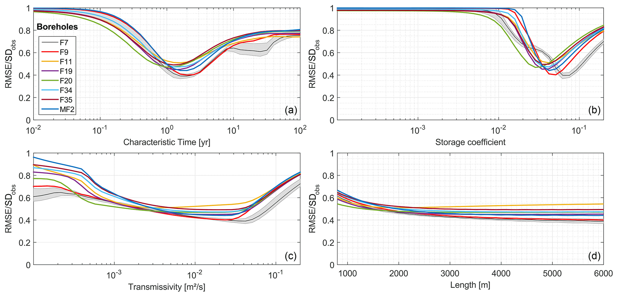
Figure 6 Evolution of the minimal normalized RMSE for Ploemeur wells as a function of model parameters: storage coefficient (b), transmissivity (c) and aquifer length (d). Evolution of characteristic time, a combination of the three parameters, is plotted in (a). We selected the best prescribed potential recharge model for each point. The impact of the prescribed recharge is shown by the shaded area on borehole F7.

Interestingly, storativity is well constrained as $S\in [\mathrm{2}\times {\mathrm{10}}^{-\mathrm{2}}$; $\mathrm{1.3}\times {\mathrm{10}}^{-\mathrm{1}}]$ with a mean value of $\mathrm{5}\times {\mathrm{10}}^{-\mathrm{2}}$ (see top right of Fig. 6). S varies slightly among the different wells. The analytical solution (Eq. 2) shows that S participates in the overall amplitude of the well reaction to recharge, linked to recharge volume for each frequency. Storativity is slightly affected by uncertainties in prescribed recharge volumes. This is highlighted at borehole F7 (black line) in Fig. 6: the variability induced by the choice of the prescribed potential recharge model (gray shaded area) is very limited. Conversely, transmissivity and aquifer length are poorly estimated.

Estimated characteristic time, a combination of the three calibration parameters (Eq. 2), is well constrained and equal to 1.5 years. Values range between 0.3 and 7.6 years among different boreholes (top left in Fig. 6). Optimal values range from 1–2 years among different boreholes. These results suggest the parameter identifiability would benefit from replacing the aquifer length as a fitting parameter by the characteristic time. It could be achieved by reorganizing Eq. (2). However, this approach would not reduce the number of calibration parameters and requires more sampling as the characteristic time range is larger than length range. As for storativity, characteristic time estimation appears independent of prescribed potential recharge. Thus, recharge volume uncertainty (Fig. 4) has a limited impact on parameter estimation.

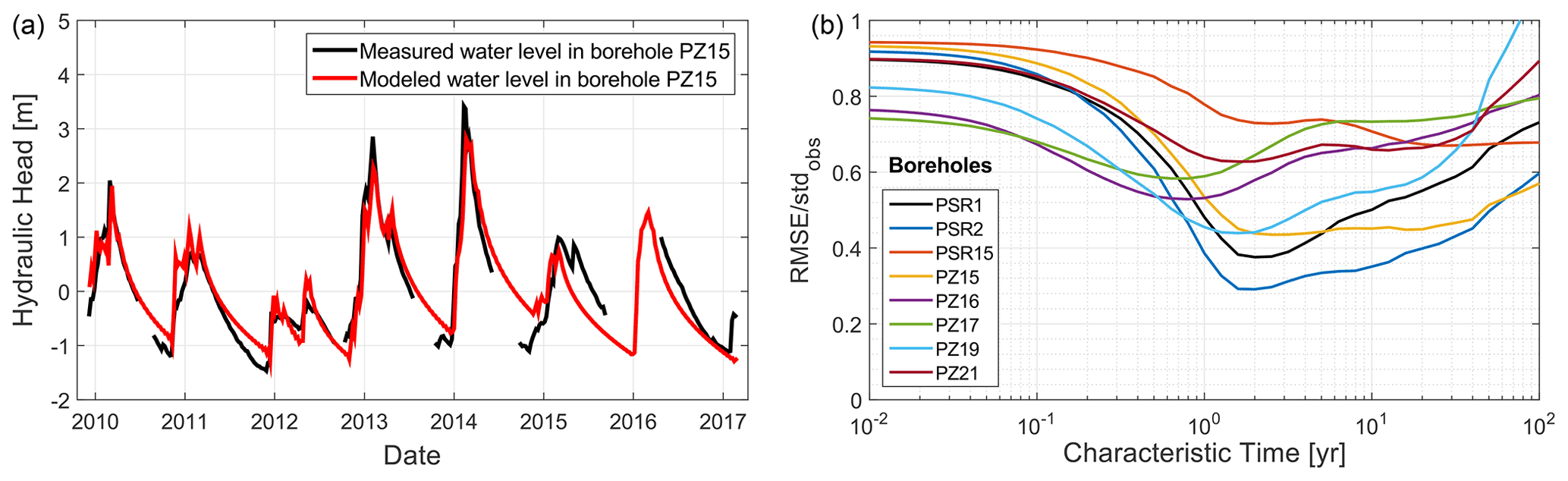
Figure 7 (a) Comparison between best modeled and observed water table fluctuations at borehole PZ15 in Guidel. Hydraulic parameters correspond to best parameters (lowest RMSE regarding water table fluctuations). (b) Evolution of the minimal normalized RMSE as a function of characteristic time, which is a combination of three parameters (storage coefficient, transmissivity and aquifer length), for Guidel boreholes.

4.1.3 Results and sensitivity analysis for Guidel site

Similarly to Ploemeur, the analytical GW model manages to adequately describe WTFs at Guidel (Fig. 7), although WTF patterns are very different (Fig. 3). Note we used the same potential recharge from Thornthwaite as in Ploemeur. For well PZ15, RMSE is 0.4 m, i.e., ∼40 % of the standard deviation of observed fluctuations. More generally, the model explains 40 % to 60 % of the WTF variability (right graph in Fig. 7), with RMSE around 0.4 m for wells located upstream, while it is limited to 0.1–0.2 m for wells located near the lower-boundary condition (PSR15, PZ19 and PZ21). Overall, model performance is slightly lower at Guidel than at the Ploemeur site. Therefore, model parameters are also less constrained. Characteristic times are close to those obtained at Ploemeur but with a wider range of 0.3–50 years (Fig. 7). The estimated storage coefficient ranges from $\mathrm{3}\times {\mathrm{10}}^{-\mathrm{2}}$ to $\mathrm{1.5}\times {\mathrm{10}}^{-\mathrm{1}}$ and transmissivity from 10⁻⁴ to $\mathrm{5}\times {\mathrm{10}}^{-\mathrm{3}}$ m² s⁻¹. Aquifer length is poorly defined and closely linked to transmissivity, as for the Ploemeur site.

5 Recharge fluctuation estimate from observed WTFs

5.1 Summary of the parameter space exploration

In the previous section, we showed that a simple GW model that neglects aquifer heterogeneity can reproduce observed WTFs well. An important result is that estimated hydrodynamic and geometric parameters are independent of prescribed potential recharge models (Fig. 4). They also appears quite independent of individual WTFs (Fig. 6). These parameters define lateral GW flow. So, the model can be further exploited to infer recharge from WTFs observed in different boreholes. For each borehole, RFs are estimated using parameter values from the 5 % best models.

Note that transmissivity is not well defined from temporal fluctuations. Mean water table in each borehole is impacted by heterogeneity (Fig. C1). As a consequence, mean (long-term) recharge cannot be accurately computed (see the steady-state term in Eq. A8). However, RFs, defined as recharge variations (or anomalies) with respect to the long-term mean, are fully reachable. In addition, even if parameter uncertainties can strongly impact the range of RF estimates (Appendix B), aquifer parameters (T, S and L) compensate for each other through model calibration such that characteristic time remains the most important parameter. Since characteristic time is obtained with a small uncertainty, its uncertainty has little impact on RF estimates (Appendix B).

5.2 Recharge fluctuation estimate for Ploemeur and Guidel sites

The analytical GW model appears as a low-pass filter in Eqs. (2) and (3), smoothing out high-frequency pumping and recharge variability (these variables are divided by frequency in Eqs. (2) and (3)). When computing recharge from the backward model (Eqs. 5 and 6), high-frequency WTF variability is amplified ($\stackrel{\mathrm{‾}}{h}$ is multiplied by frequency in Eqs. 5 and 6). Thus, noise linked to observation uncertainties in WTFs is amplified. The high-frequency (daily to monthly) variations of recharge increase when the borehole is well connected to the pumped fractured zone, as suggested by the difference in RFs between F9 and F19 (Supplement), 519 and 268 m away from the pumping station, respectively. This can be expected as observed WTFs contain high-frequency variations (Fig. 5) linked to short-term pumping rate variations (and the associated relative contribution of each pumping well), which are difficult to model. It only impacts high-frequency variations for some boreholes. This noise disappears when aggregating RFs at a monthly timescale.

Figure 8 shows analytically estimated RFs at a monthly scale for both Ploemeur and Guidel sites, including uncertainties linked to parameter uncertainty and observation well variability. Phase and amplitude of RFs are quite similar between the different wells, as illustrated by shaded areas. They are also similar at both sites, as illustrated by the overlapping of red and blue lines in Fig. 8, although WTFs are very different at each site (Fig. 3).

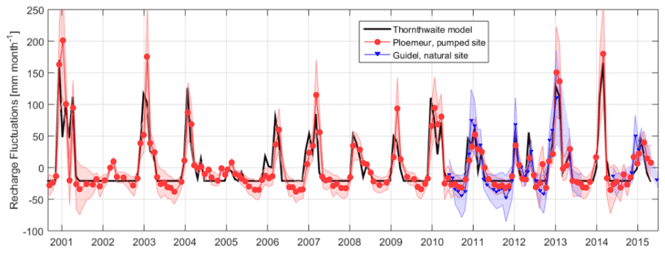
Figure 8 Monthly recharge fluctuations estimated from the groundwater analytical model at different boreholes at the Ploemeur (in red) and Guidel (blue) sites, propagating model parameter uncertainties. Shaded areas represent GW model uncertainty and variability between the different observation wells. Black line represents potential recharge fluctuations (anomalies compared to the mean value) from the Thornthwaite model.

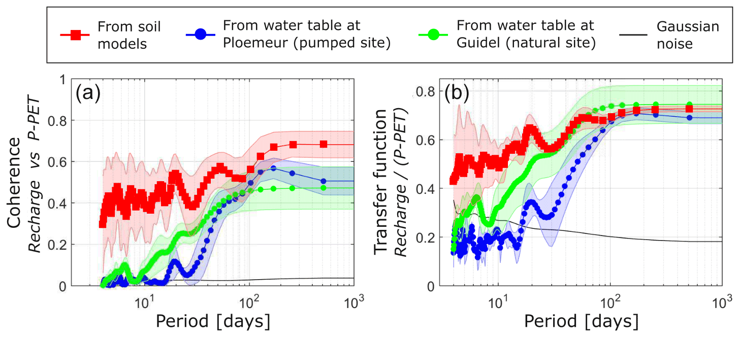
Figure 9 Coherence (a) and transfer function (b) between P−PET and recharge fluctuations estimated from the observed water table at Ploemeur (in blue) and Guidel (in green) sites or between P−PET and potential recharge fluctuations obtained from soil models. The coherence and transfer function of a 25 mm per month Gaussian noise is given as a reference (in black). Shaded areas illustrate the three soil model's range (Thornthwaite, GR4J, SURFEX) (in red) and the variability of estimated recharge fluctuations from several wells (in blue and green). P and PET refer to precipitation and potential evapotranspiration respectively.

On average, the Thornthwaite model overestimates analytically estimated RFs by 10 % to 20 %, though, for a few events, analytically estimated RFs can be larger. Based on these results, we can assert that recharge events greater than 25 mm per month can be detected with this method, as highlighted by single events that occurred in winter 2002 and 2005. Overall, RFs estimated from above and RFs performed with the GW analysis agree well at seasonal to long-term timescales. The main differences appear at the monthly scale or at shorter timescales. Therefore, here we compared RFs at a weekly timescale (not shown). At the Ploemeur site (respectively Guidel), the Thornthwaite model overestimates RF temporal variability obtained analytically from well F7 (respectively well PSR1) by 40 % (respectively 20 %), while both GR4J and SURFEX models fall within 5 %–6 %. In terms of the succession of recharge events, the correlation is 0.55, 0.58 and 0.65 for Thornthwaite, GR4J and SURFEX respectively, at the Ploemeur site. In general, Thornthwaite potential recharge events are ∼15 d ahead as compared to inverted RFs on Ploemeur site and slightly ahead with respect to the Guidel site. SURFEX performs better than other potential recharge models, better predicts all effective recharge events during dry years (2002, 2005) and wet summers (2004, 2012) but fails in describing intense recharge events.

5.3 The unsaturated zone and recharge fluxes

In Fig. 9, the coherence and transfer functions (Eqs. 7 and 8) between P−PET fluctuations and RFs inform on the efficiency of the transformation of rainfall events into recharge. These functions therefore illustrate the unsaturated zone response to rainfall in frequency domain. From Fig. 9, results can be summarized as follows: recharge estimated from soil models and recharge estimated from WTFs have similar long-term behavior, recharge estimated from soil models is too sensitive to rainfall in the short term and recharge estimated from WTFs is more sensitive to short-term events at the natural site compared to the pumped site.

Inverted RFs at both study sites (in blue and green in Fig. 9) and potential RFs (in red) are highly coherent with P−PET fluctuations (i.e., significantly larger than the expected coherence of Gaussian noise) over a wide range of frequencies, especially for periods larger than 100 d. As illustrated by the transfer function in Fig. 9, the amount of P−PET that recharges GW varies from <20 % at small temporal scales to >75 % at long-term timescales (typically seasonal timescale with winter rainy season).

Soil models generally fail to describe P−PET efficiency to recharge GW (i.e., the transfer function) at smaller timescales. Indeed, after episodic events, modeled potential recharge from three soil models (in red in Fig. 9) occurs more rapidly and with larger amplitudes as compared to RFs inferred from observed WTFs (in blue and green in Fig. 9). At the Ploemeur site, P−PET efficiency to recharge GW seems to be negligible (i.e., below the noise level) at periods below ∼30 d and climbs to maximum values for periods >100 d (in blue in Fig. 9b). Interestingly, coherence and transfer function between P−PET and recharge in Guidel (in green in Fig. 9) rise much earlier than in Ploemeur, beginning ∼10 d periods. This underlines a tighter link between P−PET and GW recharge in Guidel and a higher sensitivity to rainfall events.

Figure 9 shows that rainfall event distribution throughout the year impacts RFs because the transfer function between P−PET fluctuations and RFs inferred from WTFs is basically frequency-dependent. Intense rainfall events can generate GW recharge pulses. Mathematically, a single rainfall event is equivalent to a Dirac impulsion, of which the Fourier transform has a constant amplitude on all frequencies. The resulting recharge of such single rainfall events is therefore distributed on the whole spectrum, meaning that each rainfall event which is not consumed by evapotranspiration will necessarily be translated into recharge. Finally, recharge can occur during both (1) long/sustained winter rainfall and (2) episodic/intense rainfall events. We can also expect that recharge resulting from intense rainfall events will be more pronounced at the Guidel site because P−PET efficiency to recharge GW increases earlier at small temporal scales.

Overall, RFs estimated from GW levels can be described as a fraction of potential RFs using a linear regression when integrated at annual time step, but significant deviations exist in terms of amplitude and variability. The Thornthwaite RF equals 92 % of wet-season P−PET, while the RF from observed GW levels would suggest a range between 68 %–74 % at the pumping site and 77 %–110 % at the natural site where the GW level is close to the surface. At Ploemeur, the amount of seasonal recharge is therefore much lower than expected with the Thornthwaite model, while it can be larger at Guidel.

6 Discussion and consequences

6.1 The parsimonious strategy constrains hydrogeological characteristics well

6.1.1 Aquifer characteristic time constrained by aquifer characteristics: T, S and L

Here, we originally inferred GW properties based on WTFs measured in boreholes. These fluctuations generally bear typical frequencies from climatic and anthropic boundary conditions (hourly rainfall event, small diurnal variations due to evapotranspiration fall during the night, seasonal human water consumption, climatic cycles, etc.). They are also linked to the characteristic time of the system, and consequently to spatial scale. A first outcome of this work is that a simple physically based GW model can explain WTFs at the scale of the piezometric network, although local geological heterogeneities can play an important role, as shown in the steady-state case in Appendix C or by daily to monthly pumping tests (Le Borgne et al., 2006). A second outcome is that inferred equivalent hydraulic and geometric parameters are similar among boreholes and close to those obtained by previous modeling studies investigating the overall behavior of Ploemeur site. This provides confidence that the general aquifer behavior is well captured and that inferred parameters have some physical meaning. In addition, we stated that uncertainty on potential RFs, typically formulated by large-scale or conceptual soil models, was not critical to estimate GW parameters from long-term observed WTFs.

Aquifer characteristic time (L² S T⁻¹) controls how the distribution of recharge events is transferred laterally. Here, estimated characteristic time is typically 1.5 years. However, model length L here is a proxy of the distance between two streams. Considering that the model can be decomposed into two hillslopes of length $L/\mathrm{2}$, feeding rivers in x=0 and x=L, would reduce characteristic time to around 5 months. Such times appear short regarding the crystalline aquifer context. They appear much shorter than GW response time estimated from the worldwide parameter map in Cuthbert et al. (2019a) and than the “time to reach equilibrium” estimated for the biggest worldwide aquifers in Rousseau-Gueutin et al. (2013). However, aquifer length, constraining characteristic time, is much smaller here. Such estimates are in line with aquifer characteristic times typically inferred from streamflow and water quality data in the region (Guillaumot et al., 2021).

Here, storage coefficient values ($\mathrm{2}\times {\mathrm{10}}^{-\mathrm{2}}-\mathrm{1.5}\times {\mathrm{10}}^{-\mathrm{1}}$) are similar to those obtained in previous studies: S ranged from $\mathrm{5}\times {\mathrm{10}}^{-\mathrm{3}}$ to $\mathrm{5}\times {\mathrm{10}}^{-\mathrm{2}}$ for a recharge of 260 mm yr⁻¹ (Jimenez-Martinez et al., 2013) or from $\mathrm{2}\times {\mathrm{10}}^{-\mathrm{2}}$ to $\mathrm{6}\times {\mathrm{10}}^{-\mathrm{2}}$ for a recharge of 200 mm yr⁻¹ (Leray et al., 2012). Such values are much larger than expected for a crystalline context and larger than typical estimates from short-term pumping tests, where S ranged from 10⁻⁵ to 10⁻² (Le Borgne et al., 2006). We found that storage coefficient estimates typically depend on the length of the study period (Supplement), so that WTFs should be used for periods longer than 1 year typically for the Ploemeur and Guidel sites. This result, mostly based on seasonal timescales, suggests that the confined fractured aquifer is well connected to a more porous aquifer functioning as a storage compartment. Further discussion on this point can be found in Jimenez-Martinez et al. (2013).

In this work, transmissivity is estimated in the range $T\in [\mathrm{8}\times {\mathrm{10}}^{-\mathrm{4}}$; $\mathrm{8}\times {\mathrm{10}}^{-\mathrm{2}}]$ m² s⁻¹ (Fig. 6). Such large ranges are also found in Jimenez-Martinez et al. (2013) and Le Borgne et al. (2006), where $T\in [\mathrm{4}\times {\mathrm{10}}^{-\mathrm{3}}$; $\mathrm{4}\times {\mathrm{10}}^{-\mathrm{2}}]$ m² s⁻¹. Leray et al. (2012) calibrated a 3D model and defined a constant transmissivity T=2–$\mathrm{3}\times {\mathrm{10}}^{-\mathrm{3}}$ m² s⁻¹. Note that “local” transmissivity can be better estimated from pumping tests – which typically last several hours to several months – while storativity is highly affected by heterogeneity during such experiments (Le Borgne et al., 2006; Meier et al., 1998). This highlights the tight link between estimated hydraulic parameters and predominant boundary conditions at the timescale of the study (Cuthbert et al., 2019a).

6.1.2 On the representativity of GW levels

The steady-state approach shows the difficulty of obtaining relevant aquifer-scale information from mean GW levels because of local heterogeneities, incomplete sampling of the GW system and high sensitivity to model assumptions (Appendix C). Thus, heterogeneity largely impacts the ability to estimate mean GW recharge rate from GW levels. We found that WTFs observed in boreholes contain the overall aquifer response for observation periods around and larger than the aquifer characteristic time. RFs generate lateral GW flow that links different GW-level observations. For this reason, a single well contains information on aquifer-scale recharge, as underlined in the WTF approach. However, the WTF method alone has some limitations. We show that the well position within the GW flow system is as important as storativity to define recharge (geometric term in Eq. 5). Indeed, as recharge is transferred laterally, downstream wells will integrate the impact of both local and upstream recharge. Such behavior is expected to be even more pronounced if the well is located in a convergence zone (2D behavior). To go further, evapotranspiration losses in the downstream area could be inferred from boreholes located in the upstream area. This is probably already the case at Guidel; thus RFs would correspond to net RFs.

6.1.3 Limitations

The main assumptions of the GW model are (1) the 1D lateral flow structure, (2) homogeneous GW parameters and (3) uniformly distributed recharge. Regarding the 1D assumption on Ploemeur, pumping controls aquifer behavior so that the 1D assumption is valid over the system except close to the pumping wells. Pumping has generated a GW flow structure more or less constantly for 25 years. The water table does not interact with the surface. In this case, aquifer characteristic time is perfectly constrained and not borehole-dependent. At Guidel, GW intercepts the ground locally. Therefore, the flow structure is mainly driven by topography and is more complex, as highlighted by the different WTF patterns (Fig. 3). In this case, the system can be considered a set of 1D hillslope models. However, at Guidel, GW flow direction should be modified between seasons at boreholes close to rivers and wetland, making the 1D assumption less reliable. More generally, nonlinear GW–surface interaction (more pronounced during extreme dry or humid events) prevents WTFs being reproduced in such boreholes using 1D models. Indeed, model performance is limited for a few wells located close to rivers (PZ21, PSR15 and PZ17) but agrees well for other boreholes in the western part, where the aquifer characteristic time seems to converge.

We assumed that the heterogeneous system could be described by equivalent hydrodynamic properties. Previous works have highlighted that the behavior of complex aquifers could be described by equivalent homogeneous models when focusing on specific spatial and temporal scales (Clauser, 1992; Rovey and Cherkauer, 1995; Jimenez-Martinez et al., 2013; Herzog et al., 2021) or for well-connected fracture networks at large scale (Liu et al., 2016). While aquifer heterogeneity cannot be accurately captured and then represented in GW models, our results suggest that adding complex geological structures or considering a 2D geometry is not necessary to describe observed WTFs well in most boreholes . One limitation of this approach could be the effect of larger-scale heterogeneity in the geology such as transitions between lithological units. Indeed, in the case where a complex structure would affect the equivalent aquifer properties as a function of time, the analytical models will not be able to include such behavior.

The assumption of uniform recharge might be seen as unrealistic considering that local topographic and geological structures can favor exchanges between surface and groundwater (Favreau et al., 2009; Appels et al., 2015). It should be noted that the recharge period typically lasts 4 to 5 months, while GW behaves as an integrative system that smoothes out high-frequency recharge variability. In these conditions, it is expected that the deviation of recharge distribution does not alter the estimation of system-scale RFs.

Finally, note that the forward and backward models can be run at any – and different – time steps. The heart of the model is in the frequency domain, so that the first step consists in computing a Fourier transform to define amplitudes over a series of cosine functions. The number of frequencies is limited by the WTF sampling (Nyquist frequency). The recomposition in the temporal domain requires the cosine functions to be summed again, but all frequencies do not need to be used, and the temporal sampling can be adapted. Thus, applying the method requires time series of water levels at appropriate time steps to meet study objectives. To reduce computing time, parameter calibration can be done at bigger time steps; thus the potential recharge time series can be provided at this bigger time step. Here, we did it at a weekly time step, while RFs were computed from daily WTFs. We highlight that potential recharge can be a rough estimate or a first guess of RFs.

6.2 Relation between precipitation and actual GW recharge

The dependence of GW recharge to rainfall intensity and distribution throughout the year has been documented in several studies (Barron et al., 2012; Kendy et al., 2004; de Vries and Simmers, 2002; Gee and Hillel, 1988; Taylor et al., 2012). The same behavior is well demonstrated in this study, where annual RF amplitude cannot be fully expressed as a fraction of annual rainfall (see also Collenteur et al., 2021). For example, total P−PET during humid period is around 400 mm for different years, though RFs inferred from GW levels can differ by more than 100 mm.

Based on RFs estimated from WTFs, we highlight that the frequency-dependent relationship between P−PET and recharge can be described as a combination between a high-pass and a low-pass filter, which could represent the respective contribution of macropores and vertical unsaturated flow to recharge. It describes how both long-period seasonal rainfall and intense events participate significantly to recharge. Additional development should be carried out to link the shape of the transfer function (efficiency at high and low frequencies, cutoff frequencies) to the structure and hydrodynamic parameters of the unsaturated zone. In this work, we found that potential recharge estimated from soil models and recharge inferred from GW levels are fairly equivalent at seasonal to long-term timescales on the both sites, but they differ from short- to mid-term (< season) scale (Fig. 9). The tested soil models lack realism at short temporal scales (typically below 3 months), where recharge is often overestimated. Soil models are found to be too reactive to rainfall events, and they lack storage capacity.

The proposed approach allowed for computation of both RFs and associated uncertainties at seasonal timescales to reinvestigate the relationship between wet season P−PET and recharge. In addition, annual RFs estimated from GW levels can be described as a fraction of potential RFs using a linear regression. Thereby, the linear coefficient can be seen as a potential recharge partitioning coefficient. This partitioning coefficient should differ between Ploemeur and Guidel, assuming their potential recharge is similar. At Ploemeur, 74 % to 80 % of the potential recharge could be converted into groundwater recharge. For Guidel, this value ranges from 84 % to 100 %. The remaining part would be attributed to lateral flow within the unsaturated zone between the soil and the water table.

6.3 Pumping impacts recharge dynamics and main hydrogeological processes

6.3.1 Impact of the unsaturated zone thickness

The comparison between the Ploemeur and Guidel sites offers the opportunity to gain insights into the role of the unsaturated zone. Pumping thickens the unsaturated zone, so that potential recharge under the soil is first buffered in the deep unsaturated zone before generating GW recharge. We can infer that the unsaturated zone plays an inertial role by storing water and filtering out high-frequency variability. This is confirmed when looking at frequency-dependent time lags between P−PET and recharge (not shown), which is systematically larger at the Ploemeur site than at Guidel. Unsaturated zone thickness not only impacts the amount of recharge, but also the efficiency of rainfall to recharge GW at short-term (Fig. 9). We can conclude that setting up pumping can decrease recharge by negatively impacting the overall contribution of episodic recharge events. These results are in line with Cao et al. (2016) on the North China Plain.

6.3.2 Pumping stresses the deeper critical zone compartment

Inferred aquifer parameters slightly differ between the two neighboring sites, although they are located in the same geological context. On average, storage coefficients are larger and transmissivities smaller at the natural site (Guidel) than at the pumping site (Ploemeur). One interpretation of this result is that the weathered zone contributes more to GW flow at the Guidel site. Indeed, the weathered zone (0–20 m depth), known to be more porous and less permeable, should impact GW flow more when GW levels are closer to the surface. Conversely, at the Ploemeur site, the “deep” fractured aquifer controls flow as GW levels are all ∼15 m below ground. While aquifer characteristic times are similar at both sites, diffusivities ($T/S$) are typically larger at Ploemeur, meaning that aquifer length is longer. As a consequence, GW flow extends beyond the topographic limits of the catchment, as can be expected by the pumping (Fig. 1b).

7 Conclusions

The GW models developed here have several advantages. They manage to reproduce GW-level fluctuations (or anomalies) in heterogeneous aquifers well with three physical parameters and a limited execution time. We showed that GW-level fluctuations observed in one borehole contain aquifer-scale information at timescales equivalent to or larger than the aquifer characteristic time, while time-averaged groundwater levels are sensitive to heterogeneity. Therefore, the impact of local heterogeneities is smoothed out so that the aquifer-scale equivalent characteristic time and storage coefficient are reachable with limited dependence on prescribed potential recharge. The developed GW models are also invertible analytically to recover groundwater recharge fluctuations from observed GW-level fluctuation time series. A key novelty of this approach is developing the WTF method in the frequency domain. Note the method can be used to infer mean annual recharge value; however, we argue this is less relevant in heterogeneous aquifers.

The approach was tested at two neighboring sites, one that has been pumped for 25 years. First, recharge estimated from GW levels is coherent among each borehole, at each site. Second, the response to rainfall is more important when the unsaturated zone thickness is small for timescales <100 d. We finally showed how groundwater pumping mitigates high-frequency recharge events by thickening the unsaturated zone.

A large uncertainty in hydrological modeling lies in the fact that GW recharge can be derived from oversimplified conceptual soil models. Such an approach as described here gives hope that the GW heterogeneity issue could be overcome in hydrological models by defining the equivalent basin response with a similar frequency-domain analytical model. A similar approach has been designed to model streamflow variations in a bigger basin (Schuite et al., 2019). Several analytical solutions are provided at https://hplus.ore.fr/en/guillaumot-et-al-2022-hess-data (last access: 28 February 2022) considering either streamflow or GW-level fluctuations and considering different imposed boundary conditions.

In this study, the method is applied in crystalline contexts that display fractured aquifers, that are highly heterogeneous, which is challenging. Thus, similar approaches could be deployed in different geological contexts where GW-level time series are available over long timescales. In particular, it could be very interesting to test it in karstic aquifers. This method constitutes a useful alternative to study GW flows and recharge processes and their sensitivity to imposed boundary conditions, namely, precipitation and water use.

Appendix A: Development of the analytical groundwater model

A1 The 1D groundwater flow equation resolved in the frequency domain

The 1D diffusivity equation (also called GW flow equation), under the Dupuit assumption, and considering a non-leaky confined aquifer of uniform thickness or that the variations in the phreatic level are negligible compared to the aquifer thickness, can be written as (De Marsily, 1986)

$$\begin{array}{}\text{(A1)}& T{\displaystyle \frac{{\partial }^{\mathrm{2}}h(x,t)}{\partial x^{\mathrm{2}}}}=S{\displaystyle \frac{\partial h(x,t)}{\partial t}}-R\left(t\right),\end{array}$$

where h(x,t) denotes hydraulic head variations [L], R(t) the time-dependent, uniformly distributed recharge rate from the surface [L T⁻¹], T the aquifer transmissivity [L² T⁻¹] and S the storage coefficient of the aquifer [–]. Note that x is a Cartesian coordinate. This equation corresponds to a linearization of the Boussinesq equation. Time-dependent variables are then decomposed into the Fourier domain:

$$\begin{array}{}\text{(A2)}& f(x,t)=f_{\mathrm{mean}}\left(x\right)+\sum \mathrm{Re}\left\{\stackrel{\mathrm{‾}}{f}(x,\mathit{\omega })e^{i\mathit{\omega }t}\right\},\end{array}$$

where f_mean(x) is the steady-state term, and $\stackrel{\mathrm{‾}}{f}$ denotes complex Fourier coefficients depending on x and frequency ω. Re is the real part. Note that the first term of Eq. (A2) corresponds to ω=0 and will be solved separately. Note also that the number of frequencies, ω, is limited by the data sampling (Nyquist frequency). Inserting Eq. (A2) in Eq. (A1) (Carslaw and Jaeger, 1959) leads to the following second-order differential equation in x for each frequency, which does not depend on time after multiplication by e^−iωt:

$$\begin{array}{}\text{(A3)}& \begin{array}{rlr}& {\displaystyle \frac{{\partial }^{\mathrm{2}}\stackrel{\mathrm{‾}}{h}(x,\mathit{\omega })}{\partial x^{\mathrm{2}}}}-& {\displaystyle \frac{i\mathit{\omega }}{D}}\stackrel{\mathrm{‾}}{h}(x,\mathit{\omega })=-{\displaystyle \frac{\stackrel{\mathrm{‾}}{R}\left(\mathit{\omega }\right)}{T}}\\ & \mathrm{with}D={\displaystyle \frac{T}{S}},\end{array}\end{array}$$

where D is the hydraulic diffusivity [L² T⁻¹]. The transformation of the initial partial differential equation (from time t to pulsation ω) leads to a simpler second-order equation which admits a general solution of this form, for each Fourier mode:

$$\begin{array}{}\text{(A4)}& \stackrel{\mathrm{‾}}{h}(x,\mathit{\omega })=A\left(\mathit{\omega }\right)e^{x/X}+B\left(\mathit{\omega }\right)e^{-x/X}+\stackrel{\mathrm{‾}}{R}\left(\mathit{\omega }\right){\displaystyle \frac{X^{\mathrm{2}}}{T}}\end{array}$$

where $X=\sqrt{\frac{D}{i\mathit{\omega }}}$, and A, B and $\stackrel{\mathrm{‾}}{R}$ are all functions of ω.

In addition, the steady-state part of Eq. (A1) admits a range of solution of the form

$$\begin{array}{}\text{(A5)}& h_{\mathrm{mean}}\left(x\right)=C_{\mathrm{1}}{x}^{\mathrm{2}}+C_{\mathrm{2}}x+C_{\mathrm{3}}.\end{array}$$

Finally, by superposition, the general solution of Eq. (A1) is written

$$\begin{array}{}\text{(A6)}& \begin{array}{rl}h(x,t)=& C_{\mathrm{1}}{x}^{\mathrm{2}}+C_{\mathrm{2}}x+C_{\mathrm{3}}+\sum \mathrm{Re}\\ & \left\{e^{i\mathit{\omega }t}\left[A\left(\mathit{\omega }\right)e^{x/X}+B\left(\mathit{\omega }\right)e^{-x/X}+\stackrel{\mathrm{‾}}{R}\left(\mathit{\omega }\right){\displaystyle \frac{X^{\mathrm{2}}}{T}}\right]\right\},\end{array}\end{array}$$

where C₁, C₂ and C₃ refer to unknowns that can be determined from at least two boundary conditions.

A2 Defining boundary conditions

In Eq. (A1), GW recharge is taken into account as a time-variable term, uniformly distributed along the x axis of the model. Boundary conditions are applied on the two boundaries of the domain of length L (Fig. A1). Boundary conditions can be constant in time and/or time-variable. Boundary conditions can be of two kinds: (1) Dirichlet boundary conditions, where the value of h is specified, or (2) Neumann boundary conditions, where the derivative of h (i.e., flux) is specified.

Figure A1 Scheme of the analytical 1D groundwater model. Hydraulic head is variable along the x axis. Transmissivity T and storativity S are constant. Note that we consider an aquifer of uniform thickness with confined behavior under the Dupuit assumption so that the aquifer thickness does not matter in the model. (a) With boundary conditions corresponding to the pumping case. (b) With boundary conditions corresponding to the natural case (the solution is independent of the model width W).

The first model configuration described in Fig. A1a, corresponding to the Ploemeur pumping case, is defined by the following boundary conditions:

• at x=0, $Q(\mathrm{0},t)=Q_{\mathrm{pumping}}\left(t\right)=-TW\frac{\partial h(\mathrm{0},t)}{\partial x}$ (from Darcy's law)

• at x=L, $h(L,t)=h_L$.

The first boundary condition can be decomposed into one steady-state term Q_mean and a sum of coefficients $\stackrel{\mathrm{‾}}{Q}$ after a Fourier transform (Eq. A2). The second boundary condition appears as h_mean(L)=h_L in the steady part, which means $\stackrel{\mathrm{‾}}{h}(L,\mathit{\omega })=\mathrm{0}$ in the time-variable component. Thus, in the frequency domain and excluding the steady-state part (ω=0), the two boundary conditions can be written

• at x=0, $\stackrel{\mathrm{‾}}{Q}\left(\mathit{\omega }\right)=-TW\frac{\partial \stackrel{\mathrm{‾}}{h}(\mathrm{0},\mathit{\omega })}{\partial x}$

• at x=L, $\stackrel{\mathrm{‾}}{h}(L,\mathit{\omega })=\mathrm{0}$.

Inserting $\stackrel{\mathrm{‾}}{h}(x,\mathit{\omega })$ (Eq. A4) in these two boundary conditions leads to the next equations, where A(ω) and B(ω) as unknowns:

$$\begin{array}{}\text{(A7)}& \begin{array}{rl}& \stackrel{\mathrm{‾}}{Q}\left(\mathit{\omega }\right)=-{\displaystyle \frac{TW}{X}}\left[A\left(\mathit{\omega }\right)-B\left(\mathit{\omega }\right)\right]\\ & \mathrm{0}=\left(\mathit{\omega }\right)e^{L/X}+B\left(\mathit{\omega }\right)e^{-L/X}+\stackrel{\mathrm{‾}}{R}\left(\mathit{\omega }\right){\displaystyle \frac{X^{\mathrm{2}}}{T}}.\end{array}\end{array}$$

Thus, the analytical solution for the transient part is obtained once A(ω) and B(ω) are defined by solving the system of Eq. (A8) for the transient part. Then, each frequency is summed and passed to the time domain.

$$\begin{array}{}\text{(A8)}& \begin{array}{rl}h(x,t)& ={\displaystyle \frac{R_{\mathrm{mean}}}{\mathrm{2}T}}\left(L^{\mathrm{2}}-x^{\mathrm{2}}\right)+{\displaystyle \frac{Q_{\mathrm{mean}}}{WT}}(L-x)+h_L\\ & +\sum \mathrm{Re}\left\{e^{i\mathit{\omega }t}\left[\stackrel{\mathrm{‾}}{R}\left(\mathit{\omega }\right){\displaystyle \frac{X^{\mathrm{2}}}{T}}\left(\mathrm{1}-{\displaystyle \frac{\cosh \frac{x}{X}}{\cosh \frac{L}{X}}}\right)\right.\right.\\ & \left.\left.+\stackrel{\mathrm{‾}}{Q}\left(\mathit{\omega }\right){\displaystyle \frac{X}{TW}}{\displaystyle \frac{\sinh \frac{x-L}{X}}{\cosh \frac{L}{X}}}\right]\right\}\end{array}\end{array}$$

The steady-state part (left part of Eq. A8) was obtained by inserting h_mean(x) (Eq. A5) into the two following boundary conditions:

• at x=0, $Q_{\mathrm{mean}}=-TW\frac{\partial h_{\mathrm{mean}}(x=\mathrm{0})}{\partial x}$

• at x=L, $h_{\mathrm{mean}}(x=L)=h_L$.

The second model configuration described in Fig. A1b, corresponding to the Guidel natural case, is defined by the following boundary conditions:

• at x=0, $h(\mathrm{0},t)=h_{\mathrm{0}}$

• at x=L, $h(L,t)=h_L$.

So, such conditions appears as h_mean(0)=h₀ and h_mean(L)=h_L in the steady part and as $\stackrel{\mathrm{‾}}{h}(\mathrm{0},\mathit{\omega })=\stackrel{\mathrm{‾}}{h}(L,\mathit{\omega })=\mathrm{0}$ in the transient part. Thus, in the frequency domain and excluding the steady-state part (ω=0), the two boundary conditions can be written

• at x=0, $\stackrel{\mathrm{‾}}{h}(\mathrm{0},\mathit{\omega })=\mathrm{0}$

• at x=L, $\stackrel{\mathrm{‾}}{h}(L,\mathit{\omega })=\mathrm{0}$.

As for the pumping case, inserting $\stackrel{\mathrm{‾}}{h}(x,\mathit{\omega })$ (Eq. A4) into these two boundary conditions leads to a system of two equations with two unknowns (A(ω) and B(ω)). Thus, the analytical solution for this model can be obtained; it appears that this solution does not depend on the model width W. In this case, the only temporal dynamics are caused by the recharge.

$$\begin{array}{}\text{(A9)}& \begin{array}{rl}h(x,t)=& {\displaystyle \frac{R_{\mathrm{mean}}}{\mathrm{2}T}}\left(Lx-x^{\mathrm{2}}\right)+{\displaystyle \frac{h_L-h_{\mathrm{0}}}{L}}x+h_{\mathrm{0}}+\sum \mathrm{Re}\\ & \left\{e^{i\mathit{\omega }t}\left[\stackrel{\mathrm{‾}}{R}\left(\mathit{\omega }\right){\displaystyle \frac{X^{\mathrm{2}}}{T}}\left(\mathrm{1}+{\displaystyle \frac{\sinh \frac{x-L}{X}-\sinh \frac{x}{X}}{\sinh \frac{L}{X}}}\right)\right]\right\}\end{array}\end{array}$$

The steady-state part (left part of Eq. A9) was obtained by inserting h_mean(x) (Eq. A5) into the two following boundary conditions:

• at x=0, $h_{\mathrm{mean}}(x=\mathrm{0})=h_{\mathrm{0}}$

• at x=L, $h_{\mathrm{mean}}(x=L)=h_L$.

A3 Analytical inversion: solution to determine the recharge rate R(t)

Analytical solutions presented previously constitute a computationally much faster method than numerical models to represent hydraulic heads. They also offer the possibility to analytically recompute recharge rate R(t) from hydraulic head variations h(x,t).

As developed before, we will separate the steady state and the transient state. From Eqs. (A8) and (A9), the transient term of the hydraulic head can be written

$$\begin{array}{}\text{(A10)}& {\displaystyle }\begin{array}{rl}{h}_{\mathrm{transient}}(x,t)& =\sum \mathrm{Re}\left\{e^{i\mathit{\omega }t}\left[\stackrel{\mathrm{‾}}{R}\left(\mathit{\omega }\right){\displaystyle \frac{X^{\mathrm{2}}}{T}}\left(\mathrm{1}-{\displaystyle \frac{\cosh \frac{x}{X}}{\cosh \frac{L}{X}}}\right)\right.\right.\\ & \left.\left.+\stackrel{\mathrm{‾}}{Q}\left(\mathit{\omega }\right){\displaystyle \frac{X}{TW}}{\displaystyle \frac{\sinh \frac{x-L}{X}}{\cosh \frac{L}{X}}}\right]\right\}\end{array}\text{(A11)}& {\displaystyle }\begin{array}{rl}{h}_{\mathrm{transient}}(x,t)=& \sum \mathrm{Re}\left\{e^{i\mathit{\omega }t}\left[\stackrel{\mathrm{‾}}{R}\left(\mathit{\omega }\right){\displaystyle \frac{X^{\mathrm{2}}}{T}}\right.\right.\\ & \left.\left.\left(\mathrm{1}+{\displaystyle \frac{\sinh \frac{x-L}{X}-\sinh \frac{x}{X}}{\sinh \frac{L}{X}}}\right)\right]\right\}\end{array}\end{array}$$

respectively for the pumping and natural case. For each frequency (ω) we deduce that

$$\begin{array}{}\text{(A12)}& {\displaystyle }& {\displaystyle }\stackrel{\mathrm{‾}}{h}\left(\mathit{\omega }\right)=\stackrel{\mathrm{‾}}{R}\left(\mathit{\omega }\right){\displaystyle \frac{X^{\mathrm{2}}}{T}}\left(\mathrm{1}-{\displaystyle \frac{\cosh \frac{x}{X}}{\cosh \frac{L}{X}}}\right)+\stackrel{\mathrm{‾}}{Q}\left(\mathit{\omega }\right){\displaystyle \frac{X}{TW}}{\displaystyle \frac{\sinh \frac{x-L}{X}}{\cosh \frac{L}{X}}}\text{(A13)}& {\displaystyle }& {\displaystyle }\stackrel{\mathrm{‾}}{h}\left(\mathit{\omega }\right)=\stackrel{\mathrm{‾}}{R}\left(\mathit{\omega }\right){\displaystyle \frac{X^{\mathrm{2}}}{T}}\left(\mathrm{1}+{\displaystyle \frac{\sinh \frac{x-L}{X}-\sinh \frac{x}{X}}{\sinh \frac{L}{X}}}\right)\end{array}$$

respectively for the pumping and natural case. This leads to the following solutions:

$$\begin{array}{}\text{(A14)}& {\displaystyle }\begin{array}{rl}\stackrel{\mathrm{‾}}{R}\left(\mathit{\omega }\right)& =\left(i\mathit{\omega }S\stackrel{\mathrm{‾}}{h}(x,\mathit{\omega })-{\displaystyle \frac{\stackrel{\mathrm{‾}}{Q}}{XW}}{\displaystyle \frac{\sinh \frac{x-L}{X}}{\cosh \frac{L}{X}}}\right)\\ & \times {\left(\mathrm{1}-{\displaystyle \frac{\cosh \frac{x}{X}}{\cosh \frac{L}{X}}}\right)}^{-\mathrm{1}}\end{array}\text{(A15)}& {\displaystyle }\stackrel{\mathrm{‾}}{R}\left(\mathit{\omega }\right)=i\mathit{\omega }S\stackrel{\mathrm{‾}}{h}(x,\mathit{\omega }){\left(\mathrm{1}+{\displaystyle \frac{\sinh \frac{x-L}{X}-\sinh \frac{x}{X}}{\sinh \frac{L}{X}}}\right)}^{-\mathrm{1}}\end{array}$$

respectively for the pumping and natural case. Then, time domain recharge fluctuations (RFs) are computed by the inverse Fourier transform of $\stackrel{\mathrm{‾}}{R}\left(\mathit{\omega }\right)$ (Eq. A2). As only the transient state is developed here, RFs are equal to recharge rate variations minus the mean recharge rate along the studied period.

Appendix B: Validation of the analytical model

Following Cuthbert (2010), we tested our method with a virtual case using a ModFlow numerical model. This model is composed of one row and 200 columns with a mesh size of 10 m to obtain a 1D geometry. We simulated a confined layer of transmissivity $T=\mathrm{1}\times {\mathrm{10}}^{-\mathrm{3}}$ m² s⁻¹ and of storage coefficient S=0.05. Heads are imposed at x=0 and x=2000 m. By construction, the 1D numerical model is equivalent to the 1D analytical model used for the Guidel site (natural case).

B1 Simulating water table fluctuations from recharge fluctuations

GW-level fluctuations from the analytical and numerical models are compared. The imposed recharge was computed from the Thornthwaite soil model. To mimic the steady state of the analytical model, the initial condition in the numerical model is defined by applying a mean recharge rate. As illustrated in Fig. B1, both analytical and numerical solutions fit well. One main difference appears during the first 2 years because the analytical model does not consider any initial state. Indeed, the numerical model underestimates GW levels at the beginning of the simulation because the steady-state GW levels were used as initial state, while the simulation starts in January, during the humid period.

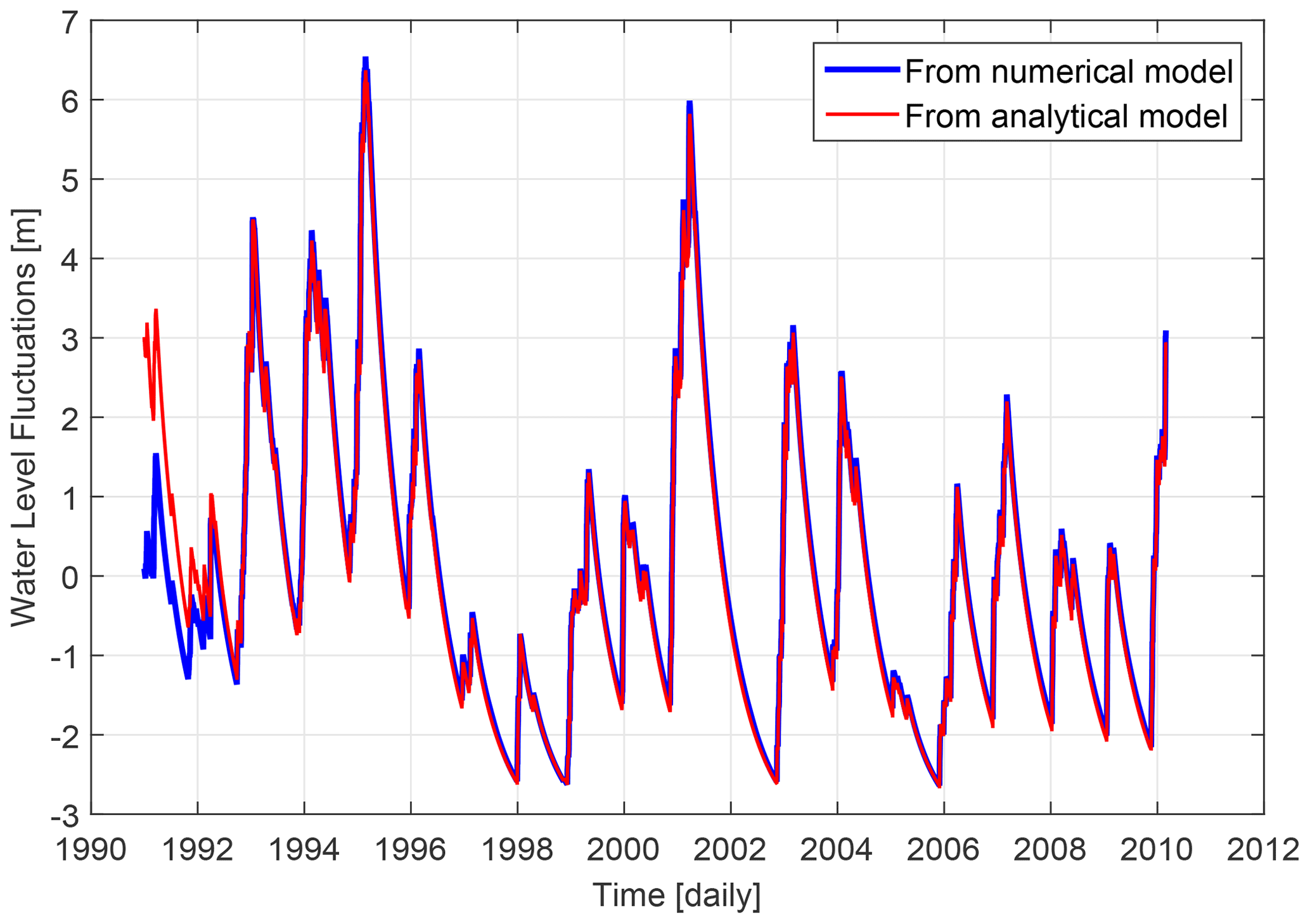
Figure B1 Comparison of water table fluctuations, at x=1500 m, obtained from analytical and numerical models. Note that the steady-state term (the mean value) has been removed.

B2 Accuracy of recharge inversion

In a second time, we performed a numerical test to estimate the ability of the analytic approach to estimate RFs. This experience is based on a comparison with the ModFlow model described previously. At the end of the numerical simulation, the hydraulic head at x=1500 m is recorded (blue curve in Fig. B1) and will be used to recover RFs analytically (Eq. A15). Then, these inverted RFs will be compared to the RFs imposed on the ModFlow model. We tried to answer two questions, namely (1) at which timescale recharge is well estimated and (2) what the impact of parameter uncertainties on RF estimates is.

Although the analytical model can be run at the same time step as the well data, RF estimates are affected by (1) numerical oscillations linked to the discrete frequency-domain computations over a finite length time series and (2) the amplification of high-frequency GW head variations, including observation errors. Estimated RFs can be integrated over time to avoid these spurious oscillations. Overall, an integration time larger than a few original time steps is sufficient to ensure an estimation of the recharged volume at a 99 % level (Fig. B2). An accurate recovery of temporal variations, though, requires integration over 10 time steps to reach determination and correlation coefficients r, r²>0.95.

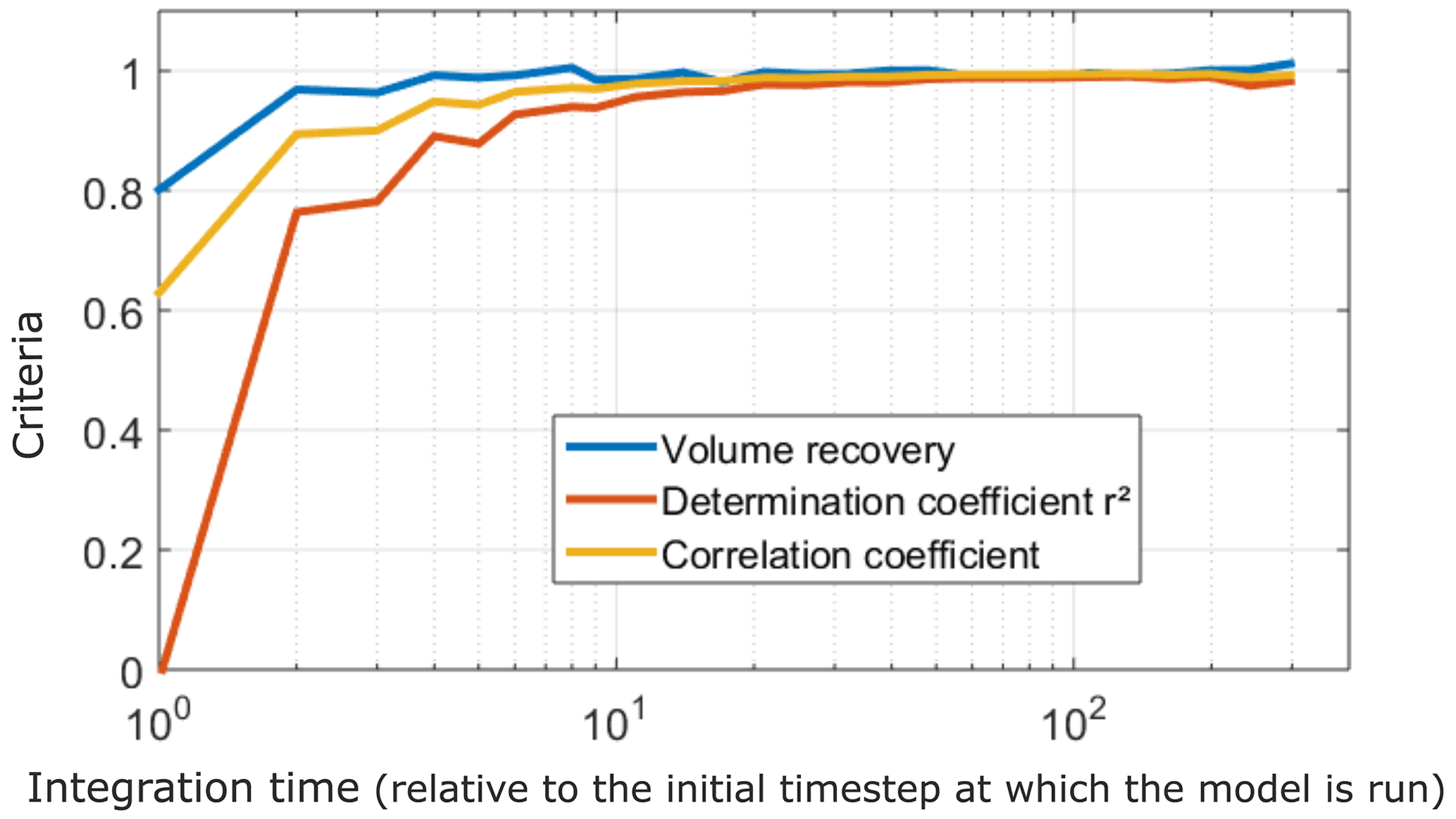
Figure B2 Impact of integration time on recharge volume, determination coefficient r² and correlation coefficient between inferred and true (initially imposed to the numerical ModFlow model) recharge. “Volume recovery” refers to the ratio between inferred and true mean annual amplitude.

Figure B3 Impact of uncertainties on the estimation of characteristic time t_c on recharge amplitude (defined by the “volume recovery”, equal to the ratio between inferred and true mean annual recharge amplitude) and timing recovery (defined by the correlation coefficient). The gray rectangle defines the typical uncertainty on estimated characteristic time.

This test also gives an idea of parameter uncertainties. We can see how RFs estimated from GW levels are influenced in terms of timing and mean amplitude. Parameter (T, S and L) uncertainty logically has an important impact. However, uncertainty on characteristic time has a limited impact on both timing and amplitude of RFs, as shown in Fig. B3.

Appendix C: Mean groundwater level and mean recharge estimates

We explored the stationary part of Eq. (A8) (pumping case), defining the relationships between aquifer transmissivity, long-term mean recharge and flow. In theory, and in homogeneous media, $R_{\mathrm{mean}}/T$ can be directly estimated from the quadratic shape of the water table (Eq. A8), i.e., the deviation of mean GW level with respect to a linear evolution. In Fig. C1, mean GW levels observed at Ploemeur are projected along the x axis and are compared to one of the best steady-state model. Note that in Fig. C1, modeled mean GW level has a quadratic component, while it appears mostly linear. In spite of this apparent good restitution of mean GW levels, equifinality on parameters (R_mean, T, L and h_L) occurs. It is clear that heterogeneity affects mean GW levels deeply, so that separating the impact of recharge and heterogeneity on mean GW level is difficult.

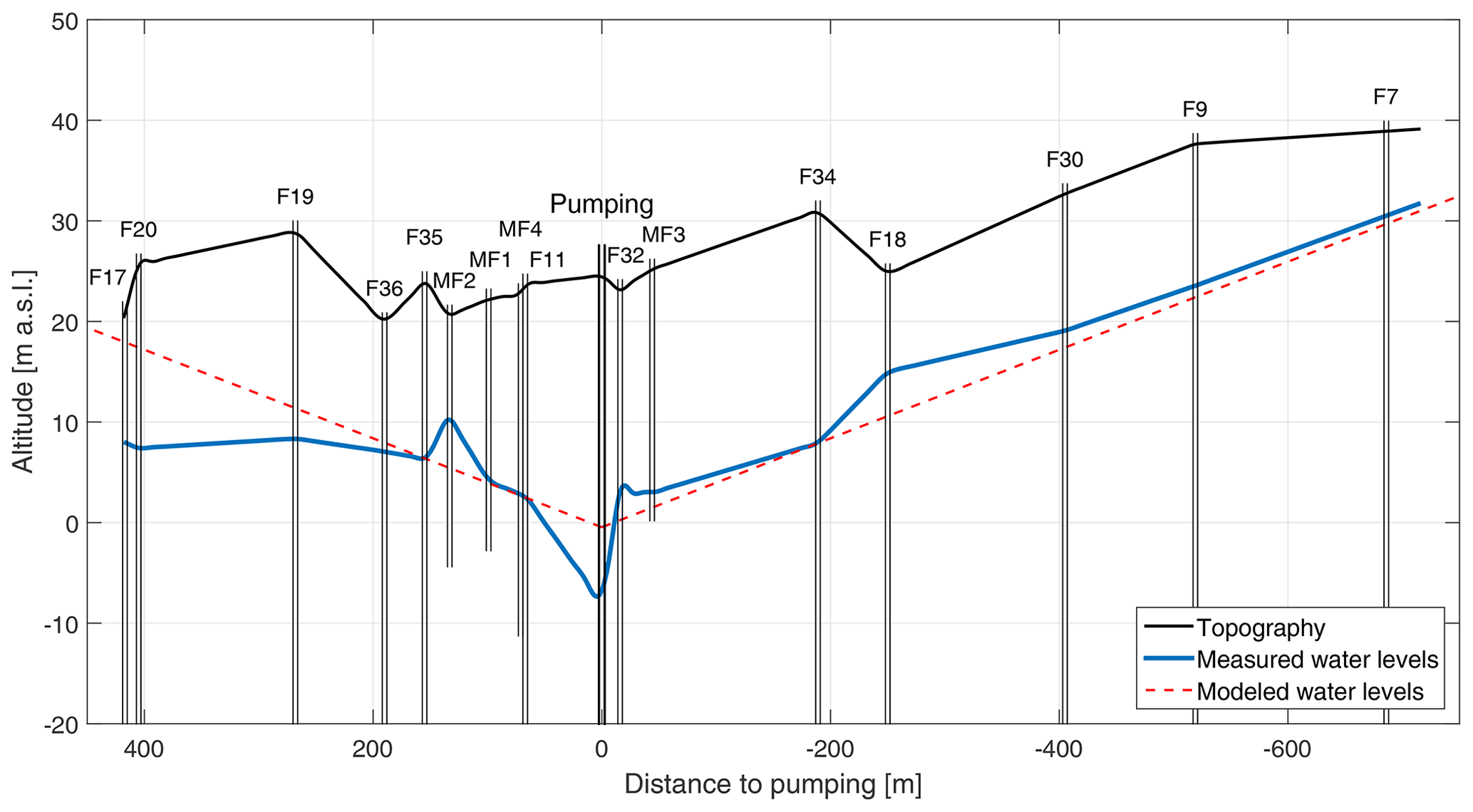
Figure C1 Mean groundwater levels observed at the Ploemeur pumping site (blue curve), shown on a SE–NW cross section. The dashed red curve represents the best 1D steady-state analytical model, which has the lowest least-square difference between data and the model.

In addition, we investigated this steady-state issue using a numerical homogeneous 2D MODFLOW model. The actual 10 m resolution topography was imposed as upper-boundary conditions (DRAIN PACKAGE), and pumping wells were set up at their actual position in the domain with their respective pumping rates. The advantage of such a model was to set a realistic geometry and to remove geometric parameters like model length L and imposed head h_L (steady-state term of Eq. A8). So, we only kept two parameters in this calibration: mean recharge rate (R_mean) and transmissivity (T). Results showed that T and $R_{\mathrm{mean}}/T$ ratio seems well constrained when focusing on mean water levels measured in several boreholes. However, T and $R_{\mathrm{mean}}/T$ estimates are not relevant because they are sensitive to the boreholes selected for the calibration and to the presence of potential heterogeneities.

Finally, the information content of mean GW levels is limited by (1) incomplete sampling within the observation network, considering the punctual nature of borehole data with respect to local heterogeneities in recharge and hydrodynamic properties, blurring the evolution of hydraulic head in space (Fig. C1); (2) incomplete sampling of the GW system as the observation network represents only a limited part of the aquifer; and (3) limitations linked to hypotheses in the conceptual model. Uncertainties in actual boundary conditions, such as the representation of local GW behavior close to the pumping wells, also limit interpretation. The inability to constrain transmissivity and mean recharge from long-term mean well observations is in line with several studies (e.g. Sánchez-Vila et al., 1996).