the Creative Commons Attribution 4.0 License.
the Creative Commons Attribution 4.0 License.
 | 27 Oct 2022
FarmCan: a physical, statistical, and machine learning model to forecast crop water deficit for farms
Sara Sadri
James S. Famiglietti
Hylke E. Beck
Aaron Berg
Eric F. Wood
In the coming decades, a changing climate, the loss of high-quality land, the slowing in the annual yield of cereals, and increasing fertilizer use indicate that better agricultural water management strategies are needed. In this study, we designed FarmCan, a novel, robust remote sensing and machine learning (ML) framework to forecast farms' needed daily crop water quantity or needed irrigation (NI). We used a diverse set of simulated and observed near-real-time (NRT) remote sensing data coupled with a random forest (RF) algorithm and inputs about farm-specific situations to predict the amount and timing of evapotranspiration (ET), potential ET (PET), soil moisture (SM), and root zone soil moisture (RZSM). Our case study of four farms in the Canadian Prairies Ecozone (CPE) shows that 8 d composite precipitation (P) has the highest correlation with changes (Δ) of RZSM and SM. In contrast, 8 d PET and 8 d ET do not offer a strong correlation with 8 d P. Using R2, root mean square error (RMSE), and Kling–Gupta efficiency (KGE) indicators, our algorithm could reasonably calculate daily NI up to 14 d in advance. From 2015 to 2020, the R2 values between predicted and observed 8 d ET and 8 d PET were the highest (80 % and 54 %, respectively). The 8 d NI also had an average R2 of 68%. The KGE of the 8 d ET and 8 d PET in four study farms showed an average of 0.71 and 0.50, respectively, with an average KGE of 0.62. FarmCan can be used in any region of the world to help stakeholders make decisions during prolonged periods of drought or waterlogged conditions, schedule cropping and fertilization, and address local government policy concerns.
- Article
(5734 KB) - Full-text XML
- BibTeX
- EndNote


The Food and Agricultural Organization (FAO) estimates that global food production must increase 50 %–70 % by 2050 to feed the projected population of 10 billion (UN/ISDR, 2007; FAO, 2009). Combined with the increasing frequency of drought due to climate change, non-sustainable use of groundwater, and increasing competition from municipal, environmental, and industrial water needs, farmers are facing the challenge of maximizing crop production without a growing water supply (Han et al., 2018). Farmers across the world, however, may lack adequate means to characterize crop water use, and thus agricultural water management often operates under conditions of unknown water deficiency (Levidowa et al., 2014). Therefore, identifying crop water stress in different growing seasons is necessary to predict yield conditions and plan irrigation scheduling (Virnodkar et al., 2020). Needed irrigation (NI) or irrigation consumptive water use (ICU) is the amount of water to reduce crop water stress, satisfy crop water demand, and enhance agricultural water use efficiency (WUE; Kirda, 2000). In irrigated farms, information on NI can help regulate water deficit, achieve higher levels of crop produced per unit of water consumed, and optimize profit while minimizing potential negative environmental effects (Han et al., 2018; Chalmers et al., 1981; Taghvaeian et al., 2020). However, information on the proper quantity of water to feed crops is also essential in rainfed areas with insufficient rainfall to maintain crop yields and soil conditions (Virnodkar et al., 2020). As climate change and recurring drought continue to impact crop water stress levels and food security, rainfed farms in the U.S. and Canada are increasingly adopting irrigation technologies (USDA-NASS, 2021). For example, the Canadian Ministry of Agriculture is encouraging farmers in Saskatchewan to evaluate their potential NI and apply for irrigation development (Saskatchewan Government, 2022). Knowing the quantity and timings of the water supply gives farmers incentives for more efficient practices such as adopting irrigation, identifying the timing and amount of fertilizer supply, and facilitating more extensive insurance planning and adaptation strategy goals (White et al., 2020; Levidowa et al., 2014; Stocker et al., 2013; Geerts and Raes, 2009; Taghvaeian et al., 2020). The timely determination of NI has shown to save water and energy and help farmers achieve improved yields and quality (USDA-NASS, 2021). Several main approaches have been investigated to determine the temporal variability in NI and crop water stress. These methods are based on soil water status, plant responses, and crop modeling using remote sensing data (Taghvaeian et al., 2020; Virnodkar et al., 2020). Most crop water deficit studies have focused on model-based crop water stress, mostly because of the difficulty of measuring water availability for specific agricultural periods such as crop growth or yield (Ash et al., 1992; Wittrock and Ripley, 1999; Quiring, 2004). There have been limited implications for monitoring and predicting farm-specific NI without using in situ data (Jia et al., 2011). Therefore, providing accurate short-term forecasts of irrigation depth and timing is challenging for soil water balance modeling and other scheduling strategies (Taghvaeian et al., 2020). Smilovic et al. (2016) and Andarzian et al. (2011) employed the crop water model, AquaCrop, to evaluate the timing and spatial distribution of irrigation water between farms within a watershed in western Canada. They showed that wheat production alone could be maintained while reducing water use by 77 %, and production could increase by 27 % without increasing irrigation water use. Despite their advantages, NI and crop water stress models can have limited spatial and temporal availability for input data, can be too complicated to operate, and cannot easily be operated as a forecasting tool using remote sensing data. Plant hydraulic models, for example, have relatively complete mechanistic representations of humidity, temperature, and leaf area index (LAI), but they are usually too complex, with many parameters that are hard to measure for crops (Yang et al., 2020).
With near-real-time (NRT) remote sensing, farm NI modeling with reasonable confidence and the potential for better-informed water resources management is now achievable, especially in areas where access or more advanced on-farm technologies are too costly. Remote sensing has been used to calculate vegetation indices (Romero et al., 2018), measure changes in photosynthetic pigment cells (Poblete et al., 2017), measure canopy content and water balance in leaves (Rapaport et al., 2015), and estimate the surface energy balance (Allen et al., 2007). Over the past few decades, machine learning (ML) techniques also have been progressively used to process large amounts of information created by remotely sensed data. Several studies have indicated the high significance of addressing plant water stress using ML, which will help farmers improve water and cropland management practices in the low water productivity areas, substantially enhancing the food security (Virnodkar et al., 2020). Various machine learning algorithms, such as random forests (RFs), support vector machines (SVMs), artificial neural networks (ANNs), genetic algorithms (GAs), and ensemble learning, have been used on remote sensing information in farming (Virnodkar et al., 2020). RF applications have become popular for addressing data overfitting, especially in geospatial classification and prediction of remote sensing data (Vergopolan et al., 2021; Saini and Ghosh, 2018). Poccas et al. (2017) used RF and SVM to model leaf water potential for assessing grapevine water stress. Loggenberg et al. (2018) combined RF with remote sensing data to distinguish stressed and non-stressed Shiraz vines. Despite these advances, scientific NI applications for evaluating crop water stress using remote sensing data have generally remained limited, with relatively low adoption by farmers (Virnodkar et al., 2020; Yang et al., 2020; ScienceDaily, 2021). Some of the problems to date are as follows:
-
Lack of access. Many farmers across the globe do not have access to the results of NI models. Therefore, management practices mostly rely on farmers' experience rather than scientific NI models.
-
Lack of timely predictions. Producers need to make NI decisions several days in advance and require tools capable of accurately forecasting short-term crop water use.
-
Complex procedures. Many of these models have tenuous requirements for inputs, time, labor, and financial investment, making the model remain within the scientific domain and out of reach for potential users.
To improve crop water stress and NI deficit management, focus should be on (1) including short-term forecasts in NI schedulers, (2) reducing data, time, labor, and cost requirements for schedulers, (3) providing user-friendly decision support systems, and (4) incorporating remotely sensed data in scheduling (Taghvaeian et al., 2020).
Table 1Land use from 2015 to 2019.
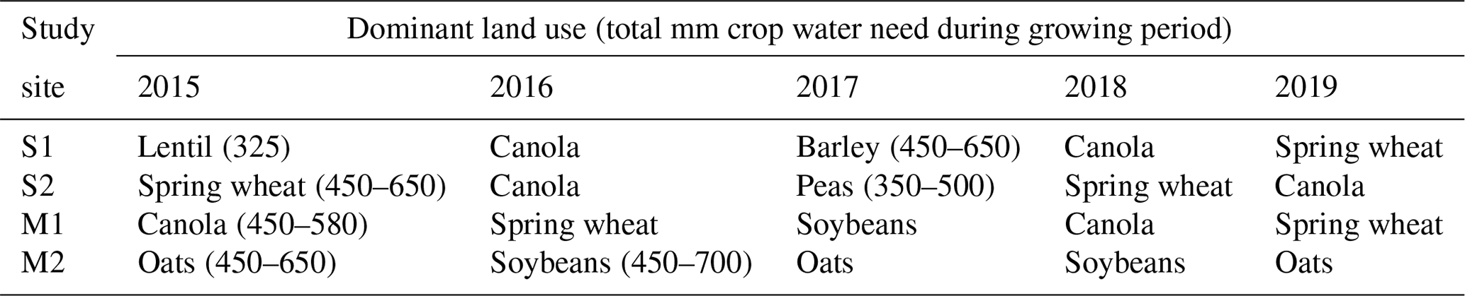
Average crop water use is from FAO guidelines.
In this study, we developed the FarmCan model to address the abovementioned issues. FarmCan is a hybrid physical–statistical–ML model for NI scheduling and other agricultural applications. At its core, FarmCan is trained on NRT remote sensing data such as surface soil moisture (SM), root zone soil moisture (RZSM), precipitation (P), evapotranspiration (ET), and potential ET (PET) to monitor and forecast daily NI daily and up to 14 d in advance. The contributions of the FarmCan algorithm are to (1) use farm-specific NRT remote sensing data as inputs, (2) use ML to forecast PET, SM, and RZSM using P prediction, (3) develop a climate-informed forecast of crop NI volume and timing with up to 14 d lead time, (4) allow users to interact with the tool by finding their farms, choosing crop and growing days, and joining a plan that guides and informs them about NI through the growing season, and (5) use SM or RZSM, depending on the timing and crop growth stage. Our framework is customized for the Canadian Prairies Ecozone (CPE). However, the methodology is generic and can be transferred anywhere to inform farmers and stakeholders where and when additional water is potentially needed to compensate for water deficits. The tool will provide valuable information to governments', agriculturalists', and industries' sustainable initiatives to grow more food and avoid waste with better-managed water; however, ultimately adaptation decisions will need to be made in a more extensive community and through government dialogue within management goals.
The remainder of this paper is organized as follows: Sect. 2 describes the study area and the datasets used to train FarmCan. Section 3 describes the FarmCan model structure and development. Section 4 presents the performance and validation of model results. Major conclusions of the study are presented in Sect. 5.
2.1 Study area
Over 80 % of Canadian farms are concentrated in the CPE – i.e., southern portions of Alberta (AB), Saskatchewan (SK), and Manitoba (MB; Wheaton et al., 2005). The CPE has some of the world's highest climate and weather variability. It is predominately continental with long, cold winters, short, hot summers, and relatively low precipitation amounts during the short growing season of May to September (Bonsal et al., 1999). The annual mean precipitation is around 478 mm, of which rainfall accounts for almost two-thirds of it during the growing season, and snowfall makes up another 30 % of it. Average winter and summer temperatures are −10 and 15 ∘C, respectively (Hadwen and Schaan, 2017). Such variabilities significantly affect the CPE's agriculture, environment, economy, and culture yearly (Sadri et al., 2020). For example, the drought of 2001–2002 cost approximately USD 3.6 billion in agricultural production losses (Wheaton et al., 2005). Between 2008 and 2012, federal–provincial disaster relief payouts for climate-related events totaled more than USD 785 million and more than USD 16.7 billion in crop insurance. The 100-year record-breaking drought in 2017 caused massive wildfires, reduced yields (particularly canola), heat stress, poor grain fill, livestock feed shortages, and the relocation of nearly 3000 cattle in Saskatchewan and Alberta (Cherneski, 2018). The vulnerability of the CPE to agricultural production risks and the future scenarios of climate, which show more severe and frequent droughts with declining precipitation trends and surface water resources during summer and fall, makes the region ideal for developing and testing robust crop NI methodologies.
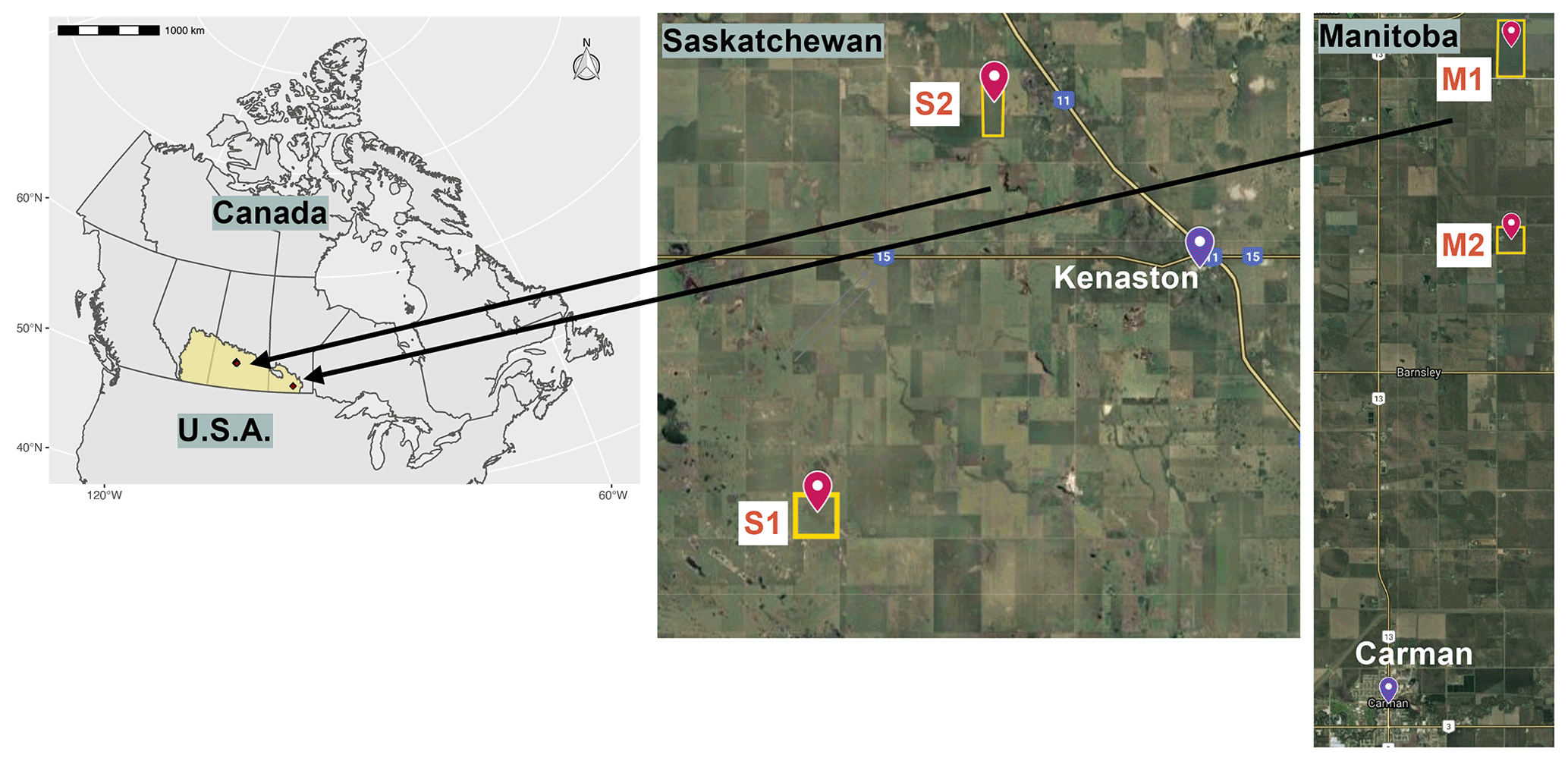
Figure 1Locations of the four study farms in Saskatchewan (S1 and S2), near Kenaston, and in Manitoba (M1 and M2), near Carman (© Google Earth 2021).
Table 2Information about each of the four study sites (data from 2015 to 2019).
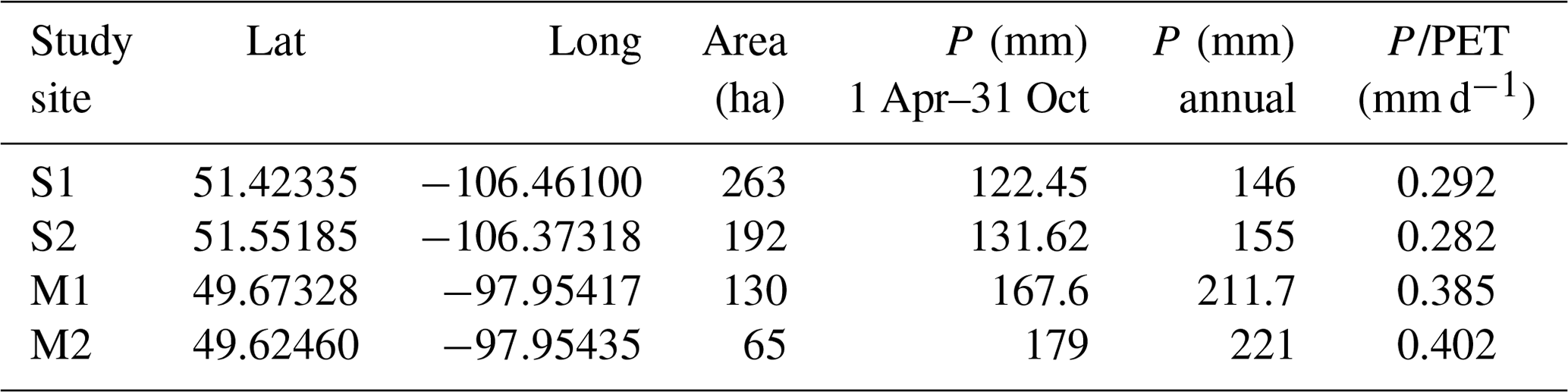
P/PET is the aridity index. PET is the potential ET obtained from National Atlas of Canada.
A total of four study farms, on average 160 ha each, were selected within the provinces of SK and MB (Fig. 1). These farms are sites for other soil moisture core validation networks, such as the Agriculture and Agri-Food Canada (AAFC) RISMA (Real-Time In-Situ Soil Monitoring for Agriculture) network (Bhuiyan et al., 2018) and the Kenaston Network in Saskatchewan for NASA Soil Moisture Active Passive (SMAP) validation (Sadri et al., 2020; Tetlock et al., 2019). All four farms are rainfed and have alternating crop years (ECCC, 2013). Farmers use pasture, spring wheat, shrubland, and other cover crops to avoid farrow and water-logged conditions in spring. Depending on field and weather conditions, planting typically occurs in late April and early May. For this study, we consider a fixed 7-month window for the growing season from 1 April to 31 October. Table 1 shows that, between 2015 to 2019, at least seven different crops were planted on the four study farms. Most crops were canola and spring wheat, although there were also soybeans, oats, barley, peas, and lentils. These crops have low to medium sensitivity to drought, and their root depth at maximum growth is anywhere from 0.6 m (lentils and soybeans) to 1.5 m (canola, barley, and spring wheat). The average crop water needs through the growing season are 550 mm; much less was provided by rain, as shown in Table 2 (Shuval and Dweik, 2007; Brouwer and Heibloem, 1986). Table 2 shows the amount of precipitation during and outside the growing season. Precipitation outside the growing season is primarily snow. Wind plays a critical role in moving and blowing snow. Therefore, the contribution of melting snow toward meeting future crop water requirements is not substantial and not considered in the FarmCan model. However, establishing soil water reservoirs or having stubble fields (Pomeroy et al., 1990) can improve snow contribution to SM in the future. Comparing PET with the total annual precipitation, we expect to confirm that the amount of water supplied by precipitation is insufficient to meet optimum crop growth.
Each farm's growing season aridity index (P/PET) is shown in the last column of Table 2. This index is used across the globe to represent vegetation's biogeographical distribution and estimate crop yield (Franz et al., 2020). Based on the aridity index, Manitoba farms have a higher expected crop yield than Saskatchewan farms.
2.2 Model components
The two main requirements for the datasets to develop FarmCan are the (1) availability of at least 5 years' worth of NRT remotely sensed data and (2) accessibility of such data in real time. These two factors would make the FarmCan algorithm trainable and updatable daily. Various datasets were considered, such as leaf area index (LAI) and the ET from the NASA ECOSTRESS satellite (ECOsystem Spaceborne Thermal Radiometer Experiment on Space Station; Fisher et al., 2017), but they did not meet one or both of the requirements. On the other hand, MODIS (Moderate Resolution Imaging Spectroradiometer) ET and PET products are available and accessible in NRT at 500 m pixel resolution. The Multi-Source Weighted-Ensemble Precipitation (MSWEP) can provide global P values with a 3 h 0.1∘ resolution covering the period 1979 to the near present (Beck et al., 2019) as an NRT or forecasted product. PET, ET, and P are critical predictors of crop water stress that link the water–energy–carbon cycle (Pendergrass et al., 2020; Brust et al., 2021). SMAP SM products (surface and root zone) are also available and accessible in NRT and provide a highly accurate descriptor of crop stress globally (White et al., 2020). SM is a direct measure of agricultural drought (Sadri et al., 2020; Vergopolan et al., 2021). RZSM becomes important during particular growth stages (mid season and late season) and affects crop growth at maturity stage and final crop yield (Smilovic et al., 2019). The inclusion of SM as a dynamic parameter within crop water stress numerical modeling has improved forecast capabilities (Tetlock et al., 2019; Wanders et al., 2014; Koster et al., 2009). The datasets used in this study are listed in Table 3.
Entekhabi et al. (2014)Reichle et al. (2019)Beck et al. (2019)Running et al. (2019b)Running et al. (2019b)Table 3Datasets and the periods used to train and run the model in this study. All input variables were clipped to the CPE domain.
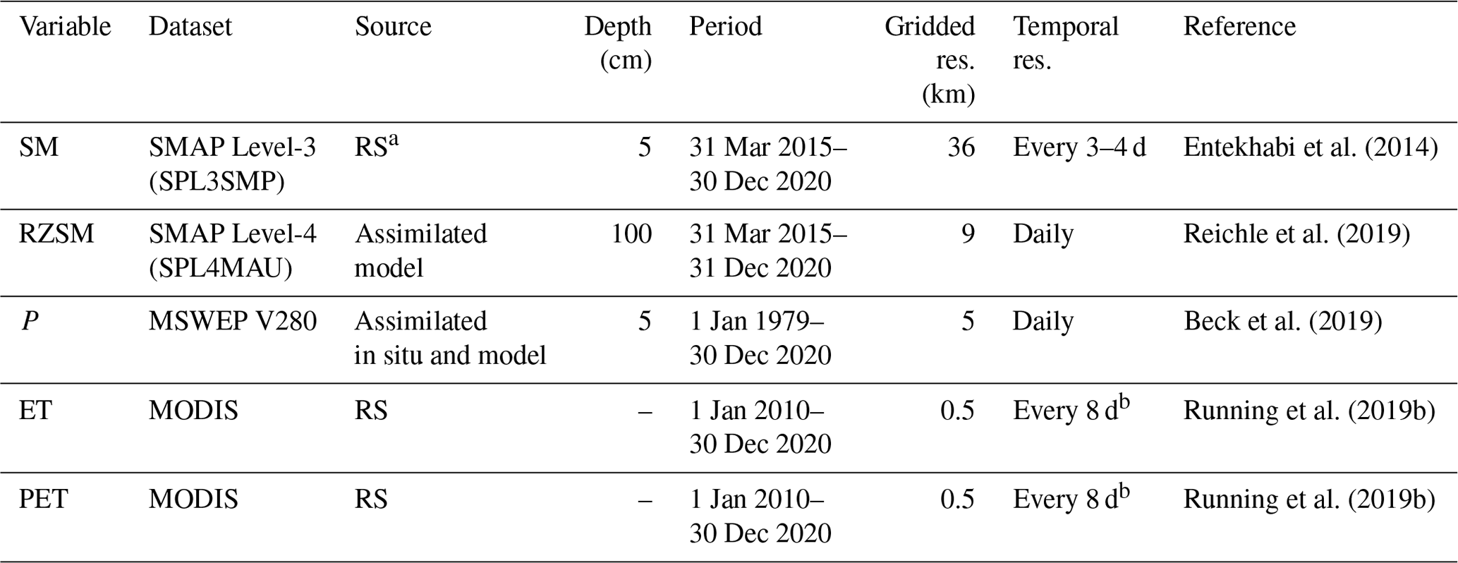
a RS is for remote sensing. b The 8 d composite values.
The SMAP satellite was launched in 2015, and the data are available from 31 March 2015 to the present. SMAP level 3 SM (0–5 cm; SPL3SMP) is a composite based on daily passive radiometer retrievals of global land SM in the top 5 cm of the soil that is resampled to a global, cylindrical ∼36 km Equal-Area Scalable Earth Grid, version 2.0 (EASE-Grid 2.0). For this study, we used version 4 of SPL3SMP retrievals from the morning overpasses to minimize uncertainties and bias from the in situ data (Al Bitar et al., 2017).
The SMAP level 4 (SPL4SMAU) is a daily global RZSM product (0–1 m) obtained by assimilating low-frequency (L-band) microwave brightness temperature observations (for which SPL3SMP is the gridded version) into the GEOS-5 catchment land surface model (CLSM; Reichle, 2017; Reichle et al., 2015; Sadri et al., 2018), which is driven by surface meteorological data from the NASA Goddard Earth Observation System (GEOS) weather analysis (Brust et al., 2021; Rienecker et al., 2008). Additional corrections using gauge- and satellite-based precipitation estimates downscale to the model's temporal and 9 km scale (Liu et al., 2011; Reichle et al., 2011).
ET and PET data are derived from MODIS, a modified MOD16A2/A3 Terra version 6 (Running et al., 2019a) ET/latent heat flux algorithm. The units are 0.1 kg m−2 per 8 d (i.e., 0.1 mm per 8 d), which is the summation of total daily ET through 8 d (Running et al., 2019b). The last acquisition period of each year is a 5 or 6 d composite period, depending on the year. The algorithm used for the MOD16 data product collection is based on the Penman–Monteith equation, which includes inputs of daily meteorological reanalysis data along with MODIS remotely sensed data products such as vegetation property dynamics, albedo, and land cover. Provided in the MOD16A2 v006 product are layers for composited ET and PET along with a quality control layer from 1 January 2001 to the present. MODIS data are available from 2010 to the present.
MSWEP version 1 (0.25∘ spatial resolution) was released in May 2016 and since then has been applied regionally and globally for modeling SM and ET (Beck et al., 2019; Martens et al., 2017), estimating plant rooting depth (Yang et al., 2016), evaluating root zone soil moisture patterns (Zohaib et al., 2017), evaluating climatic controls on vegetation (Papagiannopoulou et al., 2017), and analyzing diurnal variations in rainfall (Chen and Dirmeyer, 2017) and various other applications (Beck et al., 2019). The product blends gauge-, satellite-, and (re)analysis-based P estimates to improve the accuracy of the estimates globally. MSWEP is a global P product with a 3 h 0.1∘ resolution covering the period 1979 to the present. It does not provide a forecast. However, MSWEP V280 is largely consistent with a newer product, MSWX, that offers medium- and longer-term forecasts. Here, we used past dates to build a forecasting tool, so using the MSWEP V280 product was sufficient. For future software development applications, we will use MSWEP combined with MSWX to provide real-time forecasts (Beck et al., 2022).
We used the data in Table 3 in the parsimonious NI model of the FAO as follows:
where NI is the volume of water needed to compensate for the deficit between PET as a demand factor, P, and change in soil moisture content (ΔSM or ΔRZSM) as supply factors. All units in Eq. (1) are in millimeters. To take care of the unseen delays among system components and to reduce errors, we use 8 d composite periods in Eq. (1) and throughout this study. The use of 8 d is also consistent with the MODIS output data format.
To convert ΔSM or ΔRZSM volumetric values to depth in Eq. (1), we multiplied their values by the corresponding depth of the soil (mm; Pereira et al., 2015; Allen et al., 1998). For example, a 0.2 m3 m−3 of the surface SM (in the first 50 mm of the topsoil) is equivalent to mm d−1, whereas the same volumetric soil moisture for the root zone (with a consistent depth of 1000 mm) is equivalent to mm d−1, meaning that 200 mm of water can be drawn from 1 m deep soil. FarmCan uses 50 or 1000 mm depth, depending on the crop's development stage. When the crop is in stages 1 or 2, the algorithm uses the first 50 mm depth, and when the crop is in stages 3 or 4, 1000 mm depth is used.
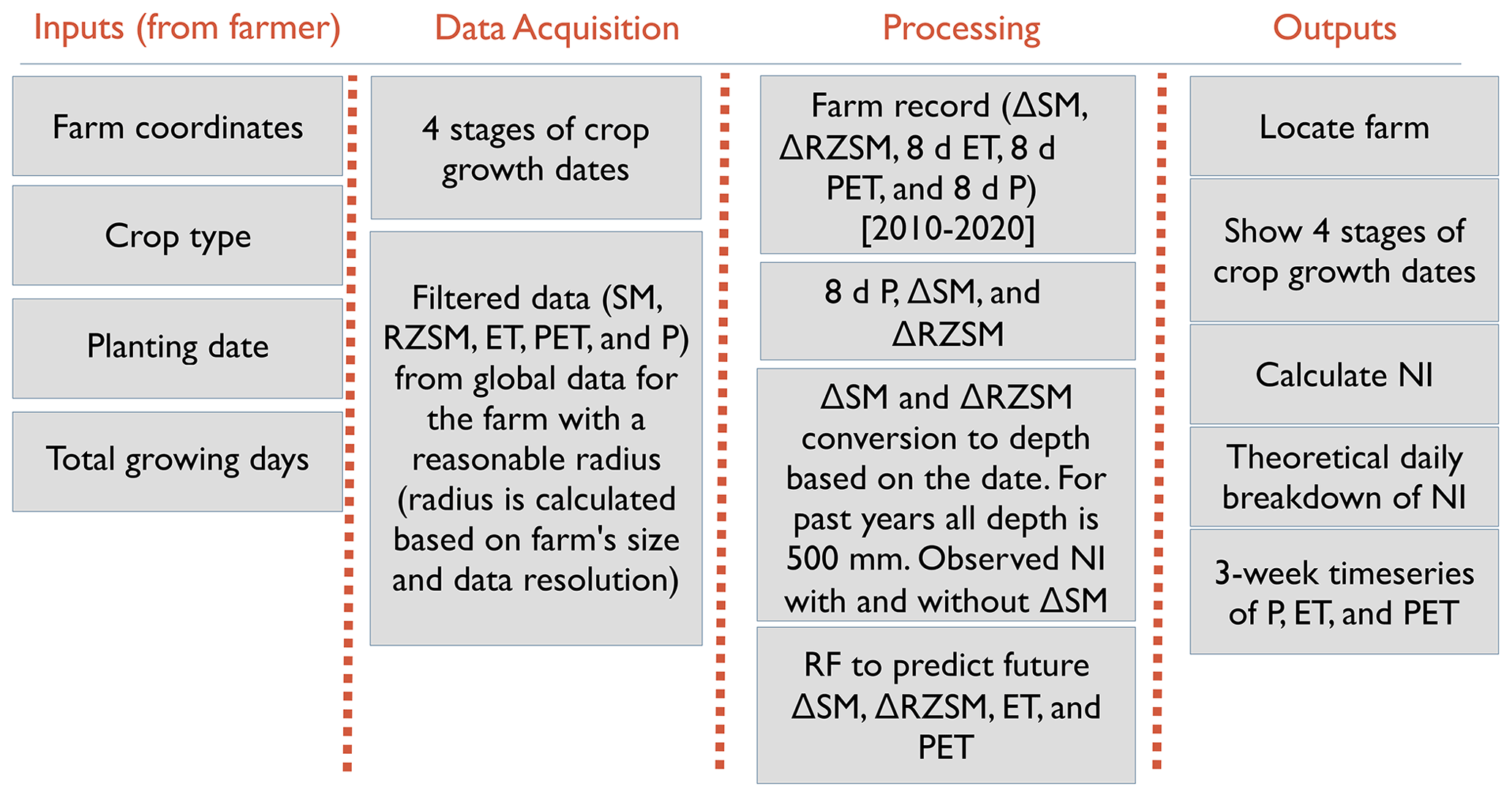
Figure 2 summarizes the design of the main steps for the FarmCan algorithm. The steps include the following:
-
The user inputs the coordinates of a farm, crop type, planting date, and total growing days.
-
The algorithm locates the farm and calculates the dates of each of the four phenological stages of crop growth.
-
From the farm coordinates, the farm center is calculated. Gridded data (i.e., P, SM, RZSM, ET, and PET) are clipped from the primary datasets using radii from the farm center calculated in such a way that each radius for each variable includes the closest gridded data surrounding the farm perimeter. Calculations of the variables' radii are based on trial and error and the variable's spatial resolution. The farm's specific variable time series is filtered by interpolating the grids outside the perimeter and any of the grids inside the farm. Time series data are further processed for the 8 d composite or changed (Δ) values.
-
The variable with the highest correlation with the 8 d P would be the first predictand used to train a random forest (RF) algorithm. RF then forecasts that variable for up to 2 weeks. The predicted variable would then be fed jointly with the 8 d P as predictors in the next step to predict the next highly correlated variable on the list. The process repeats in a feeding loop, and in every round, a new variable is first predicted and then used as a predictand.
-
Using Eq. (1), the 8 d NI (NItotal) is calculated. If there was no precipitation over the past 8 d, for every antecedent day i, NIi is NI, where i ∈ [1, 2, …, 8]. However, for any amount of P in an antecedent day i, NItotal should be adjusted, as less supplementary water is needed to compensate for moisture deficit for the days with Pi>0. We calculate daily adjusted weights as follows:
where is
For example, day i with no precipitation has % of the Ptotal, and a day with 45 % of Ptotal has a %. The value of 800 is the total deficit percentage in the absence of no rain. The daily distributed amount of NI over 8 d is then calculated as follows:
To check the correctness of the calculations above, the relationship should hold true.
3.1 Random forest (RF) algorithm
RF (Breiman, 2001) is an ML method that has shown high accuracy in the function estimation and nonparametric regression of geospatial hydroclimatic and spaceborne data (Clewley et al., 2017; Vergopolan et al., 2021). The RF algorithm aggregates the predictions made by multiple decision trees of varying subsets called the bagged or bootstrapped datasets. Showing trees different training sets is a way of de-correlating them (Sonth et al., 2020). It also decreases the variance in the model without increasing the bias, ultimately leading to better model performance. Furthermore, while the predictions of a single tree are highly sensitive to noise in its training set, the average of many trees is not, as long as the trees are not correlated. The FarmCan model uses RF in two stages, i.e. (1) to fill in the gaps of missing ΔSM and ΔRZSM, based on 8 d P from 2010 to 2020, and (2) to predict ΔRZSM, ΔSM, 8 d ET, and 8 d PET up to 14 d in advance. We divided the datasets from 2010 to 2020 into training and testing in a 0.7 to 0.3 ratio.
The first round of running RF uses 500 decision trees. The optimum number of trees is the one that minimizes the mean square error (MSE) between the training and testing datasets. The second round of running RF involves dictating the optimum number of trees. If a training set X=x1, … xn (n being the number of training samples) has responses Y=y1, … yn, then the algorithm selects random samples with the replacement of the training set for B times. In Eq. (5), for b=1, … B training samples from X and Y, called Xb and Yb, we produce a regression tree fb. After training, predictions for unseen samples x′ can be made by averaging the predictions from all the individual regression trees.
4.1 Spatial comparison of hydrological variables
Figure 3 shows the key variables' 20th, 50th, and 80th percentiles from 2015 to 2020 during the growing season (April to October). Comparing P with the ET and PET map shows that, region-wide, crops do not receive the water needed from rain to reach an optimal yield. The growing season's P is typical of sub-humid and semi-arid climates (Pereira et al., 2015), i.e., the amount of rainfall is often not sufficient to satisfy the water needs of crops. Except for portions of the province of AB, most CPE farming relies on rainfall and, therefore, is vulnerable to agricultural drought (Maybank et al., 1995; McGinn and Shepherd, 2003; White et al., 2020).
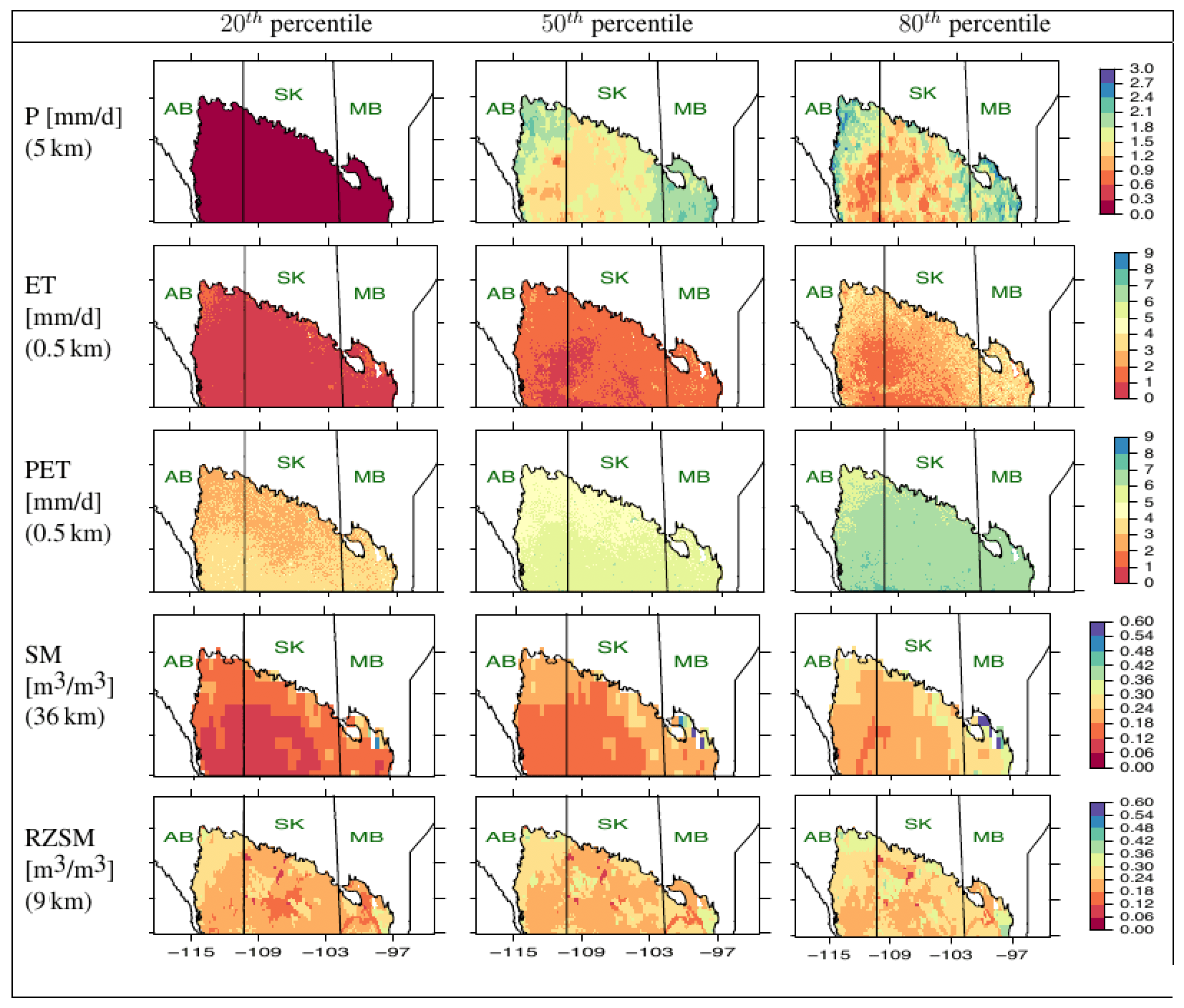
Figure 3Spatial patterns of variables used for the CPE. Data collected from 2015 to 2020 for the agricultural months (April–October). AB is Alberta, SK is Saskatchewan, and MB is Manitoba.
Most of Saskatchewan is identified by the lowest amount of SM, P, and ET throughout the growing season. Surface SM is generally lower than RZSM across all three provinces. This is expected as soil at the surface is affected directly by transpiration and wind. In contrast, the soil at the root zone holds onto the water longer, especially as brown-black Chernozemic clay, a typical type of soil in the CPE.
4.2 Relative importance of FarmCan inputs
We ran a two-by-two Pearson correlation analysis with a 99 % significance level for the four selected farms and during the 7-month growing seasons from 2015 to 2020 (Fig. 4).
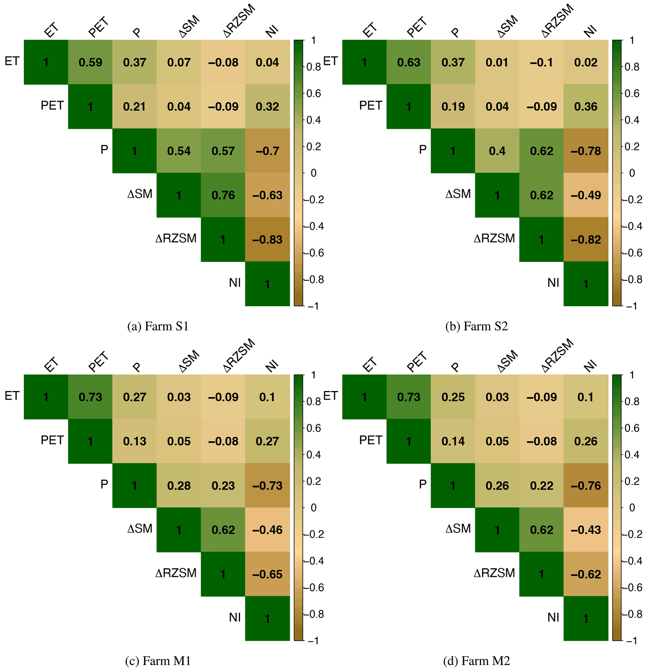
Figure 4Pearson correlation relationship between observed 8 d ET (mm per 8 d), PET (mm per 8 d), P (mm per 8 d), ΔSM (m3 m−3), ΔRZSM (m3 m−3), and NI (mm per 8 d) for farms S1, S2, M1, and M2 during agricultural years (2015–2020). Significance level of 99 %.
The four farms' results show that the correlation between P and ΔRZSM and P and ΔSM is quite similar in M1 and M2. However, the correlation between P and ΔRZSM is slightly higher in S1 and considerably higher in S2. Although it is generally expected that instantaneous surface soil moisture shows more variability with P, this study is based on the 8 d cumulative P and changes in 8 d SM and not a direct measure of P vs. SM. For example, if the total amount of P over 8 d is 20 mm, the RZSM can change from 0.2 to 0.9 m3 m−3, which gives a higher ΔRZSM than ΔSM, which might have fluctuated instantaneously but essentially changed from 0.3 to 0.5 over 8 d. However, more studies in different regions must confirm such correlations. We speculate that soil type plays a role in how soil maintains moisture at different depths.
There is also no evidence of significant feedback from ET to SM, and vice versa. This can be because the relationship between SM and ET, in terms of feedback, mainly depends on the climate (Seneviratne et al., 2010). During the growing season, the condition in CPE is either too wet, which makes the total energy for ET independent of SM, or too dry, which makes ET show little impact on fluxes because it is little or no moisture available.
Generally, a significant impact of SM on ET should be more noticeable in a transitional regime where soil water supply is available and sufficient (Yang et al., 2020; Running et al., 2019b; Seneviratne et al., 2010; Famiglietti and Wood, 1994). More studies from different regions are required to understand such interactions in SM and ET fluxes.
All four farms show a significant negative correlation between soil moisture values with 8 d NI within 99 % confidence.
4.3 Feedback from a supply–demand mechanism
To study the relationship between water supply and demand in the CPE, we conducted a three-way comparison of changes in 8 d P supply with variability in ΔSM and ΔRZSM (supply). We also included changes in 8 d ET and 8 d PET (demand factors) in a correlation plot shown in Fig. 5. Each row represents a province with the supply variables on the XY axes. For each region, the two left-hand plots show the relationship between 8 d P and ΔSM. Color changes correspond with 8 d PET and 8 d ET. The two right-hand plots are the same, except that the Y axis represents ΔRZSM instead of ΔSM.
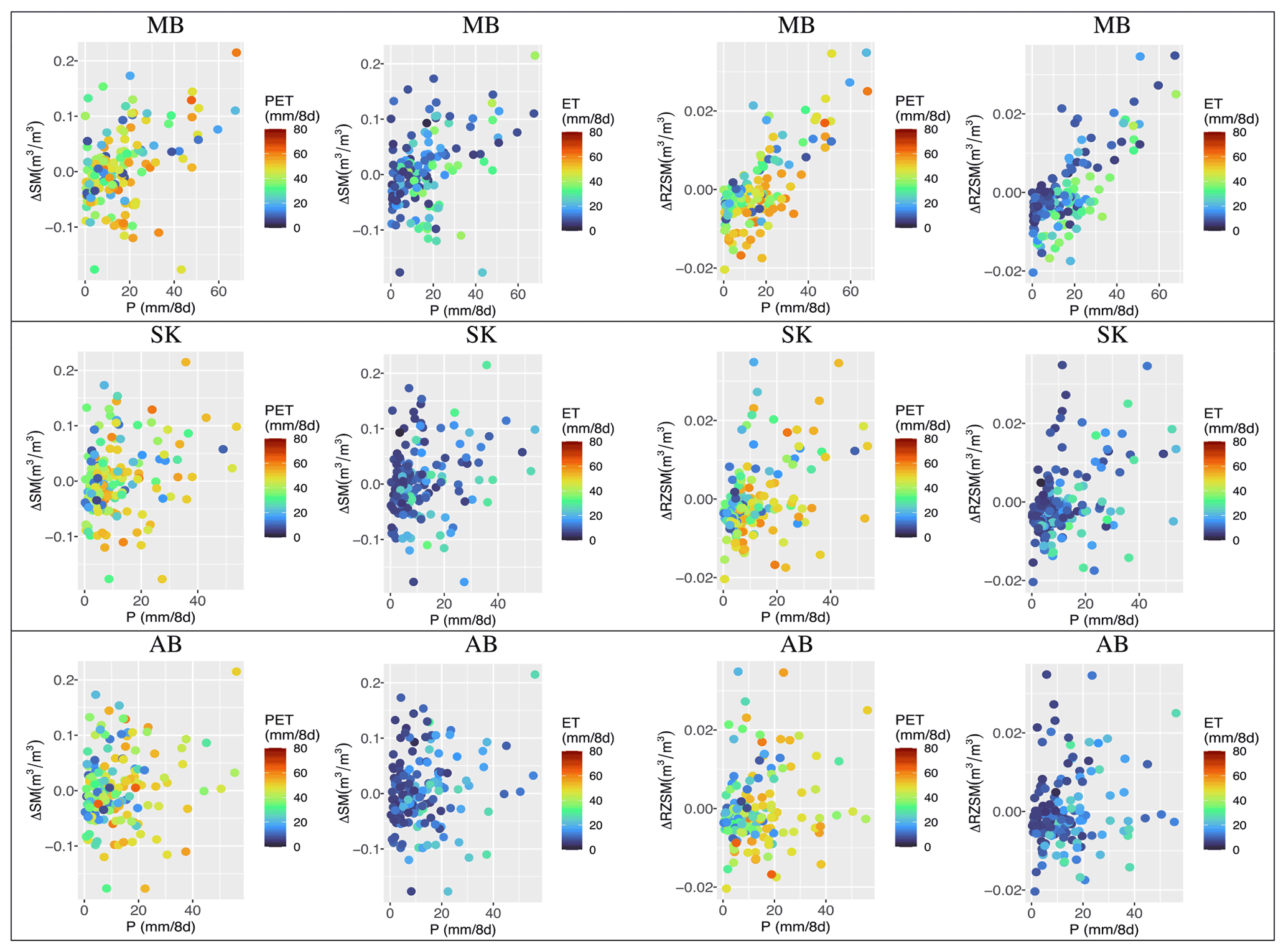
Figure 5Changes in 8 d P, ΔSM, and ΔRZSM (supply) with 8 d ET and 8 d PET (demand). Each row shows one province. Data were collected from 2015 to 2020 for the agricultural year (April–October).
Manitoba shows the most robust linear relationship between 8 d P and ΔRZSM. In contrast, Alberta shows the weakest linear relationship between 8 d P and ΔRZSM, likely because most Alberta farms are artificially irrigated. ΔRZSM is more responsive to the amount of 8 d precipitation, meaning that, over an 8 d increase in P, RZSM increases. Such a linear relationship is weaker between 8 d P and ΔSM. This can be because surface SM is also affected by exposure to other physiological elements such as wind, elevation, transpiration, and land cover.
There are also visible linear relationships between the 8 d PET and 8 d P, especially in Manitoba and Saskatchewan. The 8 d PET (and less for 8 d ET) tend to increase with higher 8 d P. The 8 d ET and 8 d PET do not show a linear correlation to the ΔSM, although for periods for which 10 mm < 8 d P < 40 mm, 8 d PET values tend to have a positive trend when the ΔSM is decreasing (negative). When 8 d P>40 mm, Saskatchewan and Alberta showed more mid-range PET (20–60 mm per 8 d). This can mean that SK and AB are regularly in dry conditions when the water supply is less than optimum. MB is generally moist but can range from adequate crop water availability to extreme water stress periods. The atmospheric demand is typically low for periods with 8 d P less than 10 mm. In all plots, the average 8 d PET is higher than the 8 d ET, which shows that a higher-than-supplied atmospheric demand exists throughout the growing season at the CPE.
4.4 Time series of data and calibration period
Figure 6 is the variability plot of Farm S2 from 2015 to 2020. Each year's 7-month agricultural period is shown with a pink background. A negative ΔSM or ΔRZSM means a decrease in SM or RZSM, respectively, over the 8 d intervals, and vice versa.

Figure 6An 8 d variability analysis for Farm S2 (2015–2020). The pink background indicates the agricultural period. Green is PET, red is ET, purple is ΔSM, black is ΔRZSM, and teal is 8 d P.
During every agricultural year, the SM reacts to P with much higher variability and sensitivity than ΔRZSM. Although instantaneous rain is more correlated with the SM, as previous results showed, 8 d P shows a higher correlation with Δ RZSM. In the CPE, ΔRZSM generally reverts to zero, indicating a weakly stationary behavior. However, the amount and timing of daily RZSM can still be insufficient to support effective crop growth. As for surface SM, the changes do not seem stationary. The 8 d PET is consistently higher than 8 d ET, confirming that crops receive less than the optimal amount of their water demand throughout the year. We plotted variability plots for the other three farms (not shown here), and the patterns were consistent with those from Farm S2.
4.5 FarmCan prediction process
To illustrate the FarmCan real-time forecast process, we describe an example in which 2 July 2020 is “today's date”, the crop type is barley, the planting date is 1 April 2020, and the whole growing season is 150 d. The FarmCan algorithm uses these inputs and the FAO guidelines to provide the expected dates of stages 1 to 4, as shown in Table 4.
Table 4Key dates relevant to barley planted on 1 April 2020 (from FAO guidelines; Pereira et al., 2015).
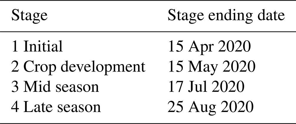
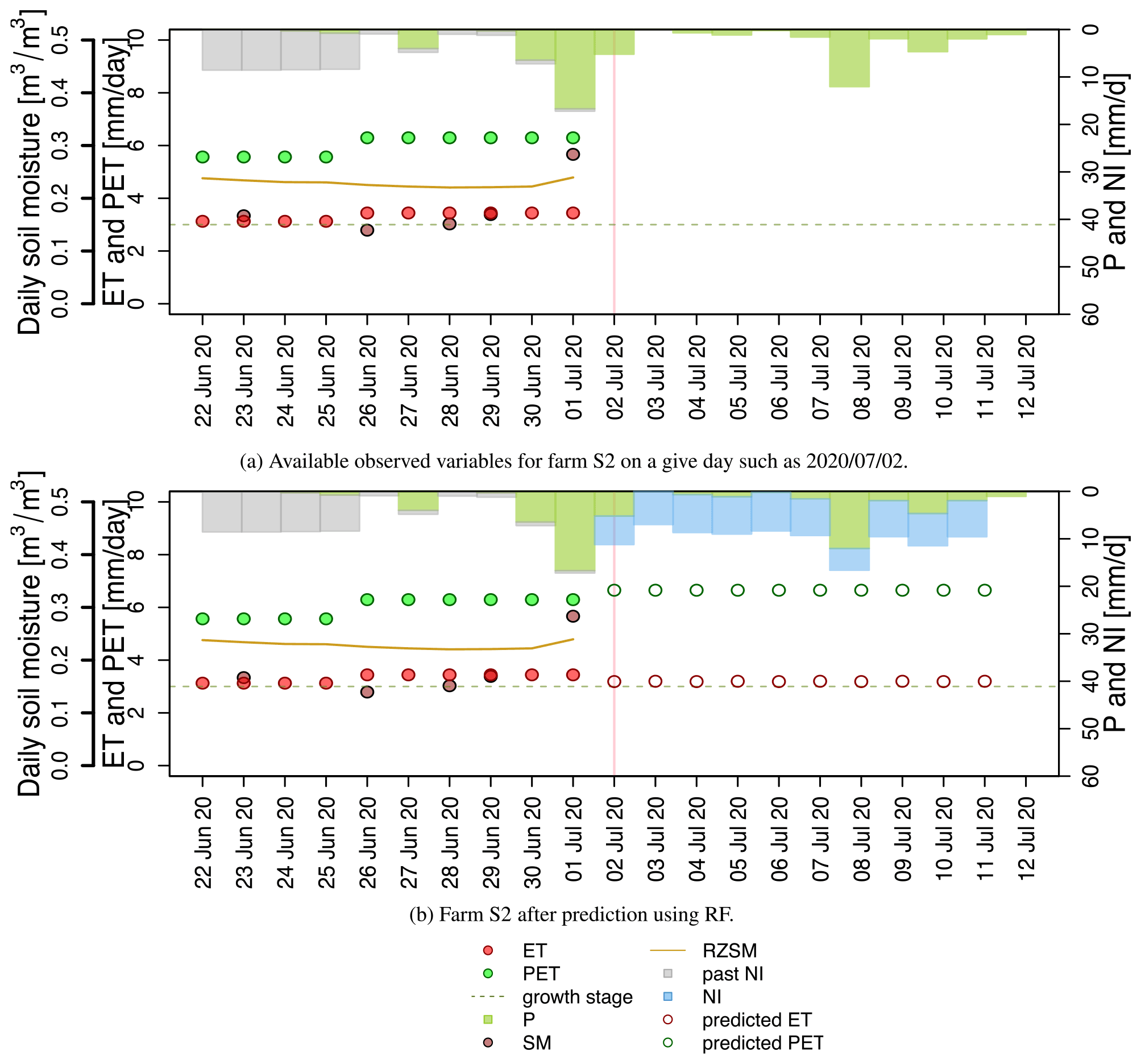
Figure 7Farm S2 before and after prediction relative to the date 2 July 2020. Over the next 10 d, the total predicted PET is 67 mm, total predicted ET is 32 mm, total P is 30 mm, and NI is 71 mm.
The observed variables are plotted for the assumed date in Fig. 7a. The total period shown in the plot is 21 d, from 22 June to 12 July 2020. The green bars are the daily precipitation from MSWEP, including the forecast values. The hindcast NI, shown by the gray bars, is distributed by calculating wadju. Because 2 July 2020 corresponds to the third stage of crop development, FarmCan predicts ΔRZSM (instead of ΔSM) and 8 d PET using the RF algorithm. The algorithm then calculates 8 d NI (in mm) for the remaining days shown in Fig. 7b. Note that the information in Fig. 7a is repeated in Fig. 7b. Figure 8 shows only the predictions for Farms S2, M1, and M2.

Figure 8Predictions from Farms S1, M1, and M2 for 2 July 2020. Total predicted values for the remaining 10 d are as follows. For Farm S1, PET is 62 mm, ET is 33 mm, P is 36 mm, and NI is 52 mm. For Farm M1, PET is 70 mm, ET is 38 mm, P is 18 mm, and NI is 41 mm. For Farm M2, PET is 76 mm, ET is 4 mm, P is 17 mm, and NI is 43 mm. The growth stage is the phenological stage of the crop.
4.6 Tool validation
For validation, we performed a spatial and temporal generalization test to understand FarmCan's ability to train and predict all the days of crop planting in 2020 and for all of the four study farms using R2, RMSE, and Kling–Gupta efficiency (KGE) parametric tests. The ability of the FarmCan model to generalize the spatial regions (farms) was assessed by comparing these values.
Figure 9 shows the R2 and RMSE values between the testing and predicted values of NI in all the study farms during the agricultural periods from 2015 to 2020. FarmCan showed the highest R2 between observed and predicted values of 8 d ET, 8 d PET, and 8 d NI and the lowest RMSE for ΔRZSM and ΔSM values. The high R2 and high RMSE for 8 d NI values suggest that the amount of NI might be underpredicted in FarmCan, although the model captured the temporal patterns of water deficiency well. Table 5 shows the KGE values of 8 d ET, 8 d PET, and 8 d NI for the four study farms.
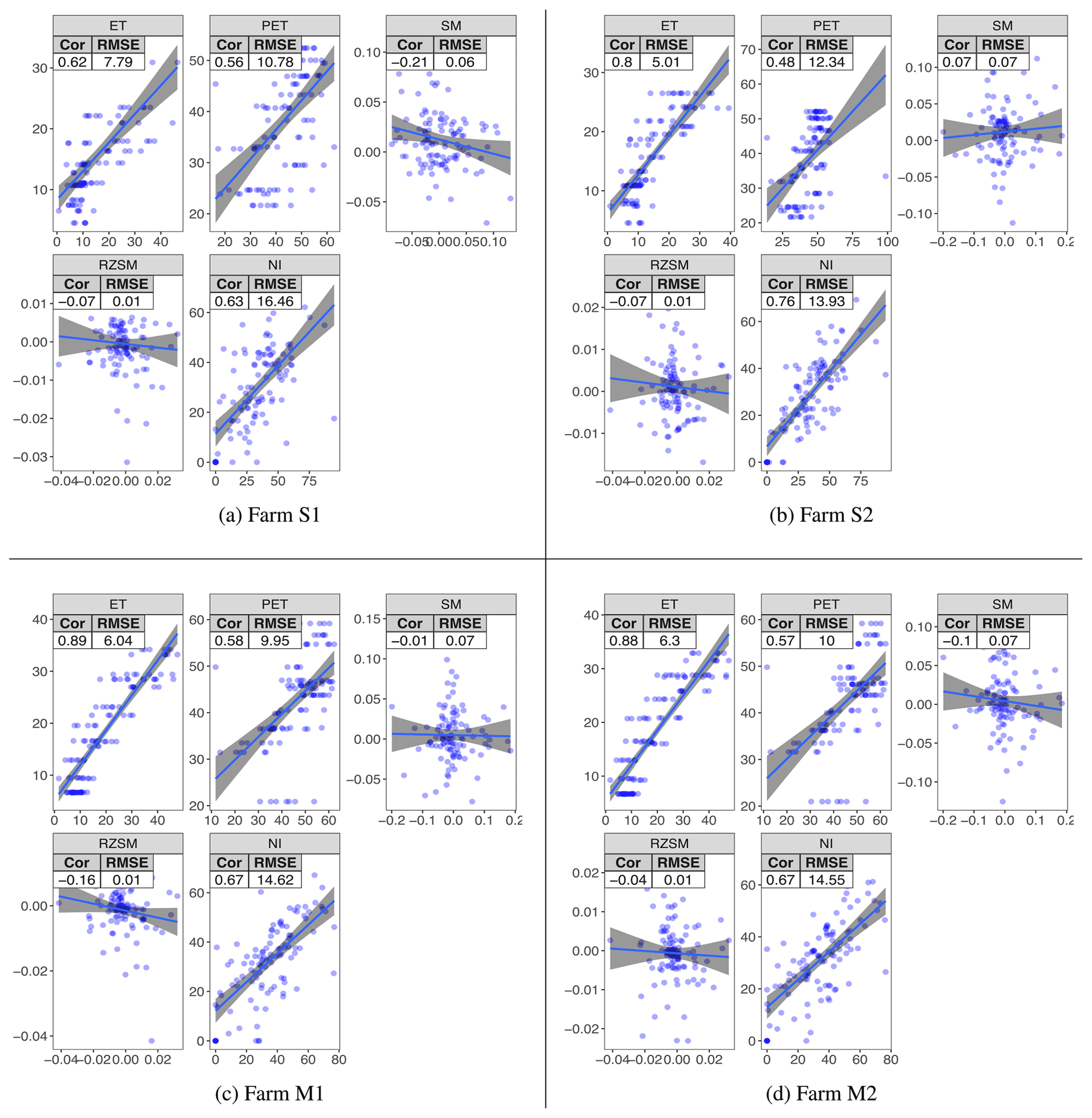
Figure 9The 8 d correlation and RMSE plots for agricultural periods of Farms S1, S2, M1, and M2 (2015–2020). Horizontal axes show observed values. Vertical axes are predicted. Note that the predicted NI is indirectly calculated from all the predicted variables. The crop is barley for the duration of 150 d of planting each year. Gray shades aid the eye in seeing linear patterns using a lm smoothing function.
Table 5KGE values of different covariates for different farms.
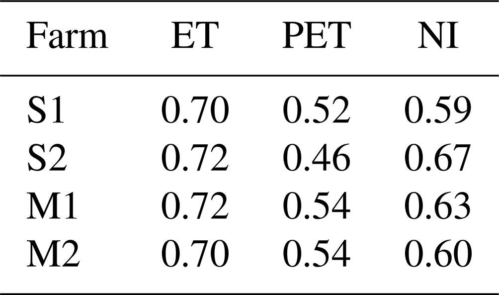
KGE test is the goodness of fit. Generally, values higher than 0.41 are considered reasonable and with a satisfactory model performance, but there has not been a direct reason to choose this benchmark across all models (Knoben et al., 2019). We consider 0.5 ≤ KGE satisfactory in this study. The model's goodness of fit is reasonable for ET, PET, and NI. The KGE values of ΔSM and ΔRZSM (not shown) have been zero or very close to zero. Here, the KGE negative values do not necessarily indicate a model that performed worse than the mean benchmark. The reason is that the range of Δ values of SM and RZSM was relatively small (approx. [−0.87, 0.03] m3 m−3), making the values very sensitive to the statistical tests. For the same reasons, it was expected that ΔSM and ΔRZSM did not show a good correlation, although they showed the lowest RMSE values (Fig. 9). Given the satisfactory performance in final NI calculations, ΔSM and ΔRZSM predictions did not negatively affect the model and NI.
Generally, there is inherent uncertainty in FarmCan forecasts since we cannot know the actual value of the water deficiency and other controlling factors that maximize the crop yield. However, despite the unknowns, FarmCan showed an effective prediction capability to improve our understanding of NI and some of its main controlling factors in the CPE.
With the FarmCan model, we can select any number of CPE farms from airborne imagery, retrieve their spaceborne data, and forecast each farm's crop-specific water supply and demand to calculate water deficit. This tool is versatile enough to allow access to any farm's critical hydroclimatic information for the best water-related decision-making without stepping into the farm or setting up expensive monitoring equipment.
In this study, we develop the FarmCan model to bridge the gap between scientific modeling and practical, easy-to-understand water management decisions. FarmCan is a parsimonious supply–demand crop water monitor and forecasting mechanism. We demonstrated the potential of managing the sustainable productivity of the land by the timing and tuning of water available to the crops. The algorithm used NASA's NRT remote sensing data representing both atmospheric and soil properties coupled with the farm-specific information, water balance, and ML information to generate crop NI up to 14 d in advance, as well as the historical graphs for the farm.
For daily predictions, we used RF using 3-week data from 1 week prior, the current week, and 1 week over, and the data from the same days in the past years. This functionality allowed the FarmCan algorithm to take care of the seasonal variability automatically. In the next step, FarmCan will use the MSWX product, which enables this tool to function in real time and as a prediction tool.
We showed the relative importance of ET and SM in understanding the predictive value of NI in the CPE. Compared to the daily data, we found that 8 d composite variables are stronger calculators for predicting NI as the 8 d tempers the inherent lags associated with P, soil, and atmospheric demand interactions. In addition, the phenological stage of the crop had a determinant factor in using ΔSM or ΔRZSM in the model.
In all four study farms, RF was effectively applied to predict the variables. The correlation between observed and predicted 8 d PET showed an average of 54 %, and the 8 d NI forecast showed an average correlation of 68 %. On the other hand, the correlation values between observed and predicted ΔSM or ΔRZSM were almost zero. Given the small range of variability in Δ values, the correlation numbers cannot be indicators of the lack of contribution of soil moisture in the model.
The KGE values of RF predictions for the 8 d ET and 8 d PET showed an average of 0.71 and 0.50, respectively. Overall, FarmCan could forecast 8 d NI for the four farms with an average KGE of 0.62.
We saw a minimal impact on fluxes between ET and SM in the CPE during the agricultural year. We speculate that is due to the climate of the CPE. During the growing season, the condition in CPE is either too wet, which makes the total energy for ET independent of SM, or too dry, which makes ET show little impact on fluxes because it is little or no moisture available. However, more studies are required to understand the feedback between ET and SM in other environments. For example, in transitional environments, we expect to see that the total energy of ET is more dependent on SM.
We quantitatively showed that, in the rainfed farms in the CPE, optimum crop production in the dry season should only be possible with an extra water supply. Crop production in some years may be possible but unreliable. Climate change will further affect this situation, and farmers are encouraged to move toward water management and adaptation strategies. Future studies can focus on such water shortages' social and economic implications (crop loss, reduced yield, and water costs).
Future developments will focus on the role of the water retention capacity of the soil and crop type as two critical factors potentially affecting NI measurements. Plants in sandy soils, for example, may undergo water stress quicker when water is deficient. In contrast, plants in deep clay and fine texture may have ample time to adjust to low moisture conditions and remain unaffected by water deficiencies.
Future developments will also address how farmers can access FarmCan data, how supplementary irrigation vs. rain-only farming can help farm cost/benefit management, and how the NI predictions and management advisory aid in better on-farm water management and crop yield. Coupling the fertilization timing and amount is another direction that can benefit farmers. Receiving feedback data from the farm managers will allow for yield and cost–benefit analyses.
Despite the inherent uncertainty in FarmCan forecasts, FarmCan is a step toward providing knowledge that can assist farm managers in making better decisions about excess water needs, drainage requirements, timing, and fertilizer consumption.
| CLSM | Catchment Land Surface Model |
| ET | Evapotranspiration |
| FAO | Food and Agricultural Organization |
| GEOS | Goddard Earth Observation System |
| LAI | Leaf area index |
| ML | Machine learning |
| MSWEP | Multi-Source Weighted-Ensemble |
| Precipitation | |
| MODIS | Moderate Resolution Imaging |
| Spectroradiometer | |
| NI | Needed irrigation |
| NRT | Near-real time |
| PET | Potential evapotranspiration |
| P | Precipitation |
| RF | Random forest |
| RZSM | Root zone soil moisture |
| SMAP | Soil moisture active passive |
| SM | (Surface) soil moisture |
| WUE | Water use efficiency |
The code that supports the findings of this study has been written by the corresponding author (Sara Sadri) in R and is available upon reasonable request.
Soil moisture data used in this study are from NASA, provided by Ming Pan, and MSWEP data are from Hylke E. Beck. Other data are fully cited with updated URLs and last date of access. Such data are also available from the corresponding author (Sara Sadri).
SS conceptualized the project with EFW, developed the methodology and software, conducted the formal analysis, and wrote the original and final draft. MP collected the resources with HB and edited paper with AB, HB, and JFS. HB provided the resources, edited the paper, and acted as a consultant.
The contact author has declared that none of the authors has any competing interests.
Publisher's note: Copernicus Publications remains neutral with regard to jurisdictional claims in published maps and institutional affiliations.
This article is part of the special issue “Experiments in Hydrology and Hydraulics”. It is not associated with a conference.
We would like to thank all the referees for this article. Their reviews helped to enhance the quality of this article tremendously. We also would like to express our gratitude to Daniel Green, the editor of this article.
This research has been supported by the Global Institute for Water Security, University of Saskatchewan (grant no. 348882).
This paper was edited by Daniel Green and reviewed by Geoff Pegram and 11 anonymous referees.
Al Bitar, A., Mialon, A., Kerr, Y. H., Cabot, F., Richaume, P., Jacquette, E., Quesney, A., Mahmoodi, A., Tarot, S., Parrens, M., Al-Yaari, A., Pellarin, T., Rodriguez-Fernandez, N., and Wigneron, J.-P.: The global SMOS Level 3 daily soil moisture and brightness temperature maps, Earth Syst. Sci. Data, 9, 293–315, https://doi.org/10.5194/essd-9-293-2017, 2017. a
Allen, R. G., Pereira, L. S., Raes, D., and Smith, M.: Crop evapotranspiration – Guidelines for computing crop water requirements, FAO Irrigation and drainage paper 56, FAO, Rome, Italy, http://www.fao.org/3/X0490E/X0490E00.htm (last access: October 2022), 1998. a
Allen, R., Tasumi, M., and Trezza, R.: Satellite-based energy balance for mapping evapotranspiration with internalized calibration (METRIC)-Model, J. Irrig. Drain. Eng., 133, 380–394, 2007. a
Andarzian, B., Bannayan, M., Steduto, P., Mazraeh, H., Barati, M., Barati, M., and Rahnama, A.: Validation and testing of the AquaCrop model under full and deficit irrigated wheat production in Iran, Agr. Water Manage., 100, 1–8, https://doi.org/10.1016/j.agwat.2011.08.023, 2011. a
Ash, G. H. B., Shaykewich, C. F., and Raddatz, R. L.: Moisture risk assessment for spring wheat on the eastern Prairies: a water use simulation model, Climatol. Bull., 26, 65–78, 1992. a
Beck, H., Wood, E., Pan, M., Fisher, C., van Dijk, D. M. A., and Adler, T. M. R.: MSWEP V2 global 3-hourly 0.1 precipitation: methodology and quantitative assessment, B. Am. Meteorol. Soc., 0, 473–500, 2019. a, b, c, d
Beck, H. E., van Dijk, A. I. J. M., Larraondo, P. R., McVicar, T. R., Pan, M., Dutra, E., and Miralles, D. G.: MSWX: Global 3-hourly 0.1 bias-corrected meteorological data including near-real-time updates and forecasted ensembles, B. Am. Meteorol. Soc., 103, E701–E732, 2022. a
Bhuiyan, H. A., McNairn, H., Powers, J., Friesen, M., Pacheco, A., Jackson, T. J., Cosh, M. H., Colliander, A., Berg, A., Rowlandson, T., Bullock, P., and Magagi, R.: Assessing SMAP Soil Moisture Scaling and Retrieval in the Carman (Canada) Study Site, Vadose Zone J., 17, 1–14, 2018. a
Bonsal, B. R., Zhang, X., and Hogg, W. D.: Canadian Prairie growing season precipitationvariability and associated atmospheric circulation, Clim. Res., 11, 191–208, 1999. a
Breiman, L.: Random forests, Mach. Learn., 45, 5–32, 2001. a
Brouwer, C. and Heibloem, M.: Irrigation Water Management: Irrigation Water Needs, Training manual no. 3, Food and Agriculture Organization of the United Nations, Rome, Italy, http://www.fao.org/3/s2022e/s2022e00.htm#Contents (last access: October 2022), 1986. a
Brust, C., Kimball, J. S., Maneta, M. P., Jencso1, K., and Reichle, R. H.: DroughtCast: A Machine Learning Forecast of the United States Drought Monitor, Front. Big Data, 4, 1–16, https://doi.org/10.3389/fdata.2021.773478, 2021. a, b
Chalmers, D., Mitchell, P., and Heek, L. V.: Control of peach tree growth and productivity by regulated water supply, tree density, and summer pruning [Trickle irrigation], J. Am. Soc. Hortic. Sci., 106, 307–312, 1981. a
Chen, L. and Dirmeyer, P.: Impacts of land-use/land-cover change on afternoon precipitation over North America, J. Climate, 30, 2121–2140, 2017. a
Cherneski, P.: The Impacts and Costs of Drought to the Canadian Agriculture Sector, Saskatchewan, Canada, https://www.drought.gov/nadm/sites/drought.gov.nadm/files/activities/2018Workshop/8_3_CHERNESKI-Agricultural_Drought_Impacts_Canada.pdf (last access: October 2022), 2018. a
Clewley, D., Whitecomb, J., Akbar, R., Silva, A., Berg, A., Adams, J., Caldwell, T., and coauthors: A Method for Upscaling In Situ Soil Moisture Measurements to Satellite Footprint Scale Using Random Forests, IEEE J. Select. Top. Appl. Earth Obs. Remote Sens., 10, 2663–2673, 2017. a
ECCC: Annual Crop Inventory, https://open.canada.ca/data/en/dataset/ba2645d5-4458-414d-b196-6303ac06c1c9 (last access: October 2022), 2013. a
Entekhabi, D., Das, N., Njoku, E., Yueh, S., Johnson, J., and Shi, J.: Algorithm Theoretical Basis Document L2 & L3 Radar/Radiometer Soil Moisture (Active/Passive) Data Products, Document, JPL, 2014. a
Famiglietti, J. S. and Wood, E. F.: Multiscale modeling of spatially variable water and energy balance process, Water Resour. Res., 30, 3061–3078, 1994. a
FAO: How to Feed the World in 2050, http://www.fao.org/fileadmin/templates/wsfs/docs/expert_paper/How_to_Feed_the_World_in_2050.pdf (last access: October 2022), 2009. a
Fisher, J., Melton, F., Middleton, E., Hain, C., Anderson, M., Allen, R., McCabe, M. F., Hook, S., Baldocchi, D., Townsend, P. A., Kilic, A., Tu, K., Miralles, D. D., Perret, J., Lagouarde, J., Waliser, D., Purdy, A. J., French, A., Schimel, D., Famiglietti, J. S., Stephens, G., and Wood, E. F.: The future of evapotranspiration: Global requirements for ecosystem functioning, carbon and climate feedbacks, agricultural management, and water resources, Water Resour. Res., 53, 2618–2626, 2017. a
Franz, T., Heeren, D., Pokal, S., Gholizadeh, H., Rudnick, D., Jin, Z., Tenorio, F., Zhou, Y., Gibson, J., Gates, J., McCabe, M., Guan, K., Ziliani, M., Pan, M., and Wardlow, B.: The role of topography, soil, and remotely sensed vegetation condition towards predicting crop yield, Field Crops Res., 252, 107788, https://doi.org/10.1016/J.Fcr.2020.107788, 2020. a
Geerts, S. and Raes, D.: Deficit irrigation as an on-farm strategy to maximize crop water productivity in dry areas, Agr. Water Manage., 96, 1275–1284, 2009. a
Hadwen, T. and Schaan, G.: The 2017 Drought in the Canadian Prairies, Report, Agriculture Agrifood Canada, https://www.preventionweb.net/files/78461_cs4.gar2017canadianprairiesdroughtc.pdf (last access: September 2021), 2017. a
Han, M., Zhang, H., DeJonge, K. C., Comas, L. H., and Gleason, S.: Comparison of three crop water stress index models with sap flow measurements in maize, Agr. Water Manage., 203, 366–375, 2018. a, b
Jia, Y., Shen, S., Niu, C., Qiu, Y., Wang, H., and Liu, Y.: Coupling crop growth and hydrologic models to predict crop yield with spatial analysis technologies, J. Appl. Remote Sens., 5, 1–20, 2011. a
Kirda, C.: Deficit Irrigation Practices – Deficit irrigation scheduling based on plant growth stages showing water stress tolerance, Report 22, Cukuroya University, Rome, Italy, https://www.fao.org/3/y3655e/y3655e00.htm#TopOfPage (last access: October 2022), 2000. a
Knoben, W. J. M., Freer, J. E., and Woods, R. A.: Technical note: Inherent benchmark or not? Comparing Nash–Sutcliffe and Kling–Gupta efficiency scores, Hydrol. Earth Syst. Sci., 23, 4323–4331, https://doi.org/10.5194/hess-23-4323-2019, 2019. a
Koster, R., Guo, Z., Yang, R., Dirmeyer, P., Mitchell, K., and Pum, M.: On the nature of soil moisture in land surface models, J. Climate, 22, 4322–4335, 2009. a
Levidowa, L., Zaccariab, D., Maiac, R., Vivasc, E., Todorovicd, M., and Scardigno, A.: Improving water-efficient irrigation: Prospects and difficulties of innovative practices, Agr. Water Manage., 146, 84–94, 2014. a, b
Liu, Q., Reichle, R. H., Bindlish, R., Cosh, M. H., Crow, W. T., de Jeu, R., Lannoy, G. J. M. D., Huffman, G. ., and Jackson, T. J.: The contributions of precipitation and soil moisture observations to the skill of soil moisture estimates in a land data assimilation system, J. Hydrometeorol., 12, 750–765, 2011. a
Loggenberg, K., Strever, A., Greyling, B., and Poona, N.: Modelling water stress in a Shiraz Vineyard using hyperspectral imaging and machine learning, Remote Sens., 10, 1–14, https://doi.org/10.3390/rs10020202, 2018. a
Martens, B., Miralles, D. G., Lievens, H., van der Schalie, R., de Jeu, R. A. M., Fernández-Prieto, D., Beck, H. E., Dorigo, W. A., and Verhoest, N. E. C.: GLEAM v3: satellite-based land evaporation and root-zone soil moisture, Geosci. Model Dev., 10, 1903–1925, https://doi.org/10.5194/gmd-10-1903-2017, 2017. a
Maybank, J., Bonsal, B., Jones, K., Lawford, R., O'Brien, E., Ripley, E., and Wheaton, E.: Drought as a natural disaster, Atmos.-Ocean, 33, 195–222, 1995. a
McGinn, S. and Shepherd, A.: Impact of climate change scenarios on the agroclimate of the Canadian prairies, Can. J. Soil Sci., 83, 623–630, 2003. a
Papagiannopoulou, C., Miralles, W. D., Verhoest, N., Depoorter, M., and Waegeman, W.: Vegetation anomalies caused by antecedent precipitation in most of the world, Environ. Res. Lett., 12, 074016, https://doi.org/10.1088/1748-9326/aa7145, 2017. a
Pendergrass, A. G., Meehl, G. A., Pulwarty, R., Hobbins, M., Hoell, A., AghaKouchak, A., Bonfils, C. J. W., Gallant, A. J. E., Hoerling, M., Hoffmann, D., Kaatz, L., Lehner, F., Llewellyn, D., Mote, P., Neale, R. B., Overpeck, J. T., Sheffield, A., Stahl, K., Svoboda, M., Wheeler, M. C., Wood, A. W., and Woodhouse, C. A.: Flash droughts present a new challenge for subseasonal-to-seasonal prediction, Nat. Clim. Change, 10, 191–199, https://doi.org/10.1038/s41558-020-0709-0, 2020. a
Pereira, L. S., Allen, R. G., Smith, M., and Raes, D.: Crop evapotranspiration estimation with FAO56: Past and future, Agr. Water Manage., 147, 4–20, https://doi.org/10.1016/j.agwat.2014.07.031, 2015. a, b, c
Poblete, T., Ortega-Farias, S., and Bardeen, M. M. M.: Artificial neural network to predict vine water status spatial variability using multispectral information obtained from an unmanned aerial vehicle (UAV), Sensors, 17, 2488, https://doi.org/10.3390/s17112488, 2017. a
Poccas, I., Gonccalves, J., Costa, P., Gonccalves, I., Pereira, L., and Cunha, M.: Hyperspectral-based predictive modelling of grapevine water status in the portuguese douro wine region, Int. J. Applied Earth Obs. Geoinf., 58, 177–190, 2017. a
Pomeroy, J., Nicholaichuk, W., Cray, D., McConkey, B., Cranger, R., and Landine, P.: Snow Management And Meltwater Enhancement, Final Report, Tech. Report CS-90021, Nationl Hydrology Research Institute, Environment Canada, Sasiatoon, Saskatchewan, http://citeseerx.ist.psu.edu/viewdoc/download?doi=10.1.1.725.7817&rep=rep1&type=pdf (last access: September 2021), 1990. a
Quiring, S.: Growing-season moisture variability in the eastern USA during the last 800 years, Clim. Res., 27, 9–17, 2004. a
Rapaport, T., Hochberg, U., Shoshany, M., Karnieli, A., and Rachmilevitch, S.: Combining leaf physiology, hyperspectral imaging and partial least squares-regression (PLS-R) for grapevine water status assessment, ISPRS J. Photogram. Remote Sens., 109, 88–97, 2015. a
Reichle, R., Lucchesi, R., Ardizzone, J. V., Kim, G., Smith, E. B., and Weiss, B. H.: Soil Moisture Active Passive (SMAP) Mission Level 4 Surface and Root Zone Soil Moisture (L4SM) Product Specification Document, Tech. Rep. 10 (Version 1.4), NASA Goddard Space Flight Center, Greenbelt, MD, https://ntrs.nasa.gov/api/citations/20190001102/downloads/20190001102.pdf (last access: October 2022), 2015. a
Reichle, R. H.: Assessment of the SMAP Level-4 Surface and Root-Zone Soil Moisture Product Using In Situ Measurements, J. Hydrometeorol., 18, 2621–2645, 2017. a
Reichle, R. H., Koster, R. D., Lannoy, G. J. M. D., Forman, B. A., Liu, Q., Mahanama, S. P. P., and Toure, A.: Assessment and enhancement of MERRA land surface hydrology estimates, J. Climate, 24, 6322–6338, 2011. a
Reichle, R. H., Liu, Q., Koster, R. D., Crow, W. T., Lannoy, G. J. M. D., Kimball, J. S., Ardizzone, J. V., Bosch, D., Colliander, A., Cosh, M., Kolassa, J., Mahanama, S. P., Prueger, J., Starks, P., and Walker, J. P.: Version 4 of the SMAP Level-4 Soil Moisture Algorithm and Data Product, J. Adv. Model. Earth Syst., 11, 3106–3130, 2019. a
Rienecker, M., Suarez, M., Todling, R., Bacmeister, J., Takacs, L., Liu, H. C., Gu, W., Sienkiewicz, M., Koster, R., Gelaro, R., Stajner, I., and Nielsen, J.: The GEOS-5 Data Assimilation System – Documentation of Versions 5.0.1, 5.1.0, and 5.2.0, NASA Technical Report Series on Global Modeling and Data Assimilation, NASA/TM-2008-104606, vol. 28, NASA, 101 pp., https://ntrs.nasa.gov/api/citations/20120011955/downloads/20120011955.pdf (last access: October 2022), 2008. a
Romero, M., Luo, Y., Su, B., and Fentes, S.: Vineyard water status estimation using multispectral imagery from an UAV platform and machine learning algorithms for irrigation scheduling management, Comput. Elect. Agricult., 147, 109–117, 2018. a
Running, S. W., Mu, Q., Zhao, M., and Moreno, A.: User's Guide MODIS Global Terrestrial Evapotranspiration (ET) Product (MOD16A2/A3 and Year-end Gap-filled MOD16A2GF/A3GF) NASA Earth Observing System MODIS Land Algorithm (For Collection 6), LP DAAC, https://lpdaac.usgs.gov/documents/600/MOD16GF_vs_NTSG.pdf (last access: October 2020), 2019a. a
Running, S., Mu, Q., Zhao, M., and Moreno, A.: MOD16A3GF MODIS/Terra Net Evapotranspiration Gap-Filled Yearly L4 Global 500 m SIN Grid V006, NASA EOSDIS Land Processes DAAC [data set], https://doi.org/10.5067/MODIS/MOD16A3GF.006, 2019b. a, b, c, d
Sadri, S., Wood, E. F., and Pan, M.: Developing a drought-monitoring index for the contiguous US using SMAP, Hydrol. Earth Syst. Sci., 22, 6611–6626, https://doi.org/10.5194/hess-22-6611-2018, 2018. a
Sadri, S., Pan, M., Wada, Y., Vergopolana, N., Sheffield, J., Famigliettie, J. S., Kerr, Y., and Wood, E.: A global near-real-time soil moisture index monitor for food security using integrated SMOS and SMAP, Remote Sens. Environ, 246, 1–22, 2020. a, b, c
Saini, R. and Ghosh, S.: Crop classification on single date sentinel-2 imagery using random forest and support vector machine, International Archives of the Photogrammetry, Remote Sensing and Spatial Information Sciences, XLII, 683–688, 2018. a
Saskatchewan Government: Irrigation Development Process, https://www.saskatchewan.ca/business/agriculture-natural-resources-and-industry/agribusiness-farmers-and-ranchers/crops-and-irrigation/irrigation/irrigation-development-process (last access: October 2022), 2022. a
ScienceDaily: Scientists propose improvements to precision crop irrigation, University of Illinois, College of Agricultural, Consumer and Environmental Sciences, https://www.sciencedaily.com/releases/2021/04/210429112359.htm, last access: 2 September 2021. a
Seneviratne, S. I., Corti, T., Davin, E. L., Hirschi, M., Jaeger, E. B., Lehner, I., Orlowsky, B., and Teuling, A. J.: Investigating soil moisture–climate interactions in a changing climate: A review, Earth-Sci. Rev., 99, 125–161, 2010. a, b
Shuval, H. and Dweik, H.: Water Resources in the Middle East, Israel-Palestinian Water Issues – From Conflict to Cooperation, vol. 2, Springer, Jerusalem, Israel, p. 80, 136, ISBN 978-3-540-69508-0, https://doi.org/10.1007/978-3-540-69509-7, 2007. a
Smilovic, M., Gleeson, T., and Adamowski, J.: Crop kites: Determining crop-water production functions using crop coefficients and sensitivity indices, Adv. Water Resour., 97, 193–204, 2016. a
Smilovic, M., Gleeson, T., Adamowski, J., and Langhorn, C.: More food with less water-Optimizing agricultural water use, Adv. Water Resour., 123, 256–261, 2019. a
Sonth, M. V., Ambesange, S., Sreekanth, D., and Tulluri, S.: Optimization of Random Forest Algorithm with Ensemble and Hyper Parameter Tuning Techniques for Multiple Heart Diseases, Solid State Technology, 63 pp., https://doi.org/10.13140/RG.2.2.12451.68649, 2020. a
Stocker, T. F., Qin, D., Tignor, M., Allen, S. K., Boschung, J., Nauels, A., Xia, Y., Bex, V., and Midgley, P.: Climate Change 2013 – The Physical Science Basis: Working Group I Contribution to the Fifth Assessment Report of the Intergovernmental Panel on Climate Change, Cambridge University Press, Cambridge, UK and New York, NY, USA, ISBN 978-1-107-66182-0, 2013. a
Taghvaeian, S., Andales, A. A., Allen, L. N., Kisekka, I., O'Shaughnessy, S. A., Porter, D. O., Sui, R., Irmak, S., Fulton, A., and Aguilar, J.: Irrigation Scheduling for Agriculture in the United States: The Progress Made and the Path Forward, T. ASABE, 63, 1603–1618, 2020. a, b, c, d, e
Tetlock, E., Toth, B., Berg, A., Rowlandson, T., and Ambadan, J. T.: An 11-year (2007–2017) soil moisture and precipitation dataset from the Kenaston Network in the Brightwater Creek basin, Saskatchewan, Canada, Earth Syst. Sci. Data, 11, 787–796, https://doi.org/10.5194/essd-11-787-2019, 2019. a, b
UN/ISDR: Drought Risk Reduction Framework and Practices: Contributing to the Implementation of the Hyogo Framework for Action, Tech. Rep. 98+vi pp., UN/ISDR – United Nations Secretariat of the International Strategy for Disaster Reduction, Geneva, Switzerland, https://www.unisdr.org/files/3608_droughtriskreduction.pdf (last access: October 2022), 2007. a
USDA-NASS: Irrigation and Water Management Survey, Washington, DC, https://www.nass.usda.gov/Surveys/Guide_to_NASS_Surveys/Farm_and_Ranch_Irrigation/index.php (last access: October 2022), 2021. a, b
Vergopolan, N., Xiong, S., Estes, L., Wanders, N., Chaney, N. W., Wood, E. F., Konar, M., Caylor, K., Beck, H. E., Gatti, N., Evans, T., and Sheffield, J.: Field-scale soil moisture bridges the spatial-scale gap between drought monitoring and agricultural yields, Hydrol. Earth Syst. Sci., 25, 1827–1847, https://doi.org/10.5194/hess-25-1827-2021, 2021. a, b, c
Virnodkar, S. S., Pachghare, V. K., Patil, V. C., and Jha, S. K.: Remote sensing and machine learning for crop water stress determination in various crops: a critical review, Precis. Agric., 21, 1121–1155, 2020. a, b, c, d, e, f
Wanders, N., Karssenberg, D., de Roo, A., de Jong, S. M., and Bierkens, M. F. P.: The suitability of remotely sensed soil moisture for improving operational flood forecasting, Hydrol. Earth Syst. Sci., 18, 2343–2357, https://doi.org/10.5194/hess-18-2343-2014, 2014. a
Wheaton, E., Wittrock, V., Kulshreshtha, S., Koshida, G., Chipanshi, A., and Bonsal, B.: Lessons Learned from the Canadian Drought Years of 2001 and 2002: Synthesis Report for Agriculture and Agri-Food Canada, Tech. Rep. SRC publication no. 11602-46E03, Saskatoon, Saskatchewan Research Council, Saskatoon, https://agriculture.canada.ca/en/agriculture-and-environment/drought-watch-and-agroclimate/managing-agroclimate-risk/lessons-learned-canadian-drought-years-2001-and-2002 (last access: October 2022), 2005. a, b
White, J., Berga, A. A., Champagneb, C., Zhangb, Y., Chipanshi, A., and Daneshfar, B.: Improving crop yield forecasts with satellite-based soil moisture estimates: An example for township level canola yield forecasts over the Canadian Prairies, Int. J. Appl. Earth Obs. Geoinf., 89, 1–12, 2020. a, b, c
Wittrock, V. and Ripley, E.: The predictability of autumn soil moisture levels on the Canadian Prairies, J. Climatol., 19, 271–289, 1999. a
Yang, Y., Donohue, R., and McVicar, T.: Global estimation of effective plants rooting depth: Implications for hydrological modeling, Water Resour. Res., 52, 8260–8276, 2016. a
Yang, Y., Guan, K., Zhang, J., Peng, B., Pan, M., and Zhou, W.: Incorporating a plant water supply-demand faramework into Noah-MP land surface model to simulate hydrological fluxes for agroecosystems, in: American Geophysical Union Fall Meeting, San Francisco, B046-0018, 2020. a, b, c
Zohaib, M., Kim, H., and Choi, M.: Evaluating the patterns of spatiotemporal trends of root zone soil moisture in major climate regions in East Asia, J. Geophys. Res.-Atmos., 122, 7705–7722, 2017. a