Attribution of climate change and human activities to streamflow variations with a posterior distribution of hydrological simulations

Hydrological simulations are a main method of quantifying the contribution rate (CR) of climate change (CC) and human activities (HAs) to watershed streamflow changes. However, the uncertainty of hydrological simulations is rarely considered in current research. To fill this research gap, based on the Soil and Water Assessment Tool (SWAT) model, in this study, we propose a new framework to quantify the CR of CC and HAs based on the posterior histogram distribution of hydrological simulations. In our new quantitative framework, the uncertainty of hydrological simulations is first considered to quantify the impact of “equifinality for different parameters”, which is common in hydrological simulations. The Lancang River (LR) basin in China, which has been greatly affected by HAs in the past 2 decades, is then selected as the study area. The global gridded monthly sectoral water use data set (GMSWU), coupled with the dead capacity data of the large reservoirs within the LR basin and the Budyko hypothesis framework, is used to compare the calculation result of the novel framework. The results show that (1) the annual streamflow at Yunjinghong station in the Lancang River basin changed abruptly in 2005, which was mainly due to the construction of the Xiaowan hydropower station that started in October 2004. The annual streamflow and annual mean temperature time series from 1961 to 2015 in the LR basin showed significant decreasing and increasing trends at the α= 0.01 significance level, respectively. The annual precipitation showed an insignificant decreasing trend. (2) The results of quantitative analysis using the new framework showed that the reason for the decrease in the streamflow at Yunjinghong station was 42.6 % due to CC, and the remaining 57.4 % was due to HAs, such as the construction of hydropower stations within the study area. (3) The comparison with the other two methods showed that the CR of CC calculated by the Budyko framework and the GMSWU data was 37.2 % and 42.5 %, respectively, and the errors of the calculations of the new framework proposed in this study were within 5 %. Therefore, the newly proposed framework, which considers the uncertainty of hydrological simulations, can accurately quantify the CR of CC and HAs to streamflow changes. (4) The quantitative results calculated by using the simulation results with the largest Nash–Sutcliffe efficiency coefficient (NSE) indicated that CC was the dominant factor in streamflow reduction, which was in opposition to the calculation results of our new framework. In other words, our novel framework could effectively solve the calculation errors caused by the “equifinality for different parameters” of hydrological simulations. (5) The results of this case study also showed that the reduction in the streamflow in June and November was mainly caused by decreased precipitation and increased evapotranspiration, while the changes in the streamflow in other months were mainly due to HAs such as the regulation of the constructed reservoirs. In general, the novel quantitative framework that considers the uncertainty of hydrological simulations presented in this study has validated an efficient alternative for quantifying the CR of CC and HAs to streamflow changes.

1 Introduction

The hydrological cycle of the watershed and water resource systems is deeply influenced by climate change (CC) and human activities (HAs) (Bao et al., 2012; Chandesris et al., 2019; Han et al., 2019; Teuling et al., 2019). CC mainly refers to changes in precipitation and evapotranspiration that are caused by rising temperatures and water vapor (Hegerl et al., 2015), while the impact of HAs is mainly reflected in the following aspects: reservoir construction changes the spatial and temporal distribution of streamflow processes (Hennig et al., 2013; Chandesris et al., 2019), land use changes change the characteristics of the underlying surface of the watershed, in turn affecting the streamflow of the watershed (Yang et al., 2017), and population increase leads to an increase in the amount of water used for domestic consumption (Teuling et al., 2019). However, identifying which CC and HAs are the main factors driving the changes in the water cycle of river basins is of great significance for water resource managers to formulate policies for sustainable water resource utilization (Dey and Mishra, 2017; Liu et al., 2017). If CC is the dominant driving factor, then hydrometeorologists need to assess the future trends of meteorological factors, such as precipitation and temperature, to change their water resource management strategies in a timely manner. Conversely, if HAs are the dominant factor, water resource managers should evaluate whether the impact of these HAs exceeds the local water resource carrying capacity and then adjust their related policies (Fu et al., 2004).

Numerous published articles have focused on how to quantify the CR of CC and HAs to the streamflow change in river basins (Liu et al., 2019; Bao et al., 2012; Chandesris et al., 2019; Han et al., 2019; Kong et al., 2016; Xie et al., 2019). In general, the commonly used methods of attribution analysis can be divided into the following three categories: (1) conceptual methods, such as the Budyko framework (Li et al., 2007; Liu et al., 2017), (2) hydrological simulation methods (Liu et al., 2019), and (3) analytical methods, such as the climate elasticity method (Liang et al., 2013). What these three methods have in common is that they all need to first test the annual streamflow sequence through nonstationary testing methods (such as the Mann–Kendall test) and then divide the study period into the natural period (before the break point) and the impacted period (after the break point). The first type of method needs to first calculate the sensitivity of the basin's precipitation and potential evapotranspiration to hydrological variables, and then the hydrological changes caused by CC can be calculated combined with the hydrological sensitivity parameters through the changes in precipitation and potential evapotranspiration in the impacted period and natural period so that the CR of HAs is obtained based on the water balance equation (Li et al., 2007). The second type of method simulates multiple scenarios by changing one impact factor with other fixed factors to evaluate the CR of the changed factor using lumped or distributed hydrological models (Liu et al., 2019). The core of these methods is the modeling of two situations where only one impact factor state has been changed, and the difference between the two simulation results is regarded as the influence of the changed factor. The third type of method is mostly based on numerical calculation, taking the climate elasticity method as an example (Liang et al., 2013): this method introduces the concept of climate elasticity to define the quantitative relationship between changes in streamflow and climatic variables (precipitation, evapotranspiration, etc.), and the CR of HAs to streamflow changes can be obtained by subtracting the CR of climate variables. Among the three types of methods, the second types of methods are the most widely used because it has the following advantages: (1) relatively small data requirements (one only needs to input the meteorological and hydrological data to the hydrological model), (2) relatively simple theoretical assumptions, and (3) quantifying the CR of CC and HAs to streamflow changes at the monthly scale.

Various related published articles are briefly reviewed as follows. Bao et al. (2012) used the variable infiltration capacity (VIC) model to investigate the impacts of CC and HAs on streamflow changes in the Haihe River basin, China, and they concluded that HA accounted for more than 70 % of the decrease in streamflow at Guantai station. Wang et al. (2013) used a two-parameter hydrological model to quantify the contribution of CC and HAs to streamflow changes in three river basins (i.e., Zhanghe, Chaohe, and Hutuo River), and they found that HAs were the dominant factor in streamflow changes. The above literature review shows that these studies all used hydrological simulations with fixed parameter sets to quantify the impact of CC and HAs. As pointed out by Abbaspour et al. (2004) and Zhao et al. (2018a), there is a phenomenon of “equifinality for different parameters” (Beven, 2006) in hydrological calibration and simulation, which also means that we cannot ignore the uncertainty of model parameters in the process of quantifying the CR of CC and HAs to streamflow changes because two sets of parameters with the same performance (with the same Nash–Sutcliffe efficiency coefficient) may lead to very different results; this will further influence the decision-making of water resource managers in making effective and sustainable water resource utilization policies. In the last few decades, great progress has been made in evaluating the uncertainty of hydrological simulations (Abbaspour et al., 2004; Beven and Binley, 1992; Yang et al., 2008; Zhao et al., 2018a; Farsi and Mahjouri, 2019); however, in studies related to quantifying the CR of CC and HAs for streamflow changes, few studies have considered the uncertainty of hydrological simulations (Farsi and Mahjouri, 2019). According to our literature search, Farsi and Mahjouri (2019) first considered the uncertainty of hydrological simulations in the process of quantifying the CR of CC and HAs to streamflow changes, but they only constructed the posterior distribution of the CRs of CC and HAs; in their research, they did not specify how to calculate the CRs of CC and HAs while considering the uncertainty of hydrological simulations. Therefore, to fill this research gap, in this study we propose a new method to quantify the contribution of CC and HAs to streamflow changes considering the uncertainty of hydrological simulations, which in summary is developed using the posterior histogram distribution of hydrological simulations.

The Lancang River (LR) is located in Southwest China and is the largest transboundary river in the Indo-China Peninsula; it is usually called the Mekong River (MR) after flowing out of China (Grumbine and Xu, 2011). The abundant water and ecological diversity of the Lancang–Mekong River basin nurtures tens of millions of people in many countries along the Lancang–Mekong River. The upstream flow of the river provides guarantees for irrigation and fishery water use in the countries along the MR during the dry season, and the water conservancy facilities of the LR during the peak of the flood period also provide important engineering guarantees for downstream flood control (Piman et al., 2012, 2016). In the past 3 decades, a series of hydropower stations have been constructed in the LR basin to meet the flood control and drought relief requirements of downstream countries and the power needs of Southwest China. Therefore, it is particularly important to quantify the CR of CC and HAs to streamflow changes in the LR basin. However, so far, there are still few corresponding studies. Han et al. (2019) chose the LR basin as the study area and then divided the research period into three periods, the natural period, transition period, and impacted period, and combined them with the construction time of six large hydropower stations in the LR area. Finally, they found that the CR of HAs during the impact period exceeded 95 %, using the coupled routing and excess storage (CREST) model, which was probably due to the construction of the Nuozhadu hydropower station. However, there are still areas for improvement in their research: (1) the results of the hydrological simulation were relatively poor (with monthly NSE = 0.57 for the whole study period) and (2) the uncertainty involved in hydrological simulations was not considered.

In this paper, the break point of the change in flow regimes was identified using the Mann–Kendall break point test. Then, the study period was divided into a natural period (before the break point) and an impacted period (after the break point). The Soil and Water Assessment Tool (SWAT) model was used for monthly streamflow simulation at Yunjinghong station. Next, the monthly SWAT model was calibrated and validated using the sequential uncertainty fitting procedure version 2 (SUFI-2) (Abbaspour et al., 2004). Uncertainty analysis was also conducted with the SUFI-2 method, and then the posterior histogram frequency distribution (HFD) of the CR of CC and HAs was obtained. Finally, the proposed quantification framework was compared with two other methods: one was the Budyko framework, and the other was to use the LR basin's gridded monthly sectoral water withdrawals in the period from 1971 to 2010 (Huang et al., 2018) together with the dead reservoir storage capacity data of the six constructed hydropower stations along the mainstream of LR to separate the CR of HAs.

2 Study area and data sets

2.1 Study area

The Lancang River (LR) originates in the northeastern Tanggula Mountains, Qinghai Province, China, and flows through China's Qinghai Province, Tibet Autonomous Region and Yunnan Province. It is the largest international river in Southeast Asia, and it is called the Mekong River after it flows out of China. Its mainstream has a total length of ∼ 2161 km and a total catchment area of ∼ 160 000 km² (Han et al., 2019; D. Li et al., 2017). The topography of the LR is characterized by high northern and low southern portions; the maximum elevation in the northern mountainous area can reach ∼ 5871 m, while the lowest elevation in the downstream area is only ∼ 547 m (Fig. 1). This steep terrain difference also leads to the LR having a large potential for hydropower resources. During the past few decades, Huaneng Lancangjiang Hydropower Co., Ltd. constructed six large hydropower stations (i.e., Gongguoqiao, Xiaowan, Manwan, Dachaoshan, Nuozhadu, and Jinghong) on the mainstream of the LR to meet the demands for power and irrigation water in Southwest China (Fig. 1 and Table 1) (Han et al., 2019; Hennig et al., 2013; Xue et al., 2011). At the same time, the construction of these hydropower stations has greatly reduced the risk of flooding in downstream countries and brought great convenience to using water for downstream agricultural irrigation. Detailed information on the six constructed hydropower stations is outlined in Table 1. These data are mainly collected from https://opendevelopmentmekong.net/topics/hydropower/ (last access: 16 October 2022) as well as from other published related literature (Han et al., 2019; Xue et al., 2011; Hennig et al., 2013; Tilt and Gerkey, 2016).

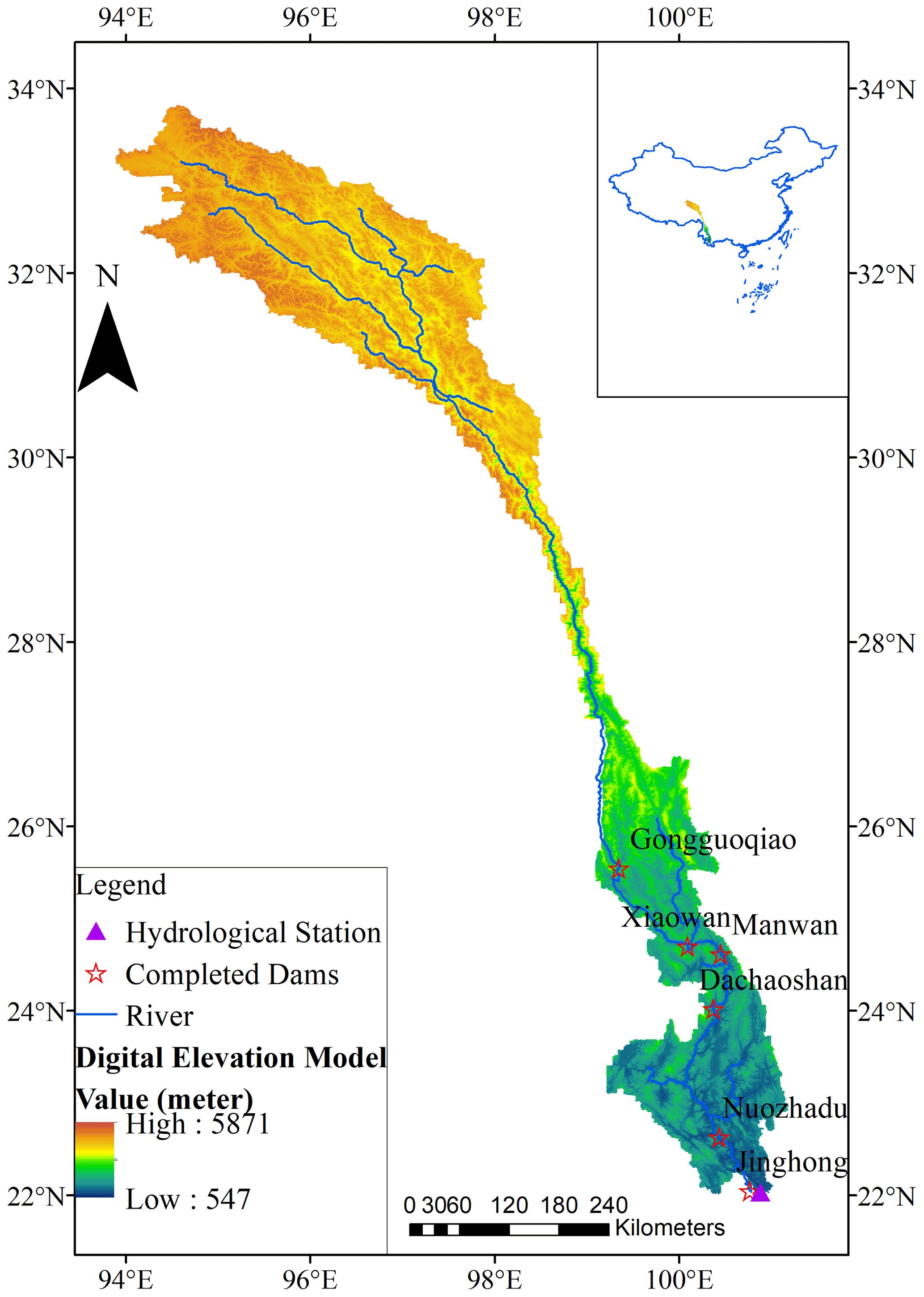
Figure 1 Locations of the Lancang River (LR) basin, Yunjinghong hydrological station, constructed dams on the mainstream of the LRB, and main rivers and elevations (m).

Table 1 Basic information for the six large constructed dams on the mainstream of the LR basin.

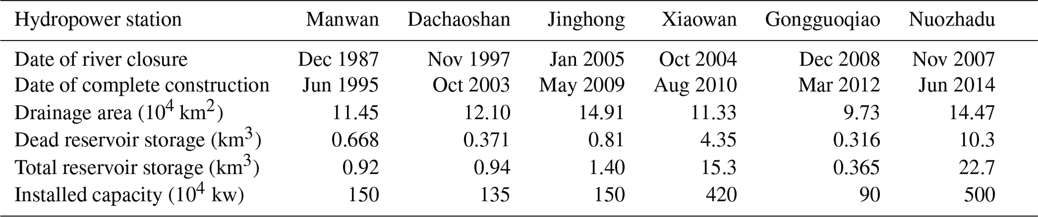
(Notation: dead storage capacity refers to the storage capacity below the dead water level of the reservoir, which does not participate into runoff regulation during the normal operation of the reservoir.)

The LR features an arid climate in the upper mountainous areas, while the lower reaches are dominated by humid climates. The average annual precipitation of the whole basin is ∼ 870 mm based on a 55-year record (from 1961 to 2015) using the China Gauge-based Daily Precipitation Analysis (CGDPA) (Xie et al., 2007; Tang et al., 2019). Due to the influence of the westerlies and the Indian Ocean monsoon, the precipitation in the LR has obvious seasonal changes, and the precipitation from June to September accounts for more than 70 % of the annual precipitation (Jacobs, 2002). Correspondingly, the streamflow of the LR also shows seasonality, and the floods are mostly concentrated from June to September.

2.2 Data sets

The China Gauge-based Daily Precipitation Analysis (CGDPA) product was developed by the China Meteorological Administration (CMA) using data from ∼ 2400 ground-based national weather stations across China (Tang et al., 2018; Xie et al., 2007; Shen et al., 2014). It provides daily precipitation, maximum temperature, minimum temperature, relative humidity, and wind speed data at a 0.25^∘ spatial resolution from 1961 to 2015; this data set can be publicly obtained by contacting its author via email (sheny@cma.gov.cn). Previous studies have successfully applied this product to multiple research areas in China (Tang et al., 2019, 2018; Han et al., 2019). The daily streamflow data from Yunjinghong station for the time period from 1961 to 2015 were collected from the Information Center of the Ministry of Water Resources and the local water resources management department.

The digital elevation model (DEM) used in this study was downloaded from NASA's Shuttle Radar Topography Mission (SRTM) database at a spatial resolution of ∼ 90 m (http://srtm.csi.cgiar.org/, last access: 16 October 2022), which was used to generate the watershed boundary, slope, and sub-watershed data in the SWAT model (Arnold et al., 2012a). The Harmonized World Soil Database (version 1.2) (HWSD v1.2) at a spatial resolution of ∼ 1 km was downloaded from the Food and Agriculture Organization of the United Nations, and this data set contains two layers of soil. The land use and cover data with a spatial resolution of ∼ 1 km were collected from the Geospatial Data Cloud (http://www.gscloud.cn/, last access: 16 October 2022). In this study, to analyze the land use change in the LR during the historical period, we collected five periods of land use data in the 1980s, 1990s, 2000s, and 2010 to 2015, and this data set was downloaded from the Geographic Information Monitoring Cloud Platform (http://www.dsac.cn/, last access: 16 October 2022) with a spatial resolution of 30 m. It should be pointed out that this study only used the land use information in 2010 to construct the SWAT hydrological model and did not consider the dynamic changes in land use information in the hydrological simulation.

The global gridded monthly sectoral water use (GMSWU) data set for 1971–2010 was obtained from https://doi.org/10.5281/zenodo.1209296. This data set was developed by Huang et al. (2018), and it provides the global domestic water use, irrigation water use, livestock water use, manufacturing water use, and mining water use with a spatial resolution of 0.5^∘. This data set is used in this study because it is difficult to collect water withdrawal data related to HAs in the LR basin, and this data set has been successfully applied in this basin in other studies (Han et al., 2019). We used this data set here to roughly separate the effects of HAs in the LR. For more technical information about this set of products, the readers can refer to Huang et al. (2018) and Han et al. (2019). Furthermore, detailed information on six large dams in the mainstream of the LR was collected from Open Development Mekong (https://opendevelopmentmekong.net/topics/hydropower/, last access: 16 October 2022) and Huaneng Lancang River Hydropower Inc. It mainly includes the dates when the rivers start to be closed, when these dams were fully put into use, their dead storage capacity, their total storage capacity, and other information.

3 Methodologies

3.1 The novel proposed framework

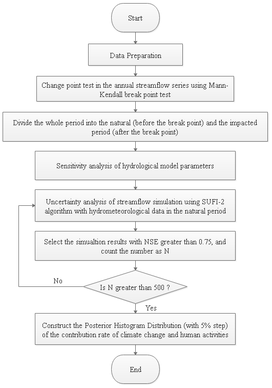
Hydrological simulation is one of the main methodologies to quantify the CR of CC and HAs to streamflow variations; however, in the past, related studies have rarely considered the uncertainty involved in hydrological simulations (Farsi and Mahjouri, 2019). In this section, we will introduce a new quantitative framework to quantify the influence of the common phenomenon of “equifinality for different parameters” in hydrological simulation on the quantitative results by constructing the posterior distribution of streamflow simulations during the implementation process. The specific implementation flowchart is shown in Fig. 2. The detailed execution steps are shown as follows.

• Step 1. Inspection of break points in the annual streamflow sequence; based on the result of the breakpoint test, the entire time series is divided into a natural period (before the break point) and an impacted period (after the break point).

• Step 2. Sensitivity analysis of the parameters in the hydrological model.

• Step 3. According to the results of the parameter sensitivity analysis, selection of the more sensitive parameters and input of the hydrometeorological data of the natural period (before the break point) to calibrate the hydrological model with 1000 runs.

• Step 4. Selection of the parameter sets with Nash–Sutcliffe efficiency (NSE) coefficients greater than 0.75 in 1000 simulations, input of the hydrometeorological data of the impacted period, and further calculation of the CR of CC and HAs to the streamflow change corresponding to each simulation result.

• Step 5. Construction of the posterior histogram distribution (PHD) of the CR of CC and HAs (with a 5 % step), and then the histogram with the highest frequency is treated as the uncertainty CR interval of CC and HAs to the streamflow change.

• The arithmetic mean of the results in the interval is treated as its true CR.

In step 4, to ensure the number of streamflow simulation samples, we set the simulation results with NSE to greater than 0.75 to at least 500 times. If the setting is not met, then step 3 is repeated until the cumulative simulation times are greater than 500 times.

Figure 2 Flowchart of the newly proposed quantitative framework.

3.2 Mann–Kendall test

In this step, the trends and break points of the hydrometeorological data are detected using the nonparametric Mann–Kendall monotonic trend test (Gilbert, 1987; Kendall, 1975; Mann, 1945) and the Mann–Kendall break point test (Sneyers, 1991), respectively. The main consideration of using the Mann–Kendall test is that this method assumes no particular distribution for the tested time series (Song et al., 2019; Xu et al., 2018). Significance levels of α= 0.01 and 0.05 are used in this study.

3.2.1 Mann–Kendall monotonic trend test

The Mann–Kendall (MK) monotonic trend test was developed by Mann (1945), Kendall (1975), and Gilbert (1987), which has been widely used to detect the presence of an upward or downward trend of the hydrometeorological time series, and the advantage of this test is that the time series does not need to follow a certain distribution (Hamed and Ramachandra Rao, 1998). This method first tests whether to reject the null hypothesis (H₀: no monotonic trend) and accept the alternative hypothesis (H_a: with monotonic trend) for a significance level of α. The defined statistic S can be calculated by the following equation:

$$\begin{array}{}\text{(1)}& S=\sum _{k=\mathrm{1}}^{n-\mathrm{1}}\sum _{j=k+\mathrm{1}}^n\mathrm{sign}\left(x_j-x_k,\right),\end{array}$$

where x_k is the data in the order over time, x₁, x₂, …, x_n−1, which means the time series obtained at times 1, 2, …, n−1, respectively. x_j is another time series over time x_k+1, x_k+2, …, x_n. n is the length of the data set record. Sign(x_j−x_k) is a sign function that takes on the values of 1, 0, or -1 based on the sign of x_j−x_k, and its values can be calculated by the following equation:

$$\begin{array}{}\text{(2)}& \mathrm{sign}\left(x_j-x_k\right)=\left\{\begin{array}{l}-\mathrm{1},x_j-x_k<\mathrm{0},\\ \mathrm{0},x_j-x_k=\mathrm{0},\\ \mathrm{1},x_j-x_k>\mathrm{0}.\end{array}\right.\end{array}$$

After calculating the S sequence, the variance of S can be computed as follows:

$$\begin{array}{}\text{(3)}& \begin{array}{rl}& \mathrm{VAR}\left(S\right)\\ & ={\displaystyle \frac{\mathrm{1}}{\mathrm{18}}}\left[n\left(n-\mathrm{1}\right)\left(\mathrm{2}n+\mathrm{5}\right)-\sum _{p-\mathrm{1}}^g{t}_p\left(t_p-\mathrm{1}\right)\left(\mathrm{2}{t}_p+\mathrm{5}\right)\right],\end{array}\end{array}$$

where n is the length of the time series, g is the length of any given tied group, and t_p is the length of the data set series in the pth group. Then, the defined test statistic Z_MK can be transformed from the statistical value S, and the equation is as follows:

$$\begin{array}{}\text{(4)}& Z_{\mathrm{MK}}=\left\{\begin{array}{ll}=\frac{S-\mathrm{1}}{\sqrt{\mathrm{VAR}\left(S\right)}}& \mathrm{if}S>\mathrm{0},\\ =\mathrm{0}& \mathrm{if}S=\mathrm{0},\\ =\frac{S+\mathrm{1}}{\sqrt{VAR\left(S\right)}}& \mathrm{if}S<\mathrm{0}.\end{array}\right.\end{array}$$

At the given significance level α, if $-Z_{\mathit{\alpha }/\mathrm{2}}\le Z_{\mathrm{MK}}\le Z_{\mathit{\alpha }/\mathrm{2}}$, then the H₀ (null hypothesis) is accepted, which means that there is no significant trend in the time series. By contrast, a positive Z_MK indicates that the tested time series has an upward trend, while a negative value indicates a downward trend.

3.2.2 Mann–Kendall break point test

The break point of the hydrometeorological time series denotes a change from one stable state to another stable state (Xu et al., 2018). It occurs when the climate system breaks through a certain threshold. The Mann–Kendall break point test has been widely used to test break points for hydrometeorological time series, signaling when abrupt changes start (Sneyers, 1991). This test method is used to determine the break point of the observed annual streamflow in this study. The defined statistic UF_k is obtained by the following formulas:

$$\begin{array}{}\text{(5)}& {\displaystyle }{\mathrm{UF}}_k={\displaystyle \frac{S_k-E\left(S_k\right)}{\sqrt{\mathrm{Var}\left(S_k\right)}}}k=\mathrm{1},\mathrm{2},\mathrm{\dots },n,\text{(6)}& {\displaystyle }{S}_k=\sum _{i=\mathrm{1}}^k{r}_i{r}_i=\left\{\begin{array}{ll}\mathrm{1}& x_i>x_j,\\ \mathrm{0}& \mathrm{else},\end{array}j=\mathrm{1},\mathrm{2},\mathrm{\dots },i,\right.\end{array}$$

where x_i is the variable to be tested and n is the total number of data points. The expectation E(S_k) and variance Var(S_k) of the data series can be calculated as follows:

$$\begin{array}{}\text{(7)}& {\displaystyle }E\left(S_k\right)={\displaystyle \frac{n\left(n-\mathrm{1}\right)}{\mathrm{4}}},\text{(8)}& {\displaystyle }\mathrm{Var}\left(S_k\right)={\displaystyle \frac{n\left(n-\mathrm{1}\right)\left(\mathrm{2}n+\mathrm{5}\right)}{\mathrm{72}}}.\end{array}$$

UF_k is a sequence of statistics calculated by arranging x₁, x₂, …, x_n in the order of time series x that obeys the standard normal distribution. Then, treating the time series x in reverse order x_n, x_n−1, …, x₁, the above process is repeated but by using a reversed definition of UB${}_k=-{\mathrm{UF}}_k,k=n,n-\mathrm{1},\mathrm{\dots },\mathrm{1}$. Given the significance level α (0.01 in this study), if UB${}_k=-{\mathrm{UF}}_k,k=\mathrm{1},\mathrm{2},\mathrm{\dots },n$, no significant trend is detected, where $U_{\mathit{\alpha }/\mathrm{2}}$ is the standard normal deviation. In contrast, this means that the tested sequence has a significant upward or downward trend when $\left|{\mathrm{UF}}_k\right|>U_{\mathit{\alpha }/\mathrm{2}}$. Then, the curves of UF_k and UB_k are plotted. If there is an intersection of the two curves and the trend of the data series is statistically significant, then this intersection is regarded as the break point of the data series.

After identification of the break points in the annual streamflow series, the study period is divided into a “natural period” (before the break point) and an “impacted period” (after the break point) (Wang et al., 2015; Bao et al., 2012). The “natural period” means that there is no significant increase or decrease in streamflow during this period, and it also means that relatively slow CC is the dominant factor and that the impact of HAs is very small during this period. Consequently, the impacted period indicates a significant change in streamflow during this period, mostly due to factors such as the construction of water conservancy engineering facilities, increased water consumption for irrigation, changes in land use, and increased water consumption in cities and towns.

3.3 Soil and Water Assessment Tool (SWAT) model

The SWAT model is a semi-distributed, physical process-based hydrological model developed by the Agricultural Research Service of the United States Department of Agriculture (USDA-ARS) (Arnold et al., 1998). The SWAT model first divides the study area into several subbasins based on DEM data, and then each subbasin is further divided into several HRUs (hydrologic response units) based on land use and soil data sets. Then, streamflow generation at the subbasin scale is calculated following the principles of water balance and energy balance after inputting the meteorological data sets. Finally, the total flow of river basin exports is calculated according to the Muskingum method (Tang et al., 2019; Arnold et al., 2012b). We chose to use the SWAT model in this study because numerous published studies have proven that this model has excellent performance in hydrological simulations across the world (Tang et al., 2019; Zhao et al., 2018a, b; Lee et al., 2018).

The calibration of model parameters is executed using the independent software SWAT-CUP, which was developed by Abbaspour et al. (2007). This software is freely available and provides five parameter calibration and uncertainty analysis methods. In this study, the sequential uncertainty domain parameter fitting version 2 (SUFI-2) algorithm (Abbaspour et al., 1997, 2004) was used to perform parameter calibration and uncertainty analysis, because this method has proven to have the advantages of shorter calculation time, ease of implementation, and ability to set arbitrary objective functions (Zhao et al., 2018a; Tuo et al., 2016; Wu and Chen, 2015). The performance of the SWAT model was evaluated by the Nash–Sutcliffe efficiency coefficient (NSE) (Nash and Sutcliffe, 1970) and relative error (RE):

$$\begin{array}{}\text{(9)}& {\displaystyle }\mathrm{NSE}=\mathrm{1}-{\displaystyle \frac{{\sum }_{i=\mathrm{1}}^N{\left(Q_{\mathrm{obs},i}-Q_{\mathrm{sim},i}\right)}^{\mathrm{2}}}{{\sum }_{i=\mathrm{1}}^N{\left(Q_{\mathrm{obs},i}-{\stackrel{\mathrm{‾}}{Q}}_{\mathrm{obs}}\right)}^{\mathrm{2}}}},\text{(10)}& {\displaystyle }\mathrm{RE}={\displaystyle \frac{R_{\mathrm{sim}}-R_{\mathrm{obs}}}{R_{\mathrm{obs}}}}\times \mathrm{100}\mathit{\%},\end{array}$$

where Q_obs,i and Q_sim,i are the observed and simulated streamflow, respectively, ${\stackrel{\mathrm{‾}}{Q}}_{\mathrm{obs}}$ is the mean value of the observed streamflow, N is the total number of days or months in the calibration period, and R_sim and R_obs are the mean annual simulated and observed streamflow, respectively.

3.4 Construction of the posterior histogram distribution of the contribution rate

In this section, we introduce how to calculate the CR of CC and HAs to streamflow variations and how to construct the posterior histogram distribution (PHD) of the CR to consider the uncertainty of hydrological simulations.

3.4.1 CR of CC and HAs

A schematic diagram of the attribution evaluation of streamflow changes is shown in Fig. 3. ΔQ in the figure represents the amount of change in the observed streamflow during the impacted period based on the natural period, while ΔQ_cc and ΔQ_ha represent the amount of streamflow change caused by CC and HAs, respectively. The total change in the annual streamflow can be calculated using the following formula:

$$\begin{array}{}\text{(11)}& \mathrm{\Delta }Q=\mathrm{\Delta }{Q}_{\mathrm{cc}}+\mathrm{\Delta }{Q}_{\mathrm{ha}}={\stackrel{\mathrm{‾}}{Q}}_{\mathrm{oi}}-{\stackrel{\mathrm{‾}}{Q}}_{\mathrm{on}},\end{array}$$

where ${\stackrel{\mathrm{‾}}{Q}}_{\mathrm{oi}}$ and ${\stackrel{\mathrm{‾}}{Q}}_{\mathrm{on}}$ are the mean annual observed streamflow (m³ s⁻¹) in the impacted period and natural period, respectively.

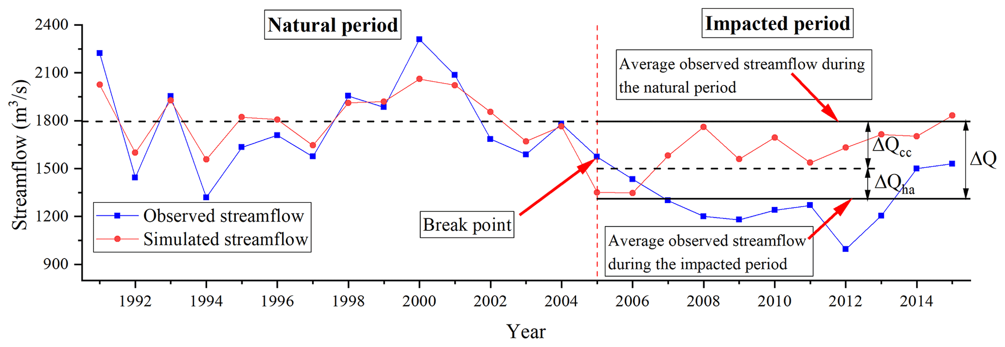
Figure 3 Schematic diagram of the contribution rate (CR) of climate change (CC) and human activities (HAs) to streamflow change using SWAT modeling. (Notation: ΔQ, ΔQ_cc, and ΔQ_ha, respectively, represent the amount of streamflow change in the impacted period, the amount of streamflow change caused by CC, and the amount of streamflow change caused by human activities.)

The hydrological and meteorological data in the natural period are input into the SWAT model, and using the SUFI-2 method to calibrate the model, a set of parameters represents the characteristics of the catchment under natural conditions with less impact from HAs. Then, this set of parameters is brought back into the SWAT model using the meteorological data of the impacted period. Based on the above simulation results, the CC induced in streamflow can be calculated as follows:

$$\begin{array}{}\text{(12)}& \mathrm{\Delta }{Q}_{\mathrm{cc}}={\stackrel{\mathrm{‾}}{Q}}_{\mathrm{si}}-{\stackrel{\mathrm{‾}}{Q}}_{\mathrm{sn}},\end{array}$$

where ${\stackrel{\mathrm{‾}}{Q}}_{\mathrm{si}}$ and ${\stackrel{\mathrm{‾}}{Q}}_{\mathrm{sn}}$ represent the mean simulated annual streamflow (m³ s⁻¹) for the impacted period and natural period, respectively. Thus, the streamflow change induced by HAs can be calculated by the following equation:

$$\begin{array}{}\text{(13)}& \mathrm{\Delta }{Q}_{\mathrm{ha}}=\mathrm{\Delta }Q-\mathrm{\Delta }{Q}_{\mathrm{cc}}.\end{array}$$

After the calculation of ΔQ_cc and ΔQ_ha, the CRs of CC and HAs to streamflow changes, which are defined as CR_cc and CR_ha, respectively, can be estimated as

$$\begin{array}{}\text{(14)}& {\displaystyle }{\mathrm{CR}}_{\mathrm{cc}}={\displaystyle \frac{\left|\mathrm{\Delta }{Q}_{\mathrm{cc}}\right|}{\left|\mathrm{\Delta }Q\right|}}\times \mathrm{100}\mathit{\%},\text{(15)}& {\displaystyle }{\mathrm{CR}}_{\mathrm{ha}}={\displaystyle \frac{\left|\mathrm{\Delta }{Q}_{\mathrm{ha}}\right|}{\left|\mathrm{\Delta }Q\right|}}\times \mathrm{100}\mathit{\%}.\end{array}$$

Equations (12) to (15) are also applicable to quantify the CR of CC and HAs to streamflow changes on a monthly scale.

3.4.2 Construction of the PHD of the CR of CC and HAs

Before the construction of the PHD of the CR of CC and HAs, the sensitivity of the parameters of the SWAT model is first conducted. Based on the related published literature (Zhao et al., 2018a; Yang et al., 2008; Malagò et al., 2015) and the authors' experience, the Latin hypercube and global sensitivity methods were used to perform the uncertainty analysis (Abbaspour et al., 2007). The global sensitivity analysis method is the estimation of the average change in the objective function caused by the change in each parameter, and all parameters change during the whole process. A t test was used to identify the relative sensitivity of each parameter. Considering the influence of the snowmelt streamflow process upstream of the LR basin on the hydrological simulation, 22 parameters were selected, and the details of these selected parameters are shown in Table 2. According to the suggestion of Abbaspour et al. (2004), 500 simulations were set up to implement the sensitivity analysis. The t stat and P values were used to measure which parameters were more sensitive, where a larger absolute t-stat value and a smaller absolute P value represent a higher sensitivity of a given parameter.

Table 2 Twenty-two selected SWAT model parameters in the sensitivity analysis at Yunjinghong station.

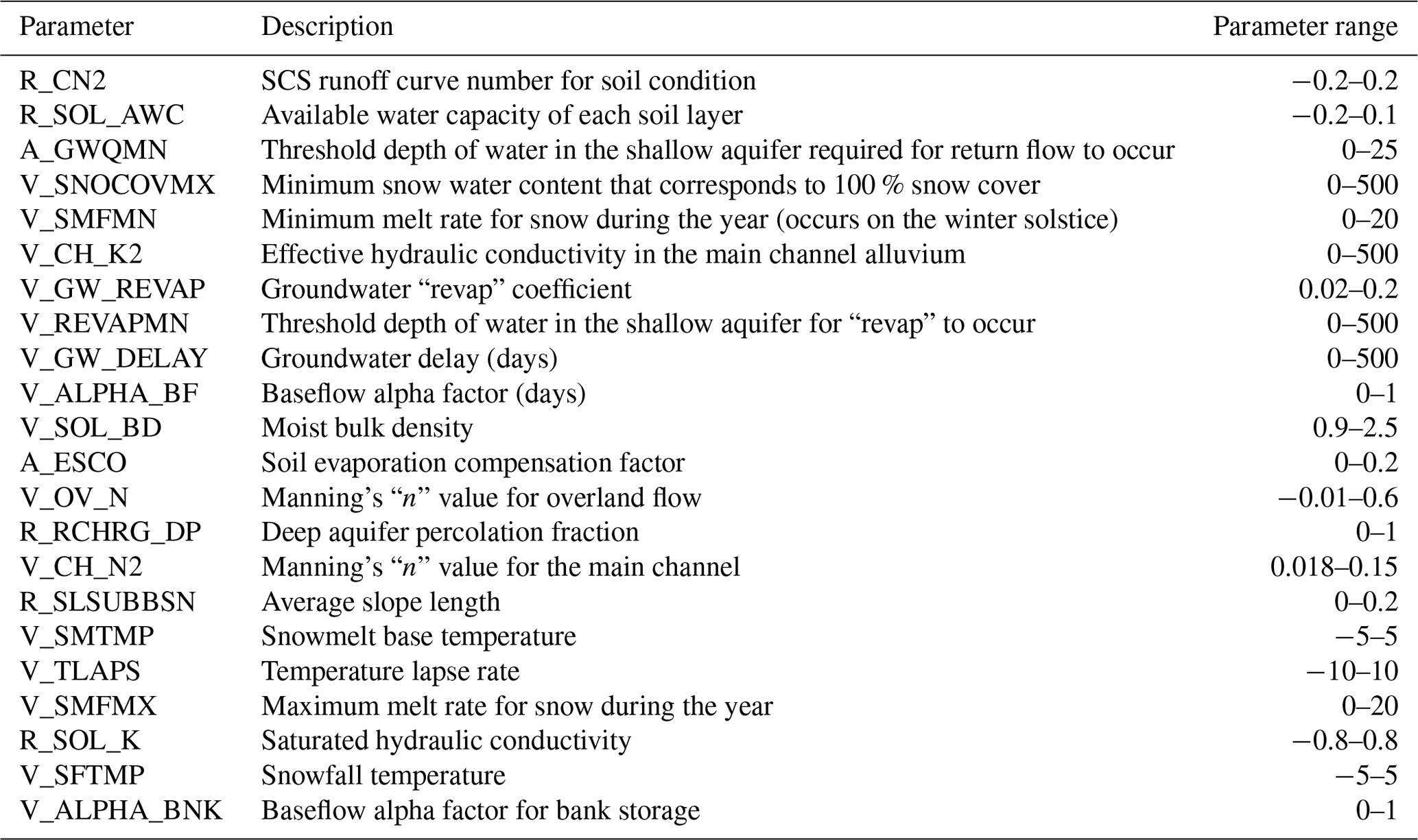
(Notation: R_, V_, and A_represent multiplying, replacing, and adding the corresponding parameter values, respectively, in the process of calibrating the parameters.)

Based on the sensitivity analysis results, nine parameters with the highest sensitivity were selected to recalibrate the model with 1000 simulations. According to the recommendations in Tuo et al. (2016) and Moriasi et al. (2007), the performance of the hydrological simulation can be divided into four grades based on the NSE values: very good performance (0.75 ≤ NSE < 1), good performance (0.65 ≤ NSE < 0.75), satisfactory performance (0.5 ≤ NSE < 0.65), and unsatisfactory performance (NSE < 0.5). According to this evaluation standard, we selected simulation results with NSE greater than 0.75 out of 1000 simulation results to construct the posterior histogram frequency distribution (PHD) of the CR of CC and HAs to streamflow changes using the method introduced in Sect. 3.4.1. Note that to reduce the random error caused by the number of samples, we set the number of simulations with NSEs ≥ 0.75 to be more than 500; that is, we needed to repeatedly use Latin hypercube sampling and the SUFI-2 algorithm until the number of simulation results that met the conditions was more than 500. Then, the CR of more than 500 groups of CC and HAs to streamflow change was calculated. Finally, the PHD of the CR of CC and HAs was constructed in 5 % steps. At this stage, the histogram column with the highest frequency in the PHD was selected as the result of quantitative analysis, which considered the uncertainty, and the arithmetic average of all results in the column was used as the actual value of the CR of CC and HAs.

3.5 Comparison of the newly developed quantification method with the other two methods

In order to evaluate the calculation accuracy of the novel framework proposed in this study to quantify the CR of CC and HAs to streamflow changes, the Budyko framework was used first. This framework was developed by Budyko (1961) and links climate variability to streamflow (Q) and actual evapotranspiration (AE) through the assumption that the long-term average annual catchment AE is determined by the catchment average precipitation (P) and the catchment potential evapotranspiration (PET) (Liu and Liang, 2015). Over the past few decades, the Budyko framework and its variants have been widely used to conduct CC and HA attribution analyses of streamflow changes (Liu et al., 2017; Han et al., 2019; Xin et al., 2019). According to its theoretical assumptions, the multiyear average water balance within the catchment can be expressed as follows:

$$\begin{array}{}\text{(16)}& \mathrm{\Delta }S=P-\mathrm{AE}-Q,\end{array}$$

where P, Q, and AE represent the multiyear average precipitation (mm), streamflow (mm), and actual evapotranspiration (mm), respectively. ΔS (mm) is the change in the amount of water storage at the watershed scale, and it is reasonable to assume that it is equal to 0 on the multiyear average scale. According to Zhang et al. (2001), the AE can be calculated by the following formula:

$$\begin{array}{}\text{(17)}& {\displaystyle \frac{\mathrm{AE}}{P}}={\displaystyle \frac{\mathrm{1}+\mathit{\omega }\left(\mathrm{PET}/P\right)}{\mathrm{1}+\mathit{\omega }\left(\mathrm{PET}/P\right)+{\left(\mathrm{PET}/P\right)}^{-\mathrm{1}}}},\end{array}$$

where ω is the plant-available water coefficient which is related to the vegetation type of the catchment. According to the method for selecting the value of ω provided in Zhang's research (Zhang et al., 2001) and based on the multiyear average AE / P (0.55) and PET $/$ P (0.96) values in the LR basin, this study set the value of ω to 0.5.

The changes in the catchment streamflow due to CC, which are mainly characterized by precipitation (P) and actual evapotranspiration (AE), can be expressed as follows:

$$\begin{array}{}\text{(18)}& \mathrm{\Delta }{Q}_{\mathrm{cc}}=\mathit{\alpha }\mathrm{\Delta }P+\mathit{\beta }\mathrm{\Delta }\mathrm{AE},\end{array}$$

where ΔQ_cc (mm) represents the streamflow changes induced by CC, α and β represent the sensitivity of streamflow to precipitation and actual evapotranspiration, respectively, and ΔP and ΔAE are the changes in precipitation and actual evapotranspiration in the impacted period compared with the natural period, respectively. The sensitivity coefficients α and β are defined as follows:

$$\begin{array}{}\text{(19)}& {\displaystyle }\mathit{\alpha }={\displaystyle \frac{\mathrm{1}+\mathrm{2}\mathrm{DI}+\mathrm{3}\mathit{\omega }\mathrm{DI}}{{\left(\mathrm{1}+\mathrm{DI}+\mathit{\omega }{\left(\mathrm{DI}\right)}^{\mathrm{2}}\right)}^{\mathrm{2}}}},\text{(20)}& {\displaystyle }\mathit{\beta }=-{\displaystyle \frac{\mathrm{1}+\mathrm{2}\mathit{\omega }\mathrm{DI}}{{\left(\mathrm{1}+\mathrm{DI}+\mathit{\omega }{\left(\mathrm{DI}\right)}^{\mathrm{2}}\right)}^{\mathrm{2}}}},\end{array}$$

where DI is the dryness index which is equal to $\mathrm{PET}/P$.

Through the above formulas, we can separate the CR of CC to streamflow variations and further compare it with the calculation results of the new method proposed in this paper.

In addition to the Budyko framework, we also used the GMSWU data introduced in Sect. 2.2 and the reservoir dead storage capacity data to roughly separate the CR of HAs from the streamflow changes in the LR basin. The GMSWU data set provides five types of water withdrawals (i.e., irrigation, livestock, domestic use, mining, and manufacturing) within the period of 1970 to 2010 in the LR basin, and it was generated by downscaling country-scale estimates of different sectoral water withdrawals from the Food and Agriculture Organization (FAO) of the United Nations AQUASTAT, which ensured its good accuracy (Huang et al., 2018). Here, AQUASTAT refers to the FAO's Global Information System on Water and Agriculture (http://www.fao.org/aquastat/en/, last access: 16 October 2022). Catchment-scale annual water use data were calculated by spatially averaging all grids within the LR basin, and then streamflow changes caused by each type of water use were obtained using the average annual water use value during the impacted period minus that during the natural period. As shown by Han et al. (2019) and Zhao et al. (2012), during the past 2 decades, dam construction has been the most significant HA affecting the streamflow changes in the LR basin. Therefore, in this study, we converted the dead storage capacity of six large reservoirs (Table 1) into units of millimeters according to their watershed control area because the impact of the reservoir on the outlet flow of the watershed can be used as its minimum impact value on the multiyear average scale. It should be pointed out that here we use two seemingly simpler methods to verify the computational results of the new framework proposed in this study. However, this does not reduce the innovation of this study, as the new framework has the following significant advantages over the other two methods. (1) The new framework can perform quantitative calculations on the annual and monthly scales. (2) It has relatively fewer data requirements. (3) It has a more explicit physical meaning.

4 Results

4.1 Hydrological and meteorological trends in the LR basin

4.1.1 Trends and break points of the streamflow

The results of the Mann–Kendall break point test for the annual streamflow at Yunjinghong station within the period from 1961 to 2015 are shown in Fig. 4. Since the intersection of the UF and UB curves in Fig. 4 is within the confidence intervals (of 0.05 and 0.01), the break point of the annual streamflow in the LR basin occurred in 2005. Combined with the construction of reservoirs in the LR basin, the construction of the Xiaowan hydropower station started in October 2004 (with total storage capacity = 15.3 km³). Therefore, according to the principle of time division introduced in Sect. 3.1, the study period can be divided into the natural period (from 1961 to 2004) and the impacted period (from 2005 to 2015). UF curves of the MK break point test represent the trend of the time series. As shown in Fig. 4, the observed annual streamflow at Yunjinghong station had an increasing trend before 1967, after which the annual streamflow experienced a significant decreasing trend until 2015.

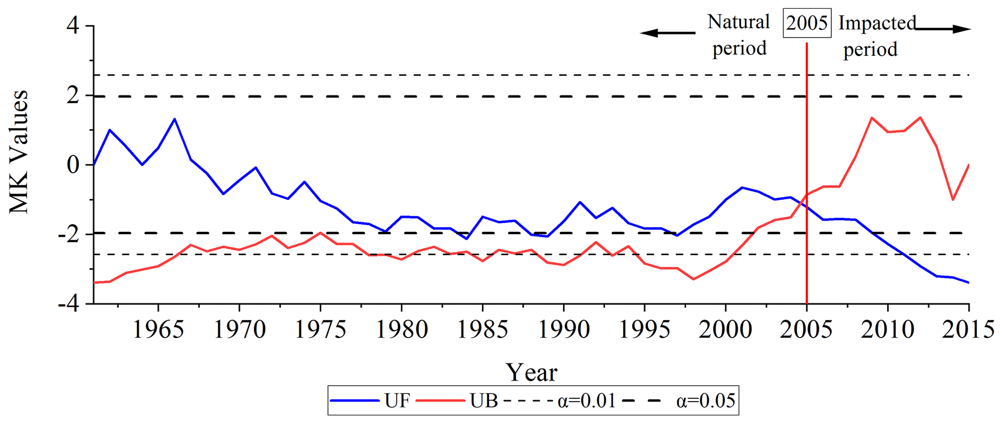
Figure 4 The Mann–Kendall break point testing statistics of the annual streamflow for the LR basin from 1961 to 2015.

Figure 5 shows the MK monotonic trend testing statistics of the annual and monthly streamflow for the LR basin from 1961 to 2015. A positive Z statistic represents an upward trend in the time series, and vice versa. The annual average streamflow in the LR basin showed a significant decreasing trend and passed the 0.01 significance level. This decreasing trend of the annual streamflow in the LR basin is consistent with the conclusions of Han et al. (2019). For the monthly streamflow, the streamflow from February to May showed an increasing trend, among which March and May passed the significance level of 0.05 (with the Z statistic greater than 1.96). The streamflow in the remaining months showed a decreasing trend. Except for June, the decreases in the other months all passed the 0.05 significance level. The decrease in the streamflow from August to October even passed the 0.01 significance test. Among them, the largest decrease was in August (Z statistic = −4.23). This trend of changes in streamflow during the year was mainly caused by the operation of reservoirs within the basin, because reservoirs often release flows during dry periods (from January to May) to alleviate possible droughts in the downstream areas, and they store water during wet periods (from June to October) to reduce the flood control pressure in the downstream area below the reservoir.

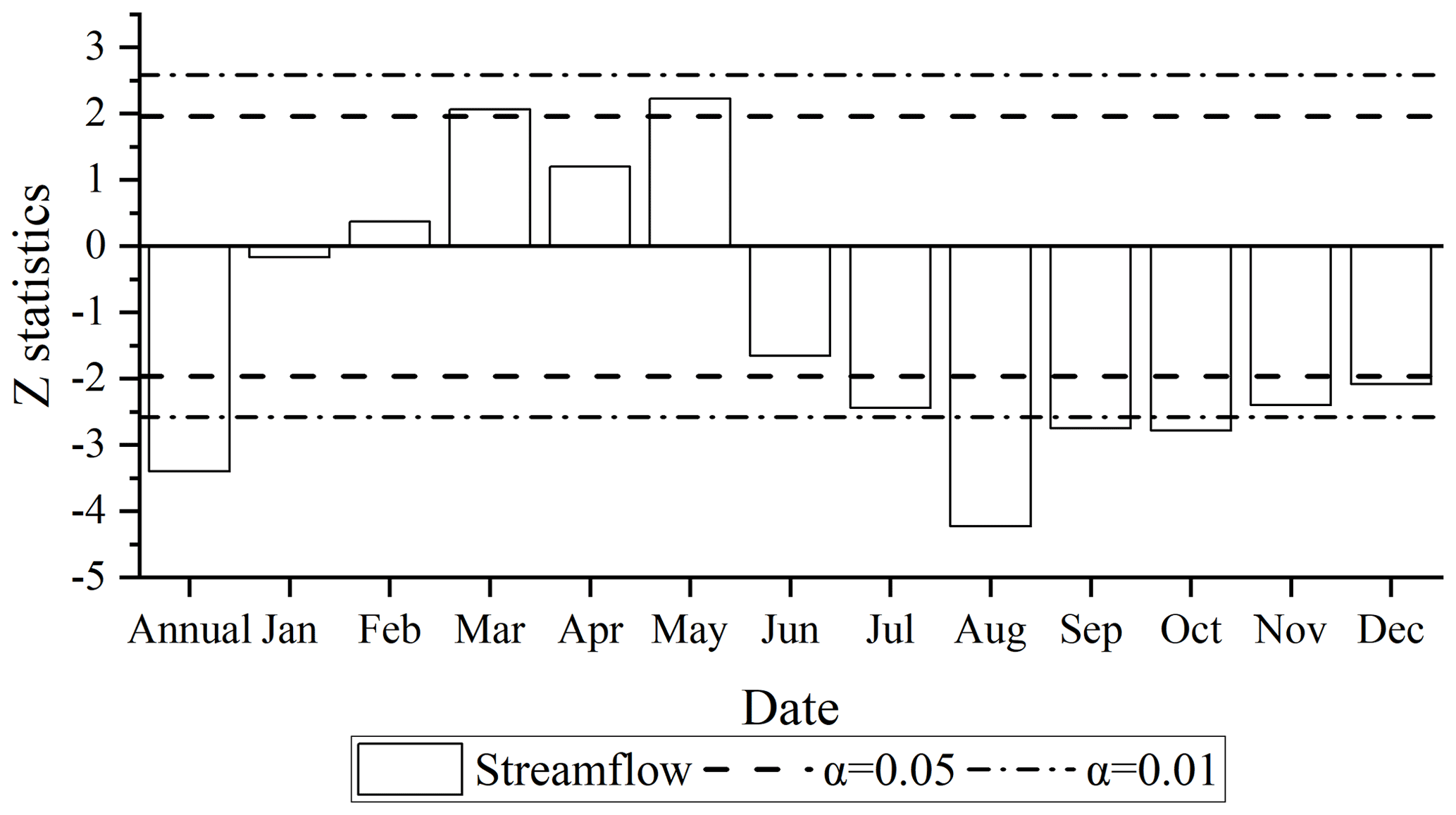
Figure 5 The Mann–Kendall monotonic trend test statistics of the annual and monthly streamflow for the LR basin from 1961 to 2015.

4.1.2 Trends and break points of the mean areal precipitation and temperature

The time series and MK break point test results of the annual areal precipitation and mean temperature for the LR basin from 1961 to 2015 are presented in Fig. 6. In general, changes in the annual precipitation were more complicated than changes in the mean temperature in the LR basin. The precipitation showed a fluctuating trend, while the mean temperature almost showed a continuous rising trend throughout the study period.

Figure 6 Time series and the Mann–Kendall break point test statistics of the annual precipitation (a) and mean temperature (b) in the LR basin from 1961 to 2015.

As shown by the time series of the annual precipitation in the LR basin in Fig. 6a, there was a slightly decreasing trend in the LRB during the last 55 years, especially in the past 10 years, but this trend was not significant according to the result of the MK test at the α= 0.05 significance level. The areal annual precipitation in 1985 reached 971 mm, which was the highest in the last 55 years. In 2009, it was 769 mm, which was the lowest value from 1961 to 2015. The MK break point test results showed that there were 11 break points in the annual precipitation time series. Regarding the positive and negative changes in the UF value, the annual precipitation showed a fluctuating trend from 1961 to 1966; then, until 1998, the annual precipitation showed a small decreasing trend (except in 1991); from 1999 to 2006, the annual precipitation experienced a small increase, and in the last 9 years (2007–2015), the annual precipitation in the study area showed a decreasing trend.

The time series of the annual mean temperature in the LR basin presented in Fig. 6b shows that the annual mean temperature in the study area changed relatively smoothly before 1998. After 1998, the temperature began to rise significantly and exceeded the significance level of 0.01. The annual mean temperature in 1963 reached 5.2^∘, the coldest temperature in the study period. The hottest year was 2009, during which the mean temperature was 7.2^∘. In terms of changes in the UF value, the mean temperature showed a fluctuating trend from 1961 to 1968 and then continued to rise until it exceeded the significance level of 0.05 in 1991 and exceeded the significance level of 0.01 in 1998. The break point of the annual mean temperature was detected in 1997.

The MK monotonic trend test statistics of the annual and monthly precipitation and mean temperature for the LR basin from 1961 to 2015 are presented in Fig. 7. The annual precipitation in the study area showed an insignificant decreasing trend (Z statistic = −0.55), while the annual average temperature showed a significant increasing trend (Z statistic = 6.02) and exceeded the significance level of 0.01. The monthly change in precipitation also showed a fluctuating trend. The increasing trend of precipitation in April and the decreasing trend of precipitation in June exceeded the significance level of 0.05, while the trends of precipitation in the other months were not significant (|z statistic| < 1.96). The trend of the monthly mean temperature was relatively simple. Except for the increase in the mean temperature in November, which passed the significance level of 0.05, the increasing trend of the mean temperature in all the other months passed the significance level test of 0.01. This also means that the climate in the study area has been gradually warming and drying during the past 55 years.

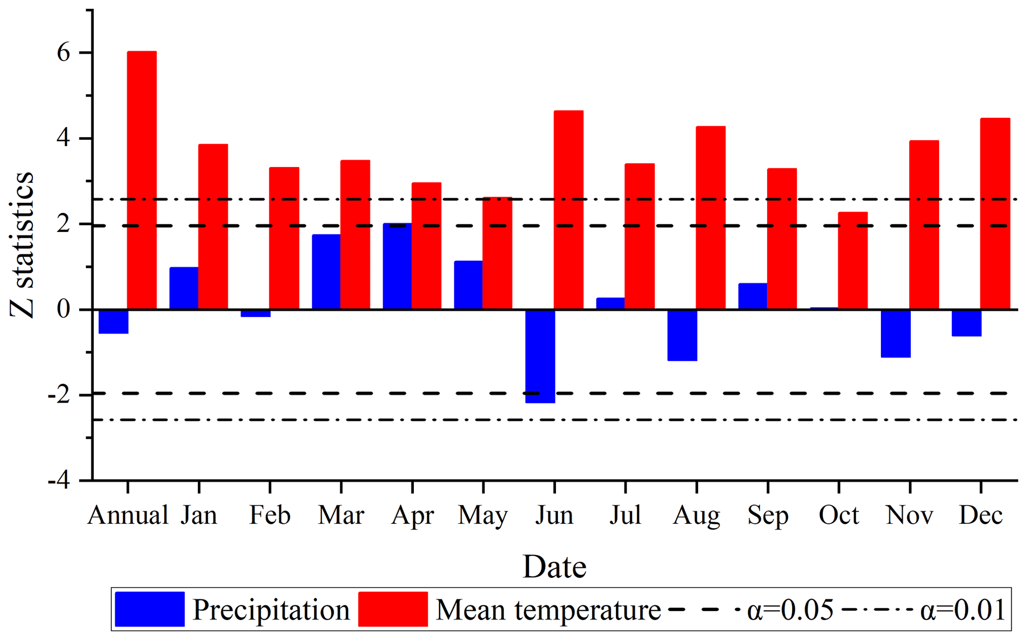
Figure 7 The Mann–Kendall monotonic trend test statistics of the annual and monthly precipitation and mean temperature for the LR basin from 1961 to 2015.

4.2 Results of the SWAT simulations

4.2.1 Sensitivity analysis of the SWAT model parameters

As described in Sect. 3.4.2, the sensitivity of 22 selected parameters was evaluated using the SWAT-CUP software (Abbaspour et al., 2007; Abbaspour et al., 1997), and this software integrates the global sensitivity analysis method and the parameter optimization methods (such as SUFI-2). SWAT-CUP can perform a combined optimization and uncertainty analysis using a global search procedure and deal with a large number of parameters through Latin hypercube sampling. The sensitivity evaluation indexes, the t stat and P value, of 22 parameters are shown in Table 3. Obviously, the sensitivity ranks of the parameters calculated based on SUFI-2 showed that ALPHA_BNK has the highest sensitivity, followed by CH_K2, SOL_BD, GW_REVAP, SFTMP, CN2, SOL_K, SMTMP, and ALPHA_BF, whereas the other 14 parameters have less sensitivity for the streamflow simulation. ALPHA_BNK mainly controls the baseflow process within the watershed, and this parameter has also proven to have high sensitivity in other relevant studies (Wu and Chen, 2015), especially in mountainous areas. CH_K2 and ALPHA_BF are mainly related to groundwater runoff, CN2 is the SCS runoff curve number, and these parameters all have higher sensitivity in many published articles on the SWAT model parameter sensitivity (Zhao et al., 2018a; Wu and Chen, 2015). Other parameters with high sensitivity, such as SFTMP and SMTMP, which mainly control the snowmelt process in the basin, also indicate that snowmelt runoff plays an important role in the recharge of the LR basin (Gao et al., 2019). Based on the above sensitivity analysis results, the top nine parameters of the sensitivity ranking were selected for further research.

Table 3 Basin-wide sensitivity ranking calculated from 22 selected parameters using SUFI-2.

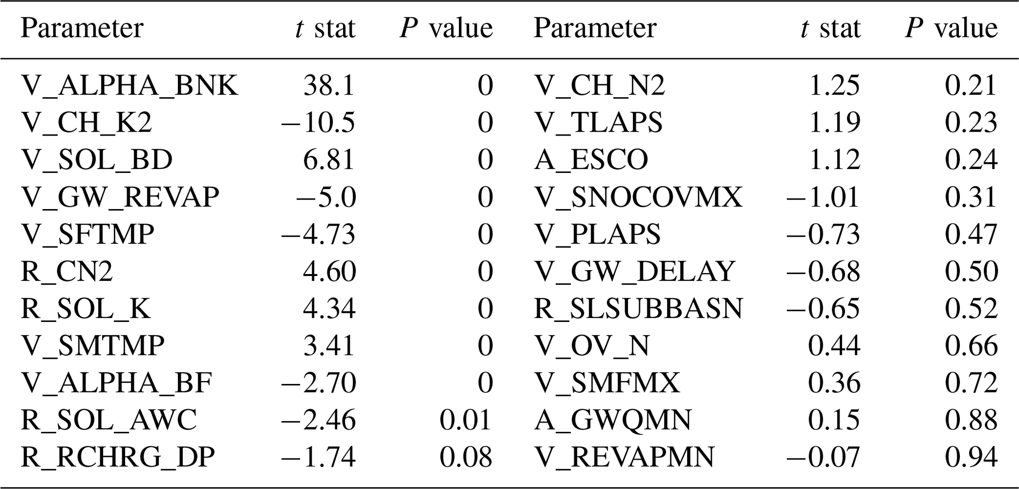
(Notation: V_ represents replacing the default value with the given value, R_ represents the relative change (%), and A_ represents adding the given value to the original parameter value.)

4.2.2 Results of the SWAT simulations

As mentioned above, the nine parameters with the highest sensitivity rankings that controlled different stages of the basin's streamflow production and flow concentration were selected to recalibrate the model using the SUFI-2 method, and the number of simulations was set to 2000. To reduce the influence of the initial value of the model parameters on the simulation results, during the model parameter calibration process, 1961 and 1962 were set as the warming-up period. Table 4 shows the evaluation metrics of the simulation using the SWAT model at a monthly scale with the largest NS value. For the calibration period from 1963 to 1990, the NSE and RE were found to be equal to 0.94 % and −10.62 %, respectively; for the validation period from 1991 to 2004, the model performance was slightly better than that in the calibration period, and the NSE and RE were 0.95 % and −8.65 %, respectively. For the whole period from 1963 to 2004, the NSE (0.94) and RE (−9.97 %) were also satisfactory. According to the requirements of the Information Center of the Ministry of Water Resources, the data provider, this study standardized the observed and simulated runoff curves of Yunjinghong station. Figure 8 shows the normalized monthly observed and simulated streamflow at Yunjinghong station from 1963 to 2004 and the histogram of the mean monthly precipitation in the LR basin. As seen from Fig. 8a and b, the SWAT model can simulate the flow processes very well and almost perfectly matches the observed streamflow curve. Note that the simulated streamflow overestimated the floods in individual years (1973, 1985, and 1995 in Fig. 8b), which might be caused by the uncertainty of the precipitation product (Han et al., 2019). In summary, the SWAT model can better simulate the streamflow process at Yunjinghong station on a monthly scale; therefore, this model is considered suitable for the next part of the research.

Table 4 Evaluation metrics, Nash–Sutcliffe efficiency, and relative error of the SWAT model on a monthly scale.

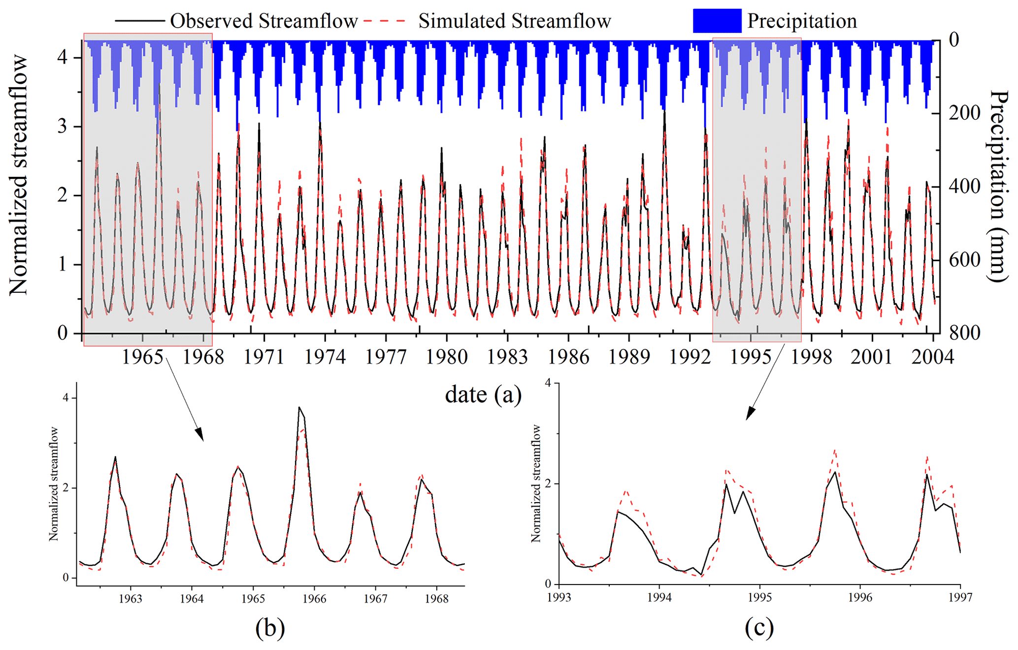
Figure 8 Normalized monthly observed and simulated streamflow at Yunjinghong station for the calibration (from 1963 to 1990) and validation (from 1991 to 2004) periods. The blue histogram shows the monthly precipitation in the LR basin. The normalized streamflow was calculated from the observed and simulated streamflow divided by their average values.

According to the method described in Sect. 3.4.2, simulations with NSEs greater than 0.75 among the 1000 simulations were selected. Figure 9 shows the number of simulations with 0.75 ≤ NSE < 0.8, 0.8 ≤ NSE < 0.85, 0.85 ≤ NSE < 0.9, and 0.9 ≤ NSE < 0.95 during the calibration period (1963–1990), the validation period (1991–2004) and the whole period (1963–2004) on a monthly scale. In summary, there were 575 simulations with NSEs greater than 0.75 out of 1000 simulation results during the calibration period, the validation period, and the whole period. Clearly, the NSEs of most simulation results were between 0.75 and 0.9, with 533, 537, and 533 simulations in the calibration period, the validation period, and the whole period, respectively, and only a few simulation results had NSEs greater than 0.9. In the different periods, the model performed well in the validation period compared with that in the calibration period, which indicated that the model has good predictive ability in the LR basin.

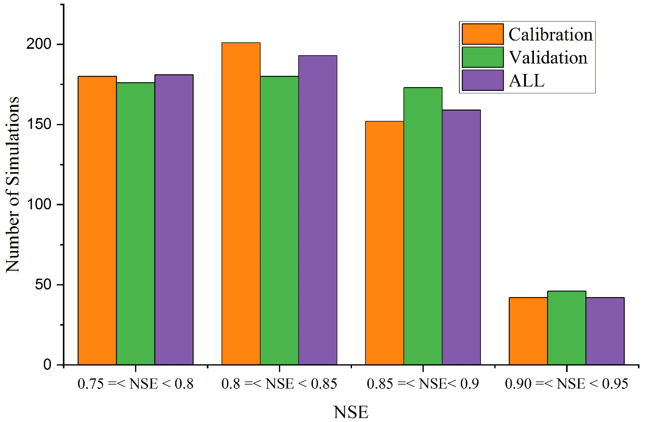
Figure 9 Number of simulations with NSEs greater than 0.75 during the calibration (1963–1990), validation (1991–2004), and whole periods (1963–2004).

4.3 Quantification of CC and HAs for streamflow change considering the uncertainties

4.3.1 Quantification of the impacts considering the uncertainties at the annual scale

The 575 simulations with NSEs greater than 0.75 were selected to construct the posterior histogram frequency distribution (PHD) of the CR of CC and HAs to streamflow changes in the LR basin. Figure 10 shows the number of simulations of the CC CR in 5 % intervals and their corresponding NS box plots. In total, 167 out of 575 simulations calculated that the CR of CC in the LR basin to runoff reduction was 40 %–45 %, and the average NSE was 0.84. Then, 131 and 92 of the simulation results had calculated climate CRs of 35 %–40 % and 45 %–50 %, respectively. The CR of CC in other intervals had relatively few simulations. The NSE value of the CR between 70 % and 75 % was largest (NSE = 0.86), but it had only one simulation. Therefore, when using hydrological simulations to quantify the CR of CC and HAs to the streamflow change in the watershed, not only the merits of the model performance, but also the uncertainty of the model simulation should be considered. In general, according to the results calculated by the new quantitative framework proposed in this paper, streamflow changes in the LR basin duo to CC accounted for 40 %–45 % (with an average CR of 42.6 %), and the corresponding HAs accounted for 55 %–60 % (with an average CR of 57.4 %).

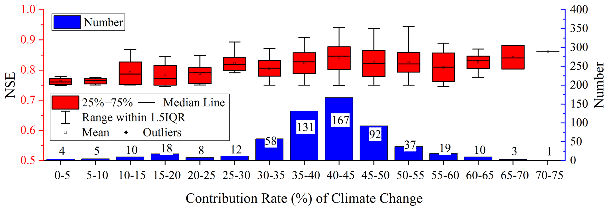
Figure 10 Histogram of the number of simulations of the CR (with 5 % steps) of climate change to streamflow reduction in the LR basin at the annual scale and corresponding Nash–Sutcliffe efficiency box plots.

Table 5 shows the average values of the main hydrological and meteorological elements and their changes during the natural period and the impacted period. During the impacted period, compared with the natural period, the multiyear average streamflow decreased by 396 m³ s⁻¹ (86.5 mm) and the precipitation decreased by 25 mm; as basin-wide temperatures increased, the mean potential evapotranspiration and temperature in the basin increased by 6.4 mm and 0.9 ^∘C. In terms of relative changes, the streamflow decreased by 22 %, but precipitation and potential evapotranspiration changed by −2.9 % and 6.4 %, respectively, which may indicate that the streamflow reduction in the LR basin was mainly caused by HAs.

Table 5 Hydrological and meteorological elements in the natural (1963–2004) and impacted periods (2005–2015) of the LR basin and their changes during the two periods.

4.3.2 Quantification of the impacts considering the uncertainties on a monthly scale

The monthly CR of CC and HAs to the changing streamflow at Yunjinghong station was also analyzed using the new framework proposed in this study, and the results are shown in Fig. 11. In general, only June and November had a large CR of CC, which reached 95 %–99.9 % and 70 %–75 %, respectively, while the CR of CC in the other 10 months was relatively small. The trends of the streamflow and the precipitation and mean temperature in the study area shown in Figs. 5 and 7 indicate that the streamflow in June and November showed a decreasing trend (Fig. 5), while the precipitation in June decreased significantly (passing the significance level of 0.05), and the temperature increased significantly (passing the significance level of 0.05) (Fig. 7). This significant decrease in precipitation and the significant increase in temperature were the main reasons for the decrease in the streamflow in June; that is, the decrease in the streamflow in June was mainly caused by CC. The main factors that led to the decrease in the streamflow in November were also the decrease in precipitation and the significant increase in temperature (Fig. 7). From the results of each month, the CR of CC in March and April was the smallest, reaching 10 %–15 %, followed by July (15 %–20 %), May, August, and September (20 %–25 %), October (25 %–30 %), January and February (30 %–35 %), and December (45 %–50 %).

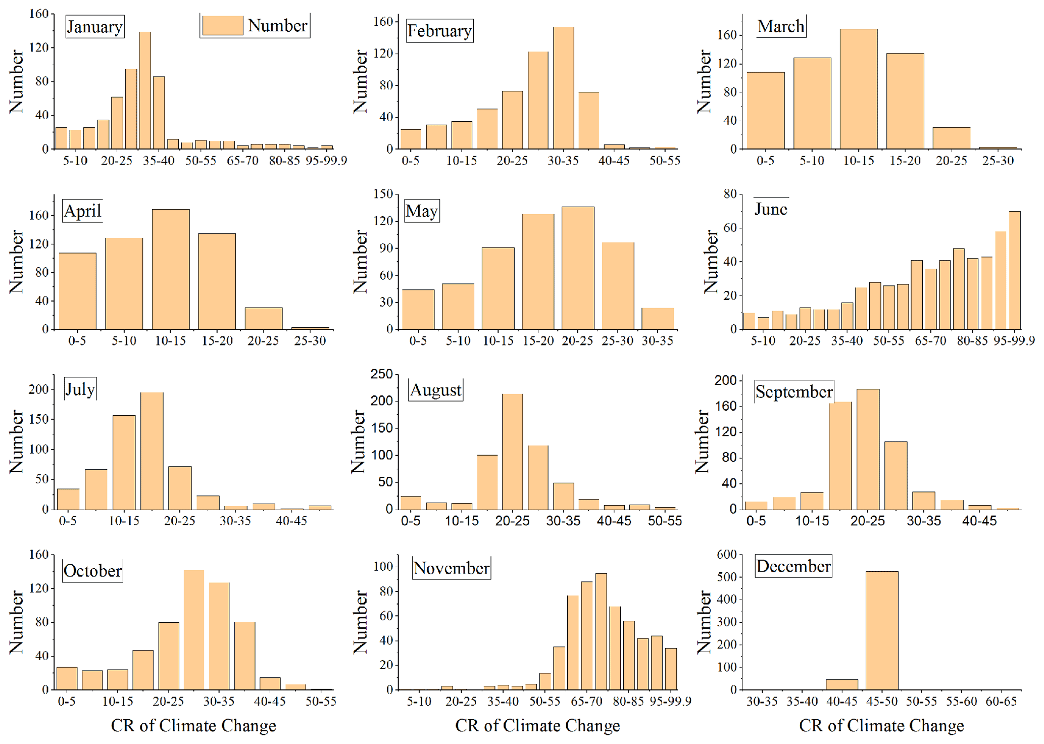
Figure 11 Histogram of the number of simulations of the CR (with a 5 % step) of climate change to streamflow reduction in the LR basin on a monthly scale.

The mean CR of CC and HAs at the monthly scale, which was calculated by averaging the CRs of all simulation results within the highest frequency, is displayed in Fig. 12a, and the monthly precipitation, potential evapotranspiration, and runoff depth during the natural period and the impacted period are shown in Fig. 12b. Overall, the monthly CR was consistent with the annual results, and the CR in a total of 10 months was mainly due to HAs that led to a decrease in the streamflow in the LR basin. It is worth noting that the CR of CC in June reached 96 %. Figure 12b shows that the precipitation in June during the impacted period was significantly reduced compared with the natural period (with a 20.2 mm decrease). At the same time, the increase in potential evapotranspiration in June was also relatively obvious (with a 9.2 mm increase). Figure 12b clearly shows that the streamflow in the LR basin during the impacted period was significantly reduced compared with the natural period in June to October, and the precipitation had little change, except in June. Therefore, we can conclude that the main reason for the decrease in the streamflow in the LR basin was HAs, as shown in Fig. 12a. In this study area, the main cause of the streamflow changes was mainly due to the construction of reservoirs (such as Manwan and Xiaowan), and at the same time, the water storage of these water conservancy facilities during the flood period also provided engineering support for protecting the safety of downstream life and property. Conversely, during the dry season (from January to May), the streamflow in the impacted period showed an increasing trend compared with the natural period, and the increase in runoff during these 5 months was mainly due to HAs (Fig. 12a), which might have been caused by the release of water from the reservoirs during the dry season. For example, in 2016, due to the influence of El Niño, the countries along the lower Mekong River all suffered severe drought. The Chinese government immediately asked the Jinghong Reservoir to release water urgently, which effectively helped downstream countries mitigate a series of possible effects caused by drought and water shortages (D. Li et al., 2017).

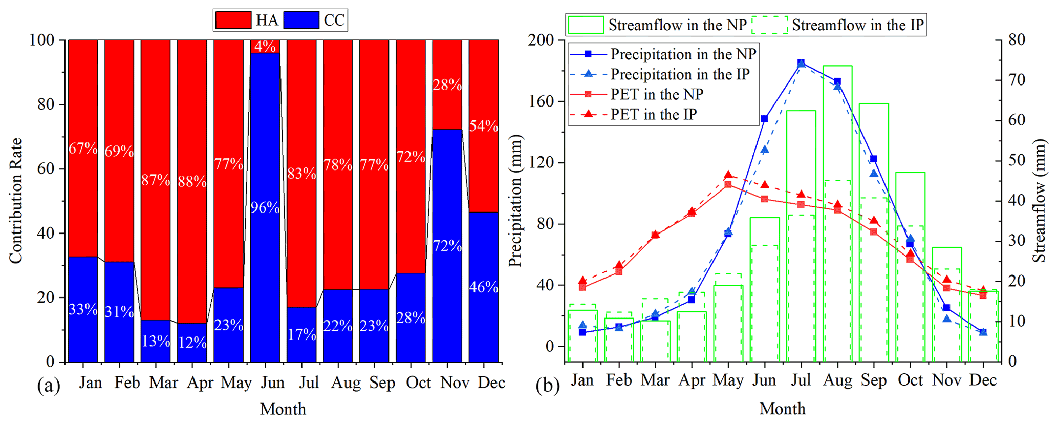
Figure 12 CR of CC and human activities to the changing monthly streamflow at Yunjinghong station (a), monthly precipitation, potential evapotranspiration, and runoff depth during the natural period and the impacted period in the LR basin (b). (Notation: HA: “human activities”, CC: “climate change”, PET: “potential evapotranspiration”, NP: “natural period”, and IP: “impacted period”.)

4.4 Comparison with the other two methods

In this subsection, the new proposed framework that considers the uncertainty of hydrological simulations was compared with the Budyko framework, five sections of water withdrawal data from the LR basin, and the equivalent streamflow depth converted from the dead storage capacity of six large hydropower stations.

Table 6 shows the CR of CC and HAs to annual streamflow changes at Yunjinghong station, which was calculated from the Budyko framework. The actual evapotranspiration was calculated from the annual precipitation minus the annual streamflow depth. As shown in Table 6, compared with the natural period, the precipitation and streamflow depth in the impacted period showed a decreasing trend.

Table 6 CR of climate change (CC) and human activities (HAs) calculated by the Budyko framework.

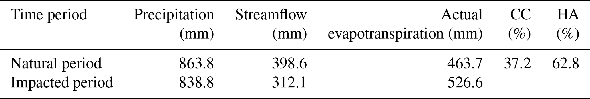
The precipitation decreased by 25 mm, and the streamflow depth decreased by 86.5 mm. In contrast, the actual evapotranspiration showed an increasing trend, which may be related to the continuous increase in temperature in recent decades. The CR of CC and HAs to streamflow changes accounted for 37.2 % and 62.8 %, respectively, which was basically consistent with the results calculated by the new framework proposed in this study (the difference was 5.4 %).

Figure 13 shows the annual water withdrawals (i.e., domestic, irrigation, livestock, manufacturing, and mining) in the LR basin during the period from 1970 to 2010 and changes in the installed capacity and dead reservoir storage from 1992 to 2015. In addition to the amount of water use for irrigation, the other four types of water use withdrawals all showed an increasing trend from 1970 to 2010, with domestic water consumption increasing the most (linear slope = 0.043). The comparison between the impacted period and the natural period showed that the other four types of water consumption, except for domestic water use, all had a larger increase in the natural period than during the impacted period. To meet the power generation needs of Southwest China and the flood control and drought resistance requirements of downstream countries, the total dead storage capacity and total installed capacity of the reservoirs from 1992 to 2015 all showed a significant increase, especially after the construction of Nuozhadu hydropower station in 2012, shown in Fig. 1.

Figure 13 Annual water withdrawals of the LR basin during the period from 1970 to 2010. The linear trend lines are indicated by blue (1970–2004), green (2005–2010), and red (1970–2010), and in the last panel, the total dead storage capacity and installed capacity of the LR from 1992 to 2012 are shown.

According to the method introduced in Sect. 3.5, the changes in the streamflow caused by HAs in the LR basin were separated, which mainly included the five sections of water consumption changes and the same amount of water depth as the total dead storage capacity of the reservoir. Figure 14 shows the CR of the five types of water withdrawals by HAs and the construction of the reservoirs to the streamflow changes in the LR basin during the impacted period (from 2005 to 2015) compared with the natural period (from 1961 to 2004). Overall, the CR of HAs to streamflow changes was 59.91 %, while that of CC was 40.09 %. This result was also consistent with the results calculated in Sect. 4.3.1. Among them, the streamflow depth caused by the construction of the reservoir was reduced by −50.17 mm, which was also the factor that had the greatest impact on streamflow compared with other HAs, and its CR reached 58.0 %, while the CR of the other five types of water withdrawal was relatively small. The CRs of domestic, irrigation, livestock, manufacturing, and mining water withdrawals were 1.32 %, −0.35 %, 0.12 %, 0.79 %, and 0.03 %, respectively, a total of 1.91 %. In other words, the decrease in the streamflow in the LR basin was mainly due to the impact of HAs, and most of it was caused by the construction of the reservoirs.

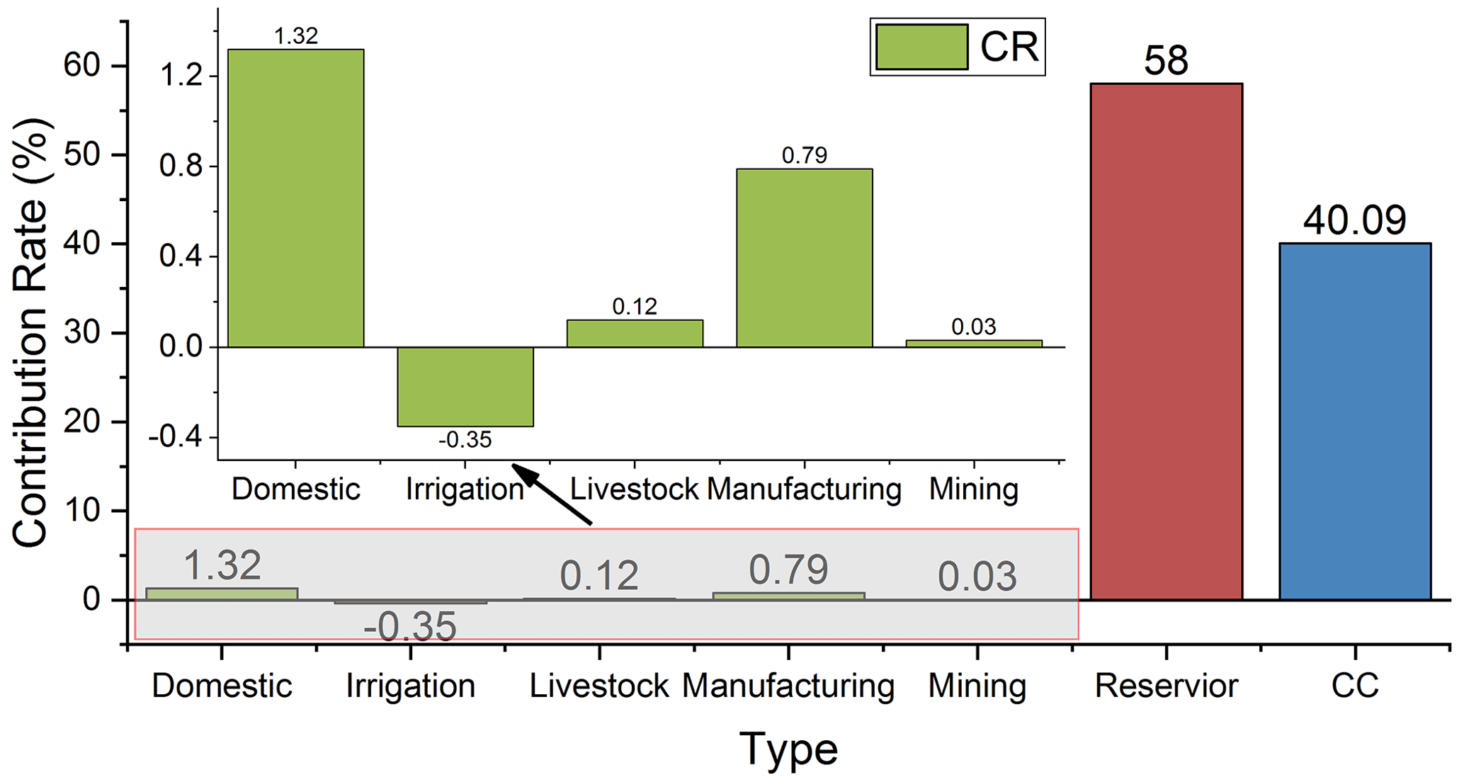
Figure 14 CR of domestic, irrigation, livestock, manufacturing, and mining water withdrawals and reservoir construction and CC to the streamflow changes at Yunjinghong station from 1961 to 2015.

5 Discussion

5.1 How does parameter uncertainty affect the quantitative results?

In this paper, we proposed a novel framework to quantify the CR of CC and HAs to streamflow changes considering the uncertainty of hydrological simulations. This is because the phenomenon of “equifinality for different parameters” in hydrological simulations greatly affects the quantification results. To preliminarily investigate the impact of model simulation uncertainty of the quantitative results, we selected the two simulation results with the largest NSEs in this study for analysis. The evaluation metrics and CR of CC and HAs are shown in Table 7, which shows that both simulations can simulate the monthly streamflow at Yunjinghong station in the LR basin accurately, and the two simulations have almost the same evaluation performance. However, the attribution analysis obtained from the two hydrological simulations showed completely different results. In the first simulation result, according to the method introduced in Sect. 3.4.1, the streamflow changes in the LR basin were mainly caused by CC, but in the second hydrological simulation, the opposite conclusion was drawn; that is, HAs dominated. These were almost the same hydrological simulation results but with opposite conclusions from the attribution analysis; this was one of the reasons why we must consider the uncertainty of the model parameters in the attribution analysis of CC and HAs using hydrological simulations. The results of Sect. 4.3.1 and related published studies (Han et al., 2019) in the LR basin show that the streamflow changes in the LR basin were mainly caused by HAs.

Table 7 Results of the CR of climate change and human activities for runoff changes with almost equal model performance (monthly) using the SWAT model.

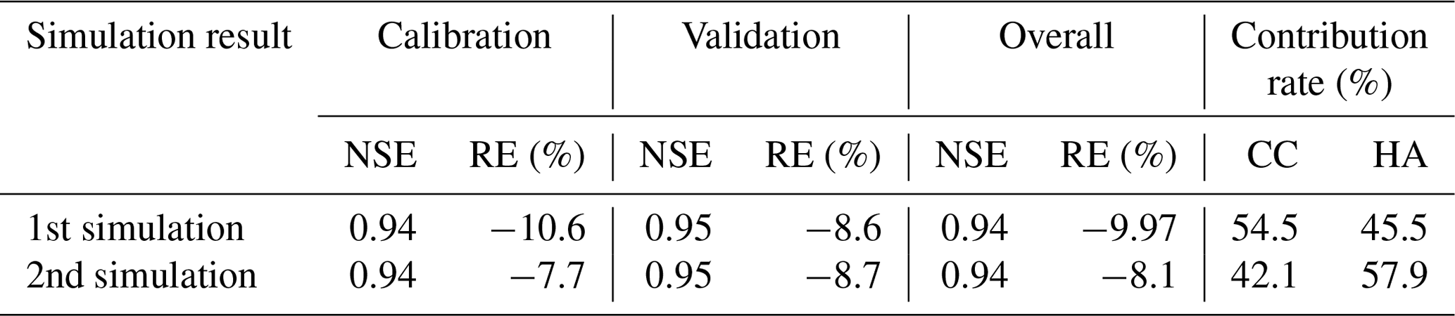
(Notation: CC and HA represent the climate change and human activities, respectively; NSE and RE represent the Nash–Sutcliffe efficiency coefficient and the relative error, respectively.)

Table 8 shows the values of nine highly sensitive parameters of the two simulation results and the streamflow values simulated by the two simulations in the natural period and the impacted period. Table 8 and the calculation methods introduced in Sect. 3.4.1 show that the watershed streamflow reduction caused by CC calculated by the first and second simulation results was −217.1 and −170.6 m³ s⁻¹, respectively, which was the reason why they had opposing calculated attribution results. From the perspective of specific parameter values, the most sensitive parameter is ALPHA_BNK, which was the base flow alpha factor for bank storage (days) characterized by the bank storage recession curve. The difference between the two calibration results was not large, and this parameter was mainly controlled by the baseflow process, having little effect on the average annual streamflow, while the difference in CH_K2 in the two calibration results was larger, at 303.87 and 106.12. This parameter represented the effective hydraulic conductivity of the main channel alluvial layer, which meant that the larger the CH_K2 value is, the more likely the water in the main channel is lost to groundwater; accordingly, the streamflow production at the outlet of the watershed would decrease (Arnold et al., 2012b; Xu et al., 2016; Zhao et al., 2018a). This might also be one of the reasons why the first simulated streamflow (1617 m³ s⁻¹) was slightly smaller than the second one (1667.9 m³ s⁻¹). The SFTMP parameter, which was the temperature when precipitation was converted into snowfall, returned values for the first simulation and the second simulation as 2.69 and −0.11 ^∘C, respectively; this meant that, in the first simulation, more liquid precipitation was converted into a solid state and less streamflow was formed, which also led to a smaller simulated streamflow in the first simulation. The SMTMP parameter, which was the snowmelt base temperature, was −4.13 ^∘C in the first simulation result and 3.73 ^∘C in the second simulation result. From basic physical knowledge, the SMTMP parameter in the second calibration result was more reasonable. Compared with other research results with similar terrain features in this study area, Debele et al. (2010) constructed the SWAT model in the high-altitude area of the source of the Yellow River, China, and the SMTMP value obtained was 4 ^∘C. The difference between the two simulations was not large for the set of the other parameters (SOL_BD, GW_REVAP, CN2, and SOL_K) or the parameter that controlled the baseflow (ALPHA_BF), with little effect on the average streamflow of the basin. Based on the above, the second simulation results were consistent with the calculation results of the new framework proposed in this study. Therefore, when we choose a hydrological simulation to analyze the attribution of CC and HAs to streamflow variations, we should clearly also consider the actual physical meaning and the uncertainties of the model parameters.

Table 8 Values of nine sensitivity parameters with similar simulation results and their simulated streamflow in the natural and impacted periods.

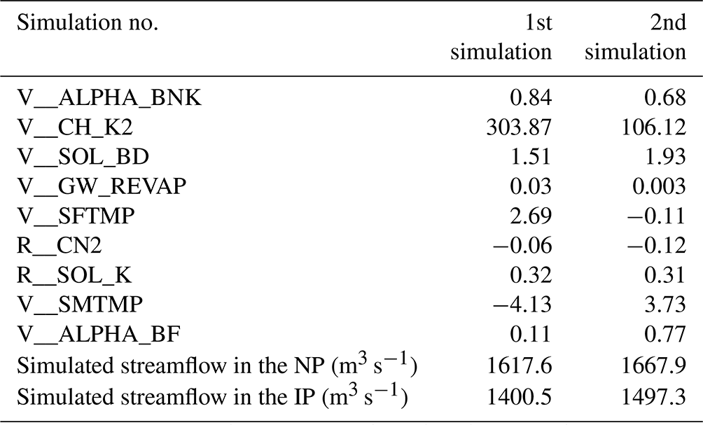
(Notation: NP: “natural period”, IP = : “impacted period”, and R_, V_, and A_represent multiplying, replacing, and adding the corresponding parameter values, respectively, in the process of calibrating the parameters.)

In this study, 575 parameter combinations with good simulation results (NSE greater than 0.75) were selected, with a step size of 5 %: it is proposed to reduce the influence of hydrological modeling uncertainty in the quantitative results by constructing the posterior histogram distribution of the CR of CC and HAs to watershed streamflow change. However, it is undeniable that there are still unreasonable parameter combinations in the simulation results with high probability (167 times). For the LR basin, it is almost impossible to obtain the measured values of all nine parameters with high sensitivity (Table 3). Therefore, in order to further explore the possible influence of unreasonable parameter values on the quantitative results, we selected two parameters related to snowmelt streamflow (SMTMP and SFTMP) to exclude unreasonable parameter combinations. According to the parameter value ranges recommended by Abbaspour et al. (2007) and other related references (Arnold et al., 2012a; Yang et al., 2017), in this study, the reasonable value range of these two parameters is set to −5 to 5^∘. After excluding parameter combinations outside this value range, we obtained 55 simulation results with relatively reasonable parameter values, and the quantization results obtained from this calculation are shown in Fig. 15. It can be seen from Fig. 15 that, after excluding unreasonable parameter combinations, the calculated CR of CC in the LR basin to the reduction of streamflow is 45 %–50 % (with an average CR of 47.1 %), and this result is consistent with the results presented in Fig. 10 which were derived from the novel framework proposed in our study. At the same time, it is also proved that, although the calculation framework proposed in this study may contain unreasonable parameter combinations in obtaining the simulation results with the highest frequency, the calculation results are still highly accurate. In addition, for the research area where the measured values of related parameters can be obtained, the rationality and authenticity of the parameter values should be fully considered while selecting the parameter combination with a higher NSE.

Figure 15 Histogram of the number of simulations of the CR (with 5 % steps) of climate change to streamflow reduction in the LR basin at the annual scale and corresponding Nash–Sutcliffe efficiency box plots after excluding the parameter combinations.

5.2 Land use/land cover change in the LR basin from 1980 to 2015

In Sect. 4.4, the water withdrawals of domestic, irrigation, mining, livestock, and manufacturing, and in addition, dead storage capacity of constructed reservoirs as well as the impact of HAs, were separated. Then, the impacts of HAs on streamflow changes were separated. However, HAs also influenced the land use change on rainfall-runoff characteristics. Figure 16 shows the land use in the LR basin in 2015. Grassland was the largest land use in the upper LR basin, while the lower reaches were dominated by forest. Due to the high-altitude terrain in the upper reaches, unused land and glaciers were mainly distributed in this area. Table 9 shows the areas of land use types in the LR basin in 1980, 1990, 2000, 2010, and 2015. In general, the water area of the LR basin showed a significant reduction from 1980 to 1990, which was possibly due to the decrease in the area of glaciers due to the increase in temperature from 1980 to 1990 (Fig. 6). In contrast, the water area increased by nearly 38 % from 2010 to 2015, which was mainly due to the construction of Nuozhadu hydropower station (with a total storage capacity of 22.7 km³) within the basin.

Table 9 Areas (km²) of land use types in the LR basin in 1980, 1990, 2000, 2010, and 2015.

(Nation: permanent glacier in Table 5 is a second-level type which belongs to “Water”.)

The area of farmland in the LR basin showed a decreasing trend during 2000–2010 and 2010–2015, which is also the main reason for the reduction in the irrigation water consumption in the basin, which is consistent with the results shown in Fig. 13. The areas of the cities all showed an increasing trend in the three periods of 1980–2000, 2000–2010, and 2010–2015 (by 33.3 %, 17.1 %, and 33.1 %, respectively), while the other three types of land use/land cover (i.e., forest, grassland, and unused land) did not change significantly in the three periods. In summary, no significant changes were found from 1980 to 2015 in the forest and grassland of the LR basin (accounting for 38.4 % and 47.2 % of the total area, respectively). Although the city area has undergone significant changes, it accounts for a very small total area of the basin (0.17 %). The change in the water area was mainly due to the construction of the reservoirs, so the method used in Sect. 4.3 to separate the contribution of HAs to the reduction in the streamflow in the LR basin used is reasonable.

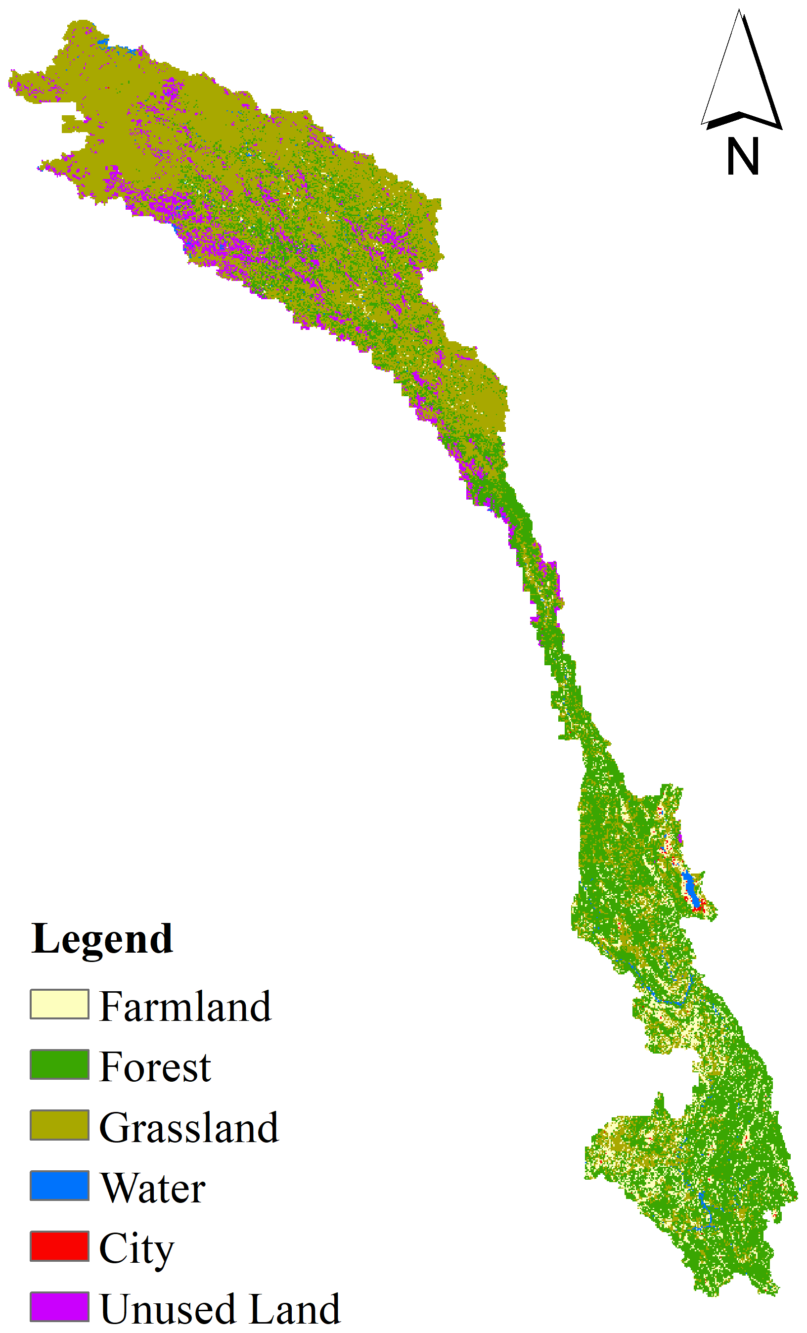
Figure 16 Land use classification in the LR basin in 2015.

5.3 Comparison with results of other published studies

As analyzed above, there was no particularly significant change in the precipitation and potential evapotranspiration from 1961 to 2015 in the LR basin. HAs mainly included the construction of reservoirs, resulting in changes in the streamflow. Attribution analysis results showed that the CR of HAs was 57.6 %, and the corresponding CC was 42.4 %. This result was basically consistent with Han et al. (2019), but the CR of HAs was smaller than that of calculation results. This may be due to the following reasons.

1. The streamflow data of different time spans were used to obtain different break points. They used streamflow data from 1980 to 2014 to obtain the break point in 2008, and this study used data from 1961 to 2015 to identify the break point in 2005.

2. Different hydrological models were used. They used the coupled routing and excess storage (CREST) model with an NSE of 0.57, while the SWAT model used in this study had an NSE of 0.94.

3. Longer series of streamflow data and simulation data were used.

As indicated by D. Li et al. (2017) and Han et al. (2019), as the streamflow data series became longer in the impacted period, the impact of reservoir scheduling on the streamflow changes on an average scale for many years gradually decreased. D. Li et al. (2017) selected Chiang Saen station, which was the nearest station to Yunjinghong station downstream of the LR basin, for their research, and then they divided the streamflow series into three stages, the pre-impact period (1960–1991), the transition period (1992–2009), and the post-impact period (2010–2014). They concluded that the construction of the reservoirs in the LR basin led to a decrease in the streamflow process during the flood period and an increase in the dry period, which was consistent with the results of our study (Sect. 4.3.2). Their results also showed that HAs contributed 61.88 % to the streamflow reduction at Chiang Saen station, which was also close to the results of our study (57.4 %).

5.4 Applicability and uncertainty of the proposed framework

A new quantitative framework for calculating the CR of CC and HAs to watershed streamflow variations was proposed in this study, and it was successfully applied to the LR basin with relatively accurate results. From our perspective, this method can effectively quantify the influence of the “equifinality for different parameters” that may exist in the use of hydrological simulation methods to quantify the CR of CC and HAs. At the same time, we also believe that this framework can be applied to other watersheds based on the following aspects. First, in Sect. 4.4, the Budyko framework and sectional water withdrawal data within the basin were used to compare with the new framework. Second, the results of the comparison with published research on the LR basin (Han et al., 2019) also proved that the framework has good accuracy and applicability. Third, in the process of comparing with the new framework, we fully considered the impact of various HAs within the study area, including five types of water withdrawals (i.e., irrigation, livestock, living, mining, and manufacturing) and the impact of reservoir storage and the land use/land cover change. Of course, due to the highly nonlinear relationship between the parameters of the hydrological model, we suggest that readers ensure that the selected simulation results with NSEs greater than 0.75 are large enough when applying the novel framework in other research areas (this study had 500 simulations). It is undeniable that this method still has certain uncertainties and limitations when it is applied to other watersheds. First, if there are multiple break points in the annual streamflow sequence, then, when selecting the unique break point, it is necessary to consider the abrupt change points of the time series of other meteorological elements (precipitation, temperature, etc.) in the basin. At the same time, the impact of strong human activities (reservoir construction, large-scale water transfer project construction, etc.) on the abrupt change of streamflow in the basin should also be considered (Dey and Mishra, 2017). Finally, a unique break point is selected to divide the research time series into a natural period and an impacted period, and then the quantitative framework proposed in this study can be applied. Second, because the SWAT model has good applicability at the Yunjinghong station in the LR basin, it can meet the 500 best simulation requirements set by the framework proposed in this study, but the hydrological model may have different applicability in different research areas. Therefore, the application of this framework in other research areas may have limitations, which needs to be further verified. Third, because this study uses the parameter combinations obtained by the natural period to input the meteorological element data of the impacted period for calculation, this may also bring uncertainty to the calculation results, which is usually called “transferability” (Fu et al., 2018).

Although the new quantitative framework proposed in this study considers the uncertainties in hydrological simulations, the framework is still based on traditional hydrological simulation methods to separate the CR of CC into streamflow change and then to deduce the CR of HAs. Therefore, inevitably, there are still uncertainties in the calculation process. For example, the construction of large-scale reservoirs and changes in land use/land cover (urbanization, etc.) are important factors that alter the climatic state of a local region, specifically in that they change the temporal and spatial distribution characteristics of local regional hydrometeorological elements (Y. Li et al., 2017; Degu et al., 2011). This change in meteorological elements was regarded as part of the impact of CC in this study; however, it was also caused by both HAs (reservoir construction) and CC. On the other hand, there are uncertainties in the division of the natural period and the impacted period in this study, which assumed that the impact of HAs on streamflow changes in the natural period was negligible; however, there were almost no periods within a watershed that were completely unaffected by HAs, and the impact of HAs on streamflow variations in the natural period was ignored in these studies. In this study, there was also a strong disturbance of HAs during the natural period (i.e., reservoir construction: Manwan and Dachaoshan) (Table 1). In addition, our study selected the NSE as the objective function to calibrate the SWAT model, which may also bring uncertainties in the quantitative results. As indicated by Gupta et al. (2009) and Gupta and Kling (2011), using the NSE as an objective function to calibrate a hydrological model may tend to underestimate the peak streamflow. Although the CR in our study was calculated by the average streamflow over multiple years, it still brought a given amount of uncertainty to the quantitative results. Therefore, follow-up research should strengthen the optimization of the objective function and benefit from field investigation of the actual meaning of the parameters. Since the impacts of CC and HAs on the hydrological processes of the watershed are complicated and interconnected, it is still a challenge to completely separate the impacts of CC and HAs on streamflow variations (Xin et al., 2019). Further consideration should be given to quantifying the impact of specific HAs, such as land use change and water withdrawal, and then to separating the impact of CC and HAs on streamflow changes as completely as possible.

6 Conclusions

In this study, we proposed a new framework that considered the uncertainties of model simulations to quantify the CR of CC and HAs to streamflow changes. This framework was developed based on the posterior histogram frequency distribution (PHD) of the CR of CC and HAs. Then, we selected the LR basin for the case study. Over the past 3 decades, after the construction of the Manwan Reservoir in 1987, six large reservoirs were constructed within the basin before 2014. The streamflow process in the watershed also has significant changes on multiyear average and monthly scales. The Mann–Kendall monotonic trend test and the Mann–Kendall break point test were used to test the trend and identify the break point of the annual streamflow data at Yunjinghong station within the period of 1961 to 2015. Then, the available period was divided into the natural period (before the break point) and the impacted period (after the break point). Afterwards, the SWAT model and the SUFI-2 method were used to construct the posterior histogram distribution (PHD) of the CR of CC and HAs. Finally, the Budyko framework and the basin-wide gridded monthly sectoral water use (GMSWU) data set were used to compare with the newly proposed framework. The main conclusions of this study are as follows.

1. The new proposed framework can be used to quantify the CR of CC and HAs in the LR basin which can fully solve the local optimal solution for hydrological simulation parameters in current related studies. The results of comparison using the Budyko framework and Gridded Monthly Sectoral Water Use (GMSWU) data set also showed that the new framework has high accuracy (the error range is within 6 %).

2. The break point of the streamflow sequence during 1961–2015 at Yunjinghong station was identified in 2005. The streamflow significantly decreased (∼ −22 %) after 2005 compared with that of the natural period (1961–2004), which was mainly due to the construction of the Xiaowan Reservoir in October 2004. Significantly reduced streamflow in the flood period and significantly increased streamflow during the dry period also occurred, which was mainly due to the capacity adjustment of the constructed reservoirs. The trend test results also showed that from 1961 to 2015, the annual streamflow in the LR basin showed a significant decreasing trend at the α= 0.01 significance level, precipitation showed a nonsignificant decreasing trend, and mean temperature showed a significant increasing trend at the α= 0.01 significance level.

3. The quantification results calculated using the new proposed framework showed that, on an annual scale, compared with the natural period of 1961–2004, the CR of CC and HAs (CR of CC and HAs) were 40 %–45 % (with an average CR of 42.6 %) and 55 %–60 % (with an average CR of 57.4 %), respectively. The CR of CC and HAs derived from the Budyko framework were 37.2 % and 62.8 %, respectively, and the error between the two calculation results was 5.4 %. The CR of HAs calculated using the GMSWU data and the reservoirs dead capacities was 58.0 %, which also proved that the new proposed framework in this study can be used in the LR basin.

4. Quantitative analysis results on a monthly scale in the LR basin showed that, except for June and November, streamflow changes in other months were caused by HAs. Further analysis showed that the streamflow in June during the impacted period decreased by 6.9 mm compared with that in the natural period, while the precipitation and potential evapotranspiration decreased and increased by 20.2 and 8.83 mm, respectively; the streamflow decreased by 5.34 mm in November, while the corresponding precipitation and potential evapotranspiration changed by −7.43 and 5.52 mm, respectively.

In summary, this study provides a new calculation framework that considers the uncertainty of hydrological simulations to quantify the CR of CC and HAs to streamflow changes. The results of this case study also provide a reference for understanding the dominant factors of streamflow changes in the LR basin and improving water resource management measures for the transboundary Lancang–Mekong River basin. Of course, this new proposed framework also needs to be applied and verified in more research areas. In addition, this framework only considers the dual impacts of CC and HAs. However, in practical applications, water resource decision-makers are more willing to understand the specific impacts of HAs such as irrigation water and land use changes. Therefore, in future research, efforts should be made to expand the framework to quantify the CRs of individual items of CC and HAs.

Appendix A: Abbreviations

AE	Actual evaporation
CC	Climate change
CGDPA	China gauge-based daily precipitation analysis
CMA	China Meteorological Administration
CR	Contribution rate
CREST	Coupled routing and excess storage
DEM	Digital elevation model
GMSWU	Global gridded Monthly Sectoral Water Use data set
HA	Human activity
HRU	Hydrologic response unit
HWSD V1.2	Harmonized World Soil Database Version 1.2
LR	Lancang River
NSE	Nash–Sutcliffe efficiency coefficient
PET	Potential evapotranspiration
PHD	Posterior histogram distribution
RE	Relative error
SRTM	Shuttle Radar Topography Mission
SUFI-2	Sequential Uncertainty Fitting Procedure version 2
SWAT	Soil and Water Assessment Tool
USDA	US Department of Agriculture Research Service