Probabilistic subseasonal precipitation forecasts using preceding atmospheric intraseasonal signals in a Bayesian perspective

Accurate and reliable subseasonal precipitation forecasts are of great socioeconomic value for various aspects. The atmospheric intraseasonal oscillation (ISO), which is one of the leading sources of subseasonal predictability, can potentially be used as predictor for subseasonal precipitation forecasts. However, the relationship between atmospheric intraseasonal signals and subseasonal precipitation is of high uncertainty. In this study, we develop a spatiotemporal-projection-based Bayesian hierarchical model (STP-BHM) for subseasonal precipitation forecasts. The coupled covariance patterns between the preceding atmospheric intraseasonal signals and precipitation are extracted, and the corresponding projection coefficients are defined as predictors. A Bayesian hierarchical model (BHM) is then built to address the uncertainty in the relationship between atmospheric intraseasonal signals and precipitation. The STP-BHM model is applied to predict both the pentad mean precipitation amount and pentad mean precipitation anomalies for each hydroclimatic region over China during the boreal summer monsoon season. The model performance is evaluated through a leave-1-year-out cross-validation strategy. Our results suggest that the STP-BHM model can provide skillful and reliable probabilistic forecasts for both the pentad mean precipitation amount and pentad mean precipitation anomalies at leads of 20–25 d over most hydroclimatic regions in China. The results also indicate that the STP-BHM model outperforms the National Centers for Environmental Prediction (NCEP) subseasonal to seasonal (S2S) model when the lead time is beyond 5 d for pentad mean precipitation amount forecasts. The intraseasonal signals of 850 and 200 hPa zonal wind (U850 and U200) and 850 and 500 hPa geopotential height (H850 and H500) contribute more to the overall forecast skill of the pentad mean precipitation amount predictions. In comparison, the outgoing longwave radiation anomalies (OLRAs) contribute most to the forecast skill of the pentad mean precipitation anomaly predictions. Other sources of subseasonal predictability, such as soil moisture, snow cover, and stratosphere–troposphere interaction, will be included in the future to further improve the subseasonal precipitation forecast skill.

1 Introduction

Accurate and reliable subseasonal precipitation forecasts can provide vital information for many management decisions in water resources, agriculture, and disaster mitigation (Vitart et al., 2012; Vitart and Robertson, 2018). One approach for subseasonal precipitation forecasts is to run dynamical models such as global climate models (GCMs). Projects such as the Subseasonal to Seasonal Prediction (S2S) Project and the Subseasonal Experiment (SubX) have been launched to provide subseasonal precipitation forecasts with lead time of up to 60 d from GCMs (Pegion et al., 2019; Vitart et al., 2017). However, the subseasonal precipitation forecasts derived directly from GCMs are of low accuracy as the physical equations are always simplified, and small-scale processes cannot be well represented in the GCMs (De Andrade et al., 2019). Post-processing is always required to improve the accuracy and reliability of GCM forecasts before they can be used for other applications. Schepen et al. (2018) and our previous study (Li et al., 2020) used the Bayesian joint probability (BJP) method to post-process subseasonal precipitation forecasts over different regions, and the results suggested that the forecast skill and reliability were improved compared to raw GCM forecasts. Vigaud et al. (2020) proposed a new spatial correction method to improve submonthly precipitation forecasts derived from multimodel ensembles. Nevertheless, the results also indicated that the accuracy of post-processed subseasonal precipitation forecasts were still limited when the lead time was beyond 10–14 d.

An alternative approach for subseasonal precipitation forecasts is to establish statistical models based on the relationship between precipitation and preceding atmospheric or oceanic indices. Although dynamical models perform better for short- to medium-term forecasts, statistical models are still found to be useful, especially for long-term forecasts (Tuel and Eltahir, 2018; Abbot and Marohasy, 2014; Mekanik et al., 2013; Lü et al., 2011; Kirono et al., 2010). Schepen et al. (2012) suggested that the lagged climate indices were potentially useful for seasonal precipitation forecasts over Australia. Plenty of statistical algorithms, such as multiple linear regression or canonical correlation analysis, have been developed for seasonal precipitation forecasts based on the assumption that the seasonal anomalies are caused by slow-varying sea surface temperature, sea ice, snow cover, and other boundary conditions (Hwang et al., 2001; Barnston and Smith, 1996; Eden et al., 2015). A new cluster-based empirical method was proposed to predict winter precipitation anomalies over the European and Mediterranean regions (Totz et al., 2017). This method used the sea surface temperature, geopotential height, sea level pressure, snow cover extent, and sea ice concentration as predictors. A random-forest-based statistical model, whose the predictors were identified from the gridded sea surface temperature, was developed to predict central and south Asian seasonal precipitation (Gerlitz et al., 2016).

However, much fewer statistical models have been built and applied for subseasonal precipitation forecasts, as the sources of subseasonal predictability are not yet fully understood. Compared to seasonal precipitation forecasts, the slow-varying boundary forcings may have limited impact on subseasonal precipitation as the timescale is too short. The atmospheric intraseasonal oscillation (ISO), which is the dominant mode of the subseasonal variability, is one of the leading sources of subseasonal predictability (Robertson and Vitart, 2018). The boreal summer intraseasonal oscillation (BSISO) in the tropics, which is also known as Madden–Julian Oscillation (MJO) in winter, is characterized as a slow-moving system with a period of 30–90 d in the tropical atmosphere (Madden and Julian, 1971, 1972; Zhang, 2005; Woolnough, 2019; Wang and Xie, 1997). The circulation anomalies associated with the intraseasonal oscillation (ISO) are identified to have an impact on monsoon activities and heavy rainfall events (Annamalai and Slingo, 2001; Chen et al., 2004). Zhang et al. (2009) found that the rainfall patterns in southeastern China were transited from being enhanced to being suppressed when the MJO center moved from the Indian Ocean to the western Pacific Ocean. Jia et al. (2011) suggested that the MJO influenced the rainfall patterns in China mainly by modulating the circulation in the subtropics and mid–high latitudes in winter. This suggests that the ISO signals could be potentially used for predicting subseasonal precipitation not only in tropical regions but also in extra-tropical regions.

Several statistical models have been built to predict subseasonal precipitation based on the relationship between atmospheric intraseasonal signals and precipitation. The spatiotemporal projection (STP) model, which extracts the coupled patterns of the predictors and the predictand, has been developed in recent years (Hsu et al., 2020; Zhu and Li, 2017c, a, b, 2018). Hsu et al. (2015) established a set of spatiotemporal projection models (STPMs) to predict subseasonal precipitation at a lead time of 10–30 d over southern China. Their results suggested that the forecast skill was still promising at a 20–25 d lead time. Zhu and Li (2017c) predicted subseasonal precipitation by constructing STPMs over the whole of China, and independent forecasts of rainfall anomalies during the period of Olympic Games in 2008 and Shanghai World Expo in 2010 suggested that the STPMs were able to reproduce intraseasonal rainfall patterns at a 20 d lead time. However, we should note that the relationship between ISO signals and precipitation is highly uncertain and depends on the region and lead time. In previous studies, an optimal ensemble (OE) strategy was applied to generate probabilistic forecasts by picking up the best predictors (Zhu and Li, 2017c; Zhu et al., 2015). Nevertheless, the number of best predictors was always limited. Further statistical assumptions were required to interpret limited ensembles as probabilistic forecasts. The uncertainty in relationship between preceding ISO signals of atmospheric field and precipitation has not been fully considered yet.

There are several ways to address the above challenge. Lepore et al. (2017) established an extended logistic regression model to link the relationship between the El Niño–Southern Oscillation (ENSO) and convective storm activity. Sohrabi et al. (2021) coupled the large-scale climate indices with a stochastic weather generator to provide ensemble streamflow forecasts. Compared to the above-mentioned traditional probabilistic model solutions, the Bayesian statistical models are more flexible and more efficient for assessing multiple sources of uncertainties. Wang et al. (2009) proposed a multivariate normal-distribution-based Bayesian joint probability (BJP) approach to predict seasonal streamflow over Australia using antecedent streamflow, ENSO indices, and other climate indicators as predictors. Peng et al. (2014) utilized the same BJP approach to predict seasonal precipitation over China using lagged oceanic–atmospheric indices. The Bayesian hierarchical model (BHM) has also been developed in recent years (Gelman and Hill, 2006). The BHMs are always constructed with several model layers. The predictand is assumed to follow a distribution with unknown parameters in the first layer, and the parameters are linked with the predictors, using linear regression models, in the second layer. The regression coefficients are given hyperprior distributions with the BHMs. The utility of BHMs has been demonstrated in modeling the spatiotemporal variability in hydrological variables in many studies (Renard, 2011; Reza Najafi and Moradkhani, 2013; Bracken et al., 2016; Lima and Lall, 2009, 2010; Devineni et al., 2013). The BHMs are also used for seasonal predictions in many fields. Chen et al. (2014) used the BHM to predict summer rainfall and streamflow over the Huai River basin, while Chu and Zhao (2007) developed a BHM model to predict seasonal tropical cyclone activity over the central North Pacific. However, the BHMs have not been used to predict subseasonal precipitation before. In this study, we follow a similar BHM structure to that proposed by Devineni et al. (2013) to predict subseasonal precipitation.

China is located in East Asia and is frequently subject to rainstorm and flood disasters during the boreal summer monsoon season. Accurate and reliable subseasonal precipitation forecasts can provide valuable information for mitigating the risks from rainstorm and flood disasters. However, the origin of intraseasonal precipitation variability is of high complexity owing to the mixed impact of tropical convection, forcing of Tibetan Plateau, and mid–high latitude systems (Zhu and Li, 2017c). In this study, we develop a spatiotemporal-projection-based Bayesian hierarchical model (STP-BHM) to predict both the pentad mean precipitation amount and pentad mean precipitation anomalies over each hydroclimatic region in China during the boreal summer monsoon season. The performance of the STP-BHM model is evaluated through a leave-1-year-out cross-validation strategy.

In the following section, the datasets, main model components (including intraseasonal signal extraction, predictor definition, and Bayesian hierarchical model construction), and verification methods are introduced. The forecast skill of both the pentad mean precipitation amount and pentad mean precipitation anomalies is presented in Sect. 3. Section 4 discusses the forecast skill, possible mechanism, limitations, and future work. Key findings are summarized in Sect. 5.

2 Data and methodology

2.1 Data

In this study, China is divided into 17 hydroclimatic regions, as suggested by Lang et al. (2014). The division is based on both the watershed division standard and climate classifications. This will ensure that the climatic characteristics are nearly uniform in each region. The southeastern hydroclimatic regions are mostly of a temperate and warm/hot summer climate without a dry season (Cfb/Cfa), while the northwestern regions are mostly arid with limited precipitation (Bwk, Bsh, and Bsk climate types; Peel et al., 2007; Fig. 1). The observed precipitation is derived from the Multi-Source Weighted-Ensemble Precipitation, version 2 (MSWEP V2), dataset. The MSWEP V2 dataset is of a high spatial (0.1^∘) and temporal (3 h) resolution. Compared to other gridded datasets, MSWEP V2 exhibits more realistic spatial patterns and higher accuracy over land (Wu et al., 2018; Beck et al., 2019). The 0.1^∘ gridded precipitation data are area-weighted and averaged through 17 hydroclimatic regions over China from May to October.

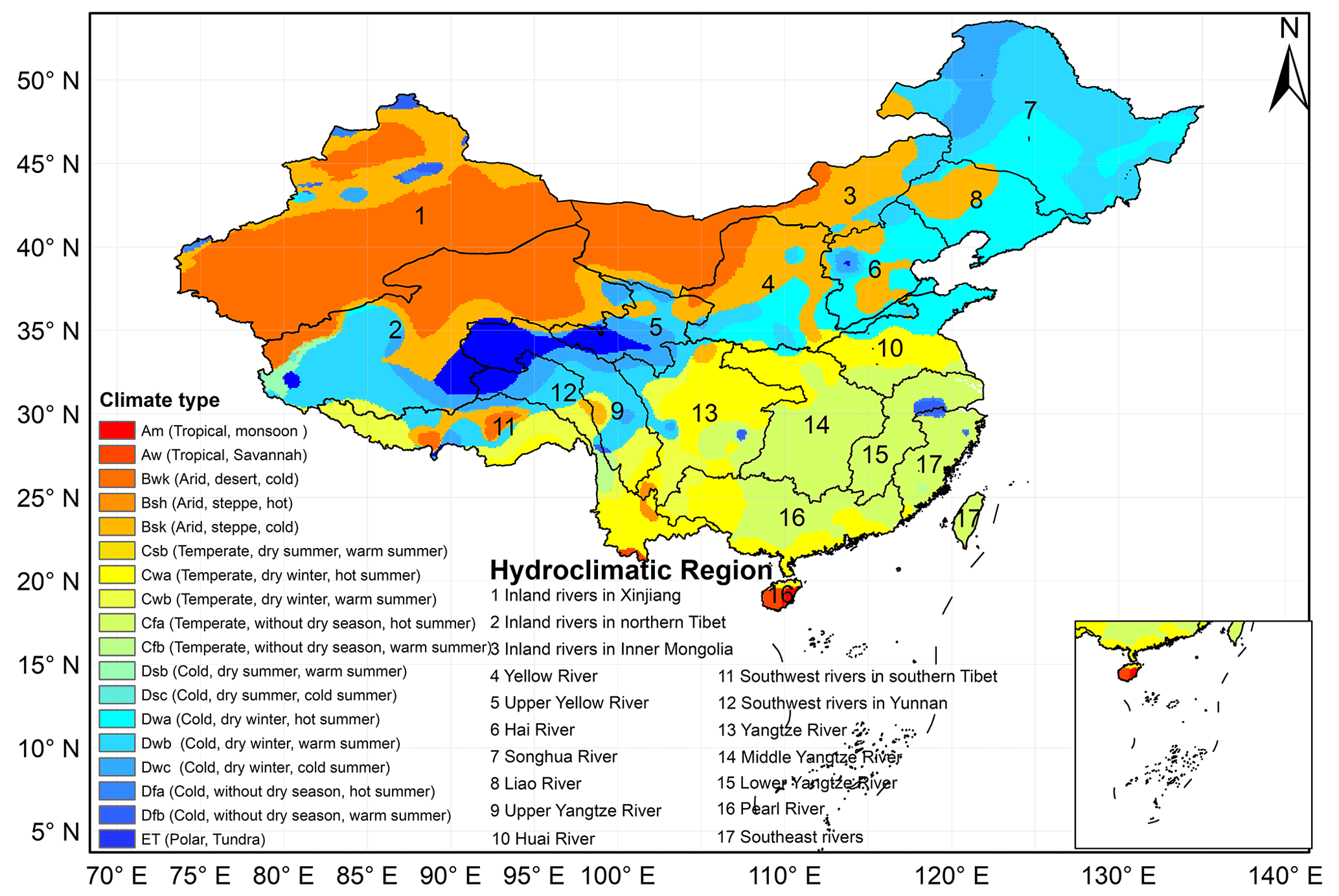
Figure 1 The 17 hydroclimatic regions over China.

The intraseasonal oscillation is always represented by outgoing longwave radiation (OLR) and zonal winds in the upper (200 hPa) and lower (850 hPa) troposphere. Although several indices, including the RMM (real-time multivariate MJO) index (Wheeler and Hendon, 2004) and BSISO index (Lee et al., 2013), have been proposed to monitor the propagation of the oscillation, these indices may not cover patterns which might be important for subseasonal precipitation in certain regions. To overcome this problem, we analyze the correlation between the ISO signals of the preceding global OLR, zonal wind at 850 hPa (U850), zonal wind at 200 hPa (U200), and precipitation for each grid cell. In addition, the correlations with geopotential height at 850, 500, and 200 hPa (H850, H500, and H200) are also analyzed. The H850, H500, and H200 values have been proved to be as capable of reflecting the MJO structure as the zonal wind (Leung and Qian, 2017). The OLR data used in this study are derived from National Climatic Data Center (NCDC) on a 1.0^∘ squared resolution over the globe. The OLR data are developed from high-resolution infrared radiation sounder instruments and are valuable for a wide range of applications. A more detailed description of the OLR dataset can be found at https://www.ncei.noaa.gov/access/metadata/landing-page/bin/iso?id=gov.noaa.ncdc:C00875, last access: 24 December 2021). The global gridded daily average U850, U200, H850, H500, and H200 data are derived from the ERA5 reanalysis dataset at https://cds.climate.copernicus.eu/ (last access: 24 December 2021). The ERA5 reanalysis dataset is produced using advanced 4D-Var data assimilation scheme, and its horizontal resolution is approximately 30 km, with 137 pressure levels in the vertical (Hersbach et al., 2020). It provides an hourly record of global atmosphere, land surface, and ocean waves from 1950 to present. To focus on large-scale features and increase the computational efficiency, both the OLR data and the ERA5 reanalysis data are bilinearly interpolated onto $\mathrm{2.5}{}^{\circ }\times \mathrm{2.5}{}^{\circ }$ latitude–longitude resolution. Moreover, we choose to focus on the period of 1979–2016 to be consistent with the temporal coverage of the observed precipitation data.

The STP-BHM model we built in this study is compared to the dynamical models to provide a benchmark for subseasonal precipitation forecasts. In this study, we compare our results of the STP-BHM model with the National Centers for Environmental Prediction (NCEP) model archived in the S2S database for the same period of 1999–2010, from May to October (http://apps.ecmwf.int/datasets/data/s2s/, last access: 24 December 2021). The NCEP hindcasts are produced by the Climate Forecast System Version 2 (CFSv2), which is composed of land, ocean, and atmosphere components. The system provides a four-member ensemble that is run every day from 1 January 1999 to 31 December 2010. More details on the NCEP hindcasts are available at https://confluence.ecmwf.int/display/S2S/NCEP+Model+Description (last access: 1 July 2022). The pentad mean precipitation amount forecasts of the NCEP model are generated to be consistent with the STP-BHM model.

2.2 Methodology

2.2.1 Modeling structure

The spatiotemporal-projection-based Bayesian hierarchical model (STP-BHM) consists of three parts, as shown in Fig. 2. The first part (Sect. 2.2.2) extracts the intraseasonal signals of each global atmospheric field (U850, U200, OLR, H850, H500, and H200) and precipitation, using a non-filtering method proposed by Hsu et al. (2015). In the second part (Sect. 2.2.3), the cell-wise correlation between the ISO signals of atmospheric field and precipitation is analyzed in the six preceding pentads. The spatiotemporal coupled covariance patterns are constructed for grid points where the correlation is statistically significant at the 5 % level. The predictor is then defined by summing the product of the covariance field and atmospheric intraseasonal signals of atmospheric field at each preceding pentad. In the statistical modeling step (Sect. 2.2.4), both predictors and the predictand are transformed to follow normal distributions. A Bayesian hierarchical model is then built to address the uncertainty in the relationship between the predictors and predictand. The model is applied to generate probabilistic subseasonal precipitation forecasts after parameter inference.

Figure 2 Workflow of the spatiotemporal-projection-based Bayesian hierarchical model (STP-BHM).

2.2.2 Intraseasonal signal extraction

As briefly introduced in the previous section, extracting meaningful intraseasonal signals is important for subseasonal precipitation forecasts. However, high-frequency (unpredictable) noise exists for both raw daily atmospheric variables (U850, U200, OLR, H850, H500, and H200) and raw daily precipitation. Band-pass filtering methods, such as the fast Fourier transformation, are always used to isolate intraseasonal low-frequency (10–60 d) signals from raw data (Zhang, 2005). However, a traditional band-pass filtering method is impractical for real-time applications as future information beyond the current date is needed. In this study, a non-filtering method proposed by Hsu et al. (2015) is used to extract 10–60 d signals of both atmospheric variables and precipitation. Compared to the traditional intraseasonal signal extraction method, this approach is easy to implement and could be used for real-time applications. The climatological annual cycle of the raw daily data is first removed by subtracting a 90 d low-pass filtered climatological component, as follows:

$$\begin{array}{}\text{(1)}& X^{\prime }=X-\stackrel{\mathrm{‾}}{X},\end{array}$$

where X is the raw daily data of the atmospheric field or precipitation. $\stackrel{\mathrm{‾}}{X}$ is the corresponding climatological 90 d low-pass filtered component derived by the Lanczos filtering method during the period of 1981–2010 (Duchon, 1979). In the second step, lower-frequency signals longer than 60 d are removed by subtracting the running mean of the last 30 d, as follows:

$$\begin{array}{}\text{(2)}& X^{\prime \prime }=X^{\prime }-{\stackrel{\mathrm{‾}}{X^{\prime }}}^{\text{30\hspace{0.17em}d}},\end{array}$$

where ${\stackrel{\mathrm{‾}}{X^{\prime }}}^{\text{30\hspace{0.17em}d}}$ is the running mean of the last 30 d of X^′.

The higher-frequency signals are then removed by taking a pentad mean, as follows:

$$\begin{array}{}\text{(3)}& X^{\ast }={\stackrel{\mathrm{‾}}{X^{\prime \prime }}}^{\text{5\hspace{0.17em}d}}.\end{array}$$

The so-derived variable represents the 10–60 d signals of the daily atmospheric field or precipitation. The daily intraseasonal signals are then averaged to pentad data to further reduce the noise and improve the predictability. The pentad mean 10–60 d signal of precipitation is also referred to as the pentad mean precipitation anomalies in the following sections.

2.2.3 Predictor definition

To identify relevant areas of atmospheric fields that could affect the 10–60 d precipitation variability, we analyze the correlation between the preceding 10–60 d signals of atmospheric fields and precipitation for each hydroclimatic region during the period of 1979–2016, from May to October. Owing to the data persistence introduced by the filtering method, the effective degree of freedom for each grid cell and each preceding pentad is estimated following Livezey and Chen (1983).

As an example, Figs. 3 and 4 present the correlation between the preceding pentad mean 10–60 d signals of U850, U200, OLRAs, H850, H500, and H200 and precipitation over Region 1 (inland rivers in Xinjiang) at different lead times. At leads of 25 to 20 d, the significantly correlated U850 signals are mainly over the western Indian Ocean. The U850 signals are then propagating eastward toward the equatorial Indian Ocean at leads of 15 to 10 d. The U850 anomalies then gradually moved eastward and northward toward western Pacific Ocean, Mongolian Plateau, Iranian plateau, and Qinghai–Tibet Plateau from the lead of 10 to 0 d. The U200 signals are more pronounced compared to the U850 signals. The spatial distribution of potential predictive U200 regions is rather concentrated, indicating more robust statistical relationships. The OLR anomalies appear near the Bay of Bengal at 20 to 15 d leads. At leads of 5 to 0 d, the significantly correlated OLR signals are mainly over the eastern European Plain and West Siberian Plain.

Figure 3 Correlation coefficient between the preceding pentad mean 10–60 d signals of U850, U200, outgoing longwave radiation anomalies (OLRAs), and precipitation over Region 1 (inland rivers in Xinjiang) at different lead times during the period of 1979–2016, from May to October. Correlation coefficients that are statistically significant at the 5 % level are shaded.

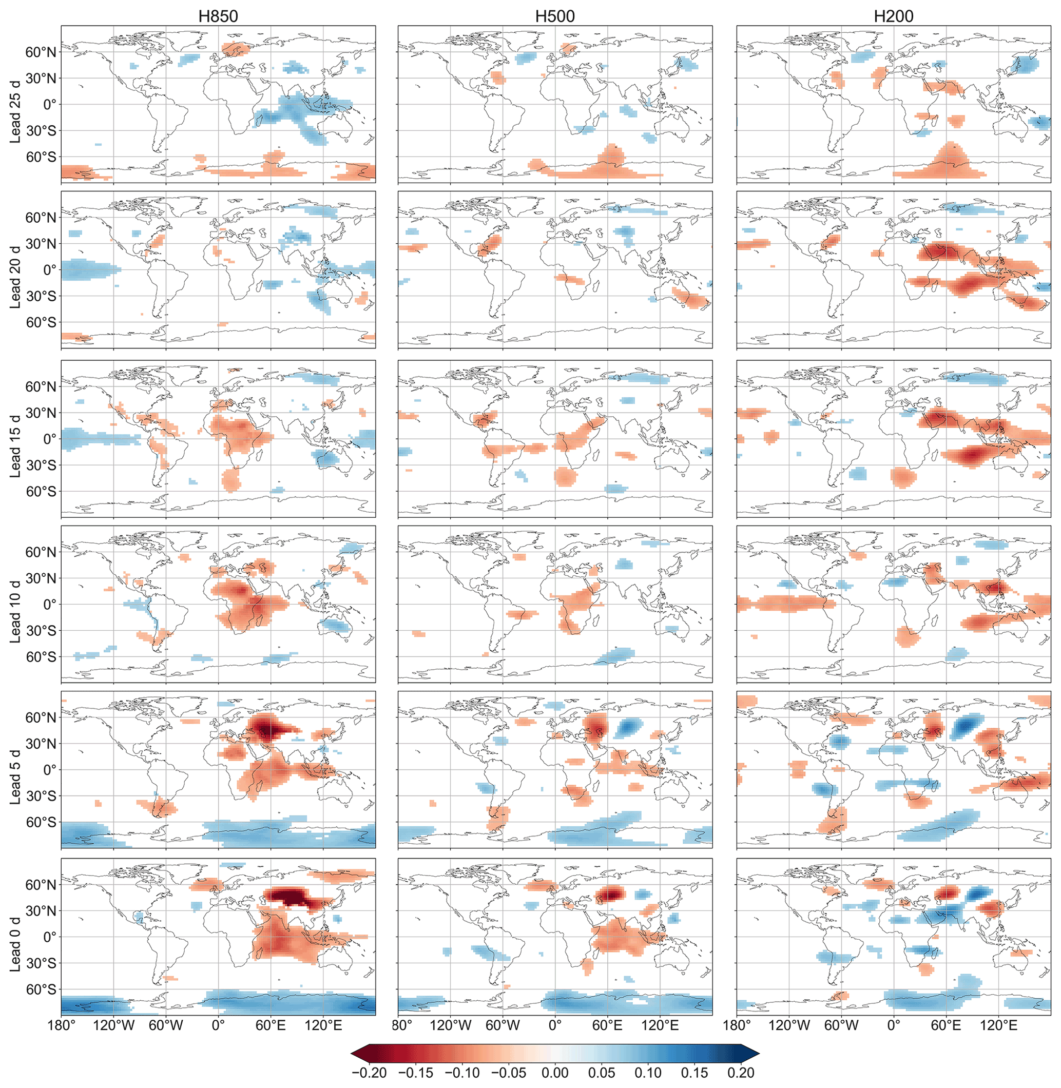
Figure 4 Same as Fig. 3 but for H850, H500, and H200.

The H850 anomalies appear near the equatorial Indian Ocean and Philippine Sea at lead times of 25 to 20 d. At leads from 15 to 20 d, the significantly correlated H850 signals are mainly over Africa. The signals gradually move eastward and northward toward Indian Ocean, Iranian Plateau, and central Asia from lead times of 10 to 0 d. Unlike the H850 fields that originated over Africa, the H200 anomaly appears to originate from the Arabian Sea, southern Indian Ocean, and western Pacific Ocean from leads of 25 to 15 d. At lead times of 10 to 0 d, the significantly correlated H200 signals are mainly over eastern European Plain, West Siberian Plain, and Central Siberian Plateau.

The correlation maps between preceding pentad mean 10–60 d signals of U850, U200, outgoing longwave radiation anomalies (OLRAs), H850, H500, and H200 and precipitation over other regions are presented in Figs. S1 to S32 in the Supplement.

The spatiotemporal coupled covariance patterns are then constructed for a grid point where the correlation is statistically significant at the 5 % level. The predictor is then defined by summing the product of the covariance patterns and ISO signals of atmospheric field at each preceding pentad, as follows:

$$\begin{array}{}\text{(4)}& {\displaystyle }\text{cov}(X_{i,p},Y)={\displaystyle \frac{\mathrm{1}}{T}}\sum _{t=\mathrm{1}}^T(y_t-E(y\left)\right)(x_{i,p,t}-E(x_{i,p}\left)\right)\text{(5)}& {\displaystyle }{X}_p=\sum _{i=\mathrm{1}}^N\text{cov}(X_{i,p},Y)\cdot X_{i,p},\end{array}$$

where X_i,p denotes the pentad mean 10–60 d signal of the pth atmospheric field where the correlation is statistically significant at the 5 % level for grid i, $p=\mathrm{1},\mathrm{2},\mathrm{\dots },\mathrm{6}$. Y denotes the pentad mean precipitation amount or pentad mean precipitation anomalies. T is the total number of pentads, and N is the total number of grid points at which the correlation is statistically significant at the 5 % level. Thus, there is only one predictor X_p for each atmospheric field and each preceding pentad.

2.2.4 Statistical modeling

In previous steps, we defined the predictors by analyzing the relationship between the ISO signals of the atmospheric field and precipitation. The so-derived predictors can be used to predict the pentad mean precipitation amount and the pentad mean precipitation anomalies. Consider, for example, predicting the pentad mean precipitation amount for the period between 1 and 5 May 1979. In this case, the pentad mean ISO signals of the atmospheric field on 26–30, 21–25, 16–20, 11–15, 6–10, and 1–5 April 1979 are used as predictors to generate precipitation forecasts at different lead times. A leave-1-year-out cross-validation strategy is implemented for data normalization, model building, parameter inference, and verification to avoid any bias in skill (Michaelsen, 1987). For instance, to produce subseasonal precipitation forecasts in 1979, the predictors (preceding ISO signals) and predictand (pentad mean precipitation) during the period of 1980–2016 are pooled together for statistical modeling. The forecasts for the year 1979 are then issued by models trained on 1980–2016, and the performance is evaluated against the observations. This cross-validation strategy ensures that the data used for the evaluation are never used for statistical modeling.

Before establishing the Bayesian hierarchical model, the predictors X^T=[X₁X₂⋯X_P] are normalized to ${\mathit{X}}_{\text{norm}}^T=\left[X_{\text{norm},\mathrm{1}}{X}_{\text{norm},\mathrm{2}}\mathrm{\cdots }{X}_{\text{norm},P}\right]$ through the Yeo–Johnson transformation method, as the input variables are allowed to be negative (Yeo and Johnson, 2000). The predictand Y is normalized to Y_norm, using the Yeo–Johnson method for pentad mean precipitation anomalies. However, the pentad mean precipitation amount is highly skewed with numerous zero values. Here, we normalize the pentad mean precipitation amount Y to Y_norm, using the log-sinh transformation method proposed by Wang et al. (2012). The normalization parameters are estimated using the SCE-UA (shuffled complex evolution method developed at the University of Arizona) method that maximizes the log-likelihood function for both the Yeo–Johnson transformation method and log-sinh transformation method.

There are many versions and variations in BHMs. In this study, we establish the BHM model following Devineni et al. (2013) and Chen et al. (2014). The spatial correlation of precipitation over different regions is not considered here. A traditional no-pooling BHM is built for each hydroclimatic region separately. The normalized predictand Y_norm is assumed to follow the normal distribution, as follows:

$$\begin{array}{}\text{(6)}& Y_{\text{norm}}\sim N(\mathit{\mu },{\mathit{\sigma }}^{\mathrm{2}}).\end{array}$$

We then link the parameter μ with the normalized predictors, using a linear model, as follows:

$$\begin{array}{}\text{(7)}& \mathit{\mu }={\mathit{\beta }}_{\mathrm{0}}+\sum _{p=\mathrm{1}}^P{\mathit{\beta }}_p{X}_{\text{norm},p},\end{array}$$

where β_p is the slope term corresponding to the normalized predictor X_norm,p, and P is the total number of predictors used for prediction.

To complete the hierarchical formulation, we assume that the unknown parameters, including $\mathit{\sigma },{\mathit{\beta }}_{\mathrm{0}},\mathrm{\dots },{\mathit{\beta }}_P$, follow these non-informative priors, as follows:

$$\begin{array}{}\text{(8)}& {\displaystyle \frac{\mathrm{1}}{{\mathit{\sigma }}^{\mathrm{2}}}}\sim U(\mathrm{0},\mathrm{100})\text{(9)}& {\displaystyle }{\mathit{\beta }}_{\mathrm{0}}\sim N(\mathrm{0},{\mathrm{10}}^{\mathrm{4}})\text{(10)}& {\displaystyle }{\mathit{\beta }}_p\sim N(\mathrm{0},{\mathrm{10}}^{\mathrm{4}}),p=\mathrm{1},\mathrm{\dots },P.\end{array}$$

This implies that the information used for a posterior distribution inference is only provided by the data.

Given that $\mathit{\theta }=\mathit{\left\{}\right(\mathit{\sigma },{\mathit{\beta }}_{\mathrm{0}},{\mathit{\beta }}_p)$, $p=\mathrm{1},\mathrm{\dots },P\mathit{\}}$ denotes parameters in the Bayesian hierarchical model for a certain region and lead time, the full posterior of the parameters is given as follows:

$$\begin{array}{}\text{(11)}& p(\mathit{\theta }\mathrm{|}{Y}_{\text{norm}},{\mathit{X}}_{\text{norm}}^T)\propto p(Y_{\text{norm}}\mathrm{|}\mathit{\theta },{\mathit{X}}_{\text{norm}}^T)p\left(\mathit{\theta }\right),\end{array}$$

where $p(Y_{\text{norm}}\mathrm{|}\mathit{\theta },{\mathit{X}}_{\text{norm}}^T)$ is the likelihood, and p(θ) is the prior of the parameters θ. As the posterior distributions of the parameters θ are not standard distributions, it is difficult to conduct an analytical integration. In this study, we use the R package runjags (Denwood, 2016) to estimate the parameters of the BHM. The runjags package offers an interface to facilitate calibrating BHMs by employing a Gibbs sampling algorithm in Just Another Gibbs sampler (JAGS). The initial values of the model parameters θ are first randomly sampled from prior distributions. The parameters θ are then updated based on the full conditional distributions. We use five independent Markov chains in each model run, with a total number of 10 000 iterations for each chain. The convergence is ensured by the potential scale reduction factor $\widehat{R}$ (Brooks and Gelman, 1998). An approximate convergence is diagnosed when the $\widehat{R}$ is less than 1.1 for all parameters.

Once the parameters are sampled, the Bayesian hierarchical model can be used to predict the pentad mean precipitation amount or pentad mean precipitation anomalies using the preceding ISO signals. Given the new preceding predictors ${\mathit{X}}^{\ast T}=\left[X_{\mathrm{1}}^{\ast }{X}_{\mathrm{2}}^{\ast }\mathrm{\cdots }{X}_P^{\ast }\right]$, the normalized predictors ${\mathit{X}}_{\text{norm}}^{\ast T}=\left[X_{\text{norm},\mathrm{1}}^{\ast }{X}_{\text{norm},\mathrm{2}}^{\ast }\mathrm{\cdots }{X}_{\text{norm},P}^{\ast }\right]$ are found using the estimated transformation parameters during the training period. The posterior predictive distribution of normalized predictand is given as follows:

$$\begin{array}{}\text{(12)}& {\displaystyle }{Y}_{\text{norm}}^{\ast }\sim N({\mathit{\mu }}^{\ast },{\mathit{\sigma }}^{\mathrm{2}})\text{(13)}& {\displaystyle }{\mathit{\mu }}^{\ast }={\mathit{\beta }}_{\mathrm{0}}+\sum _{p=\mathrm{1}}^P{\mathit{\beta }}_p{X}_{\text{norm},p}^{\ast }.\end{array}$$

Again, the Gibbs sampling algorithm is used to obtain samples of $Y_{\text{norm}}^{\ast }$ by giving each of the 1000 sets of parameter values θ. The samples of $Y_{\text{norm}}^{\ast }$ are then back-transformed to produce ensemble precipitation forecasts of Y^∗.

2.2.5 Verification

In this study, we assess the performance of the STP-BHM model for both the pentad mean precipitation amount and the pentad mean precipitation anomalies. The Continuous Ranked Probability Score (CRPS) is used to provide an overall evaluation of the accuracy of probabilistic forecasts for both the pentad mean precipitation amount and pentad mean precipitation anomalies as follows:

$$\begin{array}{}\text{(14)}& \text{CRPS}={\displaystyle \frac{\mathrm{1}}{N}}\sum _{i=\mathrm{1}}^N\int \left[F_i\right(y)-H(y-o_i){]}^{\mathrm{2}}\mathrm{d}y,\end{array}$$

where F_i() is the cumulative distribution function of the ensemble forecasts for the pentad mean precipitation amount or the pentad mean precipitation anomalies for case i. H() is the Heaviside step function, which is defined as follows:

$$\begin{array}{}\text{(15)}& H(y-o_i)=\left\{\begin{array}{ll}\mathrm{0}& y<o_i\\ \mathrm{1}& y\ge o_i\end{array}\right.,\end{array}$$

where o_i is the corresponding observation.

The CRPS skill score is then calculated by comparing the CRPS of the ensemble forecasts with the CRPS of the following reference forecasts:

$$\begin{array}{}\text{(16)}& {\text{CRPS}}_{\text{SS}}={\displaystyle \frac{{\text{CRPS}}_{\text{REF}}-\text{CRPS}}{{\text{CRPS}}_{\text{REF}}}}\times \mathrm{100}\mathit{\%}.\end{array}$$

The reference forecasts are generated using the Bayesian hierarchical model with no predictors used for prediction. This is also referred to as the cross-validated climatology. A skill score of 100 % indicates that the ensemble forecasts are the same as the observations, whereas a skill score of 0 % suggests that the ensemble forecasts show no improvement over the cross-validated climatology. A negative skill score means that the ensemble forecasts are inferior to the cross-validated climatology.

We also use the Brier score (BS) to assess the capability of the STP-BHM model for predicting below-normal and above-normal events. The below-normal and above-normal events are defined using the terciles of the pentad mean precipitation amount or the pentad mean precipitation anomalies of cross-validated climatology.

$$\begin{array}{}\text{(17)}& \text{BS}={\displaystyle \frac{\mathrm{1}}{N}}\sum _{i=\mathrm{1}}^N(p_i-o_i{)}^{\mathrm{2}},\end{array}$$

where p_i is the forecast probability of the below- or above-normal event for case i, and o_i is the observed occurrence (0 or 1).

The Brier skill score (BSS) is then calculated as follows:

$$\begin{array}{}\text{(18)}& \text{BSS}={\displaystyle \frac{{\text{BS}}_{\text{REF}}-\text{BS}}{{\text{BS}}_{\text{REF}}}}\times \mathrm{100}\mathit{\%},\end{array}$$

where the BS_REF is the BS of the cross-validated climatology. The BSS measures the relative skill of the forecast compared to climatology. Like the CRPS skill score, the Brier skill score takes the value of 100 % for perfect forecasts and 0 % for the cross-validated climatology.

In this study, we use the attribute diagram to assess the reliability, resolution, and sharpness of probabilistic forecasts for both below-normal events and above-normal events. The attribute diagram shows the observed frequencies against the forecast probabilities for a given event with binary outcomes (Hsu and Murphy, 1986). The forecast probability is binned as five equal-width intervals, which are [0.0,0.2), [0.2,0.4), [0.4,0.6), [0.6,0.8), and [0.8,1.0]. The corresponding observed relative frequency is plotted against the mean forecast probability in each bin. The forecasts are reliable if the scatters are along the 45^∘ diagonal. The sharpness is also shown in the attribute diagram. The forecasts are sharp if the probabilities tend to be either very high (e.g., >90 %) or very low (e.g., <10 %; Peng et al., 2014). The size of each dot represents the fraction of forecasts that fall into a particular probability bin. Thus, the sharpness is indicated by the size of dots in each bin. The attribute diagram requires a large number of samples to draw robust conclusions. In this study, the probabilistic forecasts over the 17 hydroclimatic regions are pooled together to increase the sample size for each lead time.

3 Results

3.1 Forecast skill of pentad mean precipitation amount

Figure 5 presents the cross-validated CRPS skill scores for subseasonal forecasts of the pentad mean precipitation amount at different lead times (lag times). Positive CRPS skill scores are found over all regions and all lead times, indicating that the STP-BHM model outperforms the cross-validated climatological forecasts. The CRPS skill scores are mostly over 10 % in southern China, even when the lead time is beyond 10 d. On the contrary, the performance of the STP-BHM model is relatively poorer in northern China, with CRPS skill scores ranging from 5 % to 10 % at the same lead time.

Figure 5 The cross-validated CRPS skill scores of the STP-BHM model for the pentad mean precipitation amount forecasts at different lead times during the period of 1979–2016, from May to October.

Figure 6 illustrates the Brier skill scores of the STP-BHM model for both below-normal and above-normal events at different lead times. As can be seen in Fig. 6, the Brier skill scores are mostly above 15 % for both the below-normal and above-normal events. This indicates that the STP-BHM model can provide skillful subseasonal forecasts for extreme events as well. Furthermore, the Brier skill scores are mostly ranging from 20 % to 25 % in southern China at leads of 20–25 d for below-normal events. The STP-BHM model shows lower forecast skills for above-normal events, for which the Brier skill scores are mostly between 15 % and 20 %. This indicates that the below-normal events are more predictable compared to the above-normal events.

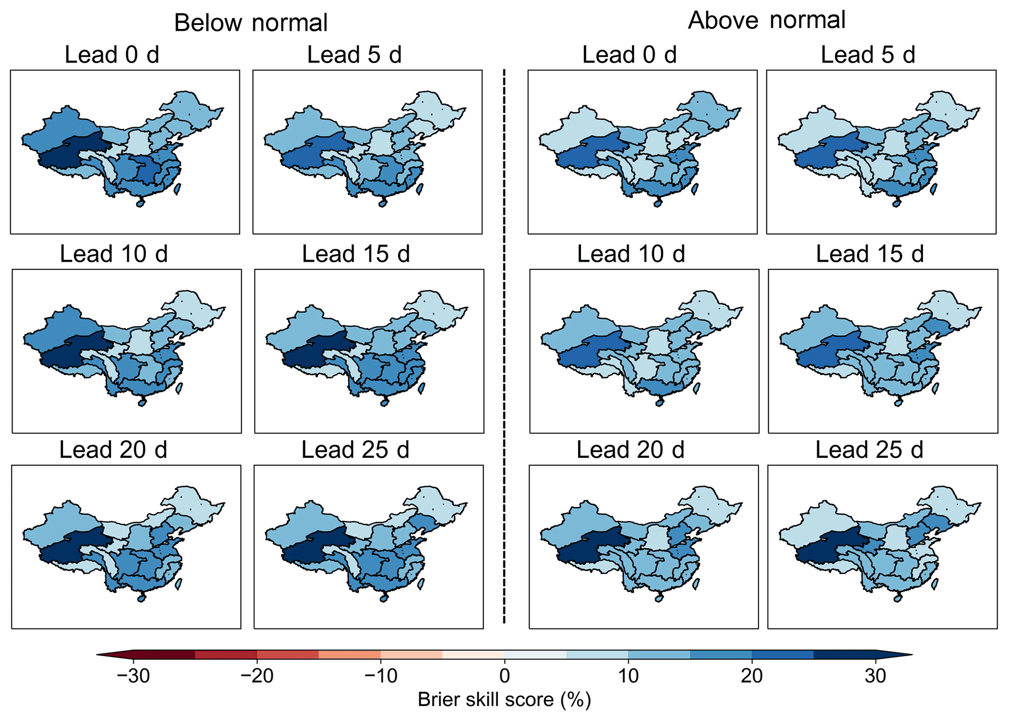
Figure 6 The Brier skill scores of the STP-BHM model for the prediction of below-normal and above-normal events of the pentad mean precipitation amount at different lead times during the period of 1979–2016, from May to October.

To help identify the main sources of subseasonal precipitation predictability, we also establish the STP-BHM model for each atmospheric field separately. Figure 7 compares the CRPS skill scores of the pentad mean precipitation forecasts with different predictors. In general, U850, U200, H850, and H500 show higher forecast skill compared to the OLRAs and H200 for almost all hydroclimatic regions and lead times. This suggests that the ISO signals of these atmospheric fields contribute more to the overall forecast skill. Compared to the STP-BHM model built with only one predictor, the forecast skill is further improved when all ISO signals of atmospheric fields are used.

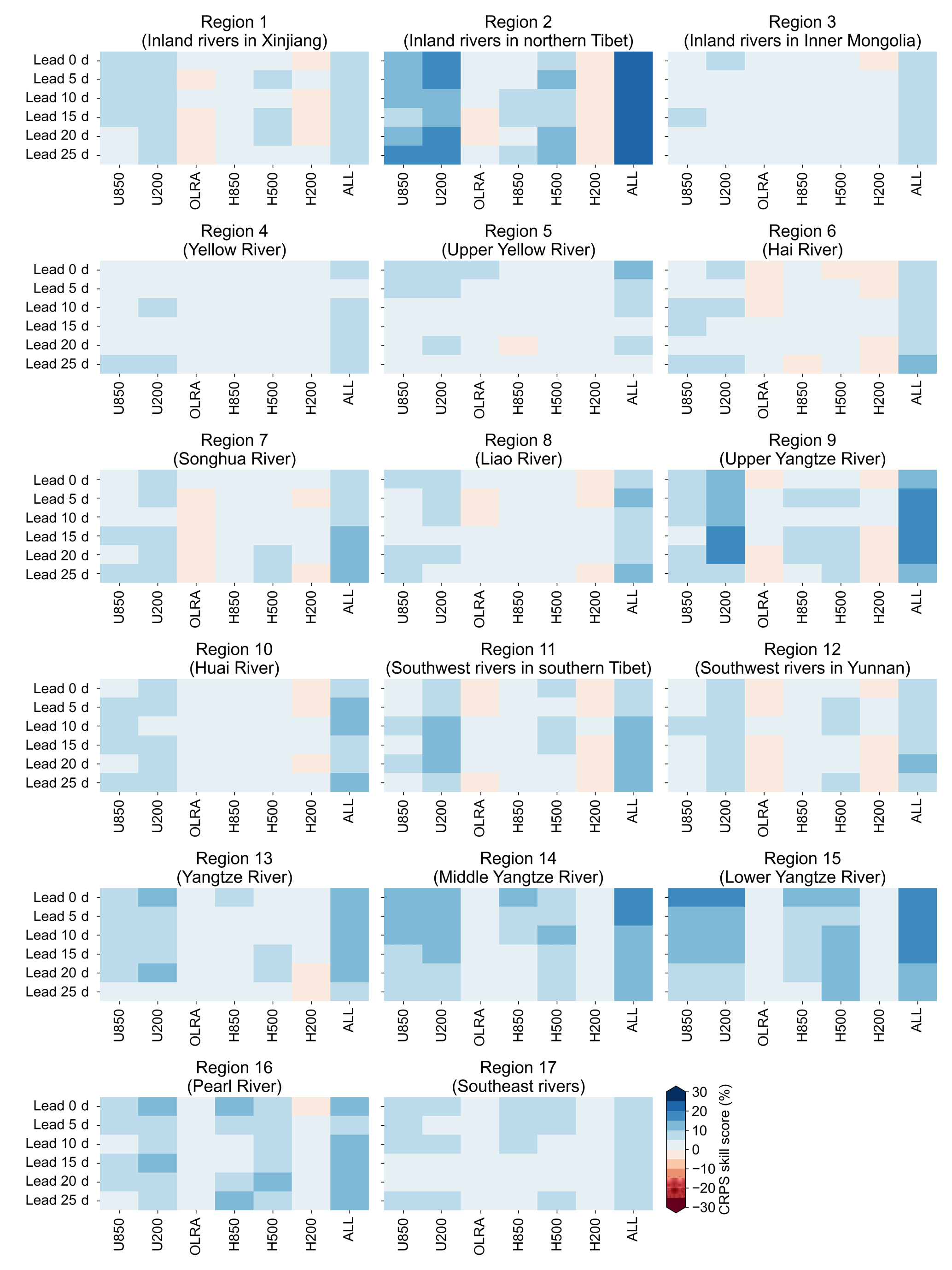
Figure 7 The cross-validated CRPS skill scores of the STP-BHM model for the pentad mean precipitation amount forecasts with different predictors (U850, U200, OLRAs, H850, H500, and H200). The term “ALL” denotes that the ISO signals of all atmospheric fields are used as predictors.

The attribute diagrams of the subseasonal forecasts of the pentad mean precipitation amount for below-normal and above-normal events at different lead times are shown in Fig. 8. Most points fall near the 1:1 line for both below-normal and above-normal events at all lead times. This suggests that the probabilistic forecast distributions are reliable. However, the forecast probabilities deviate slightly from the 1:1 line at higher forecast probabilities for above-normal events, indicating that the sharpness for above-normal events should be further improved.

Figure 8 The attribute diagram of the STP-BHM model for the prediction of below-normal and above-normal events of the pentad mean precipitation amount at different lead times. The forecast probability is binned with a width of 0.2. The size of each dot represents the fraction of forecasts that falls into a particular probability bin.

Figure 9 compares the CRPS skill scores of the STP-BHM model and the NCEP model from May to October during the period of 1999–2010. It is not surprising that the NCEP model outperforms the STP-BHM model when the lead time is within 5 d. However, we should note that the STP-BHM model shows a much higher probabilistic forecast skill compared to the NCEP model at longer lead times. Positive CRPS skill scores are observed for the STP-BHM model over most hydroclimatic regions, whereas the skill scores are mostly negative for the NCEP model.

Figure 9 Comparison of the CRPS skill scores of the STP-BHM model and the NCEP model during the period of 1999–2010, from May to October.

3.2 Forecast skill of pentad mean precipitation anomalies

The cross-validated CRPS skill scores for the subseasonal forecasts of the pentad mean precipitation anomalies are shown in Fig. 10. The STP-BHM model shows positive CRPS skill scores over most hydroclimatic regions, except inland rivers in Xinjiang (Region 1) and inland rivers in northern Tibet (Region 2). This may be explained by the relatively lower variability in the pentad mean precipitation anomalies in these regions. In addition, the STP-BHM model shows higher forecast skill in eastern China, with CRPS skill scores ranging from 10 % to 15 %. In comparison, the forecast skill in inland rivers in Inner Mongolia (Region 3), the upper Yellow River (Region 5), the upper Yangtze River (Region 9), the southwestern rivers in southern Tibet (Region 11), the southwestern rivers in Yunnan (Region 12), the Yangtze River (Region 13), and the Pearl River (Region 16) are lower. Similar results are also found by Zhu and Li (2017c), for which southwestern China shows a lowest forecast skill compared to other regions.

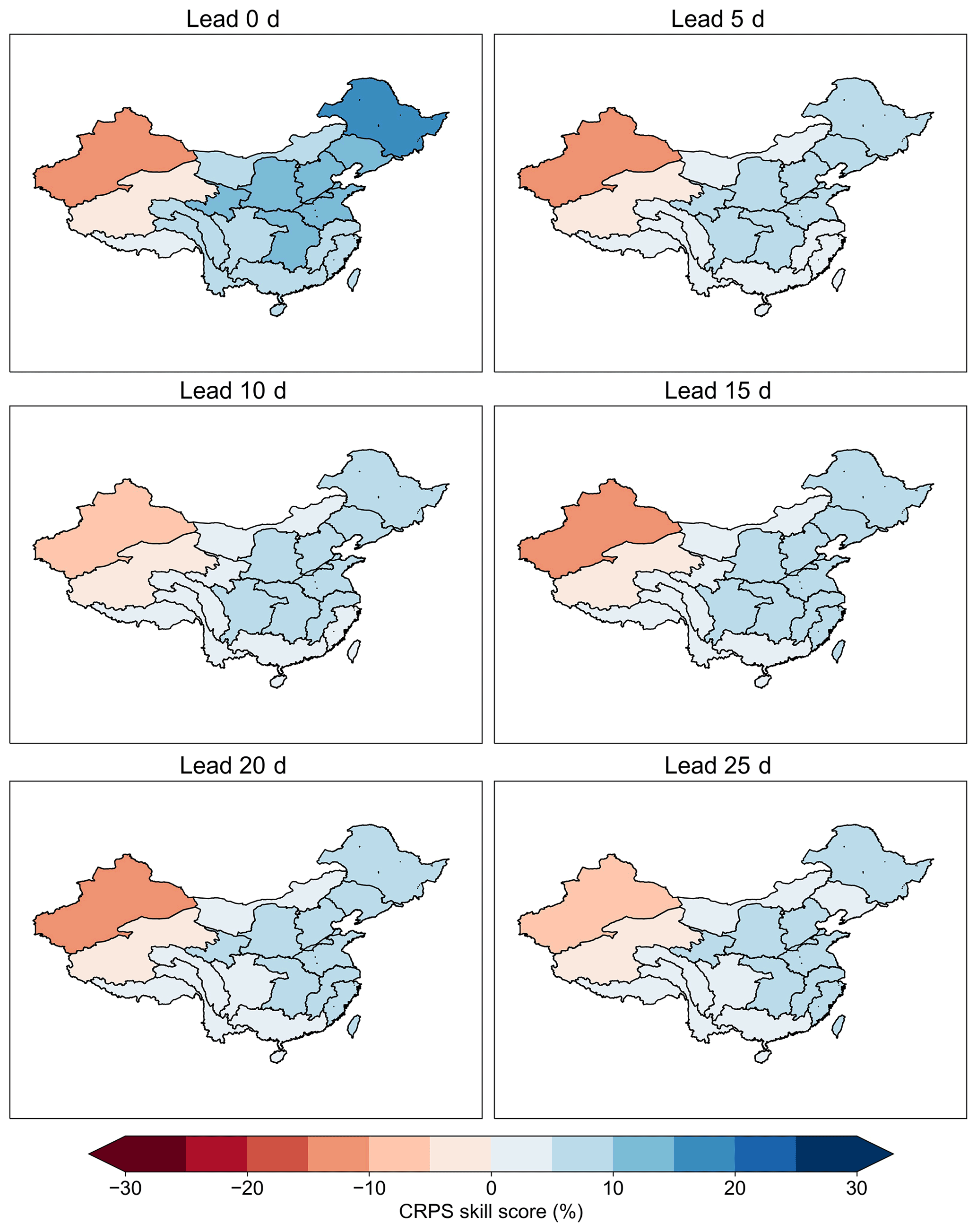
Figure 10 Same as Fig. 5 but for pentad mean precipitation anomalies.

The Brier skill scores of the pentad mean precipitation anomalies for below-normal and above-normal events are presented in Fig. S33. Positive Brier skill scores are found over all regions and all lead times, indicating that the STP-BHM model outperforms the cross-validated climatological forecasts for extreme events. Meanwhile, the differences in the Brier skill scores in different hydroclimatic regions are small, where the Brier skill scores are mostly ranging from 5 % to 15 % for both below-normal and above-normal events.

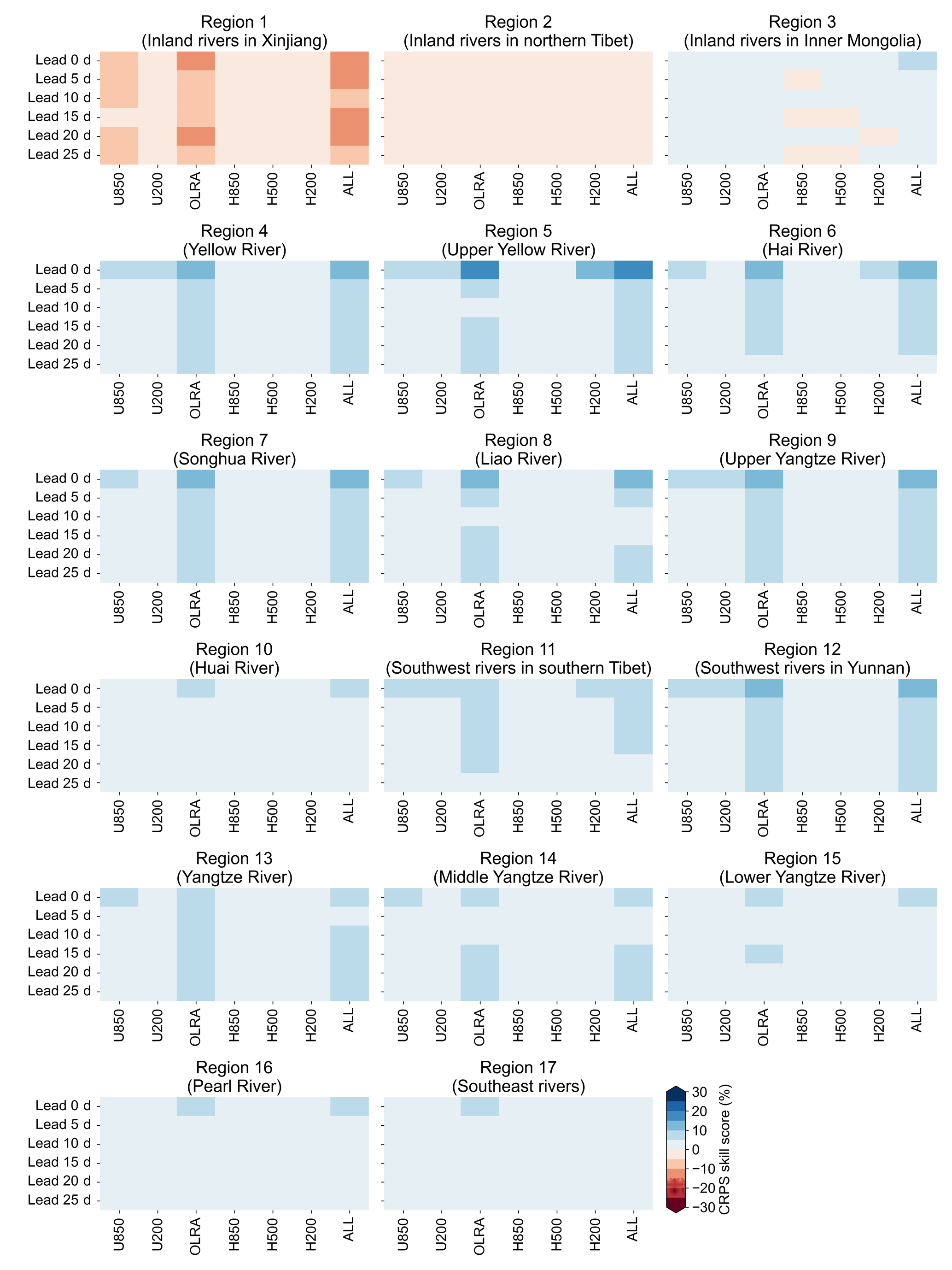
Figure 11 compares the CRPS skill scores of pentad mean precipitation anomalies with different predictors. Overall, the STP-BHM model with OLRAs used as predictors shows higher forecast skill compared to other predictors for almost all hydroclimatic regions and lead times. This suggests that the OLRAs contribute most to the overall forecast skill of the pentad mean precipitation anomalies.

Figure 11 Same as Fig. 7 but for pentad mean precipitation anomalies.

Shown in Fig. S34 is the attribute diagram of the subseasonal forecasts of the pentad mean precipitation anomalies for below-normal and above-normal events at different lead times. Most points fall close to the 1:1 line for both below-normal and above-normal events. This suggests that the probabilistic forecast distributions are reliable for the pentad mean precipitation anomalies as well. The sharpness of STP-BHM model is also observed, especially for below-normal events.

4 Discussion

4.1 Forecast skill and possible mechanism

In this study, we first analyze the relationship between the preceding ISO signals of the atmospheric fields and precipitation. The coupled patterns are extracted, and the corresponding projection coefficients are defined as predictors. A Bayesian hierarchical model is then established and applied to predict both the pentad mean precipitation amount and the pentad mean precipitation anomalies over China. Our results suggest that the STP-BHM model can provide skillful and reliable probabilistic forecasts for both the pentad mean precipitation amount and the pentad mean precipitation anomalies at a lead of 20–25 d over most hydroclimatic regions in China. However, the spatial patterns of skill scores suggest that the STP-BHM model is more skillful over southern China. This may be explained by the different characteristics of intraseasonal variability and different possible mechanism over different hydroclimatic regions. Wang (2007) analyzed the precipitation variability from April to September over China, and the results suggested that the seasonal component accounted for nearly 70 % of the total variability over northeastern China. The intraseasonal (10–90 d) component only accounted for nearly 7 % of the total variability, which indicates that the intraseasonal precipitation over these regions has no significant frequency peak. In comparison, the subseasonal component accounted for over 20 % of the total variability in southeastern China. Ouyang and Liu (2020) also found that the boreal summer monsoon intraseasonal variability in precipitation over the lower Yangtze River basin was mainly dominated by the relatively low-frequency 12–20 d variability and high-frequency 8–12 d variability. Wang and Duan (2015) demonstrated that the quasi-biweekly oscillation (QBWO; 10–20 d oscillation) was the dominant mode of intraseasonal variability in summer precipitation over the Tibetan Plateau. The relations between atmospheric intraseasonal oscillation and the low-frequency variability in precipitation vary from region to region as well. Ren and Shen (2016) suggested that the impact of the tropical atmospheric intraseasonal oscillation on precipitation was more significant in regions in southern China and the Tibetan Plateau areas during the boreal summer. We also note that the forecast skill of pentad mean precipitation amounts and precipitation anomalies is different. The precipitation amounts vary at different timescales (interannual, intraseasonal, and synoptic). The large-scale circulation anomalies (U850, U200, H850, and H500) may be dominant for the total variability in precipitation amounts. In comparison, the precipitation anomalies only represent the intraseasonal component of precipitation. The OLR plays a more important role for intraseasonal convections compared to other dynamical fields (Ventrice et al., 2013; Liu et al., 2016).

We should also note that the CRPS skill scores of the STP-BHM model are lower than NCEP dynamical models at short lead times. The Calibration, Bridging, and Merging (CBaM) method, which makes the best use of GCM outputs, has been proved to be efficient for improving seasonal precipitation over many regions (Strazzo et al., 2019; Schepen and Wang, 2013; Peng et al., 2014). Recently, Specq and Batté (2020) proposed a similar statistical dynamical approach to improve the subseasonal precipitation forecasts over the southwestern tropical Pacific. In the future, the statistical forecasts generated from lagged atmospheric indices should be included in the calibrated forecasts to further improve the subseasonal precipitation forecast skill.

4.2 Limitations and future work

In this study, the correlation between the ISO signals of atmospheric fields and precipitation is analyzed using the whole record, despite the cross-validation strategy used for statistical modeling. This may introduce artificial skill into the model to some extent. However, the correlation analysis for each step of the cross-validation is difficult in practice. We analyze the spatial patterns of the correlations between the preceding ISO signals of U850 and the precipitation over Region 1 at the lead time of 0 d for the period of 1979–2016 and 1980–2016 (Fig. S35). The results show a small variability between the cross-validated correlation and the whole-period correlation. In addition, the cross-validation strategy used in the statistical modeling procedure can also reduce the chance of overfitting (Vehtari and Lampinen, 2002; Delsole and Shukla, 2009).

Another limitation of this study is the treatment of zero values adopted in the statistical modeling procedure. We treat the zero values as censored data, also referred as the explicit approach in McInerney et al. (2019). Although this treatment performed well in low-ephemeral and mid-ephemeral catchments, the performance of this explicit approach was poor in high-ephemeral (>50 % zero flows) catchments. Further development is required to overcome this problem. The copula functions are flexible in choosing marginal distributions and have been widely used in hydrological simulations in recent years (Zhang and Singh, 2007; Vernieuwe et al., 2015; De Michele and Salvadori, 2003). Compared to the Bayesian statistics we used in this study, the copula functions are more general, and the normalization may not be required when the skewed distributions are used as the marginal distribution of precipitation. This may provide a possible solution to overcome the problems caused by the large number of zero values.

We built the Bayesian hierarchical model for each hydroclimatic region separately. However, the spatial patterns of precipitation have not been considered yet. The spatial Bayesian hierarchical model, which can capture the spatial dependence of precipitation between different regions, could be used to provide subseasonal precipitation forecasts with spatial coherence (Reza Najafi and Moradkhani, 2013; Bracken et al., 2016). An alternative way to reconstruct the spatial patterns of probabilistic precipitation forecasts is to use the Schaake shuffle method or ensemble copula coupling method (Roman et al., 2013; Clark et al., 2004). Higher spatial or temporal resolutions of the precipitation forecasts are also needed for the subseasonal streamflow forecasts. However, our previous studies indicated that post-processed daily precipitation forecasts from GCMs are of low accuracy when the lead time is beyond 10–14 d (Li et al., 2020). In this study, the large-scale ISO signals are only used to predict the pentad mean precipitation, as the noise of daily precipitation is too large. Spatial or temporal disaggregation may be required in the future to provide daily precipitation forecasts as inputs for hydrological models.

5 Conclusions

Accurate and reliable subseasonal precipitation forecasts are difficult, as the predictability from atmospheric initialization is lost after 2 weeks, while the slowly varying boundary conditions do not have a substantial impact at such a timescale. The intraseasonal oscillation (ISO) is considered to be one of the leading sources of subseasonal predictability. However, the relationship between atmospheric intraseasonal signals and precipitation is of high uncertainty. In this study, we first analyze the correlation between the preceding atmospheric intraseasonal signals (U850, U200, OLRAs, H850, H500, and H200) and precipitation. The spatiotemporal coupled covariance patterns are constructed for grid points where the correlation statistically significant at the 5 % level. The predictors are then defined by summing the product of the covariance fields and ISO signals of atmospheric field. A Bayesian hierarchical model (BHM) is then built to address the uncertainty in the relationship between the ISO signals of atmospheric fields and precipitation. The posterior distributions of the model parameters are sampled using a Gibbs sampling algorithm. The STP-BHM model is used to predict both the pentad mean precipitation amount and pentad mean precipitation anomalies after parameter inference. The performance is evaluated through a leave-1-year-out cross-validation strategy.

Our results suggest that the STP-BHM model we built in this study can provide skillful and reliable probabilistic forecasts for both the pentad mean precipitation amount and the pentad mean precipitation anomalies at a lead time of 20–25 d over most hydroclimatic regions in China when all ISO signals of the atmospheric fields are used as predictors. In addition, the STP-BHM model shows useful predictive skill for below-normal and above-normal events as well, and positive Brier skill scores are observed at all lead times. The spatial patterns of the skill scores suggest that the STP-BHM model is more skillful over southern China compared to other regions. The STP-BHM model outperforms the NCEP S2S dynamical model when the lead time is beyond 5 d. To help identify the main sources of the subseasonal precipitation predictability, we also establish the STP-BHM model for U850, U200, OLRAs, H850, H500, and H200 separately. The results suggest that the ISO signals of U850, U200, H850, and H500 contribute more to the overall forecast skills for the pentad mean precipitation amount predictions. In comparison, the OLRAs contribute the most to the forecast skill for predictions of the pentad mean precipitation anomalies.

In this study, the spatial patterns between the ISO signals of the zonal wind at 850 and 200 hPa, outgoing longwave radiation, and the geopotential height at 850, 500, and 200 hPa are extracted and used to define predictors. Other sources of the subseasonal predictability, such as soil moisture, snow cover, and stratosphere–troposphere interaction, will be included in the Bayesian hierarchical model to further improve the subseasonal precipitation forecasts. The Calibration, Bridging, and Merging (CBaM) method can also be investigated at a subseasonal timescale to further improve the forecast skill (Schepen and Wang, 2013; Schepen et al., 2014).