the Creative Commons Attribution 4.0 License.
the Creative Commons Attribution 4.0 License.
 | 29 Sep 2022
Development of a national 7-day ensemble streamflow forecasting service for Australia
Hapu Arachchige Prasantha Hapuarachchi
Mohammed Abdul Bari
Aynul Kabir
Mohammad Mahadi Hasan
Fitsum Markos Woldemeskel
Nilantha Gamage
Patrick Daniel Sunter
Xiaoyong Sophie Zhang
David Ewen Robertson
James Clement Bennett
Paul Martinus Feikema
Reliable streamflow forecasts with associated uncertainty estimates are essential to manage and make better use of Australia's scarce surface water resources. Here we present the development of an operational 7 d ensemble streamflow forecasting service for Australia to meet the growing needs of users, primarily water and river managers, for probabilistic forecasts to support their decision making. We test the modelling methodology for 100 catchments to learn the characteristics of different rainfall forecasts from Numerical Weather Prediction (NWP) models, the effect of statistical processing on streamflow forecasts, the optimal ensemble size, and parameters of a bootstrapping technique for calculating forecast skill. A conceptual rainfall–runoff model, GR4H (hourly), and lag and route channel routing model that are in-built in the Short-term Water Information Forecasting Tools (SWIFT) hydrologic modelling package are used to simulate streamflow from input rainfall and potential evaporation. The statistical catchment hydrologic pre-processor (CHyPP) is used for calibrating rainfall forecasts, and the error reduction and representation in stages (ERRIS) model is used to reduce hydrological errors and quantify hydrological uncertainty. Calibrating raw forecast rainfall with CHyPP is an efficient method to significantly reduce bias and improve reliability for up to 7 lead days. We demonstrate that ERRIS significantly improves forecast skill up to 7 lead days. Forecast skills are highest in temperate perennially flowing rivers, while it is lowest in intermittently flowing rivers. A sensitivity analysis for optimising the number of streamflow ensemble members for the operational service shows that more than 200 members are needed to represent the forecast uncertainty. We show that the bootstrapping block size is sensitive to the forecast skill calculation. A bootstrapping block size of 1 month is recommended to capture maximum possible uncertainty. We present benchmark criteria for accepting forecast locations for the public service. Based on the criteria, 209 forecast locations out of a possible 283 are selected in different hydro-climatic regions across Australia for the public service. The service, which has been operational since 2019, provides daily updates of graphical and tabular products of ensemble streamflow forecasts along with performance information, for up to 7 lead days.
- Article
(3490 KB) - Full-text XML
- BibTeX
- EndNote


Optimal management of water resources requires support from accurate, reliable, and timely streamflow forecasts to make decisions. Practical and scientific benefits of predictive modelling of hydrological processes are evident (Shmueli, 2010) and have long been recognised. Water forecasting models can make significant contributions to drought mitigation and alleviation, optimal management of urban and agricultural water allocations, basin planning, hydropower generation, and flood management and mitigation (Buizer et al., 2016). Skilful streamflow forecasts can significantly contribute to improving reservoir operation, water supply storage reliability, and environmental allocation (Delaney et al., 2020). In the long term, these predictive hydrological models can potentially bring enormous benefits to the environment and society, ensuring economic growth and environmental sustainability (Talukder and Hipel, 2020).
Water and flood managers need accurate streamflow forecast information with a useful lead time to make optimal water management decisions. The useful lead time can be hours to years depending on the type of application and actions required. There is a wide range of modelling techniques, from conceptual, physically-based, statistical, and stochastic time series to modern hybrid artificial intelligence (AI) models that can be used for streamflow forecasting. Conceptual and physically-based models are more commonly used for short- and medium-term streamflow forecasting. Statistical models such as the Bayesian joint probability (BJP) model (Robertson and Wang, 2012; Zhao et al., 2016; Charles et al., 2018) are mostly used for monthly- or seasonal-timescale streamflow forecasting. Recently, machine learning tools based on data pre-processing techniques and swarm intelligence algorithms have been successfully used for short-term streamflow forecasting (Niu et al., 2020). Commonly, rainfall forecasts from a Numerical Weather Prediction (NWP) model are used as input to a calibrated hydrological model for streamflow forecasting. Over the last few decades, NWP has moved from deterministic to probabilistic (ensemble) forecasting. As a result, probabilistic streamflow forecasting has become increasingly popular across the globe (Pappenberger et al., 2016; Wu et al., 2020; Roy et al., 2017). Probabilistic forecasts provide estimates of uncertainty involved in the forecasts that assist users in making informed decisions from the different scenarios available.
There are several large-scale (continental and global) hydrological systems run by communities around the world (Bierkens et al., 2015; Emerton et al., 2016). The Global Flood Awareness System (GloFAS) is one such forecasting system that can skilfully predict extreme events in large river basins up to 1 month ahead (Alfieri et al., 2013). The European Flood Awareness System (EFAS, Smith et al., 2016), operational since 2012, is a European Commission initiative developed by the Joint Research Centre (JRC) for riverine flood preparedness across Europe. The service aims to provide harmonised early warnings and hydrological information to national agencies across Europe. The US hydrologic ensemble forecast service (HEFS), run by the National Weather Services (NWS), provides ensemble streamflow forecasts that seamlessly span lead times from less than 1 h to several years, and that are spatially and temporally consistent for river basins across the US (Demargne et al., 2014). Siddique and Mejia (2017) report that the ensemble streamflow forecasts in the US mid-Atlantic region remain skilful for lead times up to 7 d. Post-processing of the forecasts increased forecast skills across lead times and spatial scales. The past research demonstrates that ensemble streamflow predictions at different temporal scale is possible, but the skills vary from one geographical location to another. These findings give us greater confidence for the development of an operational ensemble streamflow forecasting service for Australia.
Australia is a land of extremes from droughts to floods and raging fires. It has a wide range of geographical and topographical features with a large central arid or semi-arid zone. The southeast and southwest regions are temperate, and the north has a tropical climate (Stern et al., 2000). These unique geographical features result in the most significant inter-annual variability of streamflow, floods, and droughts compared with other continents (Poff et al., 2006). During 2001–2009 south-eastern Australia experienced its most severe drought since 1901, known as the “Millennium Drought” (http://www.bom.gov.au/climate/drought/knowledge-centre/previous-droughts.shtml, last access: 16 September 2022). The region had the most extended period of below-median rainfall and, as a result, inflows to major reservoirs were very low (Van Dijk et al., 2013). In particular, inflow to reservoirs located within the Murray–Darling River basin, Australia's food bowl, was 50 % of the previously recorded minimum. The drought had wide, long-lasting societal, economic, and environmental impacts (Bureau of Meteorology, 2021). As a result, the federal government passed the Water Act 2007 (https://www.legislation.gov.au/Details/C2017C00151, last access: 16 September 2022) to implement a water security plan for the nation. One of the critical components of implementing the water security plan was developing and operationalising streamflow forecasting services at different temporal scales with special emphasis on short-term (hours to days) and medium-term (months to seasons) forecasts. The Bureau of Meteorology (BoM) launched a seasonal streamflow forecasting service (Woldemeskel et al., 2018; Feikema et al., 2018) in 2010 (http://www.bom.gov.au/water/ssf/history.shtml, last access: 16 September 2022). A 7 d deterministic streamflow forecasting service (Hapuarachchi et al., 2016) was progressively developed during 2010–2017 and released to the public. More recently, stakeholders showed greater interest in probabilistic streamflow forecasts as it provides information on the uncertainty involved in the forecasts and supports users in making informed decisions with associated uncertainties. In response, the BoM launched the 7 d ensemble streamflow forecasting (SDF) service (http://www.bom.gov.au/water/7daystreamflow/, last access: 16 September 2022) in December 2019, upgrading the existing deterministic service. The upgraded service provides a set of forecasts to give an indication of a range of possible streamflow outcomes based on input forecast rainfall uncertainties for up to 7 d lead time at an hourly scale at different river gauge stations with useful skill and reliability.
This paper describes the development of a SDF service, including the characteristics of different Numerical Weather Prediction (NWP) model rainfall forecasts, application of calibration to forecast rainfall, error modelling of streamflow forecasts, the optimal ensemble size required to represent the forecast uncertainty, parameters of a bootstrapping technique for calculating forecast skill, operational implementation of the service, and future work. The next sections of the paper describe the methodology, verification metrics, catchments and data, results, discussion, and future work.
The adopted hybrid dynamical–statistical streamflow forecasting method consists of several components. It includes NWP calibration, hydrological modelling and hydrological error modelling, and we firstly introduce the components of the system. The forecasting system is premised on separating rainfall forecasting from hydrological modelling. This includes separating the estimation of uncertainty in rainfall forecasts from the estimation of uncertainty in hydrological models. The system is thus a hybrid dynamical–statistical forecasting system. This setup has several key benefits: it makes the system highly modular, allowing new models (e.g. new NWPs) to be substituted into the system without the need to revise other components (e.g. the hydrological model). Second, it means that more appropriate techniques can be applied to estimate forecast uncertainty in each case: for example, error models are better able to handle the strong autocorrelation in streamflow than statistical calibration methods typically applied to rainfall forecasts. There are only a few streamflow forecast systems around the world using this hybrid technology. The hydrologic ensemble forecast system (HEFS, Demargne et al., 2014) is a hybrid forecast system. It applies a calibration to rainfall and an error model. However, in an operational setting, it uses “in-the-loop” flood forecasters to manually do data assimilation, which may impede the ability to produce reliable ensemble forecasts. The European Flood Awareness System (EFAS) and Global Flood Awareness System (GloFAS) use dynamical models only.
Operationalisation of the system requires many practical scientific questions to be addressed. In this paper we seek to identify:
- a.
the minimum ensemble size that can be used while maintaining robust performance
- b.
how best to describe forecast skill when only limited hindcast dataset is available.
Our methods then describe the approach taken to answer these questions. A verification strategy is critical to answer the operationalisation questions and provide an assessment of the forecast performance. We finally describe the verification strategy adopted for this study.
2.1 Calibration and evaluation of rainfall forecasts
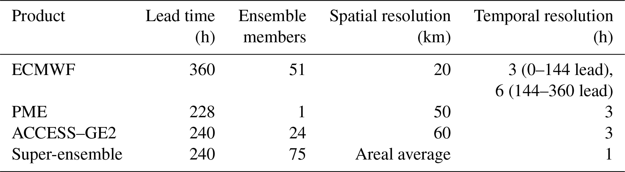
Three NWP rainfall forecast products (Table 1) are evaluated for 100 catchments (at the outlets) in this study to understand their characteristics and to explore the impact of calibration. These are the European Centre for Medium-Range Weather Forecasts (ECMWF) atmospheric model ensemble forecasts (Richardson, 2000), Australian Community Climate and Earth-System Simulator–global ensemble (ACCESS–GE2) forecasts (O'Kane et al., 2008), and the BoM's poor man's ensemble (PME) (Ebert, 2001), the ensemble mean of NWP models from Australia, UK, USA, Canada, Europe, and Japan. Note that ACCESS-GE2 was a pre-operational product made available for this study, and a newer version (ACCESS–GE3) is now available. A catchment is delineated to sub-catchments and finer sub-areas using a national flow direction map to represent a semi-distributed model structure. A hydrological model is applied to each sub-area with average areal rainfall (see Sect. 2.2.1). The average areal rainfall of each sub-area per each ensemble member is calculated by taking the area-weighted average of gridded forecast rainfall for all grid cells intersecting the sub-area. The average forecast rainfall is post-processed using the catchment hydrologic pre-processor (CHyPP) model (Robertson et al., 2013), which is based on a Bayesian joint probability (BJP) model that defines a spatially variable probabilistic relationship between NWP model forecast rainfall and observed rainfall. The BJP model relates forecast rainfall to corresponding observations using a log-sinh transformed bivariate normal distribution. The log-sinh transformation is applied to normalise observed and forecast rainfall data and to homogenise their variance. The Schaake shuffle (Clark et al., 2004) method used in the CHyPP generates spatially and temporally coherent calibrated forecasts by linking samples from forecast probability distributions at each consecutive lead time within the entire hindcast period for each forecast location within the catchment.
A leave-one-month-out cross-validation procedure (Hapuarachchi et al., 2016) is applied to calibrate and validate the CHyPP model for the data period of 36 months from 2014 to 2016. ACCESS–GE2 hindcast data are limited and 2014–2016 is the common period of data available for the selected NWP rainfall products. Given that PME is a merged post-processed product of many global NWP products, it shows negligible improvement when CHyPP is used on it (Shrestha et al., 2020). Therefore, the PME forecasts are not post-processed. We also call a raw super-ensemble, a merged product of ECMWF, ACCESS–GE2, and PME with 75 members (Table 1). The 3 and 6 h NWP data (Table 1) are disaggregated to hourly using linear interpolation within CHyPP. Bennett et al. (2016) showed that even converting daily rainfall totals to hourly using linear interpolation produces plausible rainfall–runoff model outputs. By calibrating the forecasts with CHyPP, we generate x number of bias-corrected statistically reliable ensemble members for each rainfall forecast product, ACCESS–GE2 and ECMWF, and merge them with PME (total OES members) that is referred to as a post-processed super-ensemble. The x to be determined is based on the analysis on optimum ensemble size (present below). Raw and post-processed rainfall forecasts are evaluated independently (Table 2) for different lead times at the catchment scale for bias, precision, and reliability (see Sect. 2.5 for details). Note that PME is included here mainly for generating a deterministic streamflow forecast to embed in the ensemble plume of the forecast products of the operational service.
2.2 Generating and evaluating streamflow forecasts
2.2.1 Rainfall–runoff model and channel routing
The core hydrologic modelling package used here is the Short-term Water Information Forecasting Tools (SWIFT) (Perraud et al., 2015). SWIFT consists of many hydrologic modelling tools including conceptual hydrologic models, catchment routing models, channel routing models, streamflow error models, and parameter optimisation methods. It supports deterministic and ensemble hydrologic modelling for the retrospective evaluation of catchment models using hindcast data and real-time forecasting. Previous research conducted in Australia (Perrin et al., 2003; Coron et al., 2012; Van Esse et al., 2013; Bennett et al., 2016; Kunnath-Poovakka and Eldho, 2019) and elsewhere have shown that GR4J (Perrin et al., 2003) and its variants perform at least as well as other conceptual models in a range of environments at daily and hourly time-steps. Therefore, the GR4H rainfall–runoff model (Bennett et al., 2014), an hourly variant of the daily GR4J model and lag and route channel routing is implemented here.
A nationally consistent flow direction map from the Australian Hydrological Geospatial Fabric (Geofabric) (Atkinson et al., 2008) is used to delineate each catchment into sub-catchments which is then further divided into finer sub-areas based on the flow direction, the coverage of gauging stations, and hydro-climatic characteristics such as the rainfall gradient. It therefore represents a semi-distributed model structure. A collection of upstream sub-areas makes a sub-catchment where a streamflow gauge exists at the outlet. For the 100 catchments, the size of a sub-area varies from 30 to 4000 km2, of which the mean and median values are 600 and 450 km2, respectively. Larger sub-areas are present where the rainfall gradient is insignificant, and rainfall and water level gauge networks are sparse. The hydrologic model is applied to each sub-area. The model is calibrated for each sub-catchment where all the sub-areas within a sub-catchment have the same parameters. However, sub-areas within a sub-catchment have different precipitation and potential evapotranspiration. As a result, state variables and runoff in each sub-area are different from others. Runoff generated in each sub-area is routed to the catchment outlet using the lag and route method. The model parameters are calibrated using the Shuffle Complex Evolution–University of Arizona (SCE–UA) algorithm (Duan et al., 1994) within the SWIFT package.
2.2.2 Hydrological error modelling
In addition to errors contributing to streamflow forecasts from observed and forecast rainfall (see Sect. 3.2), there are errors in both hydrological model structure and in calibrated model parameters. For an operational forecasting service, it is essential to reduce the forecast uncertainty due to these errors as much as possible to provide highly reliable and accurate forecasts to users. Using the Error Representation And Reduction In Stages (ERRIS) (Bennett et al., 2021; Li et al., 2021) method, we explore the impact of error modelling on streamflow forecasts. ERRIS is applied to address different statistical properties of the forecast error in four stages: (i) hydrological model forecast and data normalisation, (ii) non-linear bias correction, (iii) restricted autoregressive (AR) model updating, and (iv) adjustment of residual distribution. After the hydrologic model and routing model parameters are calibrated, the ERRIS parameters are calibrated for each sub-catchment from upstream to downstream. In simulation mode, observed discharge is passed downstream at each sub-catchment outlet. If the observed discharge is missing, post-processed streamflow is used instead of observed. In forecast mode, post-processed streamflow is passed downstream. Note that ERRIS accounts only for uncertainty from the hydrological modelling component of the system, and not uncertainties in rainfall forecasts. For the streamflow forecasts to be reliable overall, uncertainty from ERRIS must sum to the uncertainty from rainfall forecasts.
2.2.3 Cross-validation and forecast verification
A leave-two-year-out cross-validation approach (Hapuarachchi et al., 2016) is implemented for all catchment models using observed hourly data from 2007 to 2016. The first year of the leave-out period in each iteration is used for model validation. The purpose of the second year is to avoid propagating any hydrological effects from the validation period into the model calibration to make it independent (Hapuarachchi et al., 2016). A longer leave-out period is preferred, but this would shorten the available data for model calibration. The duration of 2 yr is determined as appropriate after considering the limited data available. This approach is applied to all catchment models (Fig. 1a). Once a model is validated, we use the whole dataset to calibrate the model to obtain the final parameter set for each sub-catchment. Raw and post-processed streamflow forecasts are generated using the post-processed super-ensemble rainfall forecasts (Table 2) for the 36 months from 2014 to 2016 (Fig. 1b). Streamflow forecasts before and after error modelling are independently evaluated for different lead times at the outlets of the selected 100 catchments for bias, accuracy, and reliability, as described in Sect. 2.5.
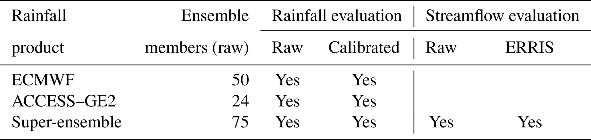
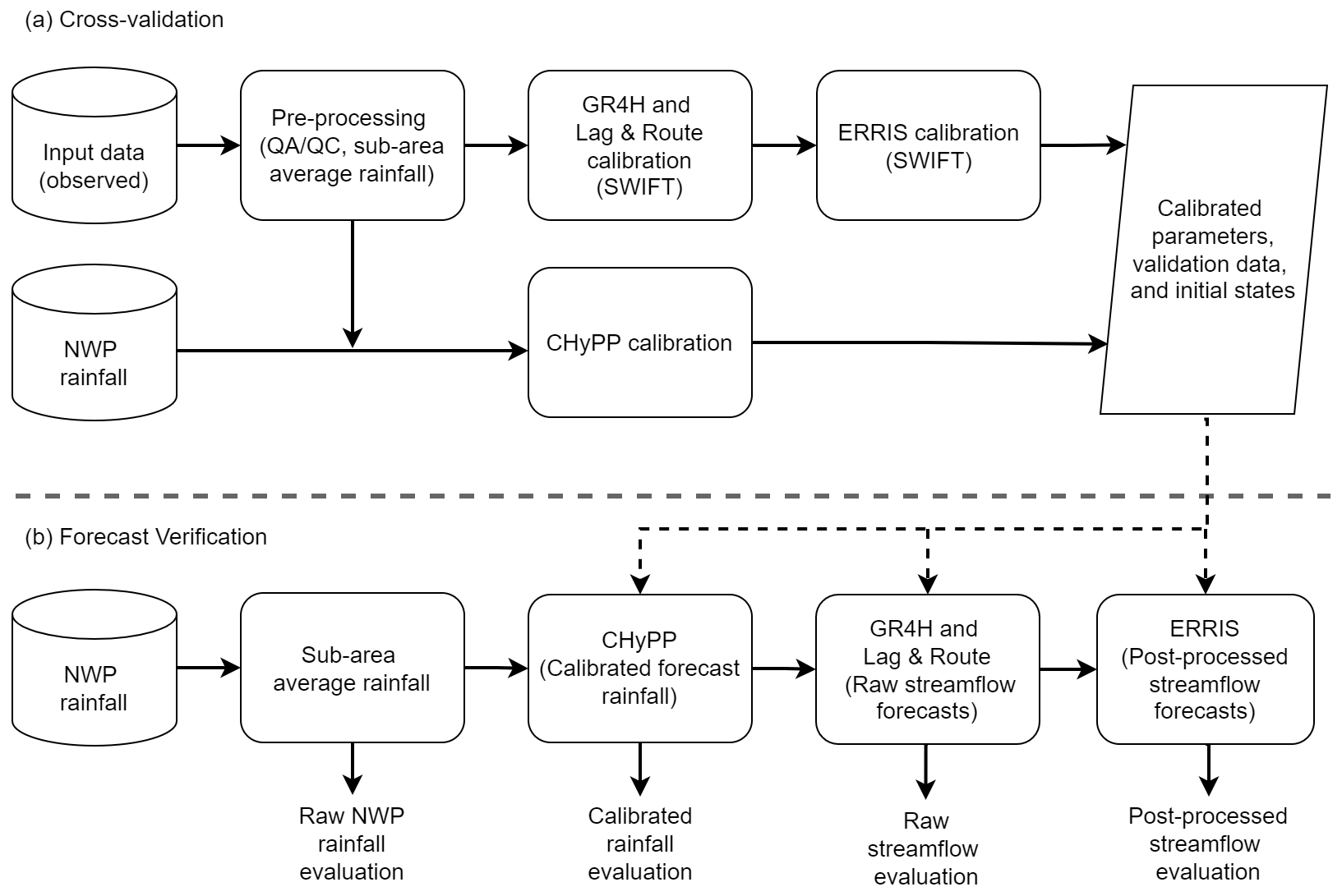
Figure 1Rainfall and streamflow forecast evaluation framework: (a) cross-validation and (b) forecast verification.
2.3 Determination of optimal ensemble size
It is essential to optimise computational efficiency and storage requirements of an operational system without compromising forecast quality. We conduct a sensitivity analysis using six catchments, located in different hydroclimatic regions, to estimate the smallest ensemble size that does not significantly reduce critical measures of forecast performance. We set the maximum ensemble size to 1000 members based on the operational computational capacity. ACCESS–GE2 and ECMWF are calibrated to generate 1000 forecast rainfall members for each product using the hindcast data from 2014 to 2016 (1096 d). Then we generate a 1000-member error-corrected (ERRIS) streamflow forecast from the rainfall hindcast. We randomly select m (>1000) ensemble members from the 1000-member streamflow ensemble dataset (without removing ensemble members) and repeat the process 100 times. In this exercise, m is 50, 100, 200, 300, and 500. Alternatively, different number of ensemble member (m) samples can be generated independently and analysed. However, this would require extensive computational resources that were unavailable to us. Another method is to dress the ensembles (Pagano et al., 2013) to create more members for each forecast time. However, we want to ensure that the forecasts are true ensembles – i.e. each ensemble member can be summed across time to produce reliable forecasts of accumulations (e.g. 7 d streamflow totals). “Ensemble dressing” methods (Pagano et al., 2013; Verkade et al., 2017) that simply add noise to a given lead time are not suitable for this type of calculation. We calculate the continuous ranked probability score (CRPS, see Sect. 2.5) for the randomly selected samples and compare them with the CRPS of the original 1000-member sample. The optimal ensemble size is decided considering the computational efficiency and the statistical characteristics of the randomly selected samples compared to the original 1000-member sample.
2.4 Streamflow forecast quality assessment
Skill score (see Sect. 2.5.3) is a measure of expected forecast skill for a particular forecast location over a specified period. The CRPS is the metric used in this study. Streamflow forecast skill is calculated using a bootstrapping technique (Efron and Tibshirani, 1994) to obtain fair and reliable skill statistics. The bootstrapping is implemented to provide an understanding of the possible range of skills that might be realised over a long period of record when only a short record of hindcasts is available. We also calculate the reliability for verifying forecast quality. A sensitivity analysis is conducted as described below to (i) select the optimum block size used in the bootstrapping method; and (ii) check the effect of the number of bootstrapping iterations on forecast skill. The steps taken are:
-
ACCESS–GE2 and ECMWF are calibrated to generate x forecast rainfall ensemble members of each product using the hindcast data from 2014 to 2016 (1096 d). For each day, there is an hourly rainfall forecast to 7 d lead-time.
-
Calibrated ACCESS–GE2, ECMWF, and raw PME forecast ensembles are merged to generate an OES-member super-ensemble.
-
From the rainfall super-ensemble in (2), generate OES members of hourly streamflow forecasts. This dataset has the dimension of OES × 24 lt × d data points where lt = 7 is lead time (days) and d = 1096 (days).
-
Since we calculate the forecast skill per lead days, the hourly streamflow data are aggregated to daily values. CRPS per day is calculated using the OES ensemble members to generate a matrix MC with the dimension of lt × d CRPS values.
-
Data in MC per lead days are bootstrapped to calculate forecast skill. We randomly and iteratively select a block of data from the MC for each lead days p times such that the total data points are equal to d and calculate the continuous ranked probability skill score (CRPSS, see Sect. 2.5). For an initial investigation, block sizes explored in this study are a week and a month. From now on, we refer to the block sizes w-block for a week and m-block for a month. For example, if the block size is a month, then p is 36 (i.e. 1096/average no. days per month).
-
Repeat step (4) for k times where k is 100, 200, 500, and 1000.
We do not select a block size of 1 d as the high autocorrelation of daily samples means they are not sufficiently independent.
2.5 Verification metrics
2.5.1 Bias
It is important to assess model bias to ensure the model is not consistently underestimating or overestimating streamflow. Bias (Bias) can be positive (underestimation) or negative (overestimation), and is calculated for each lead time using
where G is observed value (rainfall or streamflow), S is simulated/forecast (median of the ensemble) value, and n is total number of observations.
2.5.2 Nash–Sutcliffe efficiency (NSE)
The Nash–Sutcliffe efficiency (NSE) quantifies the relative magnitude of residual variance compared to the measured data variance by
where is mean observed streamflow. In this study, NSE is used to assess the quality of GR4H streamflow simulations (deterministic), not forecasts.
2.5.3 Continuous ranked probability skill score (CRPSS)
Continuous ranked probability score (CRPS) measures the error of all ensemble members with respect to observations by integrating the squared distance between forecast and observed cumulative distribution functions (Hersbach, 2000), and is given by
where F is the cumulative distribution function (CDF), is the forecast probability CDF for the tth forecast case, is the observed probability CDF (Heaviside function), and T is the number of forecasts. Smaller CRPS values are better, and CRPS tends to increase with increased (positive or negative) forecast bias. For a deterministic forecast, the CRPS is replaced with the mean absolute error (MAE), which is the limiting value of CRPS when forecast spread tends to zero. The relative CRPS is represented as percentage of daily observations. Relative CRPS standardises errors to allow easy comparison between catchments.
Skill is a measure of relative improvement of the forecast over a reference forecast. The continuous ranked probability skill score (CRPSS) is given by
where CRPSreference is the reference forecast. For this study, we use climatology as the reference forecast. Data from 1990 to 2016 are used for climatological streamflow calculation. For any given day of the year, the climatology value is the median of the period from 2 weeks before that day to 2 weeks after (i.e. 29 d) over the climatology period excluding the forecast year.
2.5.4 Probability integral transform (PIT) uniform probability plots
We use the probability integral transform uniform probability (PIT) diagram to assess the reliability of ensemble forecasts (Laio and Tamea, 2007). PIT is uniformly distributed for reliable forecasts. It is the CDF of the forecasts Ft(ft) evaluated at observations Gt and is given by
The empirical CDF of the PIT values falls on the 1:1 line when the forecasts are perfectly reliable. Deviation from the 1:1 line indicates a less reliable forecast. To summarise and compare PIT values for many catchments, we use PIT-alpha (Renard et al., 2010) according to
where PIT is the sorted PITt. An α value of 0 indicates the lowest reliability and 1 indicates perfect reliability. As the minimum rainfall amount measurable by tipping bucket rain gauges is 0.2 mm, we have set rainfall values less than 0.2 mm as censored data for PIT calculation.
3.1 Catchment selection
Australia has several climate zones as defined by Köppen Climate Classification (Stern et al., 2000), including equatorial, tropical, and subtropical regions in the north, and temperate regions in the south. The vast interior regions are covered by grassland and desert. There are 13 drainage divisions (Fig. 2), and mean annual rainfall (Fig. 13) for these divisions varies from 276 to 2816 mm (Table 3) calculated using data for the period from 1990 to 2016. Annual average potential evaporation (PE) is generally higher than annual average rainfall in most areas. Therefore, streamflow generation processes are mainly controlled by water-limited environments (Milly et al., 2005) except for the Tasmania division. The pattern of rainfall–runoff and PE distribution within a year across different drainage divisions vary significantly. In the southern part of Australia, the wet season begins in June–July and ends in December–January, while in the northern part of Australia, the wet season starts in November–December and ends in March–April (Bureau of Meteorology, 2021).
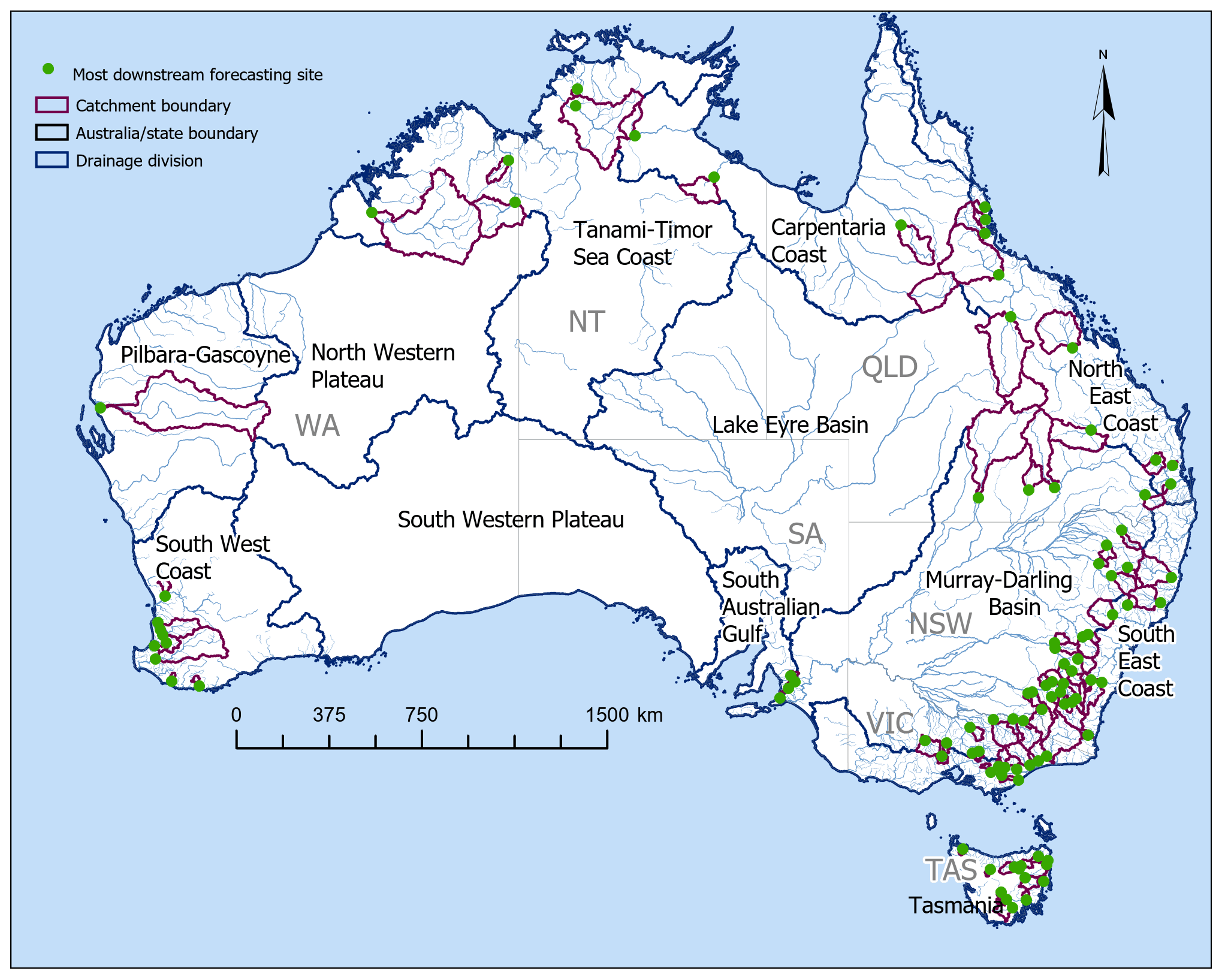
Figure 2Map of Australia showing forecast locations, catchment boundaries, and drainage divisions.
For development of the SDF service, we select 100 catchments in consultation with the state and federal government entities, and water management agencies in different jurisdictions, and consider their strategic value (high economic, environmental, and social significance), data availability, and other factors that support developing a useful model. Most catchments are in the coastal regions (Fig. 2), covering most of Australia's populated centres. For the operational service, 283 potential forecast locations are identified within the selected catchments. There are no forecast locations selected in the South-western Plateau, Lake Eyre, and North-western Plateau divisions (Fig. 2), because there is no significant user demand, and the gauging network is very sparse. Testing and verification of the modelling methodology is done for the outlets of the selected 100 catchments. The same methodology is implemented for modelling all forecast locations within a given catchment.
Table 3Drainage divisions (see Fig. 2) and catchment attributes.
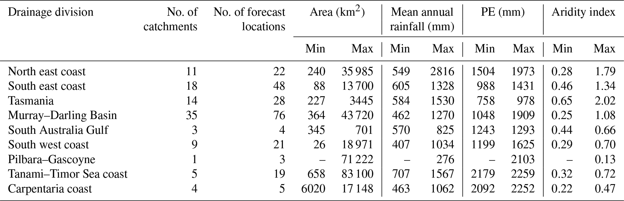
Note: statistics are calculated for the period from 1990 to 2016 using data from all forecast locations in the operational service. Catchment mean annual rainfall is calculated using the hourly rainfall at sub-area centroids computed by interpolating the rainfall of the nearest four gauges. Min and max rainfall and PE, and the aridity index, are calculated from the mean values of rainfall and PE of the catchments within a drainage division. The Pilbara–Gascoyne division has only one catchment, thus min = max. Three drainage divisions with no forecast locations are not included in the table.
3.2 Observed data
This study collates relevant historical observations for consistent retrospective analyses across all catchments from the BoM's databases. Hourly observed streamflow (1990 to 2016) and rainfall data (2007 to 2016) are extracted from the BoM's internal databases and external data provided by water agencies. Due to the limited availability of hourly rainfall data before 2007, the daily rainfall data are extracted from the Australian Water Availability Project (AWAP, Raupach et al., 2009) and disaggregated to hourly time-steps by linear interpolation. The disaggregated hourly rainfall data (from 1990 to 2006) are used for hydrological model warm-up since the quality of disaggregated rainfall data is low at the hourly scale. It is shown that disaggregated daily rainfalls can provide good estimates of states in hourly hydrological models (Bennett et al., 2016). The rainfall and streamflow observations go through a comprehensive quality checking using a semi-automated workflow by visualising streamflow and nearby rainfall station data side by side. This allows the modeller to identify the connection between rainfall and streamflow (i.e. there should be a high rainfall event for high discharge). This approach assists the modeller to confidently make necessary corrections to the observed data. Rainfall data are checked for extreme values, by comparing with data from different sources, and then removing any suspicious values. Streamflow is further checked for rating issues, the rate of change, and continuous zero values because in some locations, missing values are replaced with zeros. Then the quality checked data are visually checked (plots) for further quality assurance. The corrections/modifications made to the original data are recorded (a data file) for future reference by other users of the dataset.
The average areal observed rainfall for each sub-area is calculated using the inverse distance squared weighted averaging method, where the distance is calculated between the rainfall gauge and the sub-area centroid. Monthly gridded PE data (1990 to 2016) at each sub-area centroid are extracted from the AWAP. PE is first disaggregated to daily values by assuming that monthly mean PE occurs in the middle day of each month, then linearly interpolating between these mid-monthly values. Note that this PE disaggregation method ignores the patterns of diurnal cycle and any correlation (negative) with rainfall. However, we note that the method is adequate for this study as Andréassian (2004) showed that GR4J is less sensitive to changes in PE inputs. To generate streamflow forecasts, we use climatological averages of PE calculated over the period 1990 to 2016.
We cross-validate parameters for GR4H, channel routing, and ERRIS for each of the 100 catchment models. In the model validation, 97 of 100 forecast locations exceed the NSE value of 0.6. Catchments with NSE values lower than 0.6 contain intermittent or ephemeral rivers (Table 4). This may be partially due to the lack of representation of nonlinear dynamics in the ephemeral catchment hydrologic processes, including the interaction between groundwater and stream channel, in the GR4H conceptual model. Below, we present detailed results of the experiments (Table 2) to identify the optimal ensemble size, effects of statistical processing, optimal parameters for the bootstrapping method, and acceptance criteria for selecting forecast locations for the operational service.
4.1 Optimal ensemble size
The number of ensemble members required to maintain an acceptable forecast skill (see acceptance criteria in Sect. 4.5) is important for an operational service as the service will generate a large volume of data through daily updates for 100 catchments. Optimal ensemble size is a balance between preserving the statistical properties while not creating unduly large data volumes. We implement the methodology described in Sect. 2.3 to find the optimal ensemble size. The results are consistent across all the selected catchments, so for simplicity, we present results for one catchment. Figure 3 shows the sensitivity of ensemble size on streamflow forecast accuracy (CRPS) with reference to a 1000-member sample for the Tully Catchment (Queensland – QLD). Streamflow forecasts using the ACCESS–GE2 and ECMWF products show similar accuracy for the same sample size (Fig. 3a and b). Generally, the forecast accuracy is proportional to the ensemble size. However, the relative increment of forecast accuracy is inversely proportional to the ensemble size. The overall results indicate that having more than 200 members can preserve greater than 98 % statistical properties of simulated streamflow time series. Noting that multi-model rainfall forecasts provide complementary benefits, and improve the streamflow forecast quality and the robustness of the operational forecast system when the reporting of an NWP product is delayed or unavailable, we recommend using 200 calibrated members (x=200, Sect. 2.4) of each rainfall forecast product (ACCESS–GE2 and ECMWF), for generating streamflow forecasts for the operational service. Merging calibrated ACCESS–GE2 and ECMWF products will not negatively impact on the forecast accuracy (see Sect. 4.3) since they show similar forecast accuracy for the same sample size. The recommendation of 200 calibrated ensemble members from each of the two rainfall forecast products is drawn considering the results shown in Fig. 3, particularly to meet the operational computational efficiency and resources availability at the BoM. In the rest of the paper, we use calibrated ACCESS–GE2 and ECMWF, and raw PME merged product called super-ensemble (OES = 401 members), for streamflow forecast evaluation. The streamflow forecast skill of the super-ensemble is present in Sect. 4.3.
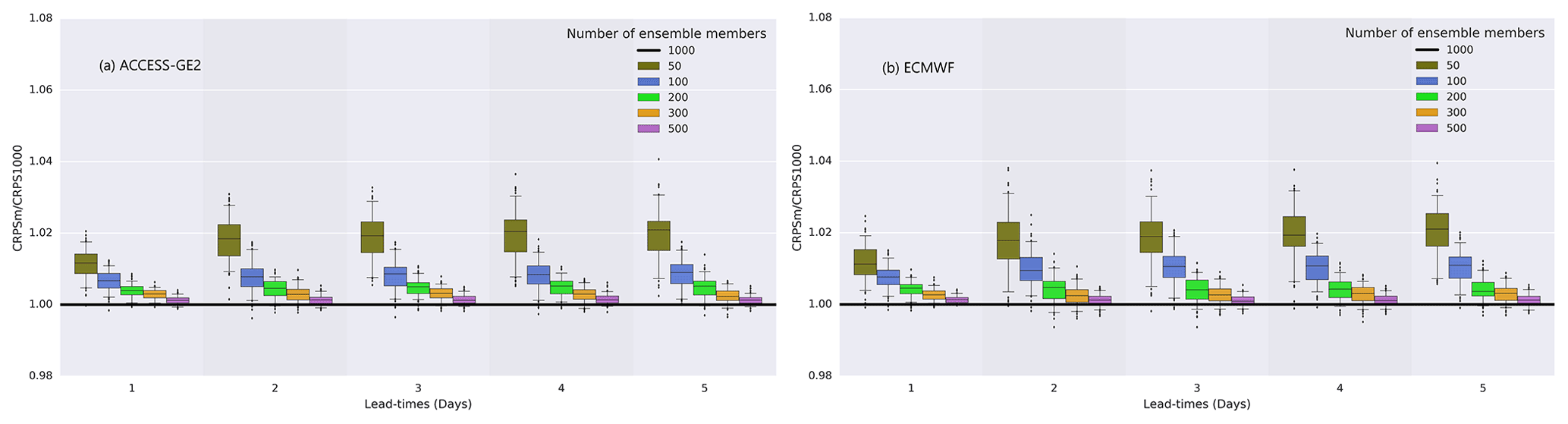
Figure 3Sensitivity of ensemble size to forecast accuracy with reference to a 1000-member sample for rainfall forecasts (a) ACCESS–GE2 and (b) ECMWF for the Tully River at Euramo site (QLD).
4.2 Effect of rainfall calibration
Results for the rainfall evaluation across lead times, day 1 to day 7 (daily total), are presented using boxplot diagrams (Figs. 4–6). For each lead time, there are six boxes representing two raw rainfall products, ECMWF and ACCESS–GE2, and the super-ensemble, and their respective calibrated rainfall products. Figure 4 shows the bias (%) of different raw and calibrated rainfall forecast products for different lead times for the 100 catchments. Bias (%) is calculated for the ensemble median. Among the raw rainfall forecast products, the ECMWF forecasts show smaller bias across most catchments. The bias of ACCESS–GE2 for different catchments is found to be more variable compared to ECMWF. For raw rainfall, bias increases with lead time, whereas for calibrated rainfall, the bias variation with increasing lead time is marginal. Calibrated rainfall forecasts show a significant improvement of bias across all catchments and lead times, irrespective of rainfall product, location, and catchment size as indicated by the greatly reduced variation in bias. Also, the calibrated super-ensemble is less biased across the catchments than the calibrated ACCESS–GE2 or ECMWF alone (Fig. 4). The bias correction using the CHyPP modelling approach is more sophisticated than only correcting mean bias of the rainfall ensemble. CHyPP utilises different marginal distributions, and log-sinh transformed bivariate normal distribution for the raw NWP rainfall forecasts and observed data, which allows for a non-linear bias correction (Robertson et al., 2013) resulting in much reduced variability of bias in the calibrated forecast rainfall.

Figure 4Bias (%) of raw and calibrated (using CHyPP) forecast rainfall products, ACCESS–GE2, ECMWF, and the super-ensemble for the 100 catchments.
Figure 5 shows reliability (PIT-alpha) of the different rainfall products. Among the raw rainfall forecast products, ascending order of the reliability across most catchments for all lead times is ACCESS–GE2, ECMWF, and the super-ensemble. Similar to bias (%), calibration substantially improves forecast reliability for all lead times for the tested rainfall products regardless of different catchment characteristics. Overall, calibration improves bias and reliability for all lead times.
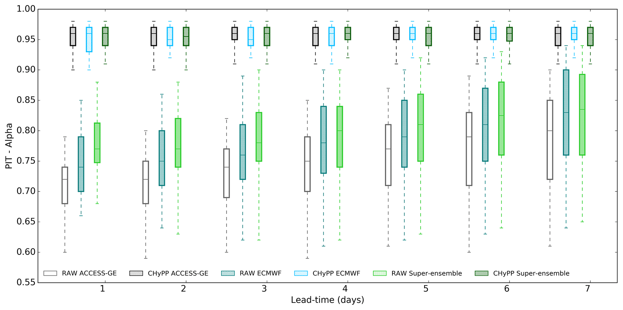
Figure 5Reliability (PIT-alpha) of different rainfall products (raw and calibrated using CHyPP), ACCESS–GE2, ECMWF, and the super-ensemble for the 100 catchments.
The CRPS (error) value is highly related to catchment characteristics. For example, catchments having considerably long dry periods have numerically low average daily CRPS values. Therefore, we present the relative CRPS error (RE) where it is estimated by dividing CRPS by the mean rainfall and converting to a percentage value. Figure 6 shows the distribution of RE for raw and calibrated rainfall forecast products with lead time, where lower error values are better. As expected, RE for all rainfall forecast products (raw and calibrated) increases with lead time while the spread of the error distribution for raw rainfall reduces with lead time. A narrower spread of error distribution over the forecast horizon is observed for all calibrated rainfall products compared to the raw data. Calibration reduces RE at shorter lead times but makes it slightly higher than raw rainfall at long lead times, while increasing the reliability significantly (Fig. 5). Normally calibrated rainfall values are closer to climatology values at long lead times giving more weight to improving the reliability. This is an inherent characteristic of the CHyPP methodology and there is a trade-off between sharpness and reliability. Further research is needed to explore how to keep the balance between the sharpness and reliability of the calibrated forecast rainfall at long lead times.
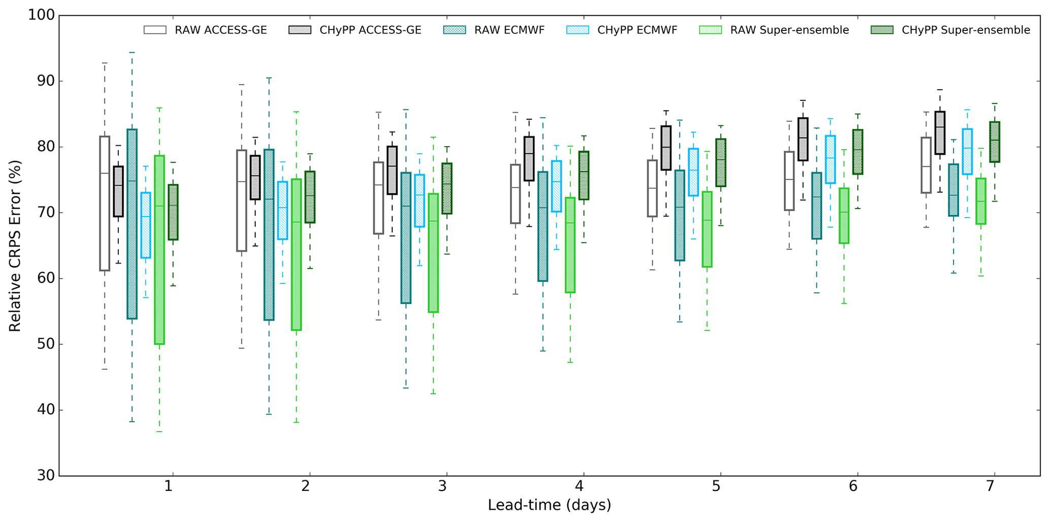
Figure 6Relative CRPS (% of daily observations) of different rainfall products (raw and calibrated using CHyPP), ACCESS–GE2, ECMWF, and the super-ensemble for the 100 catchments.
4.3 Effect of streamflow error modelling
Figure 7 shows bias (%) of streamflow generated before and after error modelling using the ERRIS model with the forecast rainfall super-ensemble (calibrated) for 100 catchments. Bias (%) is calculated for the ensemble median. The bias increases with lead time for both raw and ERRIS-corrected streamflow forecasts. ERRIS-corrected streamflow forecasts (PSFs) demonstrate relatively low bias consistently across all the lead times compared to the raw streamflow forecasts (RSFs) though the magnitude of reduction varies across the continent. PSFs show significantly reduced bias at short lead times for all forecast locations. For lead-day 1, median bias is less than 25 % for all the forecast locations (Fig. 7a), whereas for lead-day 7, the median bias is less than 40 % for about 40 % of forecast locations (Fig. 7b).
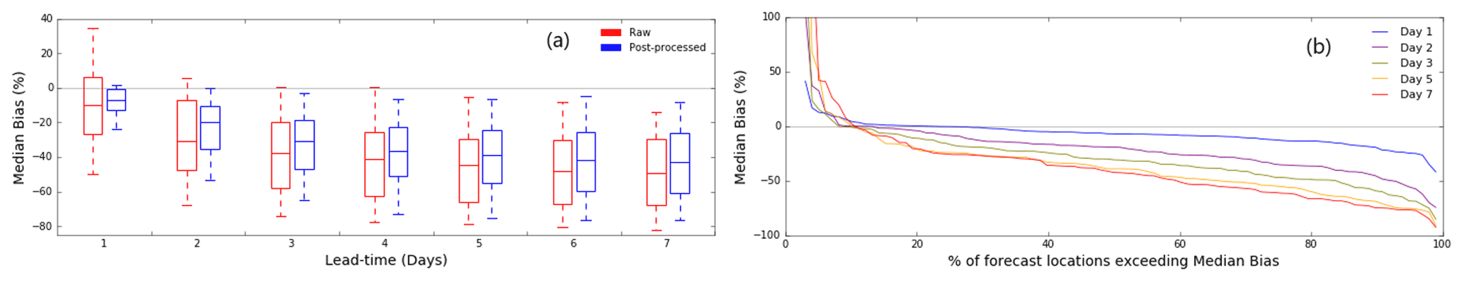
Figure 7(a) Median bias (%) before (raw) and after streamflow error modelling with ERRIS for the 100 forecast locations, and (b) percentage of forecast locations exceeding median bias (%) for ERRIS-corrected streamflow forecasts for different lead times.
The reliability of streamflow forecasts across all catchments is significantly improved consistently over the lead times with ERRIS (Fig. 8a), but the improvement is more prominent for the first 3 d. This improvement could partially be attributed to (i) the effect of streamflow error modelling using ERRIS, and (ii) the improvement in the reliability and reduction of bias in rainfall forecasts. However, the reliability across different catchments, which are located in different hydroclimatic regions (Fig. 4), varies significantly; PIT-alpha is >75 % for more than 80 % of the catchments (Fig. 8b). A wide range of reliability across different forecast locations indicate that ERRIS performance highly relates to specific catchment hydro-climatic characteristics (Table 4).
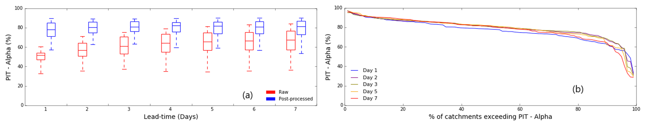
Figure 8(a) Reliability (PIT) before and after streamflow applying ERRIS for the 100 forecast locations, and (b) percentage of forecast locations exceeding PIT (%) for ERRIS-corrected streamflow forecasts for different lead times.
Forecast skill (CRPSS) reduces with lead time for both raw and error-modelled streamflow forecasts (Fig. 9). The degree of improvement of forecast skill provided by error modelling decreases with lead time (Fig. 9a). For lead-day 1, all the forecast locations exceed 50 % CRPSS (Fig. 9b) for error-modelled streamflow. Positive CRPSS means the forecast is considered better than using climatology. For lead-day 7, CRPSS is positive for 60 % of the forecast locations and it is 80 % for lead-day 6. Out of about 40 % forecast locations where CRPSS is negative for lead-days 7, most are located where observation networks are sparse, and the rivers are intermittent or ephemeral due to dry climates. Further details are present in the discussion section.
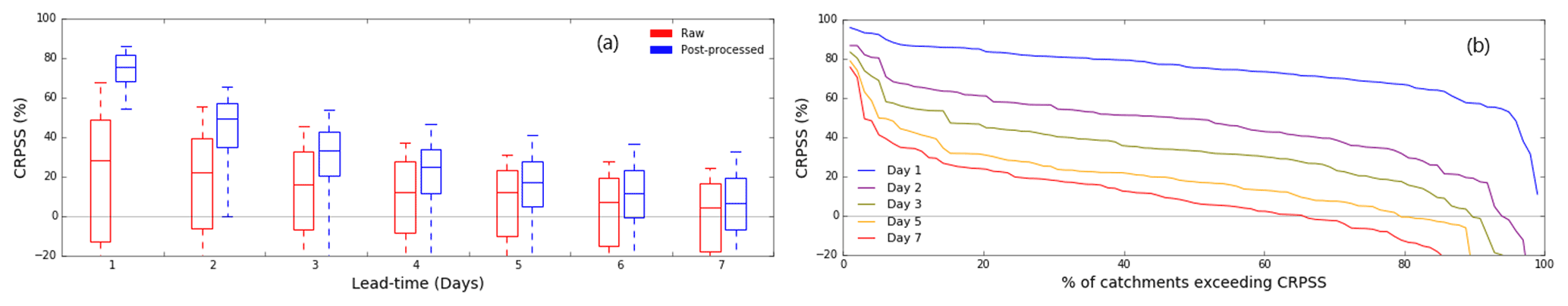
Figure 9(a) CRPSS (%) of streamflow for raw and ERRIS-corrected forecasts, and (b) percentage of forecast locations (total 100) exceeding CRPSS (%) for ERRIS-corrected streamflow forecasts for different lead times.
4.4 Streamflow forecast skill
Forecast skills for hydrologic models are generally low for extreme events that rarely occur, and only a few extreme events are present in a relatively short period (e.g. 3 yr) within the dataset used here. Bootstrapping allows exploration of model forecast skill for a combination of various conditions, such as prolonged wet and/or dry periods, where the sequence of events (e.g. continuously a few wet or dry events) could be absent in the original dataset. Bootstrapped samples of the 3 yr dataset might contain more or fewer wet or dry periods than in the original 3 yr dataset, thus providing a better indication of skill variability across a more realistically varying sample. We test the methodology described in Sect. 2.4 for six catchments. Similar results are found for all the catchments. For the explanation of results, Fig. 10 shows bootstrapped forecast skill for the Acheron River at the Taggerty site for different number of iterations and block sizes. Forecast skill (CRPSS) is sensitive to block size (Fig. 10), and it reduces with lead time for both the weekly-block (w-block) and the monthly-block (m-block) sample sizes. Forecast skill calculated using w-block (Fig. 10a) shows less variation and narrower spread with lead time than when m-block is used (Fig. 10b). For the catchments we tested, the forecast skill is independent of the number of iterations for the w-block size (Fig. 10a). For the m-block size (Fig. 10b), the forecast skill varies with the number of iterations. There is marginal variation in the spread of the skill for iterations 500 and 1000 compared with iterations 100 and 200. This implies that the m-block size captures uncertainty in the forecasts slightly better than the w-block size. Also, the m-block requires fewer computation resources. Therefore, we adopt an m-block size for calculating the forecast skill for the operational service. There is no significant variation of the results for a different number of iterations for both block sizes. This result may be partially attributed to the small sample size of forecast data. To make sure we properly capture uncertainties in skill score calculation, we adopt 500 iterations for the operational service. Note that the block size may be catchment-dependent, e.g. on catchment characteristics such as geomorphology, hydro-climatology, and upstream area. An alternative way of defining a block could be by identifying wet, dry, and normal periods from the original dataset for bootstrapping. However, this process is unique to each catchment, and it is time-consuming to implement for an operational service. Further research is required to investigate block size dependency on catchment characteristics.
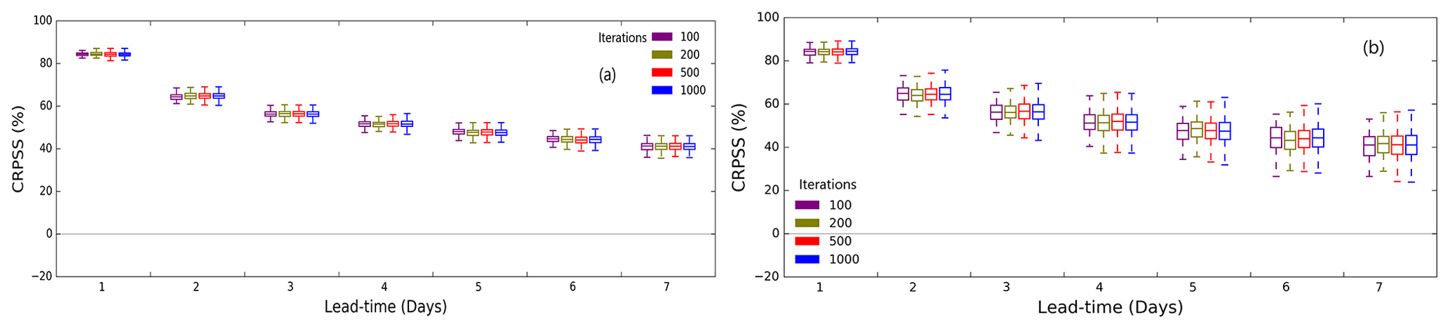
Figure 10Bootstrapped forecast skill for the Acheron River at the Taggerty site for different number of iterations and block sizes – (a) weekly and (b) monthly.
4.5 Acceptance criteria
It is essential for an operational service to maintain a certain standard for the quality of products provided to the users. In consultation with key stakeholders, we developed criteria based on model performance and forecast skill for accepting forecast locations for the operational service. The first criterion is that the Nash–Sutcliffe efficiency (NSE) of simulated streamflow is 0.6 or greater (Chew and McMahon, 1993) for a forecast location in the model validation (see Sect. 2.2.3). This requirement was adopted in consultation with the stakeholders to maintain the service standard. It ensures the hydrological model is robust and produces acceptable results with observed data. If the first criterion is met, then forecast skill (CRPSS), with reference to climatology, should be consecutively positive up to 3 d lead time (Fig. 11). We calculate model performance metrics for each forecast location, and only if the criteria for a forecast location are satisfied, it is added to the public service. Poor quality forecasts possibly lead to miscommunicating the flow conditions with the public. It impacts the reputation of the service and the organisation. If only the first criterion is satisfied, we consider releasing the forecasts only to registered users based on stakeholder requirements and the social and economic importance of forecasts at the location. Some water agencies use their own tools to generate streamflow forecasts. Therefore, consistently maintaining the forecast quality is important for a national operational service. If the first criterion is not met, then the forecast location is unsuitable for the service, and further revision of the model is required. We modelled 283 potential forecast locations in 100 catchments for the current service, and of these, 209 forecast locations in 99 catchments pass the acceptance criteria and are released to the public. On users' request, we relaxed the acceptance criteria for the locations with social and economic significance. A further 17 forecast locations (including one additional catchment) with forecast skill slightly below the acceptance benchmark are released to registered users only.
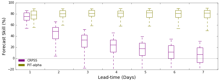
Figure 11Forecast skill (CRPSS %) and reliability (PIT-alpha %) for the 209 forecast locations in the operational public service.
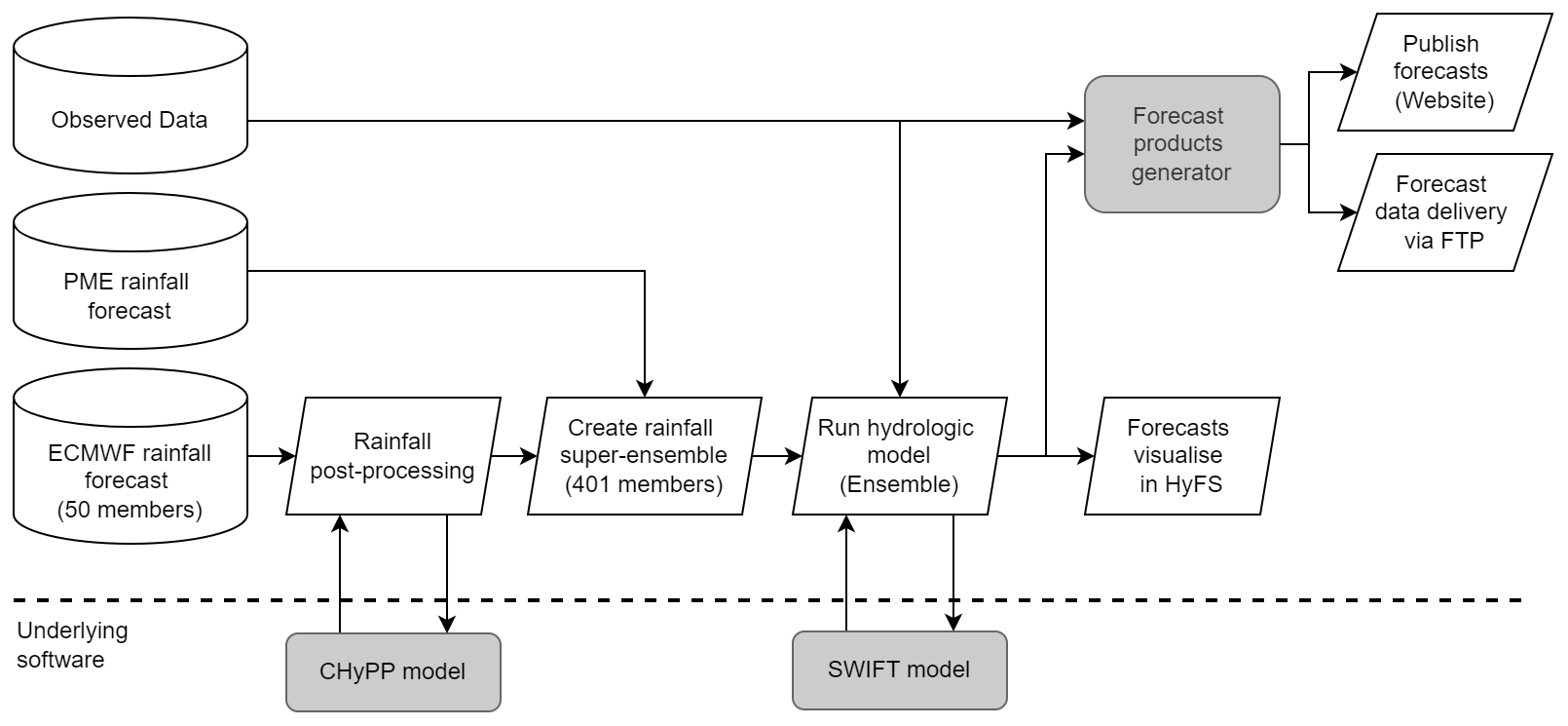
We developed the operational 7-day ensemble streamflow forecasting system based on the evidence derived from the above results. We designed the SDF forecast system to use multi-model rainfall forecasts to improve the quality of streamflow forecasts and minimise the potential risk of system failure due to the absence of NWP rainfall input. The rainfall forecasts used in the SDF service are ECMWF and PME (Fig. 12). We also planned to use the ACCESS–GE product for the service and conducted an extensive evaluation as presented in this paper. However, the operational delivery of the ACCESS–GE had been delayed, and therefore it is to be included in the service in the near future. In the absence of ACCESS–GE data, the CHyPP model is used to calibrate ECMWF forecasts and generate 400 (instead of 200 as described in Sect. 4.1) bias-corrected and statistically reliable hourly rainfall forecast members. We combine calibrated ECMWF and PME rainfall forecasts and input them into the SWIFT model to generate 401 members of hourly streamflow forecasts (Fig. 12) in the operational system. Ensemble streamflow forecasts are fed into a product generator to produce plots, tables, and data files, and publish in a web portal (http://www.bom.gov.au/water/7daystreamflow/, last access: 16 September 2022). In addition to the web plots, users can extract data through the web portal and ingest forecast data to their operational systems via a File Transfer Protocol (FTP) link. The forecasts are generated daily in the BoM's operational platform, Hydrological Forecasting System (HyFS) (Robinson et al., 2016). It is the central national platform that supports flood forecasting and warning as well in Australia. HyFS is a Delft–FEWS-based (flood early warning system) forecasting environment (see https://publicwiki.deltares.nl/display/FEWSDOC/Home, last access: 16 September 2022). HyFS allows ingestion and processing of real-time observations and Numerical Weather Prediction (NWP) model rainfall forecasts, running routine workflows, model internal state management, and forecast visualisation. The process is fully automated (Fig. 12), and forecasts are updated daily between 10:00 and 00:00 AEST.
6.1 Interpretation of forecast skill
Model performance statistics of validation and forecast verification for lead-day 3 for 283 potential forecast locations in the seven jurisdictions of Australia are shown in Table 4. Figure 13 shows the forecast skills (CRPSS %) of the potential forecast locations for lead-days 1 and 3 with the mean annual rainfall in the background. In model validation, South Australia (SA) models have the poorest NSE compared to other jurisdictions. Overall, 40 % of forecast locations in South Australia and 23 % in Western Australia fail the first acceptance criterion (NSE > 0.6) while it is less than 12 % for other jurisdictions. We note that some forecast locations in Western Australia (WA), Tasmania (TAS), and inland areas of New South Wales (NSW), Queensland (QLD), and Victoria (VIC) show poor NSE. These areas have intermittently flowing rivers due to arid or semi-arid climates (see the aridity index in Table 3). Much of continental Australia to the west of the Great Dividing Range (an area of >5 million km2) where the mean annual rainfall is <400 mm (Fig. 13) is sparsely populated and characterised by intermittent and ephemeral streamflows. Therefore, the observation network is also sparse and there is not enough benefit to justify the cost for expanding the observation network. Ephemeral rivers are subject to strongly non-linear relationships that are less well understood in rainfall and runoff, and are inherently more challenging to model than perennial catchments (Gutierrez-Jurado et al., 2021). The forecast skill (CRPSS %) is also poor for SA, inland parts of NSW, and QLD (mean annual rainfall <400 mm), and some parts of VIC and TAS (Fig. 12). For these areas, the forecast skill significantly drops from lead-days 1 to 3. This is partially due to the poor quality of rainfall forecasts (Shresta et al., 2013). Arid regions are generally characterised by high rainfall variability, and often these rainfalls are underestimated by NWP models. It may be difficult for NWP models to replicate the complex meteorological processes that drive the high rainfall variability with limited observations. Therefore, improving forecast skill in ephemeral catchments is likely to remain challenging.
Table 4Hydrologic model performance statistics for 283 forecast locations.
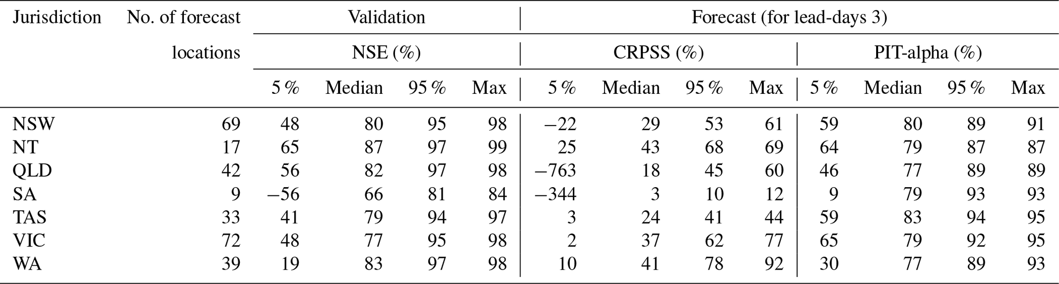
Note: y % is yth percentile, NSW: New South Wales, NT: Northern Territory, QLD: Queensland, SA: South Australia, TAS: Tasmania, VIC: Victoria, and WA: Western Australia. CRPSS and PIT-alpha values are the median of the respective bootstrapped samples.

Figure 13Forecast skill, CRPSS (%) for the 283 forecast locations (a) for lead-days 1 and (b) for lead-days 3. The mean annual rainfall (mm) in Australia is shown in the background.
NWP rainfall calibration using CHyPP reduces bias and increases reliability across all catchments (Figs. 4, 5). In doing so, there is a compromise in relative CRPS – an improvement in shorter lead times but there is no discernible improvement – or in some cases, a slight decline, at longer lead times (Fig. 6). However, relative improvements in forecast skill in ephemeral catchments are less prominent compared with perennial catchments. Similar results were found by Li et al. (2021). These results are discussed with many stakeholders across the country as part of development of the operational service. A clear message from them is that reliable streamflow forecasts are more important than precise forecasts for long lead times to downstream users and will be beneficial to their decision-making.
Streamflow forecast skill calculated using the bootstrapping technique appears to be realistic for most forecast locations. This gives some confidence that we can expect similar performance under operational conditions. However, in this study, bootstrapping is only able to sample within the evaluation period, which is 3 yr from 2014 to 2016. The years 2014 and 2015 were average to dry years for most of the selected catchments, which are located along Australia's coastal regions (Fig. 2). The year 2016 was a wet year for South Australia, Victoria, and Tasmania, where about a half of the selected catchments are located. Overall, there were only a few wet events in the evaluation dataset. Therefore, we recommend that users are cautious when interpreting the forecast skill for wet events. A more extended period of data, with balanced wet and dry events, is recommended for a better evaluation of streamflow forecast skill. In addition, short-term verification statistics on a daily basis will be useful for users for better decision-making.
We demonstrate with various performance measures that calibration adds value to raw NWP rainfall forecasts, and the relative improvement is different for each product. For example, raw ECMWF rainfall is less biased compared to ACCESS–GE2 (Fig. 4). Therefore, the selection of rainfall forecast products for the operational forecasting system may affect the quality of streamflow forecasts (see Sect. 6). In this study, our criteria for selecting NWP rainfall forecast products are availability of the product at the BoM, hindcast period, and ease of use (i.e. format, extent, file size). Where a range of suitable products are available, we recommend conducting a thorough evaluation before selecting NWP products to use.
6.2 Uncertainties in forecasts
Input data (observations and forecasts) and hydrological model structural uncertainties contribute to the streamflow forecast uncertainties. We try to minimise input data uncertainty by calibrating NWP rainfall forecasts using the CHyPP model, and minimise the hydrologic uncertainty by applying the ERRIS error model to simulated discharge. We demonstrate that calibrated NWP rainfall forecasts improve streamflow forecast skill. Similar results are found in Canada and South America (Rogelis and Werner, 2018; Jha et al., 2018). However, uncertainties may also arise from the observed data used to calibrate parameters in the hydrologic models. The most common issues are precision of the instruments that measure the water level (stage) and rainfall, derivation of the stage–discharge relationship (rating tables), the accuracy of gauged rainfall interpolation methods (e.g. inverse distance squared weighted averaging), and data disaggregation methods. Measurement and rating curve uncertainties in streamflow, particularly for low and high flows, bring additional complexities in model calibration/validation and ultimately model performance (Tomkins, 2014).
Although there are many complex methods available for climate data disaggregation (Breinl and Di Baldassarre, 2019; Görner et al., 2021; Mehrotra and Singh, 1998), for simplicity, we use a simple method, linear interpolation for disaggregating daily rainfall and PE data to hourly. PE varies with the diurnal cycle and usually shows some degree of (negative) correlation with rainfall that could have been considered in the disaggregation. However, we note that the impact of rainfall uncertainty has been shown to be more significant than PE in hydrological modelling (Paturel et al., 1995; Guo et al., 2017). The sparseness of the rainfall observation network in much of inland Australia (particularly in the inland desert regions and in northwest Australia) remains a challenge for the development of any streamflow forecasting system.
6.3 Streamflow error modelling method
Modelling hydrological errors using the ERRIS model significantly reduces the bias and improves the forecast skill (Fig. 7). Improvements in forecast skill depend on location, season, and lead time (Hegdahl et al., 2021; Jha et al., 2018). However, calibration of ERRIS is sensitive to the quality of observations (Li et al., 2016). ERRIS uses a log-sinh transformation to normalise streamflow prediction errors, and the transformation amplifies errors related to low simulated flow and modulating errors related to high simulated flow. Therefore, if there are large uncertainties in low streamflow observations, these will result in large residual variances in the transformed space and lead to large forecast uncertainties. As a result, forecasts may be reliable, but have low precision particularly at long lead times.
The ERRIS model applies corrections to hydrological model output, but it does not address the underlying cause of the forecast errors. Relatively simple error models like ERRIS try to characterise prediction errors that arise from many different causes and persist over many different time horizons. For example, error models may try to address: (i) long-term or average forecast errors related to the hydrological model calibration, (ii) forecast errors that persist for intermediate time periods of days to months that may arise from the effects of errors in magnitude of catchment rainfall estimates for a significant event, and (iii) transient errors related to incorrectly assumed diurnal pattern in potential evapotranspiration or small errors in the timing of catchment rainfall. On the other hand, data assimilation methods seek to address underlying causes of some hydrological simulation errors, particularly those that persist over long and intermediate timeframes, by updating model state variables (initial conditions) and forcing, so that model predictions better reflect observations. However, implementation of a data assimilation method for probabilistic streamflow forecasting using a hydrological model is challenging due to (i) the complexity in inter-dependencies of uncertainty contributing sources such as an ensemble of model forcing data, (ii) model state variables and/or model parameters, and (iii) compromise in landscape water balance which may lead to long-term biases in streamflow forecasts (Moradkhani et al., 2005; Li et al., 2016). In a forecasting context, the objective is to ensure that the initial condition set in a hydrological model better reflects reality and therefore forecast errors are likely to be smaller. However, even after updating state variables, hydrological model predictions are unlikely to be perfect, and therefore a role for an error model such as ERRIS in an operational system is still worth exploring. Decreased dependence on error corrections through weaker bias corrections, lower autocorrelation parameters, and lower residual variances when ERRIS is calibrated using updated streamflow forecasts by a data assimilation technique may improve the overall streamflow forecast skill. Further exploration for implementing data assimilation for the service is planned.
6.4 Challenges in operational forecasting and opportunities
Over the last two decades, the number of studies in ensemble streamflow forecasting has increased significantly. However, applications of ensemble forecasting vary significantly in terms of geographical distribution, forecast horizon, methodology, and evaluation. This could partially be due to the evolution of ensemble streamflow forecasting science from research to operations. There are many challenges in the large-scale operational adoption of ensemble streamflow forecasting (Pagano et al., 2014; Wu et al., 2020). Some of these challenges for ensemble streamflow forecasting research, operational application, adoption, and benefit to the community are:
Best use of the available data. In Australia, observed rainfall at a sub-daily timescale is available for most stations. Length of the sub-daily rainfall records vary from one station to another – to a maximum of 50 yr. However, the number of rainfall stations is declining over time, and some of the catchments already have a sparse network. Measurement of PE data is rare across the country. Simulated monthly PE data from the AWAP (Raupach et al., 2009) is disaggregated to hourly for hydrological model application. Streamflow gauging stations where the automated facility is available for reporting in real time are ingested into the BoM system. These observed data are the backbone of the hydrological model construction, calibration, validation, and forecasting. Any improvements in measurement and rating curve uncertainties may result in better performance in streamflow forecasting. Updating measurement stations with automation facilities may result in better quality data which could be useful for more skilful forecasting. This study demonstrates that improvements in NWP rainfall forecasts directly contributes to improvements in streamflow. Any further improvements in NWP rainfall forecasts will result in more accurate and reliable streamflow predictions. Possible improvements in different flow regimes, particularly low and high flows, will be explored in the future. Endeavours should also be undertaken to explore emerging science, including merging radar rainfall with NWP forecasts (Velasco-Forero et al., 2021).
Extending the forecast horizon. In addition to the 7 d ahead forecasts, the Bureau also provides operational seasonal predictions (http://www.bom.gov.au/water/ssf/index.shtml, last access: 16 September 2022) from 1 to 3 months ahead (Woldemeskel et al., 2018). Potentially the gap between these two forecast ranges could be minimised by extending the 7 d streamflow forecasts to multi-week forecasts. Rainfall forecast data to at least 30 d ahead are now available, and the multi-model ensemble approach could be used to increase the predictability and reliability of these rainfall forecasts (Specq et al., 2020). The potential use of the rainfall forecast data for extending the streamflow forecasts to 30 d ahead could be explored in the future. A novel Multi-Temporal Hydrological Residual Error (MuTHRE) model (McInerney et al., 2020) has been recently developed to enable reliable streamflow forecasting beyond one week. The model has been tested for 11 catchments to generate sub-seasonal forecasts (lead time 1–30 d) using the GR4J hydrologic model and calibrated rainfall forecasts from the ACCESS–seasonal NWP model (McInerney et al., 2020). They found that forecast performance was improved compared to the current seasonal streamflow forecasts in terms of sharpness, volumetric bias, and skill. This approach could be further explored for wider-scale applications across Australia for seamless streamflow forecasting.
Forecasting in managed river systems. At present, the BoM's operational streamflow forecasting services do not receive real-time and future water releases from dams and reservoirs. Therefore, the 7 d streamflow forecasting service is developed for catchments with minimal or no anthropogenic influences (e.g. releases from storage, extractions). Catchments in this study (Fig. 2) are all upstream of dams, reservoirs, or weirs, and have no significant water extraction or irrigation return flows. Further investigation to account for these anthropogenic processes will lead to greater expansion and application of the forecast service. Research should be conducted to understand how these anthropogenic influences impact the forecasts, and incorporate practical and innovative solutions into the hydrological forecasting models.
Effective communication. The 7 d ensemble streamflow forecasting service produces large volumes of information. Therefore, key messages must be conveyed clearly and efficiently for correct interpretation, allowing for well-informed decision-making and common understanding among end-user communities. The user communities in Australia range from experts in water management in decision-making entities to those with no experience in using ensemble forecast products. To effectively communicate forecasts with end users in mind, the BoM consults widely and frequently with stakeholders, considers their needs, and provides clear and effective forecast visualisations, including the website and forecast products. The BoM continually improves the forecast products through stakeholder consultation and feedback.
Maintaining operational service. Maintaining the operational 7 d streamflow forecasting service is a big task – and requires a well-trained, dedicated team of staff with expert knowledge of the catchments, and experience with hydrologic model application and forecast system configuration. Particularly, if poor quality observed rainfall and discharge data are used in a model, we find discontinuity in the output when transitioning from simulation to forecast due to the instability of the ERRIS model. If this occurs, the model is taken temporarily out of the service by the monitoring team, and the user community is notified through the website. Losing in-house modelling or systems expertise due to limited funding or incentives may result in suboptimal forecast quality and end-user benefits.
Each of these challenges shares a real-world perspective and its relative importance varies across different geographical regions of Australia. It opens ongoing research and development opportunities, resulting in a greater update of ensemble streamflow forecasting for operational decision-making.
We present the development of a 7 d ensemble streamflow forecasting service for Australia (http://www.bom.gov.au/water/7daystreamflow/, last access: 16 September 2022). The service has been operational since December 2019 and provides daily updates of streamflow forecasts up to 7 lead days for 209 forecast locations in 99 catchments for the public and an additional 17 forecast locations including one catchment to the registered users. The forecast system is capable of ingesting and calibrating multi-model ensemble NWP rainfall forecasts using the CHyPP model, which combines a Bayesian joint probability model and the Schaake Shuffle method. Calibrated ensemble rainfall forecasts are fed into a hydrological modelling package, SWIFT, which then generates error-corrected ensemble streamflow forecasts.
We show that calibrating NWP rainfall forecasts using the CHyPP model significantly reduces bias and improves reliability. Error modelling of streamflow forecasts using ERRIS further improves their accuracy and reliability. A sensitivity analysis for optimising the number of streamflow ensemble members for the operational service shows that more than 200 members are needed to represent the forecast uncertainty. We show that the bootstrapping block size is sensitive to the forecast skill calculation and a month is better than a week as the monthly block size allows to capture maximum possible uncertainty. Acceptance criteria are defined based on model validation and verification results for selecting locations with an adequate forecast quality for the operational service. The acceptance criteria are defined as an NSE greater than 0.6 in model validation, and a median of bootstrapped model verification skill (CRPSS) that is positive (greater than zero) for consecutive 3 d lead time. Incorporation of ACCESS–GE3 rainfall forecasts into the operational service is planned, and continued stakeholder feedback will be used to guide further enhancements of the service.
Code and software used in the operational service are not available for the public. However, the output results can be provided on request via the the “Feedback” page of the 7-day ensemble streamflow forecast website: http://www.bom.gov.au/water/7daystreamflow/ (last access: 16 September 2022).
HAPH designed all experiments with support from all authors. AK, MMH, NG, FMW, XSZ, and HAPH contributed to data extraction, quality checking, catchment delineation, model setup, and cross-validation. MMH conducted all NWP rainfall evaluation experiments and prepared results. AK conducted all streamflow evaluation experiments and prepared results. NG conducted geo-spatial analysis and prepared maps. PDS led the upgrade of information systems for the ensemble forecasting capability, including workflows and data-processing tools, archiving sub-system, a forecast products generator, web interface improvements, and integration into HyFS/FEWS. HAPH and MAB analysed the results and prepared the paper with contributions from all authors. PMF and MAB provided project administration, resource allocation, and scientific editing support. DER and JCB contributed to the development of the methodology and reviewed the paper.
The contact author has declared that none of the authors has any competing interests.
Publisher's note: Copernicus Publications remains neutral with regard to jurisdictional claims in published maps and institutional affiliations.
We acknowledge funding from the Water Information Research and Development Alliance (WIRADA) for the SWIFT model development and the underlying research. We thank colleagues in the Bureau of Meteorology from Water Forecasting Services, HyFS, systems support, Data and Digital, and Science and Innovation for their support in developing this operational service. We acknowledge the national and state water agencies across Australia for providing gauged data, critical catchment information for modelling, and their input for forecast location selection and products design. The operational website was developed in consultation with the CSIRO and approximately 70 other stakeholders across Australia. We would like to express our sincere thanks to our technical reviewers Beth Ebert, Christoph Rudiger, and Elisabetta Carrara for their time, careful review, and valuable comments and suggestions on the submitted version of this paper. The technical advice and management support received from Narendra K. Tuteja and Daehyok Shin are sincerely acknowledged. The large computations in this study were conducted using the facilities provided by the National Computational Infrastructure (NCI) supported by the Australian Government.
This paper was edited by Yi He and reviewed by two anonymous referees.
Alfieri, L., Burek, P., Dutra, E., Krzeminski, B., Muraro, D., Thielen, J., and Pappenberger, F.: GloFAS – global ensemble streamflow forecasting and flood early warning, Hydrol. Earth Syst. Sci., 17, 1161–1175, https://doi.org/10.5194/hess-17-1161-2013, 2013.
Andréassian, V.: Waters and forests: From historical controversy to scientific debate, J. Hydrol., 291, 1–27, https://doi.org/10.1016/j.jhydrol.2003.12.015, 2004.
Atkinson, R., Power, R., Lemon, D., O'Hagan, R., Dovey, D., and Kinny, D.: The Australian Hydrological Geospatial Fabric – Development Methodology and Conceptual Architecture, Canberra, Australia, 60 pp., https://doi.org/10.4225/08/585ac46ee9981, 2008.
Bennett, J. C., Robertson, D. E., Shrestha, D. L., Wang, Q. J., Enever, D., Hapuarachchi, P., and Tuteja, N. K.: A System for Continuous Hydrological Ensemble Forecasting (SCHEF) to lead times of 9 days, J. Hydrol., 219, 2832–2846, https://doi.org/10.1016/j.jhydrol.2014.08.010, 2014.
Bennett, J. C., Robertson, D. E., Ward, P. G. D. D., Hapuarachchi, H. A. A. P., and Wang, Q. J. J.: Calibrating hourly rainfall-runoff models with daily forcings for streamflow forecasting applications in meso-scale catchments, Environ. Model. Softw., 76, 20–36, https://doi.org/10.1016/j.envsoft.2015.11.006, 2016.
Bennett, J. C., Wang, Q. J., Robertson, D. E., Schepen, A., Li, M., and Michael, K.: Assessment of an ensemble seasonal streamflow forecasting system for Australia, Hydrol. Earth Syst. Sci., 21, 6007–6030, https://doi.org/10.5194/hess-21-6007-2017, 2017.
Bennett, J. C., Robertson, D. E., Wang, Q. J., Li, M., and Perraud, J. M.: Propagating reliable estimates of hydrological forecast uncertainty to many lead times, J. Hydrol., 603, 126798, https://doi.org/10.1016/j.jhydrol.2021.126798, 2021.
Bierkens, M. F. P., Bell, V. A., Burek, P., Chaney, N., Condon, L. E., David, C. H., de Roo, A., Döll, P., Drost, N., Famiglietti, J. S., Flörke, M., Gochis, D. J., Houser, P., Hut, R., Keune, J., Kollet, S., Maxwell, R. M., Reager, J. T., Samaniego, L., Sudicky, E., Sutanudjaja, E. H., van de Giesen, N., Winsemius, H., and Wood, E. F.: Hyper-resolution global hydrological modelling: what is next?, Hydrol. Process., 29, 310–320, https://doi.org/10.1002/hyp.10391, 2015.
Breinl, K. and Di Baldassarre, G.: Space-time disaggregation of precipitation and temperature across different climates and spatial scales, J. Hydrol. Reg. Stud., 21, 126–146, https://doi.org/10.1016/j.ejrh.2018.12.002, 2019.
Buizer, J., Jacobs, K., and Cash, D.: Making short-term climate forecasts useful: Linking science and action, P. Natl. Acad. Sci. USA, 113, 4597–4602, https://doi.org/10.1073/pnas.0900518107, 2016.
Charles, S. P., Wang, Q. J., Ahmad, M.-D., Hashmi, D., Schepen, A., Podger, G., and Robertson, D. E.: Seasonal streamflow forecasting in the upper Indus Basin of Pakistan: an assessment of methods, Hydrol. Earth Syst. Sci., 22, 3533–3549, https://doi.org/10.5194/hess-22-3533-2018, 2018.
Clark, M., Gangopadhyay, S., Hay, L., Rajagopalan, B., and Wilby, R.: The Schaake shuffle: A method for reconstructing space-time variability in forecasted precipitation and temperature fields, J. Hydrometeorol., 5, 243–262, https://doi.org/10.1175/1525-7541(2004)005<0243:TSSAMF>2.0.CO;2, 2004.
Coron, L., Andréassian, V., Perrin, C., Lerat, J., Vaze, J., Bourqui, M., and Hendrickx, F.: Crash testing hydrological models in contrasted climate conditions: An experiment on 216 Australian catchments, Water Resour. Res., 48, W05552, https://doi.org/10.1029/2011WR011721, 2012.
Delaney, C. J., Hartman, R. K., Mendoza, J., Dettinger, M., Delle Monache, L., Jasperse, J., Ralph, F. M., Talbot, C., Brown, J., Reynolds, D., and Evett, S.: Forecast Informed Reservoir Operations Using Ensemble Streamflow Predictions for a Multipurpose Reservoir in Northern California, Water Resour. Res., 56, e2019WR02660, https://doi.org/10.1029/2019WR026604, 2020.
Demargne, J., Wu, L., Regonda, S. K., Brown, J. D., Lee, H., He, M., Seo, D. J., Hartman, R., Herr, H. D., Fresch, M., Schaake, J., and Zhu, Y.: The science of NOAA's operational hydrologic ensemble forecast service, B. Am. Meteorol. Soc., 95, 79–98, https://doi.org/10.1175/BAMS-D-12-00081.1, 2014.
Duan, Q., Sorooshian, S., and Gupta, V. K.: Optimal use of the SCE-UA global optimization method for calibrating watershed models, J. Hydrol., 158, 3–4, https://doi.org/10.1016/0022-1694(94)90057-4, 1994.
Ebert, E. E.: Ability of a poor man's ensemble to predict the probability and distribution of precipitation, Mon. Weather Rev., 129, 2461–2480, https://doi.org/10.1175/1520-0493(2001)129<2461:AOAPMS> 2.0.CO;2, 2001.
Efron, B. and Tibshirani, R. J.: An Introduction to the Bootstrap (1st Ed.), Chapman and Hall/CRC, New York, USA, 1994.
Emerton, R. E., Stephens, E. M., Pappenberger, F., Pagano, T. C., Weerts, A. H., Wood, A. W., Salamon, P., Brown, J. D., Hjerdt, N., Donnelly, C., Baugh, C. A., and Cloke, H. L.: Continental and global scale flood forecasting systems, WIREs Water, 3, 391–418, https://doi.org/10.1002/wat2.1137, 2016.
Görner, C., Franke, J., Kronenberg, R., Hellmuth, O., and Bernhofer, C.: Multivariate non-parametric Euclidean distance model for hourly disaggregation of daily climate data, Theor. Appl. Climatol., 143, 241–265, https://doi.org/10.1007/s00704-020-03426-7, 2021.
Guo, B., Xu, T., Zhang, J., Croke, B., Jakeman, A., Seo, L., Lei, X., and Liao, W.: A comparative analysis of precipitation estimation methods for streamflow prediction, in: Proceedings - 22nd International Congress on Modelling and Simulation, Modelling and Simulation Society of Australia and New Zealand, Hobart, Tasmania, Australia, 3-8 December 2017, 43–49, https://doi.org/10.36334/modsim.2017.a1.guo, 2017.
Gutierrez-Jurado, K. Y., Partington, D., and Shanafield, M.: Taking theory to the field: streamflow generation mechanisms in an intermittent Mediterranean catchment, Hydrol. Earth Syst. Sci., 25, 4299–4317, https://doi.org/10.5194/hess-25-4299-2021, 2021.
Hapuarachchi, H. A. P., Kabir, A., Zhang, S., Tuteja, N., Enever, D., Kent, D., Bari, M., Shin, D., Laugesen, R., and Amirthanathan, G.: Development of an operational system for the 7-day streamflow forecast service in Australia, in: Ozwater, 2016 .
Hegdahl, T. J., Engeland, K., Steinsland, I., and Singleton, A.: The benefits of pre- and postprocessing streamflow forecasts for an operational flood-forecasting system of 119 Norwegian catchments, Hydrol. Earth Syst. Sci. Discuss. [preprint], https://doi.org/10.5194/hess-2021-13, 2021.
Hersbach, H.: Decomposition of the continuous ranked probability score for ensemble prediction systems, Weather Forecast., 15, 559–570, https://doi.org/10.1175/1520-0434(2000)015< 0559:DOTCRP>2.0.CO;2, 2000.
Jha, S. K., Shrestha, D. L., Stadnyk, T. A., and Coulibaly, P.: Evaluation of ensemble precipitation forecasts generated through post-processing in a Canadian catchment, Hydrol. Earth Syst. Sci., 22, 1957–1969, https://doi.org/10.5194/hess-22-1957-2018, 2018.
Kunnath-Poovakka, A. and Eldho, T. I.: A comparative study of conceptual rainfall-runoff models GR4J, AWBM and Sacramento at catchments in the upper Godavari River basin, India, J. Earth Syst. Sci., 128, 33, https://doi.org/10.1007/s12040-018-1055-8, 2019.
Laio, F. and Tamea, S.: Verification tools for probabilistic forecasts of continuous hydrological variables, Hydrol. Earth Syst. Sci., 11, 1267–1277, https://doi.org/10.5194/hess-11-1267-2007, 2007.
Li, M., Wang, Q. J., Bennett, J. C., and Robertson, D. E.: Error reduction and representation in stages (ERRIS) in hydrological modelling for ensemble streamflow forecasting, Hydrol. Earth Syst. Sci., 20, 3561–3579, https://doi.org/10.5194/hess-20-3561-2016, 2016.
Li, M., Robertson, D. E., Wang, Q. J., Bennett, J. C., and Perraud, J. M.: Reliable hourly streamflow forecasting with emphasis on ephemeral rivers, J. Hydrol., 598, 125739, https://doi.org/10.1016/j.jhydrol.2020.125739, 2021.
McInerney, D., Thyer, M., Kavetski, D., Laugesen, R., Tuteja, N., and Kuczera, G.: Multi-temporal Hydrological Residual Error Modeling for Seamless Subseasonal Streamflow Forecasting, Water Resour. Res., 56, e2019WR026979, https://doi.org/10.1029/2019WR026979, 2020.
Mehrotra, R. and Singh, R. D.: Spatial disaggregation of rainfall data, Hydrol. Sci. J., 43, 91–102, https://doi.org/10.1080/02626669809492104, 1998.
Moradkhani, H., Hsu, K. L., Gupta, H., and Sorooshian, S.: Uncertainty assessment of hydrologic model states and parameters: Sequential data assimilation using the particle filter, Water Resour. Res., 41, W05012, https://doi.org/10.1029/2004WR003604, 2005.
Niu, W. J., Feng, Z. K., Yang, W. F., and Zhang, J.: Short-term streamflow time series prediction model by machine learning tool based on data preprocessing technique and swarm intelligence algorithm, Hydrol. Sci. J., 65, 2590–2603, https://doi.org/10.1080/02626667.2020.1828889, 2020.
O'Kane, T. J., Naughton, M. J., and Xiao, Y.: The Australian community climate and earth system simulator global and regional ensemble prediction scheme, ANZIAM J., 50, 385–398, https://doi.org/10.21914/anziamj.v50i0.1421, 2008.
Pagano, T. C., Wood, A. W., Ramos, M.-H., Cloke, H. L., Pappenberger, F., Clark, M. P., Cranston, M., Kavetski, D., Mathevet, T., Sorooshian, S., and Verkade, J. S.: Challenges of Operational River Forecasting, J. Hydrometeorol., 15, 1692–1707, https://doi.org/10.1175/jhm-d-13-0188.1, 2014.
Pagano, T. C., Shrestha, D. L., Wang, Q. J., Robertson, D., and Hapuarachchi, P.: Ensemble dressing for hydrological applications, Hydrol. Process., 27, 106–116, https://doi.org/10.1002/hyp.9313, 2013.
Pappenberger, F., Pagano, T. C., Brown, J. D., Alfieri, L., Lavers, D. A., Berthet, L., Bressand, F., Cloke, H. L., Cranston, M., Danhelka, J., Demargne, J., Demuth, N., de Saint-Aubin, C., Feikema, P. M., Fresch, M. A., Garçon, R., Gelfan, A., He, Y., Hu, Y.-Z., Janet, B., Jurdy, N., Javelle, P., Kuchment, L., Laborda, Y., Langsholt, E., Le Lay, M., Li, Z. J., Mannessiez, F., Marchandise, A., Marty, R., Meißner, D., Manful, D., Organde, D., Pourret, V., Rademacher, S., Ramos, M.-H., Reinbold, D., Tibaldi, S., Silvano, P., Salamon, P., Shin, D., Sorbet, C., Sprokkereef, E., Thiemig, V., Tuteja, N. K., van Andel, S. J., Verkade, J. S., Vehviläinen, B., Vogelbacher, A., Wetterhall, F., Zappa, M., Van der Zwan, R. E., and Thielen-del Pozo, J.: Hydrological Ensemble Prediction Systems Around the Globe, in: Handbook of Hydrometeorological Ensemble Forecasting, Springer, Berlin, Heidelberg, https://doi.org/10.1007/978-3-642-40457-3_47-1, 2016.
Paturel, J. E., Servat, E., and Vassiliadis, A.: Sensitivity of conceptual rainfall-runoff algorithms to errors in input data – case of the GR2M model, J. Hydrol., 168, 111–125, https://doi.org/10.1016/0022-1694(94)02654-T, 1995.
Perraud, J. M., Bridgart, R., Bennett, J. C., and Robertson, D.: Swift2: High performance software for short-medium term ensemble streamflow forecasting research and operations, in: Proceedings – 21st International Congress on Modelling and Simulation, Modelling and Simulation Society of Australia and New Zealand, Gold Coast, Australia, 29 Nov–4 Dec 2015, 2458–2464, https://doi.org/10.36334/modsim.2015.l15.perraud, 2015.
Perrin, C., Michel, C., and Andréassian, V.: Improvement of a parsimonious model for streamflow simulation, J. Hydrol., 279, 275–289, https://doi.org/10.1016/S0022-1694(03)00225-7, 2003.
Poff, N. L. R., Olden, J. D., Pepin, D. M., and Bledsoe, B. P.: Placing global stream flow variability in geographic and geomorphic contexts, River Res. Appl., 22, 149–166, https://doi.org/10.1002/rra.902, 2006.
Raupach, M. R., Briggs, P. R., Haverd, V., King, E. A., Paget, M., and Trudinger, C. M.: Australian Water Availability Project (AWAP): CSIRO Marine and Atmospheric Research Component: Final Report for Phase 3: CAWCR Technical Report No. 13, Centre for Australian Weather and Climate Research, http://hdl.handle.net/102.100.100/115368?index=1 (last access: 26 September 2022), 2009.
Richardson, D. S.: Skill and relative economic value of the ECMWF ensemble prediction system, Q. J. Roy. Meteor. Soc., 126, 649–667, https://doi.org/10.1002/qj.49712656313, 2000.
Robertson, D. E. and Wang, Q. J.: A Bayesian approach to predictor selection for seasonal streamflow forecasting, J. Hydrometeorol., 13, 155–171, https://doi.org/10.1175/JHM-D-10-05009.1, 2012.
Robertson, D. E., Shrestha, D. L., and Wang, Q. J.: Post-processing rainfall forecasts from numerical weather prediction models for short-term streamflow forecasting, Hydrol. Earth Syst. Sci., 17, 3587–3603, https://doi.org/10.5194/hess-17-3587-2013, 2013.
Robinson, J., Leahy, C., Boronkay, A., and Pierotti, S.: Introducing the Bureau’S New Hydrological Forecasting System, in: Floodplain Management Association National Conference, 1–16, 2016.
Rogelis, M. C. and Werner, M.: Streamflow forecasts from WRF precipitation for flood early warning in mountain tropical areas, Hydrol. Earth Syst. Sci., 22, 853–870, https://doi.org/10.5194/hess-22-853-2018, 2018.
Roy, T., Serrat-Capdevila, A., Valdes, J., Durcik, M., and Gupta, H.: Design and implementation of an operational multimodel multiproduct real-time probabilistic streamflow forecasting platform, J. Hydroinfo., 19, 911–919, https://doi.org/10.2166/hydro.2017.111, 2017.
Shmueli, G.: To explain or to predict?, Stat. Sci., 25, 289–310, https://doi.org/10.1214/10-STS330, 2010.
Siddique, R. and Mejia, A.: Ensemble streamflow forecasting across the U.S. Mid-Atlantic Region with a distributed hydrological model forced by GEFS reforecasts, J. Hydrometeorol., 18, 1905–1928, https://doi.org/10.1175/JHM-D-16-0243.1, 2017.
Smith, P. J., Pappenberger, F., Wetterhall, F., Thielen del Pozo, J., Krzeminski, B., Salamon, P., Muraro, D., Kalas, M., and Baugh, C.: Chapter 11 - On the Operational Implementation of the European Flood Awareness System (EFAS), edited by: Adams, T. E. and Pagano, T. C. B. T.-F. F., Academic Press, Boston, 313–348, https://doi.org/10.1016/B978-0-12-801884-2.00011-6, 2016.
Specq, D., Batté, L., Déqué, M., and Ardilouze, C.: Multimodel Forecasting of Precipitation at Subseasonal Timescales Over the Southwest Tropical Pacific, Earth Sp. Sci., 7, e2019EA001003, https://doi.org/10.1029/2019EA001003, 2020.
Stern, H., De Hoedt, G., and Ernst, J.: Objective classification of Australian climates, Aust. Meteorol. Mag., 49, 87–96, 2000.
Talukder, B. and Hipel, K. W.: Diagnosis of sustainability of trans-boundary water governance in the Great Lakes basin, World Dev., 129, 104855, https://doi.org/10.1016/j.worlddev.2019.104855, 2020.
Tomkins, K. M.: Uncertainty in streamflow rating curves: Methods, controls and consequences, Hydrol. Process., 24, 464–481, https://doi.org/10.1002/hyp.9567, 2014.
Van Dijk, A. I. J. M., Beck, H. E., Crosbie, R. S., De Jeu, R. A. M., Liu, Y. Y., Podger, G. M., Timbal, B., and Viney, N. R.: The Millennium Drought in southeast Australia (2001–2009): Natural and human causes and implications for water resources, ecosystems, economy, and society, Water Resour. Res., 49, 1040–1057, https://doi.org/10.1002/wrcr.20123, 2013.
van Esse, W. R., Perrin, C., Booij, M. J., Augustijn, D. C. M., Fenicia, F., Kavetski, D., and Lobligeois, F.: The influence of conceptual model structure on model performance: a comparative study for 237 French catchments, Hydrol. Earth Syst. Sci., 17, 4227–4239, https://doi.org/10.5194/hess-17-4227-2013, 2013.
Velasco-Forero, C., Pudashine, J., Curtis, M., and Seed, A.: Probabilistic precipitation nowcast for flash flooding purposes across Australia: verification of a new version of Short-Term Ensemble Prediction System (STEPS), in: EGU General Assembly Conference Abstracts, EGU21-13673, 2021.
Verkade, J. S., Brown, J. D., Davids, F., Reggiani, P., and Weerts, A. H.: Estimating predictive hydrological uncertainty by dressing deterministic and ensemble forecasts; a comparison, with application to Meuse and Rhine, J. Hydrol., 555, 257–277, https://doi.org/10.1016/j.jhydrol.2017.10.024, 2017.
Woldemeskel, F., McInerney, D., Lerat, J., Thyer, M., Kavetski, D., Shin, D., Tuteja, N., and Kuczera, G.: Evaluating post-processing approaches for monthly and seasonal streamflow forecasts, Hydrol. Earth Syst. Sci., 22, 6257–6278, https://doi.org/10.5194/hess-22-6257-2018, 2018.
Wu, W., Emerton, R., Duan, Q., Wood, A. W., Wetterhall, F., and Robertson, D. E.: Ensemble flood forecasting: Current status and future opportunities, 62, e1432, https://doi.org/10.1002/wat2.1432, 2020.
Zhao, T., Schepen, A., and Wang, Q. J.: Ensemble forecasting of sub-seasonal to seasonal streamflow by a Bayesian joint probability modelling approach, J. Hydrol., 541, 839–849, https://doi.org/10.1016/j.jhydrol.2016.07.040, 2016.
- Abstract
- Introduction
- Modelling methodology
- Catchment selection and data
- Results
- Description of the operational forecast system
- Discussion and future work
- Summary and conclusions
- Code and data availability
- Author contributions
- Competing interests
- Disclaimer
- Acknowledgements
- Review statement
- References