Technical note: Do different projections matter for the Budyko framework?

The widely used Budyko framework defines the water and energy limits of catchments. Generally, catchments plot close to these physical limits, and Budyko (1974) developed a curve that predicted the positions of catchments in this framework. Often, the independent variable is defined as an aridity index, which is used to predict the ratio of actual evaporation over precipitation ($E_{\mathrm{a}}/P$). However, the framework can be formulated with the potential evaporation as the common denominator for the dependent and independent variables, i.e., $P/E_{\mathrm{p}}$ and $E_{\mathrm{a}}/E_{\mathrm{p}}$. It is possible to mathematically convert between these formulations, but if the parameterized Budyko curves are fit to data, the different formulations could lead to differences in the resulting parameter values. Here, we tested this for 357 catchments across the contiguous United States.

In this way, we found that differences in n values due to the projection used could be ± 0.2. If robust fitting algorithms were used, the differences in n values reduced but were nonetheless still present. The distances to the curve, often used as a metric in Budyko-type analyses, systematically depended on the projection, with larger differences for the non-contracted sides of the framework (i.e., $E_{\mathrm{p}}/P>\mathrm{1}$ or $P/E_{\mathrm{p}}>\mathrm{1}$). When using the two projections for predicting E_a, we found that uncertainties due to the projections used could exceed 1.5 %. An important reason for the differences in n values, curves and resulting estimates of E_a could be found in data points that clearly appear as outliers in one projection but less so in the other projection.

We argue here that the non-contracted side of the framework in the two projections should always be assessed, especially for data points that appear as outliers. At least, one should consider the additional uncertainty of the projection and assess the robustness of the results in both projections.

1 Introduction

Budyko (1974) defined the water and energy limits of catchments in a simple framework and found that most catchments plot close to these limits. He defined a curve through these observations, which is known as the Budyko curve. The framework and curve are widely applied, and the original work of Budyko (1974) has been cited over 3100 times (Google Scholar). Besides that, Budyko's approach finds itself currently in a renaissance, as can be noted by the large number of studies related to the Budyko framework over the recent years. The strength of the approach is widely acknowledged, and especially its simplicity is appealing.

Even though often referred to as the Budyko framework, the base of the framework was formed by the work of Ol'Dekop (1911) and Schreiber (1904). Initially, Schreiber (1904) formulated an exponential function to calculate the runoff ratio of a catchment but only as a function of precipitation and a constant, catchment-specific parameter. Ol'Dekop (1911) added evaporation to this equation but also formulated his own hyperbolic tangent function. Budyko (1974) took later the arithmetic mean of the exponential function and the hyperbolic tangent function, which both had no parameters, to adjust the curve. This was changed by Turc (1954) in France and independently in the Soviet Union by Mezentsev (1955), who both introduced an adjustable exponent. This parameterized form was adopted later by others, in more general formulations, e.g., Fu (1981), Zhang et al. (2001), and Roderick and Farquhar (2011). These formulations often use one single parameter to adjust the curve to the observations. See also Andréassian and Sari (2019) for more details about the historical perspective.

More recently, the Budyko framework has gained popularity with several studies that use the framework for water balance assessment (e.g.,  Andréassian and Perrin, 2012; Coron et al., 2015), model constraining (e.g.,  Nijzink et al., 2018; Hulsman et al., 2018; Mianabadi et al., 2019; Greve et al., 2020) or the assessment of climate change effects (e.g.,  van der Velde et al., 2014; Bouaziz et al., 2022). In addition, several studies exist that adjust the framework for different timescales (Zhao et al., 2020; Wang et al., 2022) or different application fields (Sankarasubramanian et al., 2020).

A large number of studies consider the parameter in the Budyko framework to be catchment-specific and a function of local catchment characteristics. It has been argued that this parameter explains local climatic and environmental conditions combined (e.g.,  Roderick and Farquhar, 2011), but it is often also related to vegetation (e.g.,  Yang et al., 2009; Li et al., 2013; Ning et al., 2017), land cover (Oudin et al., 2008) or human activities (Liang et al., 2015; Yang et al., 2020). Moreover, Zhang et al. (2001) defined n specifically as the plant-available water coefficient. In addition to vegetation, Donohue et al. (2012) related the parameter to multiple variables including storm depths and soil water storage capacities. Furthermore, seasonality is often considered as well as a factor that influences this parameter (Shao et al., 2012; Ning et al., 2017).

Budyko formulated his curve with an aridity index as the independent variable, and most other publications followed that definition. From the older and traditionally cited publications, only Turc (1954) and Pike (1964) formulated the framework with potential evaporation as the common denominator and $P/E_{\mathrm{p}}$ as the independent variable (Andréassian et al., 2016). Nowadays, most publications still use a form of the Budyko framework with the dryness or aridity index $E_{\mathrm{p}}/P$ to predict the dependent variable $E_{\mathrm{a}}/P$, similar as Budyko, but a substantial number of papers use $P/E_{\mathrm{p}}$ as an independent variable to predict the ratio of $E_{\mathrm{a}}/E_{\mathrm{p}}$. Here we refer to these different ways of expressing the dependent and independent variables in the Budyko framework as dryness index and wetness index projections, respectively. These two projections are only discussed in combination in very few studies (e.g.,  Moussa and Lhomme, 2016; Porporato, 2022).

The choice of the projection may depend on the purpose of a given study. Often, the projection with an aridity index is used as it allows for a straightforward estimation of the runoff ratio ($Q/P=\mathrm{1}-E_{\mathrm{a}}/P$), which can, for example, be used directly for constraining hydrological models (e.g.,  Nijzink et al., 2018; Hulsman et al., 2018). In contrast, assessing responses to changes in precipitation may require a projection that uses $E_{\mathrm{a}}/E_{\mathrm{p}}$ as the predicted variable (e.g.,  Dooge et al., 1999), in order to allow for a clearer interpretation of sensitivities. Others use the different projections simultaneously, for example, to identify gaining or leaky catchments (Andréassian and Perrin, 2012). However, a large number of studies use the projection based on an aridity index, most likely just following the definition of the framework by Budyko (1974), without questioning the appropriateness of this projection.

Generally, the projections should not make a large difference, as the equations can be rewritten in the different formats (see, for example,  Roderick and Farquhar, 2011), but here we argue that this does matter in case the curve is fit to observations. Moreover, these different ways of defining the Budyko space may lead to different interpretations of deviations from the curve. Therefore, we explore here the consequences of the projection used and address the following research question: does the choice of the projection and fitting algorithm have a systematic influence on the curve parameter, uncertainties, distances of individual catchments to the curve or distances of individual catchments to the physical limits?

2 Methodology

In order to address the research question, the Budyko framework was applied to a selection of catchments across the contiguous United States. An open science approach was followed using the platform Renku (https://renkulab.io/, last access: 30 March 2022), which stores all data, scripts and analyses as well as the linkage between these elements. An online repository contains all information necessary for reproducibility and repeatability (https://renkulab.io/projects/remko.nijzink/budyko; Nijzink and Schymanski, 2022b), with the final figures and latex files in a separate repository (https://renkulab.io/gitlab/remko.nijzink/budyko_tech_note, last access: 4 April 2022).

2.1 Budyko formulations

The Budyko formulation adopted for our analysis was originally formulated by Mezentsev (1955) (as traced back by  Yang et al., 2008) but used afterwards by, amongst others, Choudhury (1999) and Roderick and Farquhar (2011):

$$\begin{array}{}\text{(1)}& \stackrel{\mathrm{‾}}{E_{\mathrm{a}}}={\displaystyle \frac{\stackrel{\mathrm{‾}}{E_{\mathrm{p}}}\stackrel{\mathrm{‾}}{P}}{{\left({\stackrel{\mathrm{‾}}{P}}^n+{\stackrel{\mathrm{‾}}{E_{\mathrm{p}}}}^n\right)}^{\mathrm{1}/n}}},\end{array}$$

with ${\stackrel{\mathrm{‾}}{E}}_{\mathrm{p}}$ the mean annual potential evaporation, ${\stackrel{\mathrm{‾}}{E}}_{\mathrm{a}}$ the mean annual evaporation, $\stackrel{\mathrm{‾}}{P}$ the mean annual precipitation and n a shape factor, assumed to represent catchment characteristics (e.g., vegetation, soils). This equation can be reformulated by dividing the left-hand side and right-hand side by $\stackrel{\mathrm{‾}}{P}$, followed by dividing the nominator and denominator on the right-hand side by $\stackrel{\mathrm{‾}}{P}$ as well, leading to

$$\begin{array}{}\text{(2)}& {\displaystyle \frac{{\stackrel{\mathrm{‾}}{E}}_{\mathrm{a}}}{\stackrel{\mathrm{‾}}{P}}}={\displaystyle \frac{{\stackrel{\mathrm{‾}}{E}}_{\mathrm{p}}}{\stackrel{\mathrm{‾}}{P}}}{\left({\left({\displaystyle \frac{{\stackrel{\mathrm{‾}}{E}}_{\mathrm{p}}}{\stackrel{\mathrm{‾}}{P}}}\right)}^n+\mathrm{1}\right)}^{-\mathrm{1}/n}.\end{array}$$

In a similar way, Eq. (1) can be expressed by the ratio of $\stackrel{\mathrm{‾}}{P}/{\stackrel{\mathrm{‾}}{E}}_{\mathrm{p}}$ as the dependent variable. First, both sides of Eq. (1) are divided by $\stackrel{\mathrm{‾}}{E_{\mathrm{p}}}$ again, followed by dividing the nominator and denominator on the right-hand side by $\stackrel{\mathrm{‾}}{E_{\mathrm{p}}}$ (see also Supplement S1):

$$\begin{array}{}\text{(3)}& {\displaystyle \frac{{\stackrel{\mathrm{‾}}{E}}_{\mathrm{a}}}{{\stackrel{\mathrm{‾}}{E}}_{\mathrm{p}}}}={\displaystyle \frac{\stackrel{\mathrm{‾}}{P}}{{\stackrel{\mathrm{‾}}{E}}_{\mathrm{p}}}}{\left({\left({\displaystyle \frac{\stackrel{\mathrm{‾}}{P}}{{\stackrel{\mathrm{‾}}{E}}_{\mathrm{p}}}}\right)}^n+\mathrm{1}\right)}^{-\mathrm{1}/n}.\end{array}$$

These two formulations are often used interchangeably, and data can be plotted in figures based on Eqs. (2) or (3). We will adopt here dryness index projection and wetness index projection throughout the paper for projections based on Eqs. (2) and (3), respectively, to refer to these different ways of applying the Budyko framework.

2.2 Fitting the Budyko equations

The exponent n in Eqs. (2) and (3) was fit to data of multiple catchments with a least-squares fit based on the Levenberg–Marquardt algorithm (python scipy.optimize.curve_fit, https://docs.scipy.org/doc/scipy/reference/generated/scipy.optimize.curve_fit.html, last access: 10 February 2022,  Levenberg, 1944). Normally, this algorithm minimizes the sum of the squared residuals; i.e., it uses a linear least-squares loss function. Afterwards, instead of using a linear least-squares loss function, other loss functions to minimize the residuals were used, in order to obtain a robust fit. These loss functions ρ(z) are summarized in Table 1, and the final, resulting loss function is defined as

$$\begin{array}{}\text{(4)}& {\mathit{\rho }}^{\prime }=C^{\mathrm{2}}\cdot \mathit{\rho }\left({x_r}^{\mathrm{2}}/C^{\mathrm{2}}\right),\end{array}$$

with x_r the residual of data point x, C a scale parameter, ρ^′ the resulting loss and ρ() the loss function (see Table 1). The scale parameter C generally separates outliers from the data and was given different values between 0.1 and 1 in order to vary the data points that are considered as outliers, where low values of C classify the most data points as outliers. Note that C=1 with a linear loss function results in an ordinary least-squares fit again.

Table 1 Loss functions used for fitting the Budyko curves, from https://docs.scipy.org/doc/scipy/reference/generated/scipy.optimize.curve_fit.html, last access: 10 February 2022.

2.3 CAMELS data

In order to test the different hypotheses, the CAMELS data (Addor et al., 2017; Newman et al., 2015) were used, as they provide a large dataset of 671 catchments across the contiguous United States. For each catchment in this dataset, daily discharge, rainfall, potential evaporation and air temperature are available. Eventually, 357 catchments were selected based on several conditions similar to Gnann et al. (2019).

• positive long-term mean discharge: $\stackrel{\mathrm{‾}}{Q}$ ≥ 0 mm yr⁻¹

• positive long-term mean precipitation: $\stackrel{\mathrm{‾}}{P}$ ≥ 0 mm yr⁻¹

• runoff ratio smaller than unity: $\stackrel{\mathrm{‾}}{Q}/\stackrel{\mathrm{‾}}{P}$ ≤ 1

• long-term actual evaporation not exceeding potential evaporation: $\mathrm{1}-\stackrel{\mathrm{‾}}{Q}/\stackrel{\mathrm{‾}}{P}$ ≤ ${\stackrel{\mathrm{‾}}{E}}_{\mathrm{p}}/\stackrel{\mathrm{‾}}{P}$

• no lakes: water fraction ≥ 5 %

• no snow-dominated catchments: mean elevation ≤ 2000 m and snow days ≤ 20 %

• relatively large catchments: area ≥ 100 km².

Afterwards, the actual evaporation was determined based on the long-term water balance, assuming that storage change is negligible over a longer period of time:

$$\begin{array}{}\text{(5)}& {\stackrel{\mathrm{‾}}{E}}_{\mathrm{a}}=\stackrel{\mathrm{‾}}{P}-\stackrel{\mathrm{‾}}{Q},\end{array}$$

with $\stackrel{\mathrm{‾}}{P}$ the mean annual precipitation, $\stackrel{\mathrm{‾}}{Q}$ the mean annual discharge and ${\stackrel{\mathrm{‾}}{E}}_{\mathrm{a}}$ the mean annual actual evaporation. In this way, all water balance components are known to plot the data in the Budyko space.

2.4 Approach

The research question was addressed by a simple approach. First, the Budyko curves were fit to the CAMELS data with the different loss functions as defined in Sect. 2.2, in the two different projections. This was done for the selected 357 catchments all together, as well as for catchments grouped by a high aridity ($E_{\mathrm{p}}/P>\mathrm{1}$, 247 catchments) and a low aridity ($E_{\mathrm{p}}/P\le \mathrm{1}$, 110 catchments), the latter to assess whether differences start to occur when catchments are dominantly in either the contracted side of the framework (i.e., $E_{\mathrm{p}}/P\le \mathrm{1}$ or $P/E_{\mathrm{p}}\ge \mathrm{1}$) or the non-contracted side of the framework. The vertical distances to the curve as well as the distances to the envelope of the physical limits were calculated for the different projections.

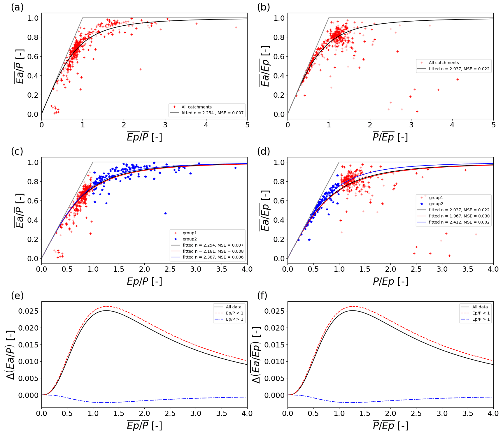
Figure 1 CAMELS dataset plotted in different projections of the Budyko space, with (a) and (c) a projection normalized by precipitation for all catchments and (b), and (d) a projection normalized by potential evaporation. In (c) and (d) the catchments are split into two groups that are either water-limited or energy-limited, with the best fit curve for all catchments in black, the best fit for the group of energy-limited catchments in red and the best fit for the group of water-limited catchments in blue. The differences between the curves in (c) and (d) are shown in (e) for a projection normalized by precipitation, whereas (f) shows the differences between the curves in (c) and (d) for a projection normalized by potential evaporation.

In the next step, the uncertainty in the estimated mean annual actual evaporation due to the different projections was assessed. This was done by selecting one catchment for the prediction of mean annual actual evaporation, whereas the remaining 356 catchments were used to fit the Budyko curve. This was again carried out in a projection based on a wetness index and a dryness index. As both estimates can be considered equally likely, the uncertainty was defined as the relative difference from the mean of the two estimates (i.e., the difference between the estimates equals 2 times the uncertainty). In addition, the predictions were evaluated by the relative error compared with the water balance based observed evaporation. The procedure was repeated for each catchment, leading to uncertainty estimates and relative errors for each catchment. Eventually, predictions were also made by just using the non-contracted side of the framework.

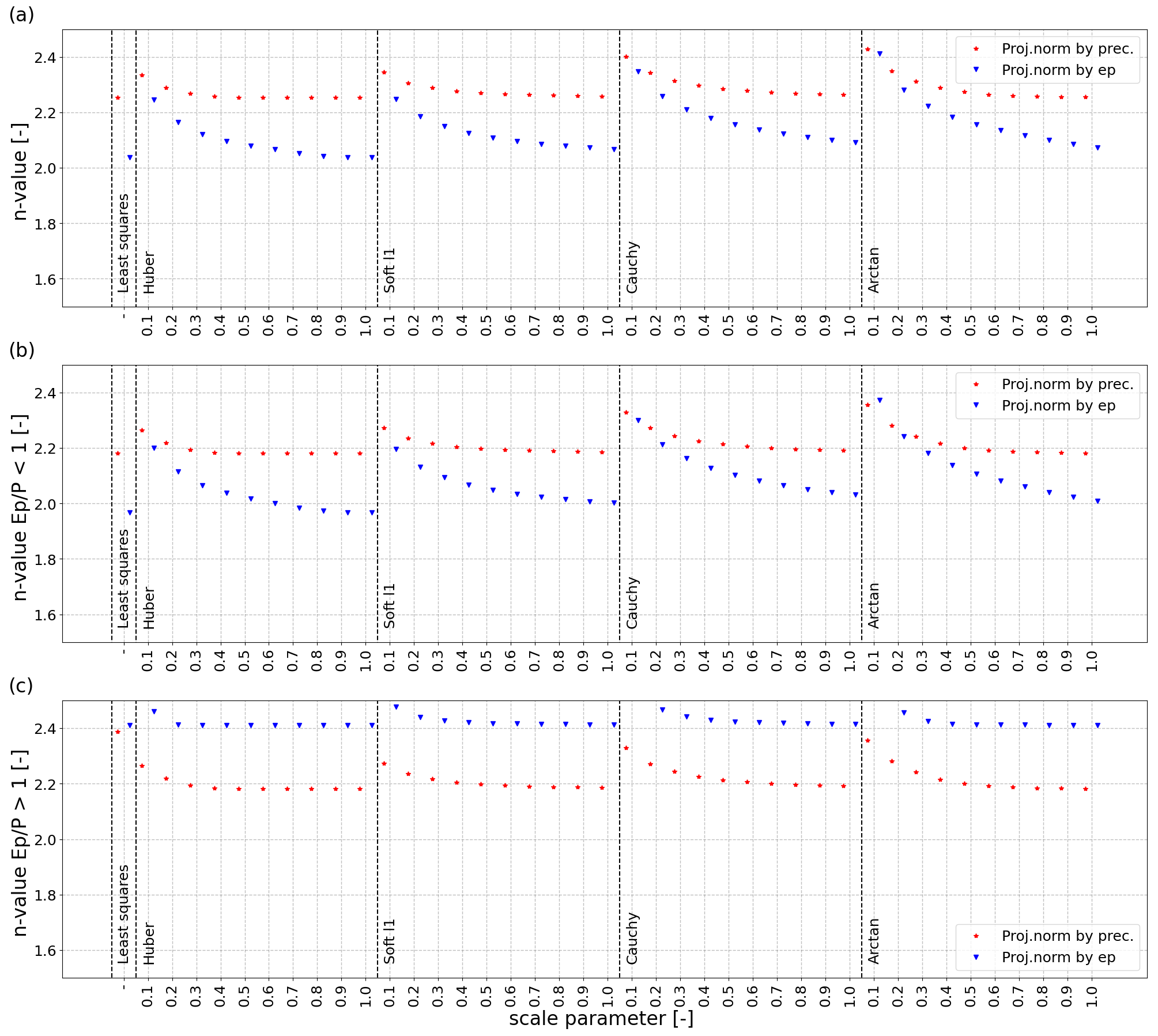
Figure 2 Fitted n values for (a) all catchments, (b) energy-limited catchments and (c) water-limited catchments, for projections that normalized by precipitation (blue) and potential evaporation (red). On the x axis, the different robust regression methods with different scale parameters (separating outliers from the data) are shown.

3 Results and discussion

3.1 Fitting the Budyko curve for different projections

Fitting the selected catchments of the CAMELS dataset to the two different projections led to different values for the n exponent in Eqs. (2) and (3) (Fig. 1a and b, n = 2.254 and n = 2.037, respectively). These n values differed even stronger when the catchments were separated into two groups based on their aridity ($E_{\mathrm{p}}/P>\mathrm{1}$ and $E_{\mathrm{p}}/P\le \mathrm{1}$, respectively, Fig. 1c and d). In particular, for the energy-limited catchments ($E_{\mathrm{p}}/P\le \mathrm{1}$, shown in red), the values changed strongly from an n value of 2.181 in the projection with a dryness index (Fig. 1c) to a value of 1.967 in the projection with a wetness index (Fig. 1d). The differences that occurred when the curves with the two different n values from the two different projections were used in the same projection and subtracted from each other (Fig. 1e and f) also show that especially the curves based on energy-limited catchments strongly deviated ($E_{\mathrm{p}}/P\le \mathrm{1}$, shown in red). In contrast, the curves obtained for water-limited catchments ($E_{\mathrm{p}}/P>\mathrm{1}$, blue) remained more similar, with negligible differences.

The results presented in Fig. 1 also strongly depended on the choice of the method, which was here a linear least-squares fit. Repeating the analysis with more robust methods (see Table 1) led to smaller differences between n values in the two projections, even though differences were still present (Fig. 2a). In particular, the scale parameter C (Eq. 4) that identifies data points as outliers had a strong effect on the resulting n values when set to a larger value. Nevertheless, differences still occurred for small values of this scale parameter, i.e the most stringent values that classify the most data points as outliers, even though these differences became relatively minor. In contrast to what was found with the linear least-squares method, the robust methods resulted in differences in n values for the water-limited catchments (Fig. 2c, differences between blue and red points) that are generally bigger than the differences in n values for the energy-limited catchments (Fig. 2b, differences between blue and red points).

The above results clearly show that the projection used to fit the Budyko curve leads to different n values. Hence, n values that are found by fitting Budyko-type curves include a rather high uncertainty, and the interpretation should be carried out with care. This does not necessarily lead to large issues when n values are considered a characteristic for one single catchment (e.g., Zhang et al., 2001; Donohue et al., 2012; Roderick and Farquhar, 2011), as the equations can be solved analytically when just one data point is considered. However, the two formulations of the curve (Eqs. 2 and 3) stem from the same original equation (Eq. 1), meaning that the definition and value of the parameter should, in principle, not change when projections are changed. For this reason, the different values of the n parameter found here for the different projections express an additional uncertainty due to the choice of projection. When a Budyko curve is fit to multiple catchments and the resulting n values are used for interpretation, this additional uncertainty should be considered.

3.2 Distances to the curve and envelopes

Once a Budyko curve is fit to the data, the distance to this curve is often used as a metric for catchment analysis (e.g., Potter et al., 2005; Yokoo et al., 2008; Williams et al., 2012) and supposed to tell something about the state of the catchment, catchment characteristics or the local climate. However, the distance to the curve strongly changed depending on the projection, and the differences in distances depended on the aridity of the catchments (Fig. 3a). For energy-limited catchments ($E_{\mathrm{p}}/P\le \mathrm{1}$), the distances to the curve were lower for the projection with a wetness index in comparison with the projection with a dryness index (i.e., catchments plot left of the 1:1 line in Fig. 3a), whereas the opposite was true for the water-limited catchments (right of the 1:1 line in Fig. 3a). This was also more generally confirmed when random samples in the Budyko space were used; see Supplement S2. The distances to the physical boundaries are less often used as a metric for catchment analysis, but these changed similarly (Fig. 3b).

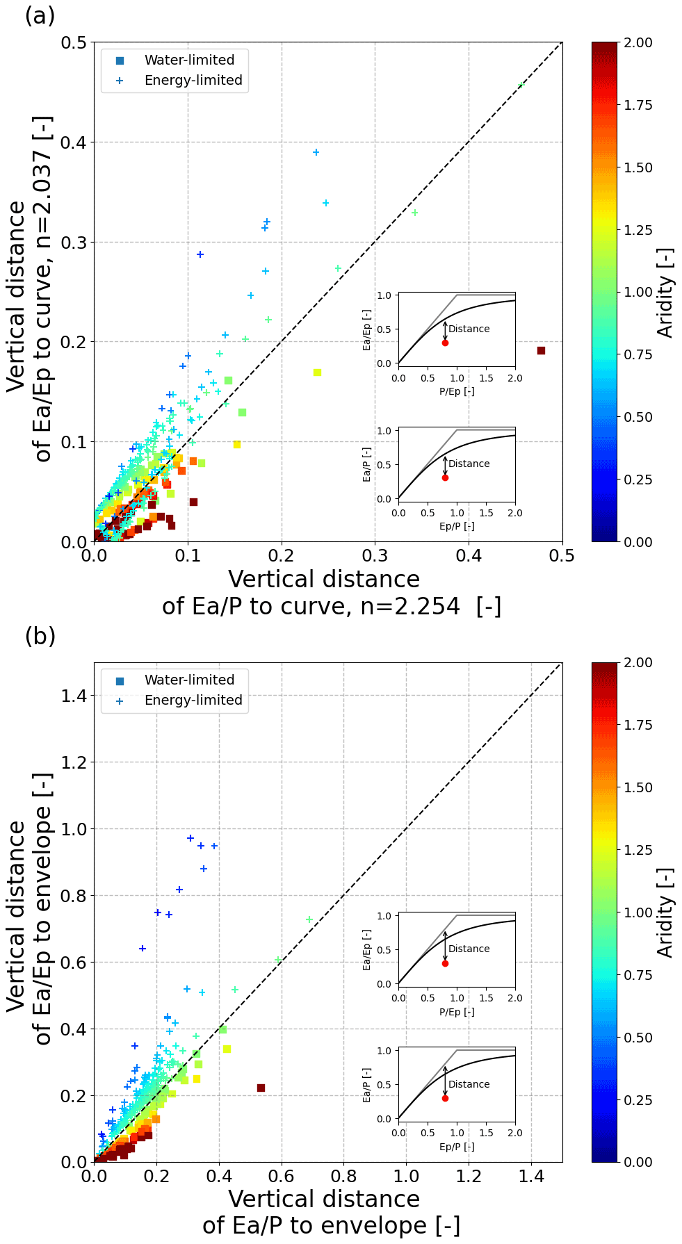
Figure 3 Vertical distances to (a) the envelope of the physical limits of the Budyko framework and (b) vertical distances to the fitted Budyko curve, both for projections normalized by precipitation (x axes) and potential evaporation (y axes). Water-limited catchments ($E_{\mathrm{p}}/P>\mathrm{1}$) are shown by stars, whereas energy-limited catchments are shown by crosses. The color scale indicates the aridity of the catchments.

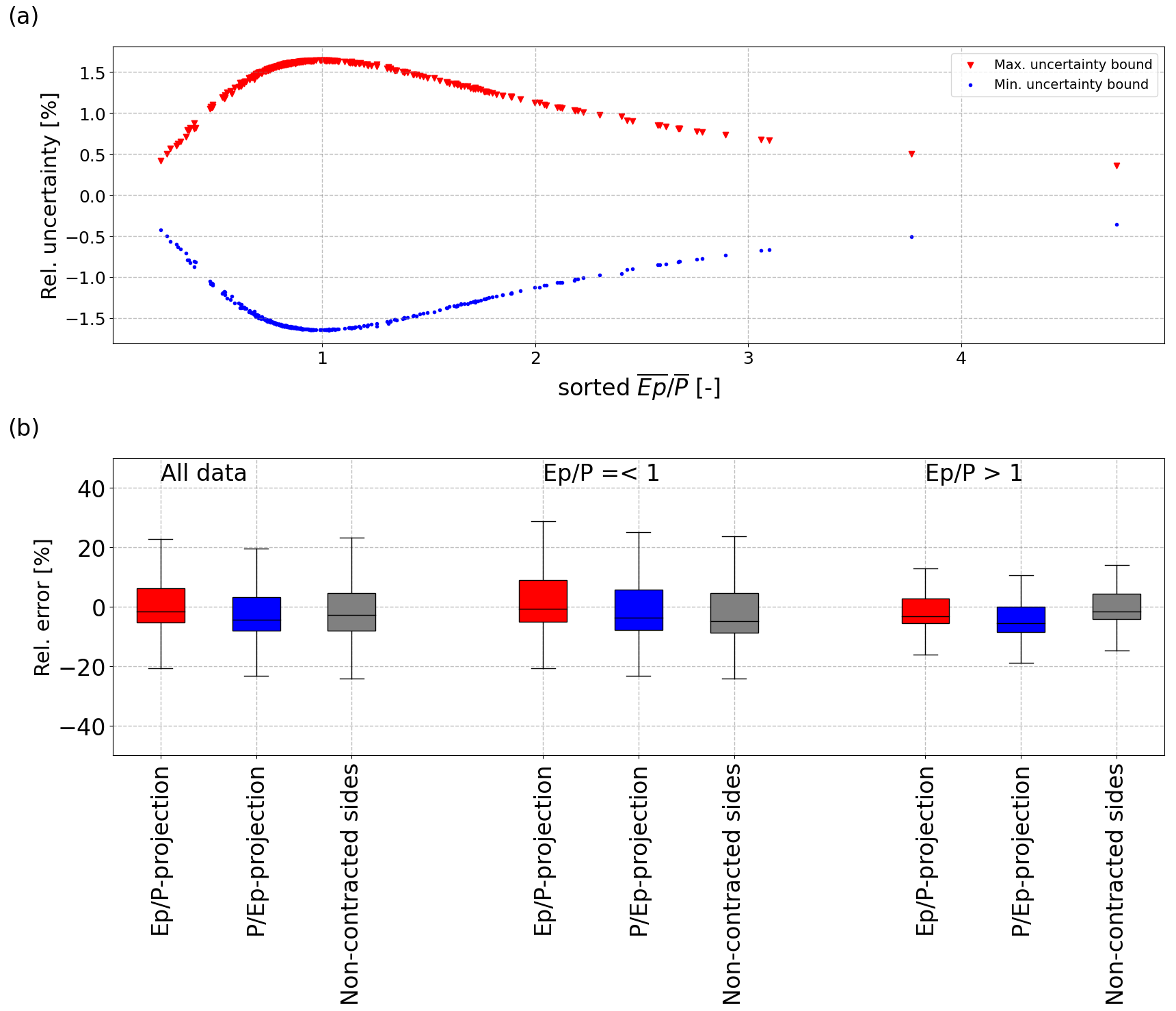
Figure 4 Uncertainty bounds of predicted values of E_a, due to different projections (a). The uncertainty is defined as the relative difference from the expected value of E_a, which is the mean of the predicted values in the two different projections. The relative errors compared with observed (water balance) E_a are shown in (b) for a dryness index projection (red), a wetness index projection (blue) and when only the non-contracted sides of the framework are used (gray). Note that for the blue and red boxplots, the full data are always used to derive the curve, whereas the gray boxplots only used the non-contracted side of the curve. For the gray boxplot with “All data”, the non-contracted sites were used as well; i.e., the curve was fit for catchments with $E_{\mathrm{p}}/P\le \mathrm{1}$ in a wetness index projection and for catchments with $E_{\mathrm{p}}/P>\mathrm{1}$ in a dryness index projection.

These findings imply as well that exchanging projections of the Budyko curve is not as straightforward as it seems and may result in different outcomes. Moreover, different interpretations can be given to these distances, as an increased distance to $E/E_{\mathrm{p}}=\mathrm{1}$ indicates a decreased energy use efficiency, whereas an increased distance to $E/P=\mathrm{1}$ indicates a decreased rain use efficiency by evaporation. In the literature, several studies focus on explaining these distances to the curve (e.g.,  Donohue et al., 2007, 2010; Xiong and Guo, 2012; Fang et al., 2016), rather than the n values, but usually only consider one specific projection. Thus, one needs to be aware that these explanations are only valid for that specific projection because the meaning, as well as the value of these distances, changes for a different projection.

Therefore, also here a consistent use of the framework is needed. As an aridity of 1.0 introduces a clear distinction between under- and overestimating the distances to the curve and envelope in Fig. 3a and b, one may consider using only the side of the curve with $E_{\mathrm{p}}/P>\mathrm{1.0}$ in the dryness index projection or $P/E_{\mathrm{p}}<\mathrm{1.0}$ in the wetness index projection. In this way, the contracted side of the curve is not used, which could lead to errors due to seemingly low absolute deviations that are in relative terms clearly present.

3.3 Uncertainty in predictions

The Budyko framework is often used to predict values of E_a for ungauged catchments, but the uncertainty in predictions of E_a due to the projection used exceeded 1.5 % for catchments with an aridity around 1.0 (Fig. 4a). In addition, the relative error compared with the observed E_a was especially large for energy-limited catchments of the CAMELS dataset ($E_{\mathrm{p}}/P\le \mathrm{1}$, Fig. 4b). However, the differences in the relative errors between the dryness and wetness index based estimates remained rather small (Fig. 4b).

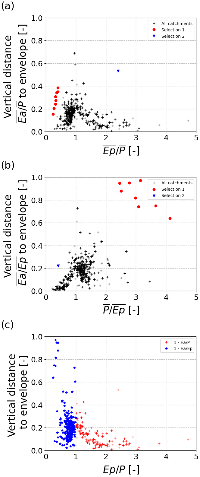
Figure 5 Vertical distances to the envelope for a projection with a dryness index (a) and a wetness index (b), with the same selection in catchments in blue triangles, red dots and black crosses. Distances to the envelope are shown in (c) as a function of the dryness index, with the distances to the non-contracted side in a projection with a dryness index in red (i.e., $E_{\mathrm{p}}/P>\mathrm{1.0}$ with distances $\mathrm{1}-E_{\mathrm{a}}/P$) and the distances to the non-contracted side in a projection with a wetness index in blue (i.e., $P/E_{\mathrm{p}}>\mathrm{1}$ with distances $\mathrm{1}-E_{\mathrm{a}}/E_{\mathrm{p}}$).

The uncertainty in predicted values of E_a due to the choice of projection in the Budyko framework has not received much attention to date. Uncertainty evaluations do exist for the Budyko framework or derivatives thereof (e.g., Yang et al., 2014), but these studies did not consider the influence of different projections. Only Andréassian and Perrin (2012) noted that the chosen projection may lead to ambiguities, especially related to leaky or gaining catchments. Implicitly, others may include the projection-related uncertainty indirectly by defining the curves in a more statistical way (Greve et al., 2015), but we would still argue that the influence of the projection used needs more consideration.

3.4 Influence of outliers

An important cause of the different n values in the different projections are data points that appear as outliers in one projection but not in the other projection. For example, several data points have short vertical distances to the envelope in a dryness index projection but have large distances to the envelope in a wetness index projection and could be considered as outliers (red points in Fig. 5a and b). Vice versa, one data point appears as an outlier in a dryness-index-based projection (blue point in Fig. 5a), but this is not apparent in the other projection (Fig. 5b).

The outliers also influenced the relative errors when the curve was used to predict E_a. The group of catchments identified as outliers in a wetness index projection (i.e., red points in Fig. 5) led to lower n values with a lower curve (see also Fig. 1) and a predicted E_a that is more often underestimated (blue boxes in Fig. 4 shifted downwards). Once only the non-contracted side of the framework was used for predictions, the relative errors became either more negative (for $E_{\mathrm{p}}/P\le \mathrm{1}$) or improved and approached 0 (for $E_{\mathrm{p}}/P>\mathrm{1}$). However, this was merely a result of the absence of the group of outliers (with $E_{\mathrm{p}}/P\le \mathrm{1}$) for the predictions of the catchments with $E_{\mathrm{p}}/P>\mathrm{1}$. Thus, using only the contracted sides of the framework does not necessarily improve predictions of E_a. Nevertheless, we would still argue that plotting the framework in the two projections and, at least, inspecting the non-contracted sides for outliers is a valuable and necessary step in Budyko applications.

4 Conclusions

The Budyko framework was applied to a selection of catchments across the contiguous United States, with two different ways to plot the framework. The first projection used a wetness index, whereas the second projection used a dryness index. First, curves were fit with a standard linear least-squares algorithm, followed by more robust methods afterwards. Distances of individual catchments to the curves and envelopes were determined, in order to assess to effects of the different projections. In the next step, we assessed the uncertainty in predicted values of actual evaporation due to the different projections.

In this way, we gained the following insights:

• The differences in n values due to the projection used were ± 0.2 for this dataset (Fig. 1).

• Robust fitting algorithms reduced the differences in n values in the different projections, but differences were still present (Fig. 2).

• The distances to the curve had a systematic dependence on the projection, with larger differences for the non-contracted side of the framework, i.e., $E_{\mathrm{p}}/P>\mathrm{1}$ for the projection with a dryness index and $P/E_{\mathrm{p}}>\mathrm{1}$ for the projection with a wetness index (Fig. 3).

• The resulting uncertainty in predicted values of E_a, solely due to the projections used, could exceed 1.5 % (Fig. 4).

• Data points can appear as outliers in one projection but not in the other, causing differences in the fitting of the curves (Fig. 5).

These findings show that the projection used needs to be considered carefully. Here, we would like to argue to assess always the non-contracted side of the framework in the two projections. Catchments that seem close to the curve and the limits on the contracted side can easily appear as strong outliers on the non-contracted side of the framework, as the absolute value of the relative errors changes on the x axis on the contracted side (i.e., a 10 % error in $E_{\mathrm{a}}/P$ for $E_{\mathrm{p}}/P=\mathrm{0.5}$ differs in absolute terms for $E_{\mathrm{p}}/P=\mathrm{0.7}$). In contrast, this does not happen when only the non-contracted side is considered. At least, it must be noted and considered that the projection used does lead to differences and adds uncertainty to analyses where Budyko curves are fit to multiple catchments. Studies that use Budyko-type curves should therefore assess whether their results are robust and remain unchanged when the projection is changed.