Low-flow estimation beyond the mean – expectile loss and extreme gradient boosting for spatiotemporal low-flow prediction in Austria

Accurate predictions of seasonal low flows are critical for a number of water management tasks that require inferences about water quality and the ecological status of water bodies. This paper proposes an extreme gradient tree boosting model (XGBoost) for predicting monthly low flow in ungauged catchments. Particular emphasis is placed on the lowest values (in the magnitude of annual low flows and below) by implementing the expectile loss function to the XGBoost model. For this purpose, we test expectile loss functions based on decreasing expectiles (from τ=0.5 to 0.01) that give increasing weight to lower values. These are compared to common loss functions such as mean and median absolute loss. Model optimization and evaluation are conducted using a nested cross-validation (CV) approach that includes recursive feature elimination (RFE) to promote parsimonious models. The methods are tested on a comprehensive dataset of 260 stream gauges in Austria, covering a wide range of low-flow regimes. Our results demonstrate that the expectile loss function can yield high prediction accuracy, but the performance drops sharply for low expectile models. With a median R² of 0.67, the 0.5 expectile yields the best-performing model. The 0.3 and 0.2 perform slightly worse, but still outperform the common median and mean absolute loss functions. All expectile models include some stations with moderate and poor performance that can be attributed to some systematic error, while the seasonal and annual variability is well covered by the models. Results for the prediction of low extremes show an increasing performance in terms of R² for smaller expectiles (0.01, 0.025, 0.05), though leading to the disadvantage of classifying too many extremes for each station. We found that the application of different expectiles leads to a trade-off between overall performance, prediction performance for extremes, and misclassification of extreme low-flow events. Our results show that the 0.1 or 0.2 expectiles perform best with respect to all three criteria. The resulting extreme gradient tree boosting model covers seasonal and annual variability nicely and provides a viable approach for spatiotemporal modeling of a range of hydrological variables representing average conditions and extreme events.

1 Introduction

Prediction of low flow in ungauged basins is a basic requirement for many water management tasks (Smakhtin, 2001). Current estimation procedures aim to estimate some long-term average low-flow characteristics, such as the low-flow quantile Q95 or the 7 d minimum flow, often calculated for a return period of 10 years (Q_7,10) (Salinas et al., 2013). These signatures are either predicted by physically based models (Euser et al., 2013) or statistical methods, such as geostatistical methods (e.g., Castiglioni et al., 2009, 2011; Laaha et al., 2014) and regression-based models (e.g., Laaha and Blöschl, 2006, 2007; Tyralis et al., 2021b; Worland et al., 2018; Ferreira et al., 2021; Laimighofer et al., 2022). Recently, the prediction of seasonal low-flow characteristics has gained increasing interest. Knowing the seasonal (e.g., monthly) distribution of low flows is necessary, e.g., when assessing the water quality or ecological status of water bodies, since low discharges combined with temperature can yield a cascade of hydrochemical processes that vary with the season. Such temporal low-flow characteristics require a new class of models that take temporal signals of predictors into account. Assessment of low flow on a temporal scale is mostly based on empirical characteristics of the modeled hydrograph (e.g., Shrestha et al., 2014; Huang et al., 2017; Lees et al., 2021), with some exceptions where the accuracy of observations below a specific threshold are considered (e.g., Onyutha, 2016). All these approaches show a much higher bias for low flows than for high flows. This is often a consequence of a loss function that emphasizes high flows while giving too little weight to the low-flow events (Staudinger and Seibert, 2014; Staudinger et al., 2011). Although several approaches for modeling monthly or annual streamflow records exist (e.g., Vandewiele and Elias, 1995; Steinschneider et al., 2015; Yang et al., 2017; Ossandón et al., 2022; Pumo et al., 2016; Vicente-Guillén et al., 2012; Cutore et al., 2007; Lima and Lall, 2010; Roksvåg et al., 2020), we noticed a significant research gap in modeling monthly low flow, which to our knowledge has not been investigated to date.

Recently, data-driven models have gained interest for prediction of daily discharge in ungauged basins because of their fast implementation and good prediction performance. These approaches consider a wide range of models, e.g., long short-term memories (LSTMs; Kratzert et al., 2019a, b; Lees et al., 2021) or artificial neural networks (ANNs; Solomatine and Ostfeld, 2008; Dawson and Wilby, 2001; Abrahart et al., 2012). Similar methods are applied to lower temporal resolutions (monthly or annual) of streamflow data, where either parameters of hydrological models are interpolated in space (Yang et al., 2017; Vandewiele and Elias, 1995; Steinschneider et al., 2015), or different statistical methods are applied. Considering the data-driven models, a common approach is to fit independent models to each station (e.g., Shortridge et al., 2016; Parisouj et al., 2020; Chang and Chen, 2018). Such an approach does not seem efficient because spatial correlations of time series at neighboring stations are not considered in parameter estimation. This may lead to spatially inconsistent predictions that also have lower accuracy. Few approaches have been proposed that treat spatiotemporal flow indices in a single, spatiotemporal framework (e.g., Ossandón et al., 2022; Vicente-Guillén et al., 2012; Lima and Lall, 2010; Roksvåg et al., 2020; Pumo et al., 2016; Cutore et al., 2007). These studies either used a combination of deterministic models with kriging (Vicente-Guillén et al., 2012), time-series models (Pumo et al., 2016), or Bayesian hierarchical models (Ossandón et al., 2022; Lima and Lall, 2010; Roksvåg et al., 2020). Surprisingly, little efforts have been made to use statistical learning models for spatiotemporal flow patterns. One exception is Cutore et al. (2007), who tested an ANN model for mean monthly flow and compared it against various regression approaches. They found that a single ANN outperforms methods where regression parameters are interpolated in space, or single multivariable regression.

In this study, we propose to use the extreme gradient boosting model (XGBoost; Chen and He, 2015; Chen and Guestrin, 2016) for modeling spatiotemporal patterns of monthly low flows. The XGBoost model is an ensemble of boosted regression trees and a common model in hydrology (Zounemat-Kermani et al., 2021). Applications range from e.g., modeling water quality (e.g., Lu and Ma, 2020) to estimating groundwater salinity (Sahour et al., 2020). Additionally, XGBoost has shown to be a suitable model for streamflow forecasting (e.g., Yu et al., 2020; Tyralis et al., 2021a; Ni et al., 2020) and its fast implementation is beneficial in our spatiotemporal context. We further explore the use of the expectile loss function as a fitting criterion to give more weights on more extreme flows. Expectile regression (Aigner et al., 1976; Newey and Powell, 1987; Kneib, 2013; Kneib et al., 2021) has rarely been applied in hydrology (Tyralis et al., 2022), but the use of asymmetric weights appear well-suited for estimating flow quantiles beyond the mean (e.g., Toth, 2016). Our model shall also incorporate a variable selection procedure to obtain models that are more parsimonious and easier to interpret.

The objective of our study is to develop such a spatiotemporal low-flow model and to evaluate its performance when predicting at ungauged sites. The following research questions will be addressed: (i) To what extent can spatiotemporal monthly low flow be modeled by one single gradient boosting model? (ii) How does expectile regression perform compared to traditional loss functions (mean absolute error, median absolute error)? (iii) How accurate are low extremes modeled by different expectiles? (iv) Which spatial and spatiotemporal variables are used for different expectiles? Our analysis will be performed on a comprehensive Austrian streamflow dataset representing a range of seasonal low-flow regimes.

2 Data and methods

2.1 Data

2.1.1 Hydrological data

Our study area covers 260 gauging stations in Austria with different low-flow seasonality. The dataset was already used in a wide range of studies (e.g., Laaha and Blöschl, 2006, 2007; Laaha et al., 2014; Laimighofer et al., 2022). Some stations included in previous studies had to be discarded as the gauging stations were removed, relocated, or the data included too many missing values. The hydrological data are available from the Hydrographic Service of Austria (HZB) and all stations have a continuous daily streamflow record from 1982 to 2018. From these data, we calculated the monthly low-flow index series for each station, using the monthly Q95 $\left(P\right(Q>Q\mathrm{95})=\mathrm{0.95})$ to characterize the low-flow regime (Fig. 1). The index is very similar to the monthly 7 d minimum flow MM(7), which has been used in an earlier study to assess the timing of low-flow events on a pan-European scale (Laaha et al., 2017). For one station, a monthly value had to be inserted using smoothed empirical orthogonal functions (Lindström et al., 2014) to preserve the station despite single missing values in the daily discharge record. The monthly Q95 was standardized by the catchment area, resulting in the monthly specific low-flow (q95) time series (l s⁻¹ km⁻²) for each station, which constitutes the target variable of our study. The monthly q95 series were further transformed by the square root to give less weight to the high low flows, according to preliminary evaluations. Finally, model evaluation was performed using the predictions after transforming back to the original scale.

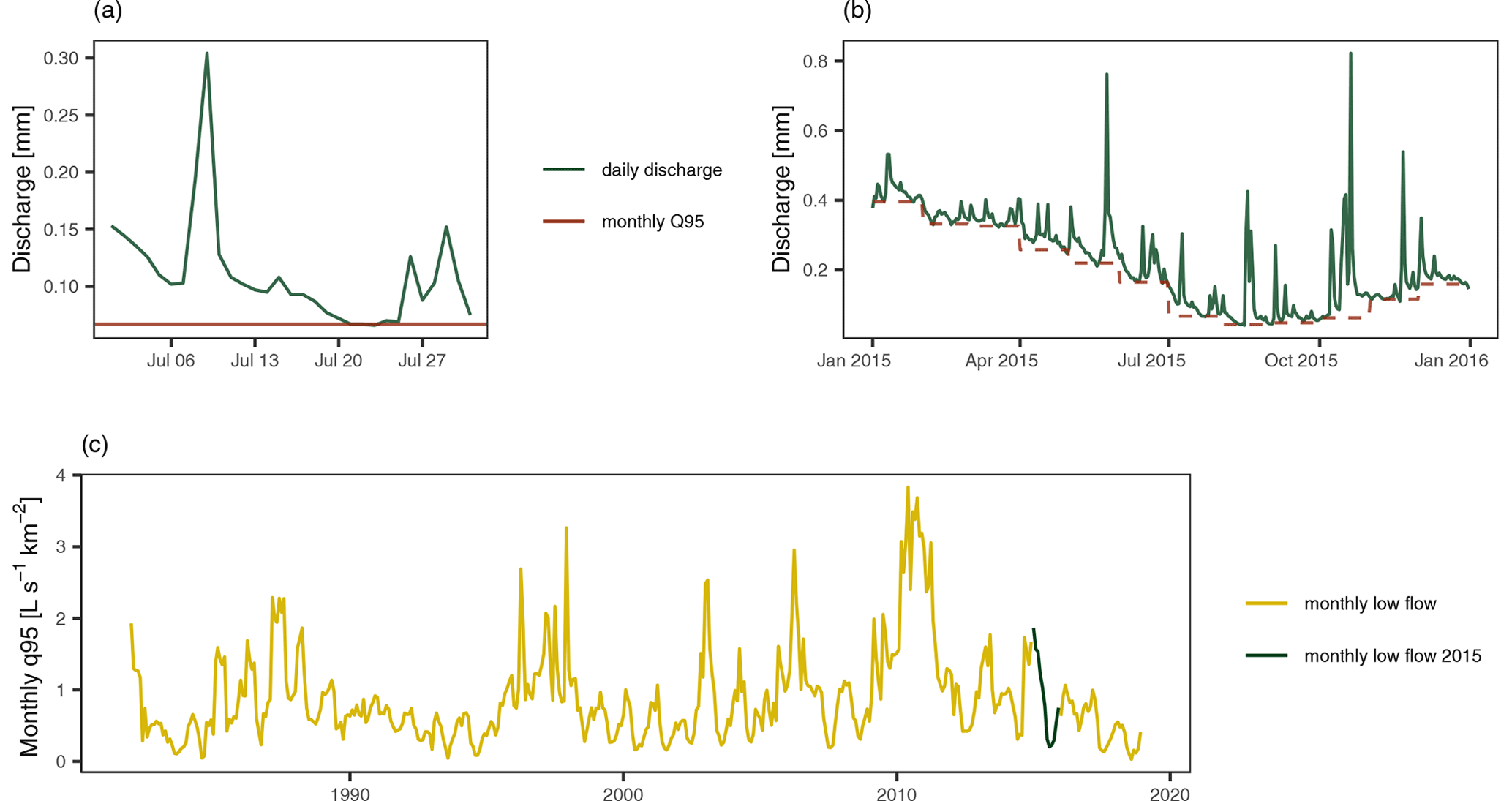
Figure 1 Example of the calculation of the monthly q95 time series for the gauging station Hollenstein in lower Austria. Panel (a) shows the daily discharge in July 2015, (b) represents the monthly q95 and daily discharge for the full year of 2015, and (c) displays the full monthly q95 time series for the station.

Additionally, we used specific discharge quantiles with 0.95, 0.98, and 0.99 exceedance probability from the daily discharge series (q95_d, q98_d, q99_d) to identify extreme events in our monthly series. This threshold selection procedure classifies about 11 % (q95_d), 5 % (q98_d), and 3 % (q99_d) of observations at each station as extreme low-flow events.

2.1.2 Predictor variables

Spatiotemporal modeling requires predictor variables, of which two types can be distinguished. The first type consists of climate and catchment characteristics representing the long-term average hydrological conditions. This type corresponds to typical predictors in low-flow regionalization models such as regional regression approaches (Laaha et al., 2013). The second type of predictors consists of spatiotemporal covariates that capture the climate drivers of low-flow generation. These dynamic predictors are needed to extend the regional model with a temporal dimension so that spatiotemporal patterns of low flow can be represented. The former type will be referred to as static predictors, the latter as spatiotemporal covariates throughout the paper.

Table 1 Descriptions of static predictors used in the study, structured in topological, land-use, geological, and meteorological characteristics. Abbreviations are further used in plots. Precipitation, climatic water balance, potential evapotranspiration, aridity index, snowmelt, and temperature variables are used on an annual and a summer/winter half-year basis. These different accumulation periods are indicated in the subscript: no subscript for annual characteristics (e.g., P), win for winter (e.g., P_win), sum for summer (e.g., P_sum).

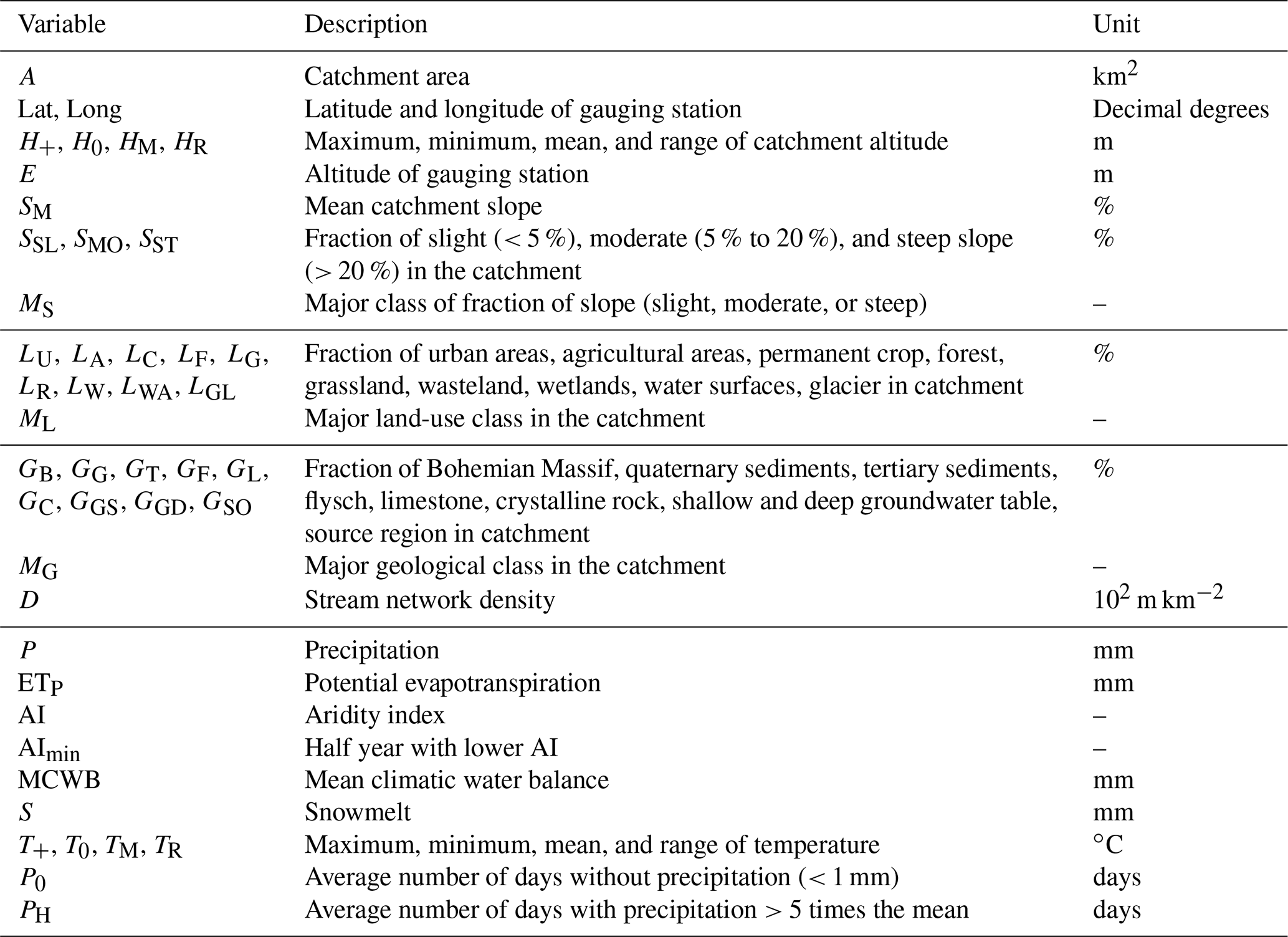
For the static predictors, we used a set of climate and catchment characteristics of precedent rationalization studies in Austria (e.g., Laaha and Blöschl, 2006; Laimighofer et al., 2022). They consist of topological and land-use variables, geological classes, and long-term average meteorological characteristics such as precipitation (P), mean climatic water balance (MCWB), and others (Table 1). All these variables are aggregated on an annual basis (no subscript: e.g., P, MCWB), for the summer half-year from April to September (e.g., P_sum, MCWB_sum), and for the winter half-year from October to March (e.g., P_win, MCWP_win). For more details about their calculation, see Laimighofer et al. (2022) and Laaha and Blöschl (2006).

For spatiotemporal covariates, the initial choice of the variables is also important, as it can affect model performance and interpretability of results. In a preliminary assessment (not shown in this paper), we tested several combinations of spatiotemporal covariates, including monthly precipitation, climatic water balance (CWB), temperature, snowmelt, solid precipitation, or soil moisture characteristics. All these combinations were tested by a nested 10-fold cross validation (CV; see Sect. 2.2.3 for more detail) and compared to a range of error metrics (Sect. 2.2.4). The results showed that the monthly CWB calculated as the difference between monthly precipitation and potential evapotranspiration performs equivalently to the combination of its components provided as individual model terms. Since our study focuses more on a methodological assessment, we decided to only include the CWB as a spatiotemporal predictor for the sake of simplicity. Note that the CWB enters the model as a static variable (MCWB) and as a spatiotemporal covariate on a monthly basis (CWB). The former serves as an intercept in the model, the latter as a temporal signal that determines the monthly low-flow series.

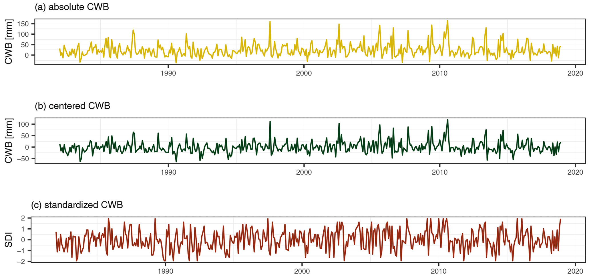
Figure 2 Example of the transformations of the climate water balance (CWB) with no lag at station Hollenstein. Panel (a) shows the absolute values of the CWB. Panel (b) represents the CWB centered for each month and (c) is a computation of a non-parametric standardized drought index (SDI) for each month.

Table 2 Description of the different lags and transformations for the CWB. Center means centering per station and month and the standardized drought index (SDI) is transforming the CWB to an SDI per station and month.

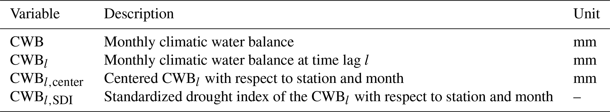
The monthly CWB series are further coded as time lags (l) from 1 to 12 months (CWB_l) before each value in the target series. These lags are assumed to represent antecedent conditions in low-flow generation. In addition to using “raw” CWB values, the CWB was additionally transformed in order to test whether standardization has an effect on the performance of the predictor. First, each spatiotemporal variable (CWB, CWB_l) is centered by month (m) and station (s) via ${\mathrm{CWB}}_{\mathrm{center},s,m}={\mathrm{CWB}}_{s,m}-{\stackrel{\mathrm{‾}}{\mathrm{CWB}}}_{s,m}$, where CWB_s,m is the monthly climatic water balance at a station, and ${\stackrel{\mathrm{‾}}{\mathrm{CWB}}}_{s,m}$ its monthly mean. Second, we transform the climatic water balance (CWB, CWB_l) to a non-parametric standardized drought index (SDI), similar to the SPEI (Beguería et al., 2014). Instead of fitting a parametric distribution, we estimate the empirical probability of the CWB_s,m. The empirical probabilities are then transformed to quantiles of a standard normal distribution. A visualization of these two transformations is given in Fig. 2 and a short overview of the variables in Table 2. These two transformations are highly correlated to the initial CWB, but can provide additional information for our model. All these lags and transformations are used simultaneously as input variables for our model, resulting in 39 spatiotemporal predictor variables.

Apart from the static predictions and the spatiotemporal covariates, some variables were added to capture the temporal periodicity. The numeric variable of the month ($m=\mathrm{1},\mathrm{2},\mathrm{\dots },\mathrm{12}$), was converted to a categorical variable and additionally transformed to a sine and cosine curve so that their two-dimensional overlay gives a representation of the annual circle. In addition, the year was added as a numeric variable, and finally a cumulative sum of months ($m_{\mathrm{cum}}=\mathrm{1},\mathrm{2},\mathrm{\dots }\mathrm{444}$) was added in order to represent long-term trends of low flows. In total, this results in an initial set of 116 predictor variables that are used for the variable selection procedure.

2.2 Methods

2.2.1 Extreme gradient tree boosting

Extreme gradient tree boosting (Chen and He, 2015; Chen and Guestrin, 2016) is a fast implementation of gradient tree boosting (Friedman, 2001) and based on the general boosting algorithm (Friedman et al., 2000). The method is robust to overfitting and beneficial when predictors are collinear. Gradient tree boosting consists of an ensemble of additive trees that are each fitted by a greedy algorithm to minimize a predefined loss function. Let y​​​​​​​ be a vector of our response variable (monthly specific low flow q95) of length $n=s\cdot t$, where s is the number of stations and t the length of each individual time series per station, and index i referring to its ith element. Further, let X be our predictor matrix with n×p elements, wherein p is the number of predictor variables. We can then write the regression equation as

$$\begin{array}{}\text{(1)}& {\widehat{y}}_i=\sum _{k=\mathrm{1}}^K{f}_k\left(X_i\right),f_k\in F,\end{array}$$

where $f_k(k=\mathrm{1},\mathrm{\dots },K)$ is the ensemble of regression trees, and K the number of trees used. The regression trees are fitted in an additive manner, where an objective function L^k is minimized:

$$\begin{array}{}\text{(2)}& L^k=\sum _{i=\mathrm{1}}^{n}L\left(y_i,{\widehat{y}}_i^{k-\mathrm{1}}+\mathit{\eta }{f}_k\left(x_i\right)\right)+\mathrm{\Omega }\left(f_k\right).\end{array}$$

The kth iteration loss is denoted as L^k, ${\widehat{y}}_i^{k-\mathrm{1}}$ is the prediction of the regression tree in the previous iteration, f_k is the tree that most improves our model considering the predefined loss function, Ω(f_k) is an additional penalization parameter for the complexity of the model and η is a shrinkage parameter. The shrinkage parameter η is set to 0.1, where a small value of η minimizes the risk of overfitting and the possibility of finding only local minima. To reduce the computational burden, we tuned only the following hyperparameters for the final predictions: the maximum depth (the final XGBoost was optimized for a sequence from 6–8) of each additive tree, subsampling of predictor columns (0.25–1), which only uses a fraction of all predictors to search for the optimal split and subsampling of the observations (0.5–1), equivalent to random forests. Subsampling of the observations and the predictor variables is used to decorrelate the trees. The maximum depth can be described as the order of interaction used in the model. Finally, we introduced an early stopping rule for the boosting iterations, where the algorithm stops when the error does not decrease for K=50 iterations. The range of hyperparameters was set based on experience with the XGBoost model and our individual dataset. The final XGBoost model was optimized in a 10-fold CV by using all parameter combinations and tuning the number of boosting iterations (number of trees). A detailed description of our validation scheme is given in Sect. 2.2.3).

2.2.2 Loss function

One crucial point in our study is the application of a suitable loss function. The loss function has to be a twice differentiable convex function. Since our main aim is to model the low flows in the range of annual minima corresponding to the lower tail of the monthly q95 series, we propose using the expectile loss ($L_{\mathrm{EL}}^{\mathit{\tau }}$) for model fitting. Expectile regression (Aigner et al., 1976; Newey and Powell, 1987) is a squared variant of quantile regression (Koenker and Bassett, 1978), where the absolute deviations are substituted by the squared deviations (Kneib, 2013). Expectile regression was already implemented in a boosting framework (Sobotka and Kneib, 2012) and the resulting expectile loss can be defined as follows:

$$\begin{array}{}\text{(3)}& L_{\mathrm{EL},i}^{\mathit{\tau }}=\left\{\begin{array}{ll}\mathit{\tau }\cdot {\left(y_i-{\widehat{y}}_i\right)}^{\mathrm{2}},& \left(y_i-{\widehat{y}}_i\right)\ge \mathrm{0}\\ (\mathrm{1}-\mathit{\tau })\cdot {\left(y_i-{\widehat{y}}_i\right)}^{\mathrm{2}},& \left(y_i-{\widehat{y}}_i\right)<\mathrm{0},\end{array}\right.\end{array}$$

where $L_{\mathrm{EL},i}^{\mathit{\tau }}$ is summed up to $L_{\mathrm{EL}}^{\mathit{\tau }}$ ($L_{\mathrm{EL}}^{\mathit{\tau }}={\sum }_{i=\mathrm{1}}^n{L}_{\mathrm{EL},i}^{\mathit{\tau }}$) for minimizing the error over all observations. If τ=0.5, the expectile loss is a scaled variant of a squared loss function ($L_{\mathrm{squared}}={\sum }_{i=\mathrm{1}}^n(y_i-{\widehat{y}}_i{)}^{\mathrm{2}}$) resulting in a least squares regression. Figure 3 shows that altering τ leads to an asymmetric weighting of the squared loss, where smaller τ give more emphasis on negative residuals. Expectiles cannot directly be interpreted as a flow quantile, as this would be possible for quantile regression, but studies show that using transfer functions can do this very accurately (Waltrup et al., 2015) and differences mainly arise in the tail of the distribution. Estimating a full distribution of τ values is not a very practical approach for our large dataset. Therefore, we will assess a sequence of τ values (τ=0.01, 0.025, 0.05, 0.1, 0.2, 0.3) and the special case of a least squares regression (τ=0.5). Within this sequence, the τ values of 0.1,0.05, and 0.025 give good approximations of our three thresholds: q95_d, q98_d, and q99_d. Finally, we will compare the expectile loss function to the absolute loss (Fig. 3):

$$\begin{array}{}\text{(4)}& L_{\mathrm{abs},i}=|y_i-{\widehat{y}}_i|.\end{array}$$

In case of the absolute loss, the mean absolute error will be minimized by the mean $\left(\mathrm{MAE}=\frac{{\sum }_{i=\mathrm{1}}^n{L}_{\mathrm{abs},i}}{n}\right)$, and in case of the median absolute loss by the median ($\mathrm{MDAE}=\mathrm{median}\left(L_{\mathrm{abs},i}\right)$). In both cases, the second derivative is approximated by a vector of 1 s.

Figure 3 Comparison of different loss functions. Expectile loss functions are shown for various τ parameters and the absolute loss function.

2.2.3 Variable selection and validation scheme

Model evaluation is performed by a nested 10-fold CV (Varmuza and Filzmoser, 2016). A nested CV contains two loops: an inner loop which is used for tuning of hyperparameters and variable selection and an outer loop for evaluating the predictive performance of the models (Laimighofer et al., 2022). In each inner loop, we include a variable selection by recursive feature elimination (RFE; Granitto et al., 2006). The RFE algorithm consists of an initial variable ranking and a backward variable selection. The initial variable ranking is computed by using the XGBoost algorithm with 500 boosting iterations and default hyperparameters (maximum depth = 8, subsample = 1, fraction of p = 0.5). The variables are ranked after their additive gain in minimizing the loss function over the 500 boosting steps. For a more robust approach, the initial variable ranking is averaged over 25 bootstrap samples. The gain of each variable for the final variable ranking is the ratio of the individual additive gain to the total gain over all variables. In a next step, we are fitting an XGBoost model to a sequence from 5 to the maximum number of variables (p), but only with a step length of 5 to reduce the computational burden. For each number of variable, the error is calculated and averaged over all 10-fold CV runs of the inner loop. The number of variables are then determined by using a threshold of 1.05 times the minimum error to produce parsimonious models. This approach yields models with fewer variables at only a small loss in predictive accuracy. Our method ensures that predictors are only selected when they increase the predictive performance of the model. In addition, the outer loop evaluates the predictive performance at ungauged sites independently of model fitting. The applied method is fully described in Laimighofer et al. (2022) and to increase clarity we added a visual explanation of the full CV procedure (Fig. 4).

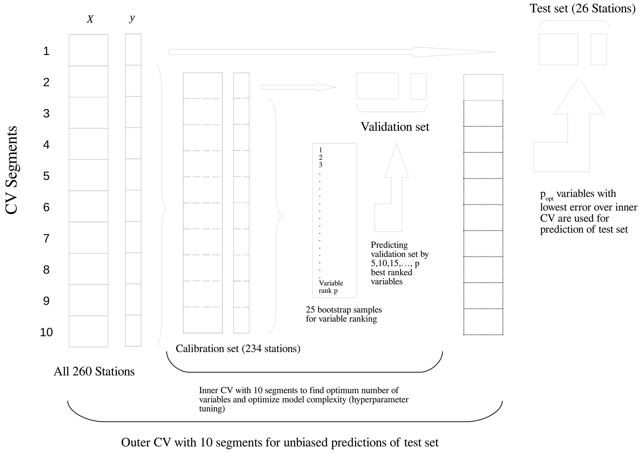
Figure 4 The nested cross-validation (CV) procedure as adapted from the double CV-scheme of Varmuza and Filzmoser (2016).

2.2.4 Model evaluation

Model evaluation is performed by several error metrics. First, we quantify the overall performance of the model by means of four error metrics, the median absolute error (MDAE), the mean absolute error (MAE), the root mean squared error (RMSE):

$$\begin{array}{}\text{(5)}& \mathrm{RMSE}=\sqrt{\mathrm{1}/N\sum _{i=\mathrm{1}}^N{\left(y_i-{\widehat{y}}_i\right)}^{\mathrm{2}}},\end{array}$$

and the coefficient of determination R², which – by our definition – is the same as the Nash–Sutcliffe efficiency (NSE) (Blöschl et al., 2013):

$$\begin{array}{}\text{(6)}& R^{\mathrm{2}}=\mathrm{1}-{\displaystyle \frac{{\sum }_{i=\mathrm{1}}^N{\left(y_i-\widehat{y}\right)}^{\mathrm{2}}}{{\sum }_{i=\mathrm{1}}^N{\left(y_i-\stackrel{\mathrm{‾}}{y}\right)}^{\mathrm{2}}}}.\end{array}$$

All measures are based on CV and therefore are indicators of the predictive performance when estimating at ungauged sites.

Second, we assess the predictive performance for individual stations by calculating the R² for each station separately. The station-by-station performance is summarized by the distribution and the median R² over all stations, which will be referred to as $R_{\mathrm{med}}^{\mathrm{2}}$ throughout the paper.

For a more comprehensive evaluation of the performance, we perform a decomposition of the station-wise prediction errors on different time scales. The purpose is to assess the extent to which the model errors occur at the annual, seasonal, and monthly level, and which part of the error is due to a systematic error (i.e., bias). This will allow us to get insight into structural strength and weaknesses of the models. This decomposition is done by a three-way ANOVA, which was applied by e.g., Parajka et al. (2016) for assessing uncertainty contributions of climate projections. The basic linear model for our ANOVA can be defined as follows:

$$\begin{array}{}\text{(7)}& y_{m,\mathrm{yr}}-{\widehat{y}}_{m,\mathrm{yr}}=\mathit{\mu }+{\mathit{\alpha }}_m+{\mathit{\beta }}_{\mathrm{yr}}+{\mathit{ϵ}}_{m,\mathrm{yr}},\end{array}$$

where the left-hand side (predictand) are the prediction errors of a model at a single station. These are decomposed into the terms μ representing the mean error (i.e., bias), α_m the seasonal effects ($m=\mathrm{1},\mathrm{2},\mathrm{\dots },\mathrm{12}$), β_yr the mean annual effects ($yr=\mathrm{1},\mathrm{2},\mathrm{\dots },\mathrm{37}$), and the residual term ϵ_m,yr corresponding to the model errors at the monthly level. Note that μ is not a classical intercept but enters as a constant factor (coded as a vector of 1 s) which allows the bias to be considered as a separate effect in the error decomposition. In the ANOVA framework, the total variance of the prediction errors is characterized by the total sum of squares SS_T, and is decomposed into additive variance components of individual effects:

$$\begin{array}{}\text{(8)}& {\mathrm{SS}}_{\mathrm{T}}={\mathrm{SS}}_{\mathrm{bias}}+{\mathrm{SS}}_{\mathrm{season}}+{\mathrm{SS}}_{\mathrm{year}}+{\mathrm{SS}}_{\mathrm{E}}.\end{array}$$

The variance contributions of each term are estimated by the measure ω², which is an analogue to the coefficient of determination. The measure ω² of, e.g., the seasonal effect is defined as:

$$\begin{array}{}\text{(9)}& {\mathit{\omega }}_{\mathrm{season}}^{\mathrm{2}}={\displaystyle \frac{{\mathrm{SS}}_{\mathrm{season}}-{\mathrm{df}}_{\mathrm{season}}\cdot {\mathrm{MS}}_{\mathrm{E}}}{{\mathrm{SS}}_{\mathrm{T}}-{\mathrm{MS}}_{\mathrm{E}}}},\end{array}$$

where df_season are the degrees of freedom (i.e., number of factor levels −1), and ${\mathrm{MS}}_{\mathrm{E}}={\mathrm{SS}}_{\mathrm{E}}/{\mathrm{df}}_{\mathrm{E}}$ the residual mean squared error, which can be seen from the ANOVA table. The contribution of the mean annual effect (${\mathit{\omega }}_{\mathrm{year}}^{\mathrm{2}}$) and the fraction of the bias (${\mathit{\omega }}_{\mathrm{bias}}^{\mathrm{2}}$) can be determined analogously and a more detailed description can be found in Parajka et al. (2016). Finally, the residual term ${\mathit{\omega }}_{\mathrm{E}}^{\mathrm{2}}$ can be calculated as follows:

$$\begin{array}{}\text{(10)}& {\mathit{\omega }}_{\mathrm{E}}^{\mathrm{2}}=\mathrm{1}-{\mathit{\omega }}_{\mathrm{season}}^{\mathrm{2}}-{\mathit{\omega }}_{\mathrm{year}}^{\mathrm{2}}-{\mathit{\omega }}_{\mathrm{bias}}^{\mathrm{2}}.\end{array}$$

The last part of our model evaluation specifically emphasizes the extreme low flows. This is assessed by three performance metrics. First, we filter the observations at each station by a specific quantile and calculate the overall R² based on the residuals of the filtered cases. Second, we calculate the relative expectile error (EL_τ) at each station:

$$\begin{array}{}\text{(11)}& {\mathrm{EL}}_{\mathit{\tau }}=\mathrm{1}-{\displaystyle \frac{L_{\mathrm{EL}}^{\mathit{\tau }}\left(y_i,{\widehat{y}}_i\right)}{L_{\mathrm{EL}}^{\mathit{\tau }}\left(y_i,q(y,\mathit{\tau })\right)}}.\end{array}$$

The error metric is defined in analogy to the expectile loss function to give more weight to the fraction of τ lowest values. The denominator ($L_{\mathrm{EL}}^{\mathit{\tau }}$) is the naive estimate for each station. For this purpose, we are using the τ-quantile of the observations (q(y,τ)) as a simple prediction at the specific station, assuming that quantiles and expectiles give similar estimates. The numerator, on the other hand, is the expectile error ($L_{\mathrm{EL}}^{\mathit{\tau }}$) for the predictions of our model. Similar to the R², the EL_τ is bounded at a maximum of 1, representing perfect model fit. Values below 0 indicate that the naive prediction of the τ-quantile would result in a better prediction than our model. One advantage of this metric is that it is based on the full data, but gives more weight to the values below our selected τ.

Finally, we want to capture the model ability of classifying extreme low-flow events. For this purpose, the specific low-flow quantiles q95_d, q98_d, and q99_d are calculated from the daily discharge records and used as thresholds for identifying drought events in the monthly low-flow series. Based on these thresholds, the drought/no drought cases of observed and predicted monthly time series are binary coded, and we calculate the hit score (H_S) and the precision (P_rec) for evaluating the performance at each station. The hit score (also termed recall, sensitivity, or true positive rate) is calculated by

$$\begin{array}{}\text{(12)}& H_{\mathrm{S}}={\mathrm{ET}}_{\mathrm{pred}}/E_{\mathrm{obs}},\end{array}$$

where E_obs is the number of low-flow events in the original data and ET_pred is the number of low-flow events correctly classified by the predictions. The precision is computed as follows:

$$\begin{array}{}\text{(13)}& P_{\mathrm{rec}}={\displaystyle \frac{{\mathrm{ET}}_{\mathrm{pred}}}{{\mathrm{ET}}_{\mathrm{pred}}+{\mathrm{EF}}_{\mathrm{pred}}}},\end{array}$$

where EF_pred is the number of low flows falsely predicted by each monthly time series.

The data analysis was performed in R (R Core Team, 2021) and we want to acknowledge the use of the following packages: XGBoost (Chen et al., 2021), dplyr (Wickham et al., 2021), purrr (Henry and Wickham, 2020), tidyr (Wickham, 2021), ggplot2 (Wickham, 2016), caret (Kuhn, 2021), glmnet (Friedman et al., 2010), tidyselect (Henry and Wickham, 2021), tibble (Müller and Wickham, 2021), receipes (Kuhn and Wickham, 2021), ggthemes (Arnold, 2021), lubridate (Grolemund and Wickham, 2011), wesanderson (Ram and Wickham, 2018).

3 Results

3.1 Global model performance

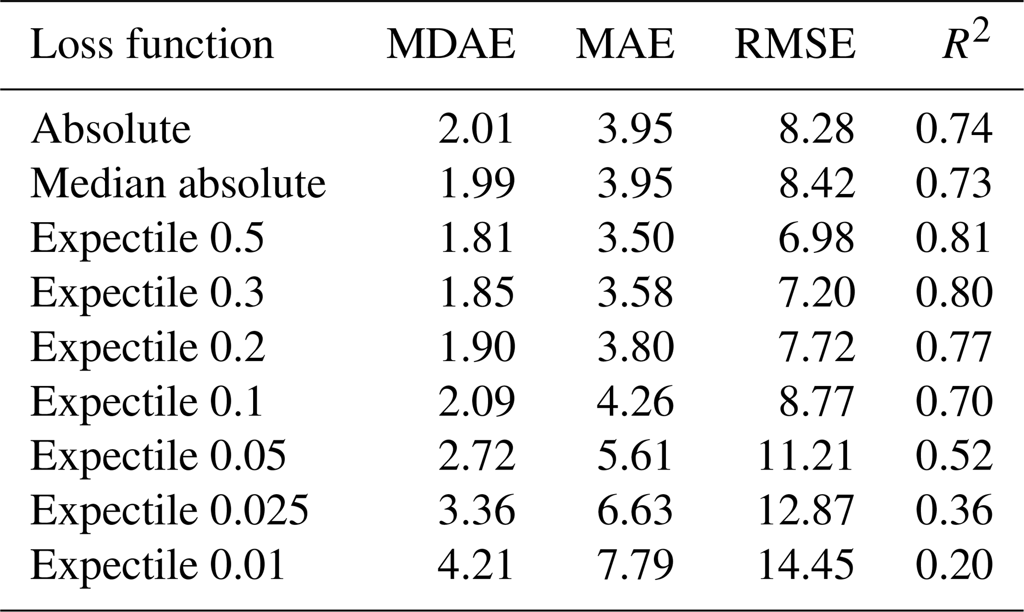
Table 3 presents the results for the overall performance of our spatiotemporal model. Generally, most loss functions show a good overall performance. The 0.5 expectile yields the best R² of 0.81, which is substantially higher than 0.73 for the median absolute loss and 0.74 for the mean absolute loss. Regarding the MDAE, which gives more focus on low values, there is no change in the overall ranking of methods, with a MDAE of 1.81 for the 0.5 expectile, 1.99 for the median absolute loss, and 2.01 for the mean absolute loss. Regarding the results of the expectiles with τ smaller than 0.5, we can identify a decreasing performance towards smaller expectiles over all performance metrics. The R² is stable until the 0.3 expectile and then suddenly drops from 0.8 (0.3 expectile) to 0.2 for the 0.01 expectile. A similar loss in performance can also be observed with the MDAE, MAE, or RMSE. Expectiles below 0.05 show an insufficient performance on these global error metrics. For example, the RMSE of the 0.01 expectile is twice as high as the RMSE of the 0.5 expectile. Nevertheless, expectiles such as 0.2 and 0.3 show better overall metrics than the median absolute loss and the absolute loss, and even the 0.1 expectile demonstrates only a somewhat lower R² of 0.7.

Table 3 Overview of the error metrics for all loss functions. Shown are the MDAE, MAE, RMSE, and R², all representing the overall predictive performance of the model for the study area.

3.2 Station-by-station performance

A more detailed examination of our results is realized by analyzing the performance per station. Table 4 gives an overview of the results and Fig. 5 shows the empirical cumulative distribution of the station-specific R². From the graphs, the 0.5, 0.3, and 0.2 expectiles outperform the other models across all stations. The 0.5 expectile has the highest $R_{\mathrm{med}}^{\mathrm{2}}$ (0.67) and shows a far better performance than the median absolute loss (0.57) and the mean absolute loss (0.58). This generally good performance is further underlined by the finding that only 26 % of the stations have a R² below 0.5 for the 0.5 expectile. In contrast, for the mean and median absolute losses, about 40 % of the stations yield a R² below 0.5. For the expectiles lower than 0.5, we can identify a decrease of the $R_{\mathrm{med}}^{\mathrm{2}}$, from 0.65 for the 0.3 expectile to 0.14 for the 0.05 expectile. Generally, low expectiles (0.01, 0.025, 0.05) yield a high number of inadequate models, where almost 90 % of the stations obtain a R² below 0.5 for the 0.05 expectile. In case of the 0.01 expectile, no station has a R² greater than 0.5. However, the 0.2 and 0.3 expectiles still yield a higher $R_{\mathrm{med}}^{\mathrm{2}}$ of 0.65 and 0.6, compared to the mean absolute loss (0.58) and median absolute loss (0.57). Further, the fraction of stations with a weak performance (R²<0.5) is also lower for the 0.2 and 0.3 expectiles as shown in Table 4. These findings suggest, in response to our first research question, that a single model can provide very accurate results for most stations (0.5, 0.3, 0.2 expectiles), but 26 % to 36 % of the stations have inadequate performance. The origin of these errors will be analyzed in more depth in the subsequent section. As the results of the mean and the median absolute loss could not compete with the performance of the 0.2, 0.3, and 0.5 expectiles, we will not further include these two loss functions in our analysis.

Table 4 Performance per station summarized by the median R² over all stations ($R_{\mathrm{med}}^{\mathrm{2}}$) and the fractions of stations with an R² below 0.5.

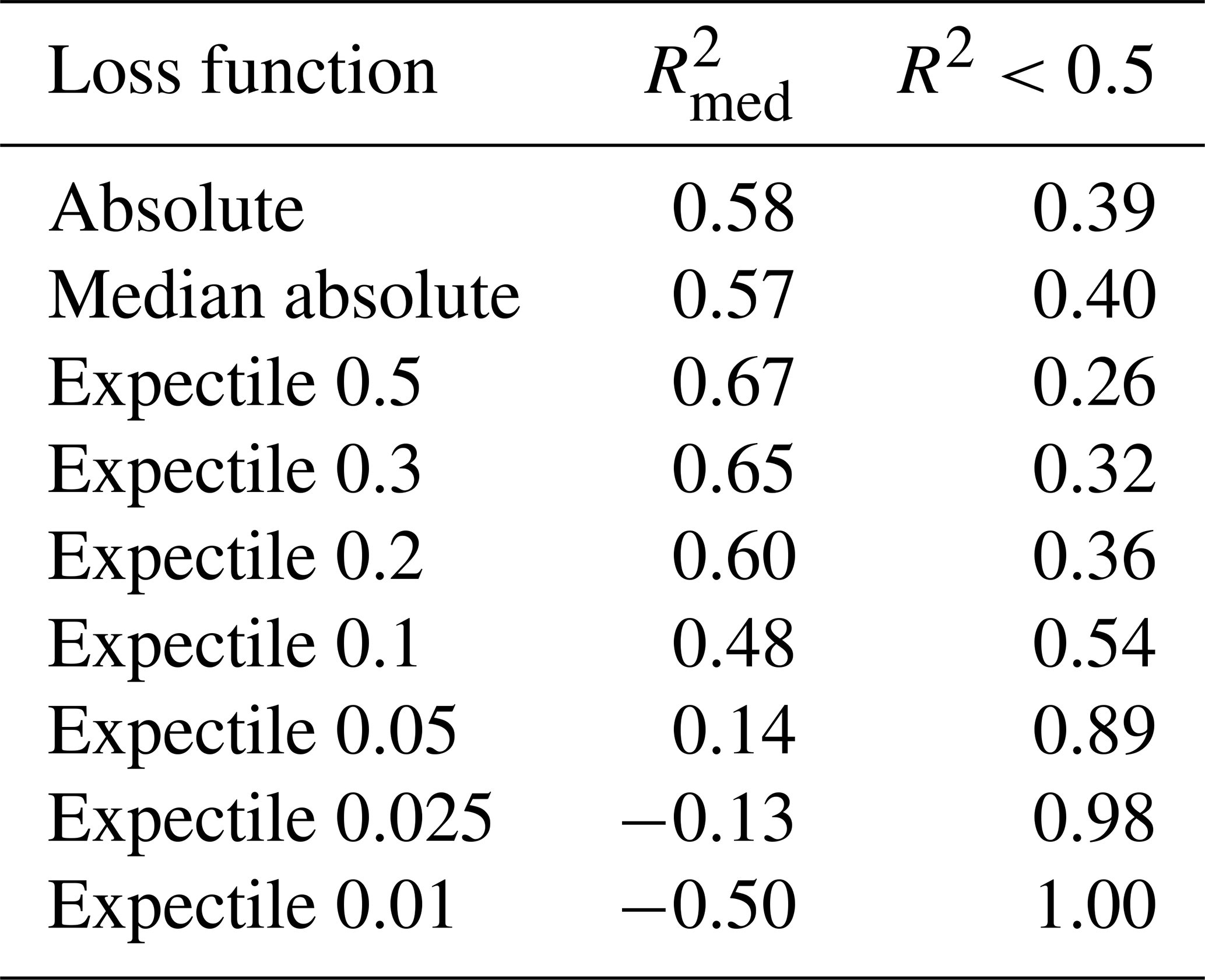
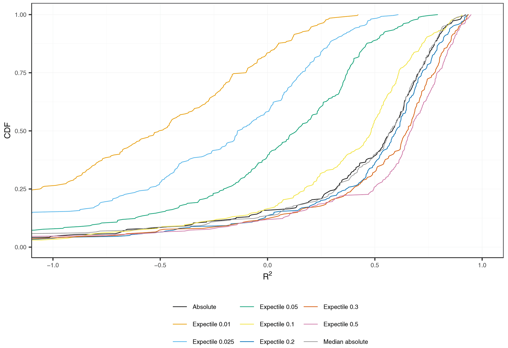
Figure 5 Empirical cumulative distribution function of station-wise R² by loss function across all stations. For improving visual clarity, the x axis is bounded at −1.

3.2.1 Error decomposition

For a better understanding of the error at the individual stations, we decompose the model error at each station into monthly, seasonal, annual fractions and a component representing the average error (prediction bias). Figure 6a gives an overview of the error components. For all expectiles, ${\mathit{\omega }}_{\mathrm{bias}}^{\mathrm{2}}$ and ${\mathit{\omega }}_{\mathrm{E}}^{\mathrm{2}}$ are the most important components. For the expectiles from 0.1 to 0.5, the ${\mathit{\omega }}_{\mathrm{E}}^{\mathrm{2}}$ is the main error contribution with median values between 52 % (0.1 expectile) and 59 % (0.2 expectile). The median values of ${\mathit{\omega }}_{\mathrm{bias}}^{\mathrm{2}}$ increases with decreasing τ, from 15 % to 19 % for the 0.5 to 0.2 expectiles, and 28 % for the 0.1 expectile. This trend continues for the smaller expectiles where the fraction of the mean error rises up to 56 % for the 0.01 expectile. At the same time, ${\mathit{\omega }}_{\mathrm{E}}^{\mathrm{2}}$ decreases for smaller expectiles, showing that expectiles with small τ are better fitted to the monthly values but predictions are generally less accurate. With median values around 10 % and between 3 % and 6 %, respectively, the seasonal and annual errors are much smaller than the mean error component and show a good performance of the models in predicting annual and seasonal low-flow variability.

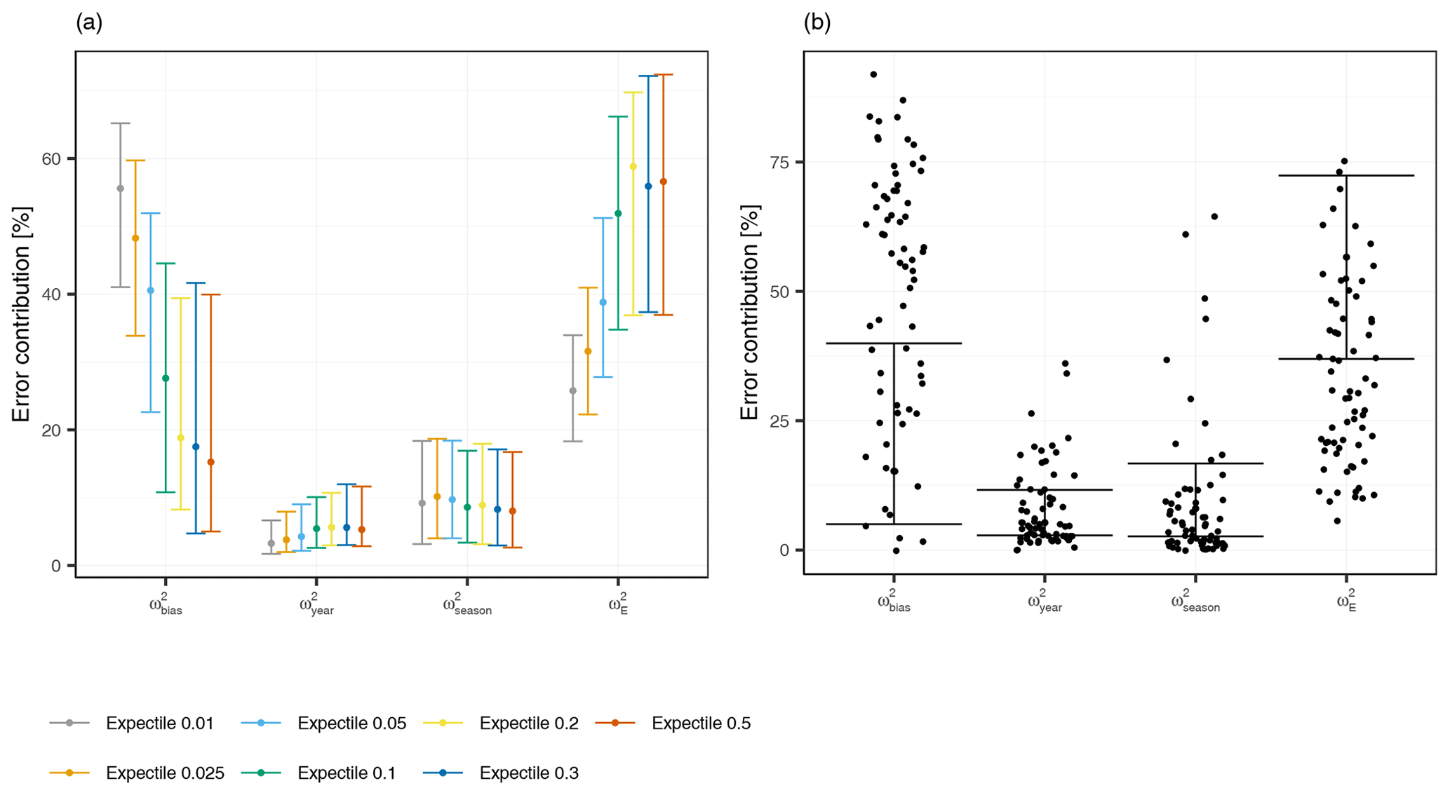
Figure 6 Error components of various expectile models. Panel (a) shows the relative error contributions for the season, year, month, and the bias part across all stations. The median (point) together with the 25 % quantile and the 75 % quantile (whiskers) of relative errors for each expectile loss function are shown. Panel (b) displays the error components for the 0.5 expectile in greater detail. The points are the stations which have a R² lower than 0.5.

An additional perspective comes from analyzing the share of stations showing only moderate or weak performance, as indicated by an R² of less than 0.5. As an example, Fig. 6b shows such ill-performing stations for the case of the 0.5 expectile model, with 67 stations (or 26 %) having an R² below 0.5. The main error contribution for these stations is the ${\mathit{\omega }}_{\mathrm{bias}}^{\mathrm{2}}$ with a median value of 56 %, which is much higher than the ${\mathit{\omega }}_{\mathrm{bias}}^{\mathrm{2}}$ of the well-performing stations (median value of 11 %). This again re-emphasizes the earlier finding that the main shortcoming of our modeling approach is an error in the mean, which reduces the predictive accuracy of the models. Seasonal and monthly variability, though, are well covered by the models, which is a strength of our spatiotemporal modeling approach.

3.3 Prediction of extremes

One objective of this study was the application of different expectiles for improving predictions at low extremes. This section will consequently focus on their evaluation. In a first step, we will filter our observations by only considering the observations at each station below a specific quantile. The filtered observations are then used to calculate an overall R², which is shown in Fig. 7. We can identify a huge performance advantage for low expectiles for predicting low extremes. For example, if we assess the accuracy of our models for cases below the 1 % quantile, the 0.01 expectile is yielding at least a R² of 0.42, where larger expectiles (0.05–0.5) show inefficient models with R² values below 0.1. What becomes apparent is that the performance is dropping at some point for the low expectiles (0.01, 0.025, 0.05), but is monotonically increasing for all other expectiles. Considering the results at the 25 % quantile, the R² of the 0.01 expectile decreased to 0.28, so that the best performance is at the 0.1 (0.53) and 0.05 expectiles (0.51). Further, we found that the 0.5 expectile has a lower performance than the 0.1, 0.2, and 0.3 expectiles, even for estimating the lower 50 % of the data.

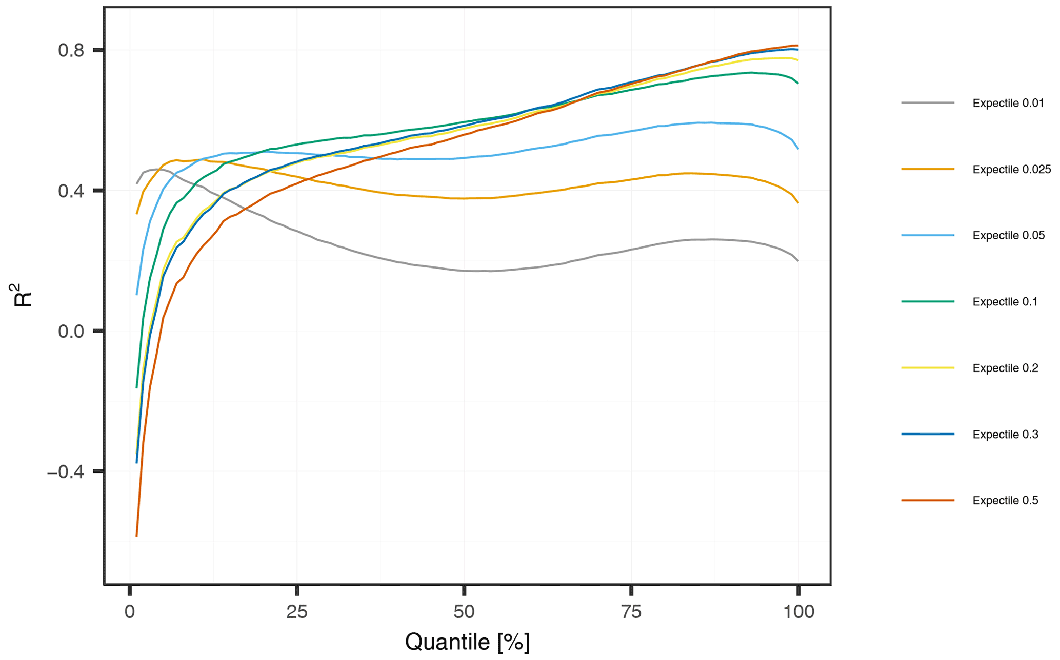
Figure 7 Global R² conditional to observations below low-flow thresholds. The thresholds are (station-wise) quantiles of the monthly time series with 1 % to 100 % non-exceedance probability.

Figure 8 EL_τ for τ=0.025, 0.05, 0.1 presented for all expectiles. The median, 25 % quantile, and 75 % quantile over all stations and each expectile are displayed.

As a second assessment of the predictive performance for low extremes, we compute the relative expectile error (EL_τ), a weighted error metric that distributes weights by expectile functions that have the greatest weight around τ. We choose τ values of 0.1, 0.05, and 0.025, as these approximately correspond to the q95_d, q98_d, and q99_d thresholds used for drought identification. Figure 8 shows the expectile errors EL_τ calculated for every station. Generally, the 0.1 expectile demonstrates a good performance by all EL_τ metrics. Smaller expectiles (0.01, 0.025, 0.05) perform as good or better than the 0.1 expectile for the EL_τ=0.025 (which gives most weight to most extreme events), but not for the other EL_τ metrics. Interestingly, the expectiles used for optimizing our loss functions do not perform best considering the respective EL_τ metric. For example, we would assume that the best-performing expectile for the EL_τ=0.025 would be the 0.025 expectile, but on median, this expectile yields a EL_τ=0.025 of 0.39, which is somewhat lower than the 0.1 expectile (0.4) or the 0.025 expectile (0.44). Furthermore, the smallest expectile (0.01) only obtains a median EL_τ=0.025 of 0.29, which is only slightly higher than the 0.2 expectile (0.28). Higher expectiles (0.2, 0.3, 0.5) show an increasing performance with higher τ, but their performance varies more across all stations. This suggests that one should choose an expectile function that gives most weight to somewhat higher values than the drought threshold of interest, and τ values around 0.1 appear most accurate for q95_d and q98_d drought events.

Figure 9 The predictions for the 0.01 and 0.5 expectiles are shown for station Au/Bregenzerach. The y axis is on a log scale for better visualization of the low extremes. Error metrics for the 0.5 expectile: R²=0.95, H_S=0.51, P_rec=0.79; 0.01 expectile: $R^{\mathrm{2}}=-\mathrm{0.07}$, H_S=0.94, P_rec=0.25.

In a final assessment of the model performance, we analyze the skill of the models to classify extreme events. For this purpose, we focus on the hit score (H_S) and the precision (P_rec) at each station. Table 5 shows the median of these two metrics over all stations and for all expectiles. Both skill scores decrease from less extreme (q95_d) to more extreme (q99_d) low flows for all expectiles. Concerning the effect of expectiles on P_rec and H_S, we see an opposite behavior, with H_S increasing towards the lower expectiles, and P_rec decreasing. For the lowest expectile (0.01), the H_S reaches 0.98, 0.94, and 0.9 for the three low-flow thresholds, respectively, showing that almost every observed drought event is identified. On the other hand, the P_rec is 0.2 for the q95_d and only 0.07 on median for the q99_d, which means that only 7 % of the predicted extreme events per station were actually extreme events. This points to an underestimation of extreme low flows when using low expectiles for model fitting. In contrast, using the 0.5 expectile would lead to an increase in the precision rate, but to a very low hit score. Figure 9 shows the contrasting properties of a high and low expectile model on low-flow predictions. The low expectile shifts the predictions to match the most extreme events but underestimates the moderate events. Clearly, such low expectiles result in strongly biased models with little practical relevance. These findings suggest a trade-off between accurate prediction of extremes, overall prediction accuracy and correct classification of extreme events, where the user needs to find some optimum.

Table 5 The precision P_rec and hit rate H_S are computed per station and the median is shown in the table for q95_d, q98_d, and q99_d.

3.4 Variable selection

The implemented RFE algorithm leads to a substantial reduction of variables. On median, the different expectiles require between 20 and 30 variables, except the 0.5 expectile that has a median of 35 variables. A closer examination of the static predictors (an overview of the selection of the static variables is given in Appendix A) shows that geological variables are never selected for any expectiles, and also from the land-use variables only the fraction of forest is selected frequently. However, a larger number of meteorological variables were selected over all expectiles: aridity index (AI, AI_sum), annual climatic water balance (MCWB), annual precipitation (P), and days with zero precipitation in the summer months (P_0,sum). Despite their frequent appearance in models, the performance gain of using meteorological variables for predictions is low, with a typical variable importance of less than 2 % for all models. In contrast, topological variables emerge as the dominant predictors in the model. The three topological variables yielding the largest performance gain in the models are the mean and maximum catchment altitude ($H_{\mathrm{M}},H_{+}$) and the mean catchment slope S_M. The variable importance for H_M is on average between 3.8 % and 4.4 % for all expectiles. A slightly increasing trend towards larger expectiles can be observed for S_M, with a variable importance of 10 % for the 0.01 expectile and on average 11.6 % for the 0.5 expectile. An opposed effect can be observed for H₊, where the variable importance decreases from 7.2 % for the 0.01 expectile to 4.3 % for the 0.5 expectile. Other topological predictors whose inclusion only had a minor influence on model performance are catchment area, latitude, longitude, and altitude of the gauging station, stream network density, and the fractions of flat, moderate, and steep slopes in the catchment.

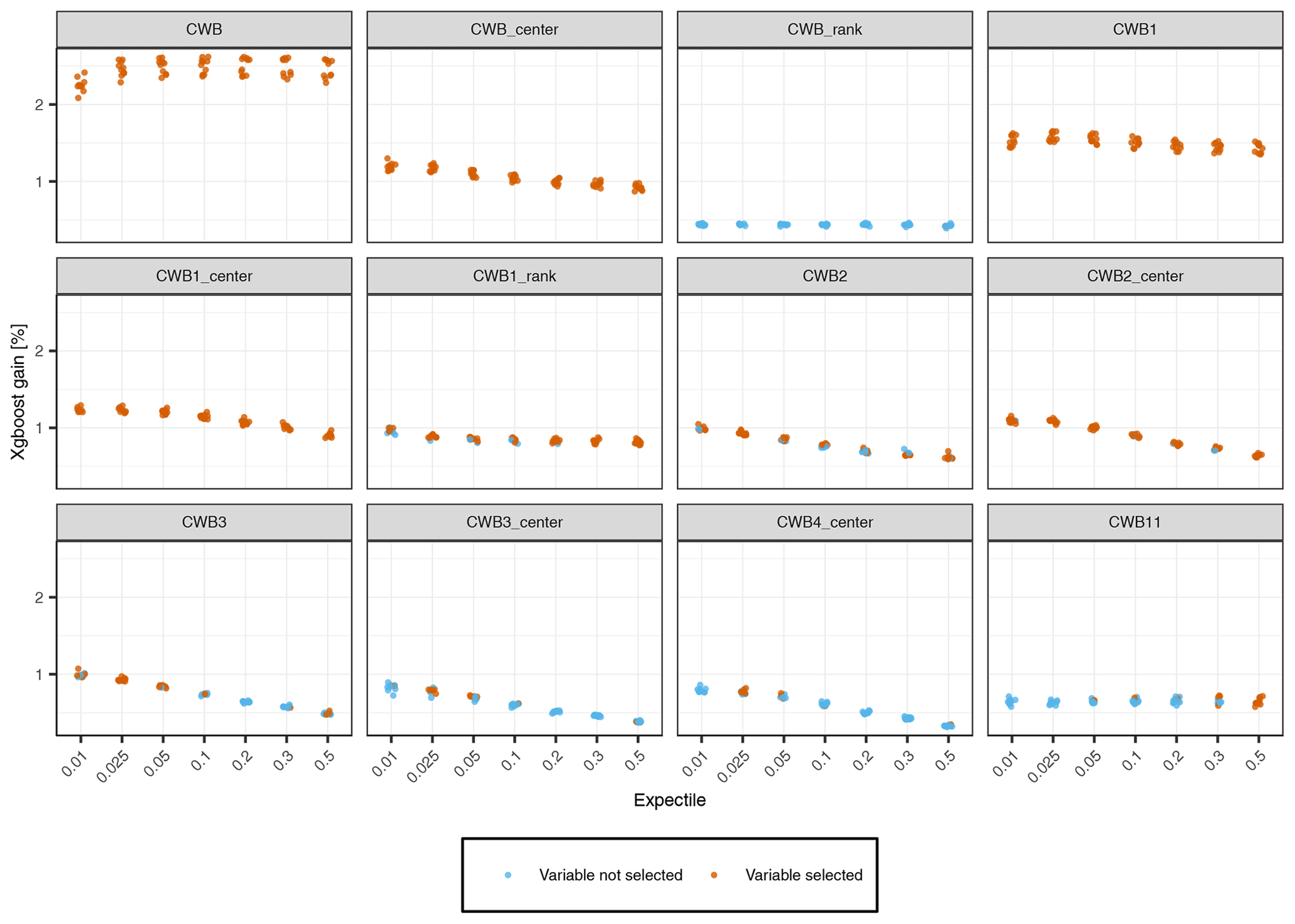
Figure 10 Selection of spatiotemporal variables that are used for different expectiles. For each expectile it is shown whether the variable is used for the final prediction of the fold or not.

Figure 10 shows an overview of the variable importance for the most relevant spatiotemporal predictors. The CWB is the most important variable with more than 2 % performance gain over all expectiles. The CWB_center, CWB₁, and CWB_1,center are also included in all models, but their variable importance is only 1 % to 1.5 %. Higher lags of the CWB are mainly included by the lower expectiles, but their performance gain is somewhat smaller and decreases with the lag of the variable. Comparing raw and standardized climate variables, the transformation of the absolute values to centered values seem to be beneficial in the case of the CWB, but this is not the case for the standardized drought indices, which were rarely selected and exhibited a low importance score in all cases.

4 Discussion

4.1 Value of expectile regression tree models for low-flow estimation

In this paper, we extended the extreme gradient boosting model XGBoost with the expectile loss function to develop a spatiotemporal model for low-flow predictions. We applied different τ values from 0.01 to 0.5 and evaluated their predictive quality in terms of overall performance, accuracy at extremes, and potential to classify extreme events in a time series. Our findings showed two contrasting behaviors. Larger expectiles such as 0.2, 0.3, and 0.5 showed better performance in respect to R² and $R_{\mathrm{med}}^{\mathrm{2}}$, whereas low expectiles (τ=0.01, 0.025, 0.05) led to a sharp decline in $R_{\mathrm{med}}^{\mathrm{2}}$ but increasing prediction accuracy at extreme low flows. However, optimization of the model cannot be reduced to these two criteria, as was shown in the further assessments. Low expectiles lead to a reduced precision at extreme low-flow events as a result of too many events being predicted. This suggests an overfitting of the lower tail of the low-flow distribution by low expectiles that reduces the predictive performance at the entire distribution. In contrast, the hit score drops sharply for higher expectiles, resulting in a low detection rate of extreme events. Therefore, the application of the expectile loss has to be considered carefully and adjusted to the specific research question. Figure 11 gives a synopsis of key performance metrics with respect to predicting q95_d, q98_d, and q99_d low-flow events. The synoptic representation nicely shows the trade-off between different performance metrics and puts the conclusions from their individual assessment into context. Depending on the low-flow event, a different optimum can be observed. When the focus of the study is on annual low flows in the order of q95_d, we see that the 0.2 expectile yields the optimal model fit, indicated by the crossing performance lines of the various metrics. However, when the purpose of the study is on predicting more extreme events (q98_d and q99_d), the 0.1 expectile is the optimal choice. These optima take into account the overall predictive performance ($R_{\mathrm{med}}^{\mathrm{2}}$) and emphasize the performance at the considered extreme, by the expectile loss, the hit rate, and precision at the event of interest. The optimized model shows a good performance in all metrics and appears well suited for spatiotemporal predictions of low-flow events.

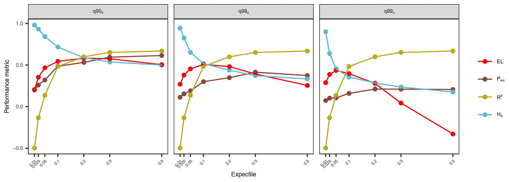
Figure 11 Overview of the error metrics EL_τ, P_rec, H_S, and $R_{\mathrm{med}}^{\mathrm{2}}$, plotted against every expectile. In each panel, H_S and P_rec are computed for the thresholds q95_d, q98_d, and q99_d. The EL_τ is calculated for the τ values of 0.025 (q95_d), 0.05 (q98_d), and 0.1 (q99_d).

4.2 Performance compared to literature

Performance evaluation in light of the existing literature is not straightforward, as we are not aware of any studies evaluating monthly low-flow models. Nevertheless, some studies did model the mean monthly streamflow, which we will use for comparison. Comparisons will be made on the NSE reported in these studies, which is an analogue measure to the R² in our study (Blöschl et al., 2013; Parajka et al., 2013). To put our monthly q95 models into context, we run an XGBoost model on monthly mean flow using the mean expectile regression (0.5) for our dataset. This leads to a median performance $R_{\mathrm{med}}^{\mathrm{2}}$ of 0.77 with only 15 % of the stations having an R² below 0.5. As expected, modeling monthly low flow shows weaker performance than modeling the mean monthly streamflow. Nevertheless, our results for q95 are still in the range of published studies on mean monthly streamflow models. For example, Cutore et al. (2007) found NSE values ranging from 0.57 to 0.78 by modeling 9 basins in Italy using ANNs. A similar performance has been reported by Pumo et al. (2016) for 59 stations in Sicily, Italy. They modeled monthly streamflow by interpolating regression parameters to ungauged basins and their NSE values ranged from 0.7 to 0.8 for 6 selected validation stations. A comparative assessment of regionalization approaches for hydrological models at 22 stations in the USA (Steinschneider et al., 2015) showed NSE values ranging from 0.6 to 0.85. Note that these results were obtained for relatively small datasets under quite homogeneous hydrological conditions. In our study, low-flow predictions were evaluated on a larger, diverse hydrological dataset and we found similar performance metrics to those in the aforementioned studies.

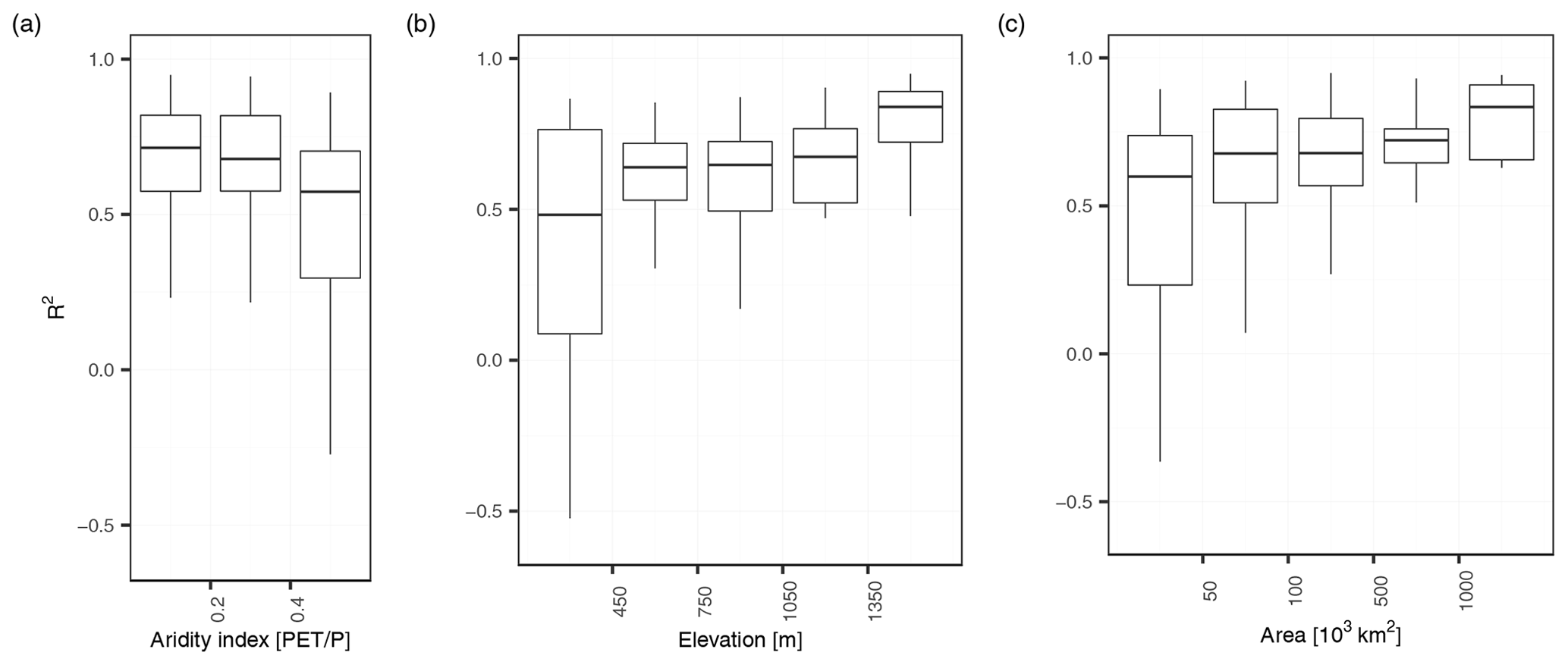
Figure 12 Panels (a), (b), and (c) show R² per station of the 0.5 expectile plotted against the aridity index, elevation and the area. In all plots, outliers are not included for a better visualization.

A more qualitative embedding to the scientific literature can be made by integrating our findings into the comparative evaluation of regionalization procedures of Parajka et al. (2013). Parajka et al. (2013) evaluated the performance of runoff-hydrograph studies, mostly performed on a daily time step, as a function of aridity, elevation, and catchment area to assess the extent to which performance depends on main climate and catchment characteristics. Figure 12 shows our finding in context of these three catchment characteristics. Parajka et al. (2013) found a decreasing performance with higher aridity. In our study, the aridity index is below 0.6 for all our catchments, but shows a similar decrease in performance. In our study, the performance increases with catchment elevation, with catchments below 450 m a.s.l. having the lowest performance ($R_{\mathrm{med}}^{\mathrm{2}}$ of 0.5) and catchments above 1350 m a.s.l. the highest performance ($R_{\mathrm{med}}^{\mathrm{2}}$ of 0.8). The increase in performance with elevation points to a higher performance for catchments with dominant winter low-flow seasonality, which can be explained by their more regular and thus better predictable regime. We can indeed observe a lower performance for stations with a summer low-flow regime ($R_{\mathrm{med}}^{\mathrm{2}}=\mathrm{0.63}$) than for stations with a winter low-flow regime ($R_{\mathrm{med}}^{\mathrm{2}}=\mathrm{0.73}$). However, in a stratified assessment of summer and winter months, we could not find any difference in performance, neither in the entire study area, nor for summer- and winter-dominated catchments separately. This is in contrast to Staudinger et al. (2011), who found a reduction in model performance for summer months compared to winter months for a Norwegian study area with conditions comparable to the mountainous catchments in our study. Finally, we also found more accurate model predictions for larger basins. These are not due to a simple size effect of catchment area on discharges, since we use specific low flows as target variable to make catchments of different size more comparable. Many of our small catchments are located in a karstic environment or moors, which exhibit highly irregular regimes that are particularly hard to regionalize. Larger catchments, in contrast, have a more regular regime and show a high prediction performance.

5 Conclusions

In this paper, we analyzed the performance of a single spatiotemporal XGBoost model on the prediction of monthly low flow for a comprehensive dataset of 260 gauging stations in Austria. We paid particular attention to the estimation of low extremes, by applying the expectile loss function as a fitting criterion. Our results show that the expectile loss yields a high prediction accuracy, but the performance decreases strongly for small expectiles. The best-performing model is the 0.5 expectile with a $R_{\mathrm{med}}^{\mathrm{2}}$ of 0.67, but also the 0.2 and 0.3 expectile reach a higher $R_{\mathrm{med}}^{\mathrm{2}}$ than the mean and median absolute loss. Small expectiles such as 0.01 or 0.025 already yield a negative $R_{\mathrm{med}}^{\mathrm{2}}$, resulting in a high number of poor-performing stations.

Weak-performing stations can also be found for the 0.5 expectile, where 26 % of the stations have an R² below 0.5. A decomposition of the model error revealed that the monthly error is the main error component for large expectiles, while the seasonal and annual components are negligible for most stations. Considering the weak-performing stations of the 0.5 expectile, the dominant error component is a systematic error or bias. With a median value of 56 %, the bias is much larger at these stations compared to well-performing stations with a median value of only 11 %. This underlines the finding that the main shortcoming of our approach is a systematic error, which impairs the predictive accuracy. However, the strength of our spatiotemporal model is the good approximation of the seasonal and annual variability of monthly low flows, as shown by the low seasonal and annual error component.

Despite the low global performance of small expectiles (τ=0.05, 0.025, 0.01), they demonstrate an increasing accuracy when focusing on low extremes. This improvement in predictive performance has the simultaneous disadvantage that extreme low flows are increasingly misclassified. We found that the application of the expectile loss results in a trade-off between global performance, prediction accuracy of extremes, and misclassification rate of extreme events. The implementation of the 0.1 or 0.2 expectiles, depending on whether we want to optimize predictions for annual or more extreme low flow, appears to be optimal with respect to all criteria. The resulting extreme gradient tree boosting model covers seasonal and annual variability nicely and provides a viable approach for spatiotemporal modeling of a range of hydrological variables that represent average conditions and extreme events.

We demonstrate that the expectile loss is a suitable alternative to common loss functions in spatiotemporal low-flow models. However, its application is not limited to statistical learning models such as XGBoost, but can also be considered for hydrological models when their focus is on predicting hydrological extremes. As with all models, there is a trade-off between overall predictive performance, accuracy on the tails of the distribution, and identification of extreme events that should be considered in model applications.

Appendix A

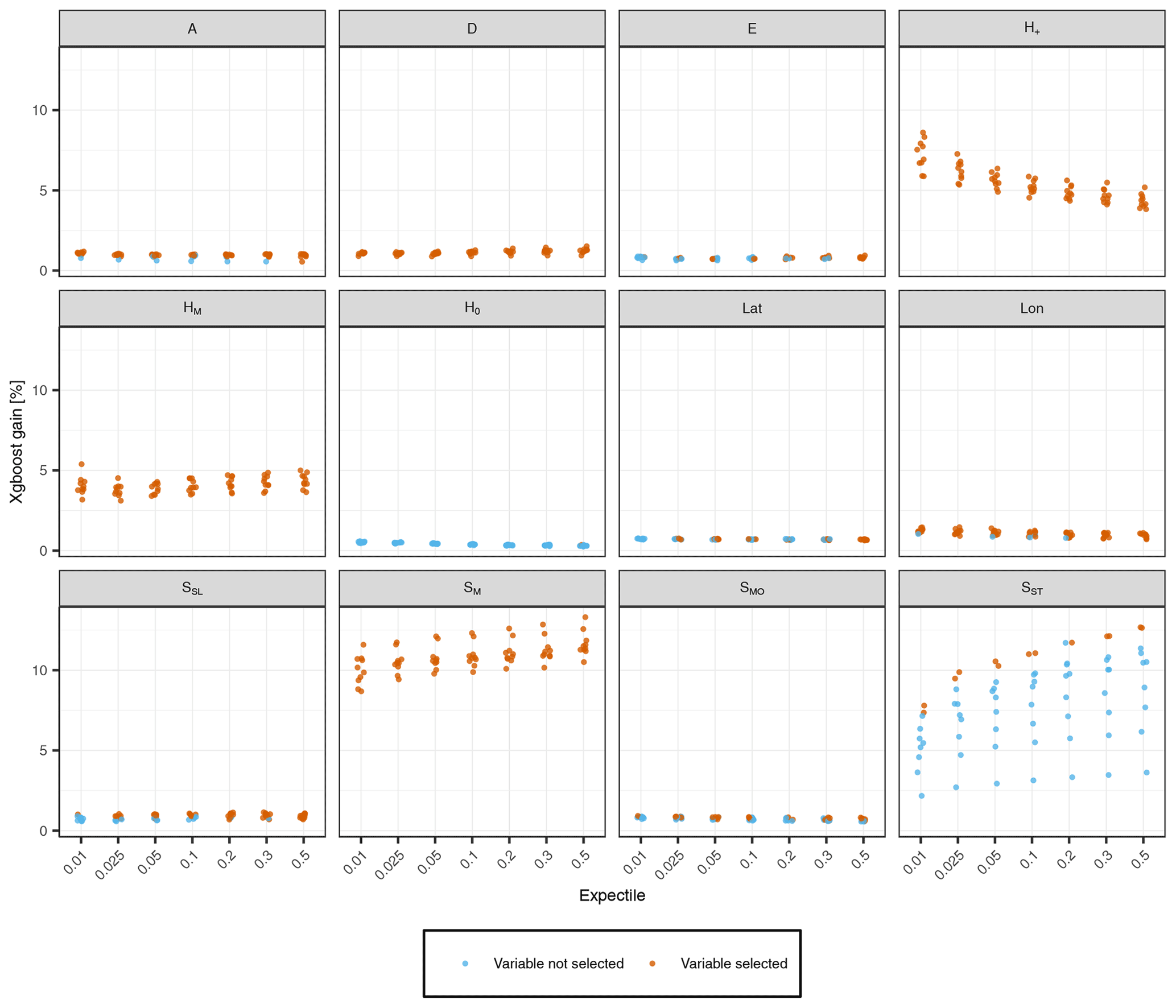
Figure A1 Predictive power of static topological predictors obtained by the backward variable selection procedure (Sect. 2.2.3). The performance gains of the 10 prediction folds per expectile model are shown, with colors indicating whether the variable is used for the final prediction of the fold or not. Variables that were never selected by our model are not shown.

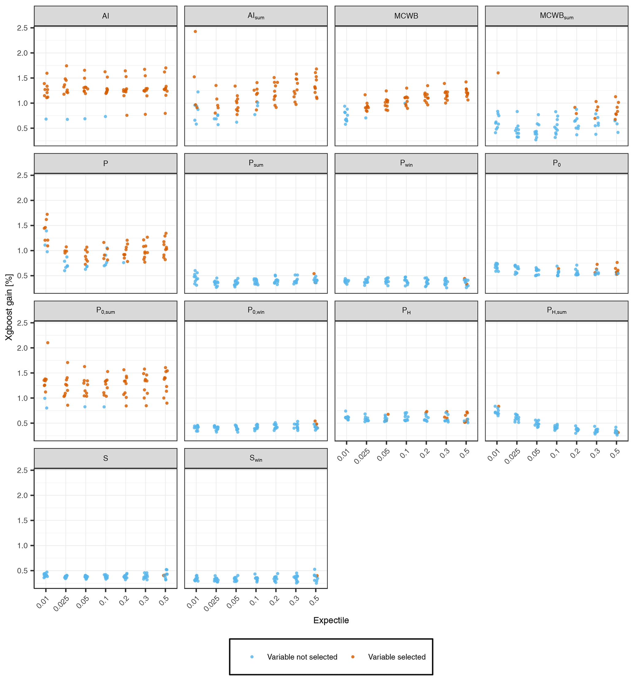
Figure A2 Predictive power of static meteorological predictors obtained by the backward variable selection procedure (Sect. 2.2.3). The performance gains of the 10 prediction folds per expectile model are shown, with colors indicating whether the variable is used for the final prediction of the fold or not. Variables that were never selected by our model are not shown.

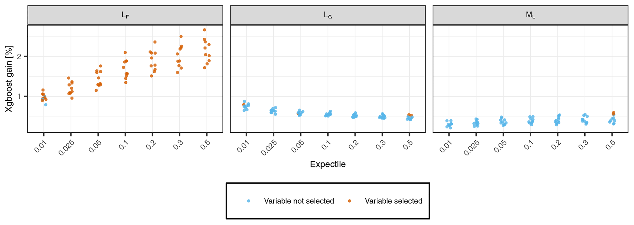
Figure A3 Predictive power of static land-use predictors obtained by the backward variable selection procedure (Sect. 2.2.3). The performance gains of the 10 prediction folds per expectile model are shown, with colors indicating whether the variable is used for the final prediction of the fold or not. Variables that were never selected by our model are not shown.