the Creative Commons Attribution 4.0 License.
the Creative Commons Attribution 4.0 License.
 | 31 Jan 2022
Rediscovering Robert E. Horton's lake evaporation formulae: new directions for evaporation physics
Solomon Vimal
Vijay P. Singh
Evaporation from open water is among the most rigorously studied problems in hydrology. Robert E. Horton, unbeknownst to most investigators on the subject, studied it in great detail by conducting experiments and heuristically relating his observations to physical laws. His work furthered known theories of lake evaporation, but it appears that it was dismissed as simply empirical. This is unfortunate because Horton's century-old insights on the topic, which we summarize here, seem relevant for contemporary climate-change-era problems. In rediscovering his overlooked lake evaporation works, in this paper we (1) examine several of his publications in the period 1915–1944 and identify his theory sources for evaporation physics among scientists of the late 1800s, (2) illustrate his lake evaporation formulae, which require several equations, tables, thresholds, and conditions based on physical factors and assumptions, and (3) assess his evaporation results over the continental U.S. and analyze the performance of his formula in a subarctic Canadian catchment by comparing it with five other calibrated (aerodynamic and mass transfer) evaporation formulae of varying complexity. We find that Horton's method, due to its unique variable vapor pressure deficit (VVPD) term, outperforms all other methods by ∼3 %–15 % of R2 consistently across timescales (days to months) and at an order of magnitude higher at subdaily scales (we assessed up to 30 min). Surprisingly, when his method uses input vapor pressure disaggregated from reanalysis data, it still outperforms other methods which use local measurements. This indicates that the vapor pressure deficit (VPD) term currently used in all other evaporation methods is not as good an independent control for lake evaporation as Horton's VVPD. Therefore, Horton's evaporation formula is held to be a major improvement in lake evaporation theory which, in part, may (A) supplant or improve existing evaporation formulae, including the aerodynamic part of the combination (Penman) method, (B) point to new directions in lake evaporation physics, as it leads to a “constant” and a nondimensional ratio (the former is due to Horton, John Dalton (1802), and Gustav Schübler (1831) and the latter to Jožef Štefan (1881) and Horton), and (C) offer better insights behind the physics of the evaporation paradox (i.e., globally, decreasing trends in pan evaporation are unanimously observed, while the opposite is expected due to global warming). Curiously, Horton's rare observations of convective vapor plumes from lakes may also help to explain the mythical origins of the Greek deity Venus and the dancing Nereids.
- Article
(2215 KB) - Full-text XML
-
Supplement
(256 KB) - BibTeX
- EndNote


The problem of accurate lake or open water evaporation estimation has been a subject of scientific inquiry, in the modern sense of combined experimental and theoretical study, for the past 4 centuries. Factors that control evaporation have been investigated since the time of Edmund Halley (1687), with rapid progress in theories of thermodynamics, aerodynamics (turbulence theory), and molecular kinetics (kinetic theory of gases) that led to a better understanding of evaporation due to wind's influence, convection, and diffusion. Brutsaert's (1982, chap. 2) treatise on Evaporation Into the Atmosphere provides an overview of the concepts that have evolved from antiquity. Since the 1700s, key contributions have included those of Johann and Daniel Bernoulli (1700s), John Dalton, Rudolf Clausius, and Osborne Reynolds (1800s), who began the celebrated voyage through turbulence theory (Davidson et al., 2011) from European, American, and Russian schools, among others, especially as the data of field experiments on surface winds and diffusion became increasingly crucial for chemical warfare efforts over the course of the 20th century (Sutton, 1953). More recent developments include the recognition of the complementary principle of evaporation in the late 1900s (Bouchet, 1963; Morton, 1994; Brutsaert, 1982) and the evaporation paradox (Roderick and Farquhar, 2002), which have large implications in climate change debates.
Robert E. Horton, a pioneer in hydrology and well regarded for his contributions to areas of hydrology like infiltration, overland flow, and river geomorphology, is not usually considered a fundamental contributor to the field of evaporation. However, unbeknownst to most in mainstream evaporation theory, tucked away in his home-based experimental catchment beside a pond, Horton conducted rigorous experiments and theoretical work on open water evaporation from the 1910s until the end of his career (circa 1945). In particular, in 1917, he published a set of formulae for estimating evaporation (including within-lake variations in evaporation) based on physical laws which he believed were more robust than the then existing methods. The subheading to the title of his first 1917 paper claims the following:
Empirical Statement Based on Physical Law Agrees with Observed Facts and Is Held To Be an Improvement Over Existing Formulas (Horton, 1917a).
He held the view that his equation was superior to other known methods for the following decades, even in the face of rapid developments in evaporation theory in that period (e.g., see Horton, 1934). After we examined several of Horton's papers and reports related to evaporation from lakes and pan evaporimeters (or, simply, pans) from 1917 to 1944 (the year before his death), we noted that he derived his formula theoretically, but since the values of the coefficient in his formula were not easily available, and his formula resembles other empirically derived formulae, several investigators may have dubbed it as simply empirical (see Rohwer, 1931). However, Horton's nuanced understanding of the boundary layer physics of his time (turbulence theory, horizontal vapor transport via laminar flow, convective transfer of vapor, and wind and vapor blanket characteristics), and the sound premise of his work based on molecular kinetics, reveal the potential of his work to offer new insights for an improved formulation of evaporation. The theory behind his work is illustrated in Sect. 2. After evaluating Horton's evaporation formulae (in Sect. 3), we find that his claim of having developed an improved method not only stands to be true in his time but also holds great contemporary value, and it is unfortunate that it has been largely overlooked or forgotten. Therefore, in this paper, we examine his evaporation work from the perspective of contemporary theories and those of his time to highlight his ingenious perceptual, experimental, and theoretical insights into the subject. We revisit his claims, replot his figures with recent data, simplify the use of his experimental tables (by converting them to parametric forms), assess his method's ability to generalize across wide-ranging conditions, and show the relevance of his method for contemporary large-scale evaporation problems.
1.1 Horton's broader contributions and bibliography
Hydrologists need no introduction to some of Horton's contributions like infiltration theory, overland flow, and geomorphological laws, but what may not be widely known is that he published an estimated 200 papers and reports, and of these, only about 80 works (mostly single authored; ∼90 %) are available from readily accessible sources (Hall, 1987). Horton's unpublished works are held at the U.S. National Archives in College Park, Maryland (cataloguing and organization was done by Walter Langbein). A subset of his archive is also held at his alma mater, Albion College (Accavitti, 2019). In the last few decades, Keith Beven from Lancaster University and Jim Smith from Princeton University examined a portion of the archive contents and presented their findings via publications (Beven, 2004a, b, c) and an American Meteorological Society (AMS) Horton Lecture (Smith, 2011).
About 80 of Horton's contributions were provided by Hall (1987) and curated by the American Geophysical Union (AGU) Virtual Hydrologist Project (see Foufoula-Georgiou (Foufoula-Georgiou, 2021; Folse, 1929). A more complete list of Horton's works was collated by Elizabeth Clark, which includes ∼135 works, for an AMS Horton Lecture delivered by Dennis Lettenmaier (2008). Combining these lists and conducting additional searches, the first author collated 168 works, which is the most comprehensive list of Horton's works available to our knowledge. Years and titles are shared in the Supplement, together with some tips on how to conduct an effective search to find Horton's papers and their full citations.
1.2 Horton's lake evaporation method and related projects
About a dozen of Horton's papers and reports are related to his evaporation method and supporting ideas, but one can gain a full understanding of his published contributions on lake evaporation from five key publications (i.e., Horton, 1917a, 1927, 1934, 1941b and 1943b). Horton's evaporation method was first introduced in Horton (1917a), as part of a three-paper series (Horton, 1917a, b, c) in Engineering News-Record, for the purpose of improving waterpower, water supply, and irrigation projects. The larger goal of the three papers was to reduce errors in estimates of stream yield, especially to gain accurate estimates of low flows to ensure the success of hydraulic (water supply) projects. This goal necessitated reliable evaporation estimates, leading Horton to develop his own method to calculate it. The tables needed to implement his method were not published in their entirety in Horton (1917a) but only in a later report on the Great Lakes a decade later (Horton, 1927), which was a major project in his career that involved a rigorous procedure for lake evaporation estimation among a broader hydrological study of the Great Lakes. This work was conducted in collaboration with Carl E. Grunsky and was an extensive 432-page report. The central innovation of this contribution is that, prior to this work, it was not possible to achieve correlations between discharge and lake levels which are impacted by a variety of natural and artificial causes. A substantial portion of the report is a presentation of available data related to the hydrology of the Great Lakes and the remainder is an analysis of various aspects of the water balance (precipitation, runoff, and evaporation), including 142 tables and 73 figures. In another paper 7 years later, Horton (1934) provided more theoretical insights into his evaporation method with an explanation of its physical basis. Besides these major works on the evaporation method, projects where he examined lake evaporation spanned earlier and later times in his career. For example, in Horton (1905), he discusses evaporation in the context of draining of kettle ponds (small ponds formed as a result of deglaciation), and in Horton (1944), he estimated evaporation for dam design for the Hemlock Lake water supply system in Rochester, New York. As a final point to contextualize his lake projects, Horton's experimental catchment beside his house included a pond about 200 m long and 60 m wide (a figure is provided in Horton, 1919a), where he conducted evaporation experiments and interesting observations. We revisit this in our paper's closing note (Sect. 7).
1.3 Previous examinations of Horton's lake evaporation method
The various above-mentioned works related to lake evaporation have been cited sparingly which shows that they were largely overlooked. They have not been collectively examined in any previous work to our knowledge, and in the few citations to them, the value and sophistication of the method was not recognized. Horton's lake evaporation equation received some attention in Chow's (1964) Handbook of Applied Hydrology (in Sect. 11 on evaporation written by Frank J. Veihmeyer). Horton's formula is surprisingly not included in Brutsaert's (1982) treatise, which has ∼650 citations of evaporation-related works, though his work on evaporation pans has been cited, referencing standardized class A pans. The equation was cursorily reviewed in a few recent studies. McMahon et al. (2016) cite the equation (presumably taken from Rohwer, 1931), as part of a larger review, together with other evaporation equations. Singh and Xu (1997) evaluated Horton's evaporation equation in comparison with 12 other (mostly) empirical equations that resemble it, but incorrectly, in the sense that the vapor pressure deficit (VPD) was multiplied with the wind factor, whereas, for the correct use of Horton's equation, the wind factor is to be multiplied with the vapor pressure of water and not the total deficit; this is a fundamental difference between his method and other methods (as will be explained in Sects. 2 and 3 in more detail). As inferred from citations to his key evaporation paper (Horton, 1917a) via Google Scholar (https://scholar.google.com/, last access: 29 April 2021), a few investigators from Russia and Portugal have examined his evaporation work, and one particular work from Japan (Siomi and Yosida, 1940) seems to have examined Horton's equation in some detail but not as comprehensively as we undertake here. All these works do not account for the full complexity of his approach; for a comprehensive use of Horton's lake evaporation method, about 20 equations and two tables are needed (Sects. 2 and 3). One of these tables was not very accessible, as it was published in a report (Horton, 1927) which, presumably, was not as widely circulated as an academic journal, which may have led to the limited use of his method.
1.4 Mainstream evaporation works in Horton's time
For a context of the works preceding Horton's time, interested readers are directed to an excellent contribution by Grace Livingston, published as eight pieces in Monthly Weather Review between 1908 and 1909 and later compiled into a book (see Livingston and the United States Weather Bureau, 1910). This annotated bibliography includes ∼850 works on evaporation from the late 1600s up to the early 1900s, lists 155 publication outlets, and was translated from multiple world languages (Japanese, French, Italian, German, and Russian, among others). It is possible that Horton considered his equation as being an improvement over other evaporation formulae presented in this review. Horton did not cite this bibliography in any of his evaporation papers, but there are multiple reasons to speculate why he might have examined it. (1) Many of Horton's works were published in the same journal (Monthly Weather Review). (2) He followed an unconventional citation style and often included no reference lists in his papers (e.g., see Horton, 1917a). (3) Grace Livingston was the ex-wife of a plant physiologist, Burton E. Livingston, whose work on evaporation Horton certainly followed (Horton, 1927). (4) The compiled book format of the annotated bibliography was available at the U.S. Weather Bureau (Washington, D.C.), which published the compilation (Livingston, 1910), and the John Crear Library in Chicago, which are places that Horton presumably frequented due to their proximity to the work he did in Chicago and his engagements with members and initiatives of the Weather Bureau (Horton, 1927). Finally, (5) most, if not all, of the theoretical sources that Horton's evaporation method relied on (discussed later in see Sect. 1.5) appear in one place, that is, in Livingston's and the United States Weather Bureau (1910) work.
Horton's evaporation method was apparently developed and used in New York, Michigan, and Chicago (see Horton, 1927), but, in the same time period, many similar efforts were underway throughout the United States (presumably in other countries too). Worth highlighting are the following three works: First, there is the thermodynamic approach, using Le Châtelier's principle applied to energetics. This approach, which was undertaken in California at the Scripps Institute of Oceanography and California Institute of Technology, led to the energy balance solution of lake evaporation and the Bowen (1926) ratio. Subsequent works by others that picked up on this work are summarized in a succinct compendium by McEwen (1930) and a historical summary by Lewis (1995). Second, there is a review of mass-transfer-based and energy-balance-based evaporation studies on Lake Hefner, resulting from collaboration between several U.S. agencies, including the Geological Survey, Department of Navy, Bureau of Ships, Navy Electronics Laboratory, Department of Interior, Bureau of Reclamation, Department of Commerce, and Weather Bureau (USGS, 1954). Third, there is a statistical attack on the problem led by geophysicist John. F. Hayford, who notably spent over 2000 h developing a superior method, including a mammoth effort by 41 persons, who collectively spent some 32 000 h on this work (Folse, 1929, p. 7). The method uses the temperature and humidity of the preceding day to calculate the following day's evaporation, and includes a large system of equations with many free parameters, which is optimized to minimize error (for more details, see Folse, 1929). It was developed for the Great Lakes, and did perform reasonably well there, but generalized poorly in other lakes and did not gain wider attention (see the critical review by Bernard, 1936). These highlight some of the various independent efforts dedicated to calculating evaporation around the time when Horton's method was developed.
1.5 Horton's main sources for theories and experiments of lake evaporation physics
Citations provided in Horton's work show that he relied on the works of several European scientists for the concepts related to the physics of evaporation. He did examine several empirical equations developed in the U.S. (see Horton, 1934), but he does not appear to have followed the works conducted by Bowen and Cummings (Bowen, 1926). Perhaps this is because Bowen's works appeared in Physical Review, while Horton published his works in Monthly Weather Review. Moreover, Horton's approach differed in that it was premised on aero-hydrodynamics and kinetic theory approaches, which were developed mainly by European scientists.
A molecular kinetics view of evaporation is fundamental to Horton's approach, and he developed this view mainly from John Dalton's (1802) theories and experiments on evaporation of water and other chemicals. Dalton's (1802) work was, in fact, the only work that Horton directly cited when he first published his evaporation paper (Horton, 1917a), though, with a closer look at his later papers (Horton, 1927, 1933), it does appear that he developed his method by building upon multiple works. It appears that Horton studied the following works: he consulted Thomas Stevenson's (1882) work on wind speed variation by height, while conducting his own experiments on the role of wind on evaporation (see Horton, 1927); he referred to the work of Geoffrey Ingram Taylor and William Napier Shaw (1918), for the role of turbulence and the vapor blanket (Horton, 1934); he drew from Napier Shaw's work in Manual of Meteorology (Shaw and Austin, 1932) and Julius von Hann's work in Lehrbuch der Meteorologie (von Hann, 1926), for more on psychrometry (see Horton, 1934, and also Horton, 1921, though no citations are provided in the latter); he consulted Thomas Tate's (1862) work, for the laws of evaporation; and he derived value from the work of Jožef Štefan (1882), for his analysis on the water surface's geometric controls on evaporation and also, perhaps, the role of the vapor blanket in turbulent and convective transfer of vapor from large and small water bodies. Štefan is cited in Horton (1934), but Štefan's work may have also inspired the equations in Horton (1917a), due to their resemblance. A reference to a chemistry book he read in his youth (from his short story collection; see Horton, 1938) can be traced to A Dictionary of Chemistry and the Allied Branches of Other Sciences by Henry Watts (1882), wherefrom Horton learned about a sampling method to collect combustible marsh gases from shallow ponds and lakes. In a posthumous work on convectional vortex rings (van Vliet and Horton, 1949), he uses Peter G. Tait's acid experiment to understand convection (Tait lecture, 1878; referenced in Dolbear, 1892 and Risteen, 1896) which gives one a mental picture of how Horton viewed convective evaporation from lakes. From these references, we can see how Horton's physical chemistry knowledge developed over the course of his life.
Horton's references also included American textbooks, particularly the following two: Allen Risteen's (1896) Molecules and Molecular Theory of Matter and Amos Emerson Dolbear's (1892) Matter, Ether, and Motion. Risteen's (1896) work is cited in Horton (1934), where his evaporation formula is discussed in more detail than in previous papers. It appears that Horton's collaborator, Richard van Vliet, who published Horton's work on convectional vortex rings posthumously (van Vliet and Horton, 1949), misspelled his reference to Dolbear as Dalhaer (perhaps a transcription error). These American textbooks referred to theories developed in Europe by Rudolf Clausius and a treatise on the kinetic theory of gases (Watson, 1876). Watson's work on kinetic theory, in turn, credits the origin of these theories to Johann Bernoulli, James Clerk Maxwell, Rudolf Clausius, and Ludwig Boltzmann. Most of these scientists were aerodynamicists, physicists, and chemists. Notably, Dolbear was not only a physicist but also a pioneering inventor, who competed with Alexander Graham Bell at the Supreme Court of the U.S. for priority on the patent of the telephone (his claim was that he invented it 10 years earlier, but he lost the case). Nearly all of these books are available for free from Google Books (references and hyperlinks are provided in the reference list).
Before we delve into the details of the evaporation equation, the following quote from Horton contextualizes how he supposedly viewed his evaporation formula:
A rational equation may be defined as one which can be derived directly from fundamental principles, which fits all the experimental data and which represents the physical conditions correctly throughout the entire range of their occurrence and hence is valid outside the range of experimental observation. (Horton, 1941a)
Some fundamental principles that he alluded to in his evaporation formula are related to thermodynamics (i.e., work done in phase changes and latent heat), and they include references to geometric proofs of these principles from the perspective of kinetic theory drawn from Risteen (1896), as discussed in Horton (1934). More importantly, the premise of Horton's fundamental principles in his evaporation method is the kinetic theory of gases (Loeb, 1934), which he explicitly stated in Horton (1917a). His molecular kinetics view of evaporation is best captured by the following quote:
In a mixture of air and water-vapor there is a certain number of vapor molecules per unit volume. When there is wind the air and vapor are swept along together at a rate depending on the pressure-gradient. This, as in case of hydraulic flow, is independent of the total pressure. At a given vapor-pressure the same amount of vapor is carried by the wind per unit of time and per unit of volume of air, whether the number of air molecules per unit volume is large or small. (Horton, 1934)
Horton considered the movement of molecules and their behavior at the surface of the lake as three key processes, i.e., (1) vapor emission, (2) vapor removal (by diffusion, convection, and wind action), and (3) vapor return. These processes are discussed in multiple papers (Horton, 1917a, 1934). It may benefit the reader to review these three processes in some detail before we introduce the evaporation equations in Sect. 3.
2.1 Vapor emission and vapor return
His first paper on evaporation (Horton, 1917a) does not discuss the thermodynamic perspective, but his derivation of the various parts of the evaporation equation does use the underlying principles, as exemplified in the following quote:
[Latent heat] comprises of two elements: (1) Internal work in overcoming molecular attractive forces which, in general, including viscosity and surface-tension, increase as the temperature decreases, and the latent heat of internal work also increases as the temperature decreases; (2) the external latent heat, which measures the work done by the emitted vapor in expanding against the external pressure, decreases slightly as the pressure on the liquid surface decreases with decreased boiling temperature, but the total latent heat increases slowly as the temperature decreases. (Horton, 1934)
He examined these thermodynamic factors to identify the role of pressure in impacting vapor emission and vapor removal. While pressure does affect vapor emission rates due to external latent heat, it is negligible, so the impact of pressure on evaporation can be attributed to vapor removal (somewhat like a proof by elimination).
Vapor return is controlled by wind action (which is nonlinear) and the vapor pressure of the overlying air or the vapor blanket, i.e., a thin layer of vapor just above the water surface analogous to viscous sublayer in open channel flow. The characteristics and role of the vapor blanket is discussed separately and in more detail in Sect. 3.4.
2.2 Vapor removal
Vapor removal, as previously stated, happens due to diffusion, wind action, and convection.
2.2.1 Diffusion
Horton's conception of evaporation via diffusion is perhaps drawn from Dalton's (1802) original work, which is the only reference he cites when he first published his lake evaporation formula in Horton (1917a). Dalton posited the following:
Evaporation […] is caused by vis inertiae of the particles of air; and is similar to that which a stream of water meets with in descending amongst pebbles […]. From a great variety of experiments [on evaporation,] I have found the results entirely conformable with the above theory […] (Dalton, 1802, 581–584)
The rate of diffusion is governed by water temperature (for vapor emission rate) and barometric pressure and vapor pressure of air (vapor return rate), and is not explicitly affected by wind action or convection (Horton, 1934).
2.2.2 Wind action
According to the contemporary evaporation literature (see Brutsaert, 1982), wind can have two effects, namely (1) turbulence transfer of vapor away from the surface and (2) advective (bulk fluid mass) transport due to mean horizontal wind. In Horton's work, wind action is considered separately as a bulk exhaustion process that removes vapor at a maximum rate equal to the rate of vapor emission. The rate of wind action in Horton's work is based on Dalton's observation, as follows:
[Dalton] found that a strong wind made the amount of evaporation double that taking place in still air. He concluded that the increase in evaporation rate was proportional to the wind velocity. (Horton, 1917a)
Evaporation by horizontal advection seems to be included in Horton's conceptualization of wind action (it is considered indirectly), where, for a given elemental area, the vapor pressure of water is amplified by the wind up to a limiting value, which indirectly accounts for the rate of vapor removal by advection and turbulent transfer. Thus, they are not differentiated.
2.2.3 Convection
It may help the reader to first disambiguate the term convection, as it is sometimes used interchangeably with advection (e.g., convection–dispersion equation/advection–dispersion equation). Convection normally refers to heat transport via vertical plumes in fluids when wind shear is overcome by thermally driven buoyant production of kinetic energy, while advection normally refers to the transport of quantities (heat or matter) due to the mean horizontal flow of wind (see Hess, 1979; Stull, 1988; and Eagleson, 1970). Horton's usage of the term convection does share similarities with the common parlance in turbulence theory pertaining to heat transport, i.e., convection happens due to expansion from surface air heating and vapor addition, which causes a reduction in density (as the bulk dry air is heavier than moist air) that results in instability. Convective plumes are fed and sustained by laminar wind that feeds moisture horizontally into it and continues until the buoyant force overcomes the shear force due to horizontal wind. It is sustained until the moisture available to feed the plume is depleted. This conceptualization of convection is not clearly described in Horton's evaporation papers, but we inferred it from the following quote in his paper (Horton, 1933) on columnar vapor drift (a mechanism of evaporation):
In the eerie morning hours […] vapor columns present a spectral appearance as they travel slowly over the water surface, resembling sheeted ghosts or white-robed whirling Dervishes walking on the water. […] Obviously columnar vapor drift [also amorphous vapor drift] is a visualization of convective vapor removal from a water surface during evaporation. […] A vapor column forms wherever a sufficient degree of instability develops through the warming of a layer of air close to the water surface and through the accumulation of water vapor (which is lighter than air) therein. A vapor column is fed by horizontal flow of air and vapor toward it close to the water surface. Apparently it grows until its feeding area encounters another area from which the vapor has already been exhausted or until the frictional resistance of horizontal flow balances the vertical convective forces. (Horton, 1933)
Horton regarded convection as a rheologic system, i.e., a flow process with solid and fluid characteristics, typically in response to forces (in the case of evaporation, as pressure over a unit elemental area). In the following quote, his view of convection as a rheologic system is clearly stated:
The ordinary, vertically convective system […] may be considered hydrodynamically as a rheologic or flow system, resembling the flow through a vertical pipe connecting two reservoirs, with lower pressure in the upper reservoir. This may be called the tubular type of vertical convection. (van Vliet and Horton, 1949)
While numerous physical factors were taken into consideration in his understanding of evaporation, to gain a mental picture of Horton's conceptualization of processes that govern evaporation, the schematic in Fig. 1 may serve as a graphical summary of the key processes related to evaporation.
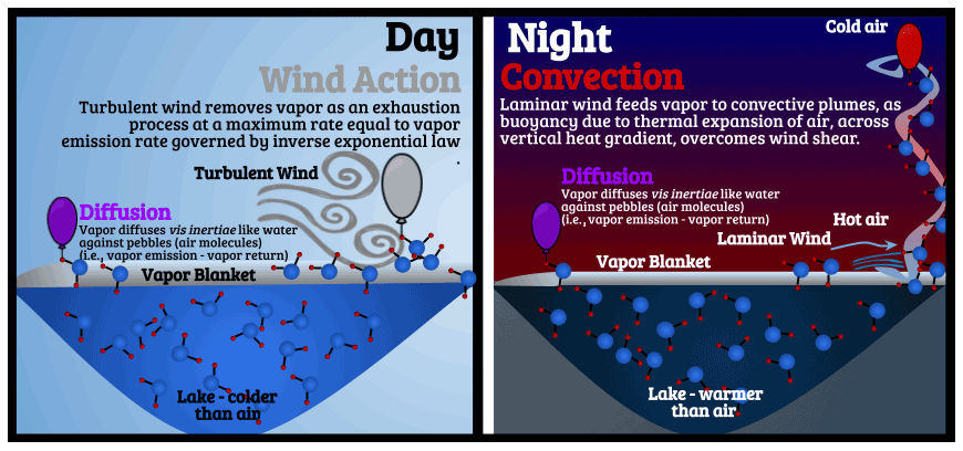
Here, the colored balloons represent evaporation aided by vapor removal due to diffusion (purple), wind action (gray), and convection (red). Diffusion can be upward or downward in direction, where upward (positive) is evaporation, and downward (negative) is condensation (see Sect. 3.5). The gray balloon (wind action) depends on the wind speed about 1 ft (0.3 m) away from the surface of the water, and it is governed by an inverse exponential law (see Sect. 3.2) and can happen during the day or night, though it is accentuated during the day when wind speed is higher. The red balloon (convection) depends on the temperature deficit across a vertical gradient and a laminar wind that accompanies vapor removal (see Sect. 3.2.3), and it occurs predominantly during the night (Horton, 1917a) when the water is warmer than air due to its higher heat memory (i.e., specific heat capacity).
In what follows, we illustrate Horton's evaporation equations, their theoretical basis (using direct quotes where possible), correction factors and tables (as parametric equations), and provisional values of coefficients with appropriate units.
3.1 Evaporation equations: pan evaporation, evaporative capacity, and lake evaporation
If Vw is the saturated vapor pressure (SVP) at the surface water temperature (θw) and va is the actual vapor pressure of the overlying air a small distance above the water surface at air temperature (θa), then the Dalton factor (more commonly called the vapor pressure deficit – VPD) is [Vw−va]. All evaporation equations use VPD, but in Horton's equation for evaporation, the VPD term is replaced with a variable VPD term (VVPD), [ΨVw−va], where the variable Ψ is called the wind factor (elaborated on in Sect. 3.2). Ψ is not to be confused with a constant factor as it varies with meteorological conditions and has no units. Its values range from 1–2 (), depending on the near-ground wind speed (w0), to account for vapor removal by wind action and convection from the vapor blanket (discussed in Sect. 3.2.4). There are multiple reasons behind the position of Ψ in VVPD, which can be inferred from Horton's (1917a, 1927, 1934) papers. We discuss these reasons in Sect. 3.2, with direct quotes from Horton, where appropriate, to convey his thinking.
Pan evaporation (EP) is used for first-order calculations, i.e., ignoring the sub-pan variability in evaporation (see. Sect. 3.4), which is the same as the evaporative capacity calculated using water surface temperature (ECw; Horton, 1927, p. 160) and is as follows:
C is a constant related to the time and elemental area over which evaporation happens and the units of measurement of evaporation and vapor pressure. Horton measured vapor pressure in inches of mercury and wind speed in miles per hour. Unless explicitly stated, for the purpose of illustration, these units will be used here. Metric equivalents are provided in the main text for equations where coefficients are introduced (also see Sect. E in the Supplement). The provisional values he prescribed for C (in inches per time units) are 0.4 for a small elemental area, 0.36 for a 12 square inch (77.4 cm2) pan over the daily scale, 12.2 for an average month of 30.42 d, and 73.2 for 6 months. Some of these provisional values for C are given in Horton (1917a) and others in Horton (1927). According to Horton (1917a), these values are not standardized and are subject to revision. We provide another provisional revised value for C in Sect. 3 (Table 3).
The evaporation capacity (EC), referred to air temperature when water and air temperature are at all times identical (e.g., in small lakes), is calculated with respect to the SVP of air (Va) as follows:
Horton defined EC as follows:
The maximum rate of evaporation which can be produced by a given atmospheric environment from a unit area of wet surface exposed parallel with the wind, the surface having at all times a temperature exactly equal to that of the surrounding air. (Horton, 1919a)
For small water bodies, particularly those with shallow depths, in the absence of water surface temperature data, when the lag between water and air temperature is negligible, Eq. (1b) can be used. Over pans, an area factor and the variability in the vapor blanket thickness should be taken into account (discussed in Sect. 3.3 and 3.4) but can be ignored over large lakes.
Lake evaporation (EL) is calculated (Horton, 1927, p. 160) with respect to the SVP of vapor blanket (Vb) as follows:
The SVP of the vapor blanket (Vb) is calculated from the corresponding vapor blanket temperature, θb (Horton, 1927, 161 pp.), using what is now called the Clausius–Clapeyron relationship, but in Horton's time this was calculated using graphical psychrometric charts (see Horton, 1921). The vapor blanket temperature is approximated by a simple relationship, , where Δ represents the difference between surface water and air temperature regardless of sign, i.e., , where θa is air temperature. The expression for θb appears to be only a heuristic (i.e., an approximation with no theoretical basis) that may be applicable only in monthly timescales. Furthermore, Horton (1927, 161–162) noted that it works for small variations of θw from θa but suggested that, if the air temperature is much higher than water when relative humidity approaches 100 %, then the relationship may not hold because, under such a condition, the distance over which the vapor blanket becomes fully formed approaches infinity (see Sect. 3.4).
3.2 Wind factor (Ψ)
The inclusion of Ψ in the VVPD terms is what leads Horton's equation to generalize across a variety of physical conditions and perform better than several other equations (see Sect. 4) and is what makes us consider Horton's evaporation formulae as semi-empirical or quasi-physical (or rational in Horton's terms; see Horton, 1941a).
The wind factor, Ψ, depends on the wind velocity close to the water surface (w0) which, when convection is ignored, is assumed to be of the form of an inverse exponential law, as follows:
In this paper, H is designated as the Horton lake evaporation constant. Horton assigned it a constant value of 2, but it could be a little lower (discussed in Sect. 4). For the value of k, a constant called the wind coefficient, Horton prescribes values of 0.2 or 0.3, depending on the exposure of the evaporation pan (Horton, 1917a), but our experiments (as will be shown later; see Table 3) show that it can be as low as 0.13. Apparently, the Ψ values change depending on the values assumed for k, and the Ψ tables Horton published (provided later as parametric equations in Sect. 3.2.4) are for k=0.3 (Horton, 1943b).
3.2.1 The adjustment of Ψ for convective vapor removal in light (or absent) wind
In the case where warm days are followed by cool nights, convective vapor removal may be important. Convective vapor removal happens more readily in the nighttimes than in the day times. When surface winds are suppressed by inversion, and when water temperature is higher than that of air, evaporation may be dominated by convection, so an alteration of the formula for Ψ given by Eq. (2a) is required. Horton's observations suggest that, for ordinary natural temperatures, the w0 in the exponent can be replaced by , which would then include the effect of convective transport in the absence of strong winds (given below as Eq. 2b). To calculate the combined convection and wind action when wind speed is low, conditions where convection prevails can be related to a Beaufort force scale for light or calm. Horton does not specify a threshold, but he prescribes 2 mi h−1 (0.89 m s−1) in an example problem. Therefore, when convection is not ignored, under mild winds, when θ>θa, Ψ under these conditions is given by the following:
where θ and θa are the temperatures (not to be confused with potential temperature) of water and air measured in Fahrenheit.
3.2.2 Theoretical basis of Ψ in relation to physically based methods
One familiar with the combined equation of Penman may recognize that Horton's approach to adjusting the wind term with a convective term bears some resemblance to the physics represented in the combined equation which uses a harmonic mean-like weighting, wherein the psychrometric constant accounts for the role of pressure (the aerodynamic term), and the slope of the saturation vapor pressure curve accounts for the role of temperature (the energetics term), together forming the combination method. Similarly, Horton's assumption that convection is caused by a combined effect of calm wind and temperature gradient appears to be logically related to part of the physics represented by the flux Richardson number (), i.e., the ratio of buoyancy production (B), which represents buoyant force from vertical temperature gradient (turbulent heat flux), to that of shear production (P), which is an aerodynamic term (momentum flux times wind velocity gradient). Refer to Stull (1988) and Hess (1979) for their derivations. Understanding these relationships may lead to improved formulations of Ψ.
3.2.3 Assumptions behind Ψ and rationale for its position in VVPD
Though the rationale behind Ψ was not discussed the first time Horton introduced his evaporation method (Horton, 1917a), in the context of applying his equation under varying conditions of pressure (elevation), in a paper 17 years later (Horton, 1934), Horton clarifies the main assumptions behind the usage of Ψ and the rationale for its position in VVPD, which can be summarized as the following four key points: (A) nonlinear control of wind, (B) wind as an exhaustion process, (C) the upper limit of wind's influence, and (D) wind's influence on condensation. As these are the main reasons for the superior performance of his method, we discuss them briefly in the following, with direct quotes where applicable.
- A.
Nonlinear control of wind. This assumption is motivated by a simple physical reason, which is apparently not considered elsewhere by the numerous other investigators who have studied evaporation by the mass transfer mechanism.
Most existing evaporation formulas are in error in that they involve a linear factor for wind correction such that wind effect apparently increases indefinitely as the wind velocity increases. It has been proved experimentally, and is indicated by physical considerations, that since the wind can do no more than to remove the water vapor as fast as it is emitted from the liquid surface, there is a maximum or limiting value of the wind factor corresponding to each water surface temperature. (Horton, 1917a)
Other investigators followed Dalton's (1802) suggestion and included a wind correction factor that assumes the form , where the wind velocity w is multiplied by a factor K. Furthermore, equations of this type do not account for Dalton's important observation that evaporation doubles with strong wind.
[…] with the same evaporating force, a strong wind will double the effect produced in a still atmosphere. (Dalton, 1802, 581–584)
The value of 2 for H in Ψ can, therefore, be credited to Dalton's (1802) experiments on evaporation, but it was also verified by Horton's own experiments with wind under varied conditions (Horton, 1917a).
- B.
Wind as an exhaustion process. To our knowledge, wind's role on vapor removal as an exhaustion process has not been studied by other investigators.
The removal of vapor by wind corresponds to a condition of natural exhaustion to which the inverse exponential law commonly applies. (Horton, 1917a)
The theoretical basis for such a view appears in some detail in Horton (1934), as follows:
Ψ [is] a wind-factor, based on the assumption that mechanical removal of vapor by the wind is of the nature of an exhaustion process and hence follows the inverse exponential or inverse compound interest law. It is also based on the assumption that the maximum possible effect of wind-action is to remove the newly emitted vapor from contiguity with the water-surface as fast as it is emitted. (Horton, 1934)
The natural exhaustion mentioned in the above quote is analogous to Horton's use of natural exhaustion in his paper on the physical interpretation of infiltration excess (see Horton, 1941a), where he explains that its physical basis can, in part, be justified from first principles, and such a use of the inverse exponential law is at least semi-rational (quasi-physical), as it gives a complete picture of the physical characteristics (in this case evaporation) under natural conditions. Based on the physics described by Horton, we infer that natural exhaustion happens from the reservoir (vapor blanket) of saturated vapor that is replenished by the vapor pressure of the water surface, which is then depleted by wind action and convection. Multiplying Ψ with the total vapor pressure deficit (or the vapor pressure of air) would not represent the same outcome. This point will become clearer in Sect. 3.5, where the constituents of the evaporation formula are discussed.
- C.
The upper limit of wind's influence. Horton provides a rational basis for the upper limit of Ψ in the following quote:
In accordance with the Dalton formula, with the form of wind factor hitherto commonly used, the rate of evaporation increases indefinitely as the wind velocity is increased. This is obviously incorrect, since the rate of evaporation cannot in any event exceed the rate of vapor emission, and the latter is not affected by wind velocity in the absence of waves and spray. There must be for each water-surface temperature a maximum rate of evaporation, which rate cannot be increased by further increase in the wind velocity. (Horton, 1917a)
The rationale for the wind factor can be understood by considering the extremes. Evaporation is at its maximum rate when wind speed is high (i.e., evaporation happens at double the rate as compared to still air, as Dalton observed), i.e., Ψ=2, then the formula for evaporation reduces to 2 CV, assuming v=0 (i.e., the air is fully dry), since we are interested in the extreme case. In the other extreme, if wind speed is 0, and humidity is high, then Ψ=1, so Horton's equation reduces to free diffusion in still air, similar to Dalton's (1802) equation, C(V−v).
The limitations of Dalton's (1802) evaporation work were well known before Horton's time. For example, it has been noted that Dalton's (1802) observations were for the month of August only, and the evaporation estimated using his equation was found to be imprecise in other summer months (Soldner, 1807). Quantifying the influence of wind on evaporation seems to have had some attention in a few other works, as evident from the following quote from Brutsaert (1982):
[Soldner's] perceptive remarks notwithstanding, during the next half century, apparently little progress was made as regards the effect of the air stream. […] Schübler's [1831] data obtained during 1826 at Tübingen […] showed that evaporation of a water surface exposed to wind was 1.7 times larger than that of a sheltered surface in summer, and 4 times larger in winter. (Brutsaert, 1982)
Nearly a century after Schübler, Kennedy (1933) revisited the topic. It appears that Horton was not aware of Kennedy's or Soldner's works; he seems to have relied solely on Dalton's observations.
- D.
Wind's influence on condensation. The position Ψ does not interfere with the extension to condensation. This is another distinct and physically meaningful aspect that differentiates it from other Dalton-type empirical equations. Horton conducted experiments to understand the role of wind on condensation, as suggested by the following quote:
Condensation or dew rarely occurs on windy nights […] experiments were made to determine the effect of wind on the condensation of moisture on the surface of cans containing ice and water, and mixtures of ice and salt. (Horton, 1917a)
In a paper 17 years later, Horton (1934) discussed the role of condensation, revisiting experimental results in conjunction with the properties of his equation, and he writes the following:
It is evident that wind – except a slight wind – does not affect the rate of vapor-emission and return by diffusion but it does increase the rate of mechanical removal of newly emitted vapor. Consequently it appears that wind tends to decrease condensation instead of increasing it. Horton (1934)
These observations agree with Rohwer's (1931) experiments, which Horton (1934) cross-checked. Kennedy (1933) observed that, when water is cooler than air, and for humidity above 77 %, condensation occurs under such (sub-adiabatic) conditions, and Horton's (1917a) argument (independent of Kennedy's) adds a different nuance in that condensation happens only under low wind speeds and decreases with increasing wind speed, which is captured with the formulation of Ψ.
3.2.4 Adjustment of Ψ for pan geometry
Horton felt quite strongly about improper usage of pan data.
The land-exposed evaporation pan appears to be about the poorest device humanly contrivable for the purpose of determining the evaporation losses from broad water surfaces. (Horton, 1917a)
But it is important to note that Horton did not advocate for not using pan data. The use of pan data as a proxy for lake evaporation is justified after due consideration of various factors that cause lake and pan evaporation to differ from each other, namely (1) humidity corrections, (2) rim height and depth effects, (3) vapor blanket formation and exhaustion characteristics governed by meteorological factors (wind speed), and (4) temperature difference between pan and lake surface (especially important in the case of large lakes). Used correctly, pan evaporation can be a good proxy or a validation to cross-check actual lake evaporation. The wind speed at ground level has to be corrected considering the pan diameter (D) and depth (d) below the rim and a factor . Pan evaporation is calculated as follows:
3.2.5 Values of Ψ and ground wind velocity
Horton (1927) conducted ingenious experiments on wind that circumvented the need for wind tunnels.
For the purpose of determining the effect of wind on evaporation, experiments were carried out at the author's laboratory, using pails filled close to the rim, and suspended so as to swing freely from a rotating frame. […] These experiments and studies served to determine the coefficients in the formula. (Horton, 1927)
Wind factor (Ψ) changes based on the wind speed measured near the ground (w0). Horton calculated w0 based on his and Stevenson's experiments for velocity variation by height (see Stevenson, 1882), but he only published the data in a report 10 years after the publication of his equation. The table provided by Horton (1927) for Ψ can be converted into a cubic polynomial with coefficients that have five decimal places for values of wind speed ranging from 0–15 mi/h (miles per hour) or, equivalently, 0–6.7 m/s (meters per second). For wind speeds beyond this limit, the value of Ψ can be linearly interpolated between 1.95 and 2 as a reasonable approximation. However, at near-ground level (at about 1 ft (0.3 m) height from the water surface), such speeds are quite unlikely. We believe that the main barrier in adopting Horton's equation widely was the lack of access to the wind correction tables in his lesser-known report (Horton, 1927), so we converted them into the following equations for convenience:
We also converted another table he provided in a much later work (Horton, 1943b) where the values for Ψ varied slightly, as follows:
The table values for Ψ might possibly be an error in Horton (1943b), but it seems worth pointing out the difference, however slight. To develop Eqs. (2d–f), we first extracted the values from Horton's table using online scanning software (https://extracttable.com/, last access: 18 January 2022), and then we fitted it as a two-parameter function with six unknowns (see the Supplement). We assessed several methods to develop parametric equations from Horton's tables, such as the monkey saddle, logarithmic and power law relationships, shifted divergence, rooting behaviors, etc., and were able to obtain a coefficient of determination of 0.99. However, the functions that provided this fit did not capture the high-velocity variations satisfactorily. We were fortunate to obtain an improved solution with the assistance of Nikolai Mikuszeit through stack overflow (see Vimal and Mikuszeit, 2021). The coefficient of determination (R2) of the best formulation was 0.999. Wind velocity, w0, is given by the following:
where wH and are the wind velocity in miles per hour and meters per second (metric) units, as measured by an anemometer at some height H (in feet) or Hm (in meters) above the ground or above the water surface. The equation holds for values of height of wind measurement and velocities, ft (60 m) and mi h−1 (48 km h−1), respectively. These values do not exceed typical conditions. To calculate wind measurements at heights other than w0, since algebraic manipulations cannot be easily used on Eq. (3b), a bisection search method was used to calculate wind velocities at various heights. We used this approach for deriving wind measurements at different heights. The bisection method converges to within two decimal places within 10 iterations and takes a fraction of a second, so it can be adopted for simulations over long time periods and over large domains with many grid cells.
3.2.6 Area factor for pan evaporation depending on turbulence and humidity
While using pan evaporation to calculate lake evaporation, an area factor is required (Horton, 1927, p. 162) to cross-check their respective values. The area factor, F, for pan evaporation uses the concept of evaporative capacity (Ecw) with respect to water temperature (note that the evaporative capacity in Eq. 1b is the same but with respect to air temperature, and Ecw is the same as EP given in Eq. 1a if the sub-pan variability is ignored and the surface temperature of pan and lake are the same). F is the ratio of evaporation from the lake EL to the evaporative capacity (Ecw) as follows:
When the water and air temperatures are identical (this would apply more for small lakes, where the temporal lag in water temperature is negligible), then Vw=Vb and va=hVw, where h is relative humidity given by .
If the air and water temperatures are equal, then the correction factor F reduces to the following:
Horton (1943b) deduced that when the air and water temperatures are not equal, then the area correction factor is related to two ratios (r and h′), where , and , as follows:
The influence of turbulence on F is discussed in Horton (1943a, b). If p is the fraction of time during which turbulent flow prevails up to some considerable height above the ground, under turbulent conditions, then the correction factor F is given by the following:
The derivation of Eq. (4d) is not shown step-by-step in Horton (1943a, b), but it appears that it follows directly from the following equation (Eq. 5) presented in Sect. 3.4, as indicated by the following quote from Horton:
[The author] deduced a rational expression for area-factor based on the assumption that near the windward edge of a broad water-surface an unknown fraction m of the emitted vapor is carried to leeward […] (Horton, 1943a, b)
Contemporary atmospheric boundary layer (ABL) theory helps approximate p, which can be determined to a fair degree of accuracy by estimating the diurnal variations in the boundary layer height (see Stull, 1988).
3.3 Vapor blanket characteristics
The vapor blanket is conceptually similar to a viscous sub-layer in open channel flow and is formed due to the existence of a laminar flow layer which horizontally transports moisture in the downwind direction, which leads to its growth in height. The horizontal variation in the vapor blanket height, which is of the order of a few meters, is critical when estimating pan evaporation. Pans have a poorly formed vapor blanket because of their small size, as even weak winds can remove the laminar layer before it is fully formed. Once pan evaporation is corrected for the formation and disturbance of the vapor blanket layer, their use for lake evaporation can be readily justified (Horton, 1927). In the case of both pans and lakes, the vapor blanket characteristics are the same (both are governed by meteorologic factors), but over pans the variation in evaporation over the variable thickness of vapor blanket is more important, while over large lakes they can be ignored as the area involved is small. It is important to account for the effect of the vapor blanket during both daytime (when it is slightly larger) and nighttime conditions (see the example problem in Horton, 1917a).
3.3.1 Horizontal variation in the vapor blanket
Understanding the process of vapor blanket formation and accurately quantifying its development and disturbance from the windward fringe of the lake to the leeward side can be considered as one of the main theoretical breakthroughs in Horton's evaporation work. The reason for it being an important breakthrough is that it explains why pans and large lakes have different evaporation rates. It provides a basis for ignoring the vapor blanket thickness variation in large lakes, and it explains why it would be a big mistake to ignore it from pans.
Horton derived an expression (see Eq. 5 below) to capture where, when, and how much the evaporation rate varies across the lake (or pan) surface. Assuming a strip of unit width, the horizontal distance of the vapor blanket before its thickness becomes constant (xc) is given by the following:
The horizontal scale of xc is typically of the order of a few yards. Our calculations show that it can be of the order of a few meters. υ0 is vapor pressure at the shore on the windward side, υc is vapor pressure at a distance x downwind, E0 is evaporation at the windward shore of the lake, Ec is evaporation at x, and m is the fraction of moisture carried by wind action from the shore towards the leeward side of the lake, where the vapor blanket thickness quickly approaches a constant value. Typical values of m are given as follows: 0 is water surfaces broken by waves and over rough land surfaces, 0.3–0.4 are for gusty winds; 0.6–0.7 are for steady winds, and 1 is a perfectly horizontal uniform wind (Horton, 1917a).
Though Horton does not provide the steps to derive Eq. (5), derivations for analogous problems which resemble this equation, as solved by Horton and others, may provide some insight. For convenience of reference, one such derivation by Horton (1927, p. 63) and how it can be interpreted for the derivation of Eq. (5) is given in the Supplement. Some examples of viscous sub-layer problems in open channel flow are given in Horton et al. (1936).
Another useful formula Horton provides is one for calculating evaporation (Ex) at any point x along the lake or pan. Assuming a strip with a unit width and length (x) downwind along the direction of the mean wind, evaporation at the point x is as follows:
Average evaporation (Eav) over the strip from shoreline to the location x over the developing vapor blanket is then the following:
3.3.2 Vapor blanket height
In most cases, the vapor blanket thickness is only a few millimeters, and it is related to wind velocity. Horton (1943b) presents an equation for the vapor blanket thickness given by Taylor and Shaw (1918). Though Horton's reference has the same title as that provided in reference, the year specified by Horton (i.e., 1934) could have been a typo, and the correct reference is likely to be the one given here. After inspecting Taylor's papers from 1934 and conducting a cursory search of his bibliography for similar titles, we did not find the equation Horton provided. From Horton (1943b), the vapor blanket thickness (Tg, in feet) given by Taylor is apparently Tg=0.0293w, where w is the wind speed at a height of 1 ft (0.3 m) in miles per hour.
Horton is among the few hydrologists to rigorously examine the role of the vapor blanket in lake evaporation. So, to conclude this section, a brief synopsis of some of the other studies conducted by other investigators may aid the readers in pursuing further research in this direction. Horton's source for the idea of vapor blanket and its contributions to evaporation rates could perhaps be the Slovenian scientist Jožef Štefan (1882).
The fact that the amount of evaporation from a basin is proportional not to the surface content but rather to the square root of this surface content leads to the result that evaporation from large water basins is proportionally smaller compared to the evaporation from a small basin. Let us also add that this is true not only for diffusion-driven evaporation but also for convection-driven evaporation. When an air current moves across a water surface, it will initially lift up large amounts of water vapor as soon as it crosses the boundary of the basin, but then it will not cause much evaporation as it progresses. (Štefan, 1882, p. 560; emphasis added; own translation)
A derivation similar to that of Eq. (5) is provided in an analogous problem of diffusion and evaporation by Štefan (1882), who may have inspired Horton's derivation. Štefan, in turn, relates the derivation to two other analogous problems in heat conduction and electricity. These analogous problems give the germ of the solution for Eq. (5). Mitrovic (2012) translated an important work conducted by Štefan, related to diffusion, that has been long forgotten.
The characteristics of the vapor blanket have been studied in only a few other works, to our knowledge. Sutton (1934) and Vercauteren (2011) have considered the shape of the vapor blanket in the windward edge, but its properties with respect to evaporation (and with regards to turbulence, convection, etc.) over lakes were not explored. Millar's (1937) apparently rigorous study of the vapor blanket was not accessible to us (we were unable to obtain a copy of the paper), but a summary is provided in a United States Geological Survey (USGS) report (1954; see the chapter on “Mass Transfer Studies” by Marciano and Harbeck), which shows Millar's equations. They indeed seem to resemble Štefan's work on diffusion. Finally, there is an indirect reference to the vapor blanket in Peter Eagleson's textbook on Dynamic Hydrology, which supposedly includes a description of the vapor blanket as a conceptual thin layer, and it is described with a schematic, but no sources were given (Eagleson, 1970; Fig. 12-1, p. 213).
3.4 Separable physical factors in the evaporation equation
3.4.1 Role of pressure (evaporation change with altitude)
To understand the role of vapor removal and diffusion, for convenience we can consider a general form of Eqs. (1) and (2). Ignoring convection, inserting Ψ from Eq. (2a) into Eq. (1a), the general (lake or pan) evaporation equation is given by the following:
If H, as given by Horton (drawn from Dalton), can be taken as a constant 2, then Eq. (8a) can be factored into the following:
By separating Eq. (8a) into its physically meaningful parts ,as shown in Eq. (8b), one can account for the role of barometric pressure which impacts only one of the terms (free diffusion, which is the first part here). When pressure changes with altitude, the first term here is adjusted for pressure drop. Horton's rationale is as follows:
It is evident that in order to determine the effect of change in barometric pressure on evaporation, other things equal, its effect on vapor removal by diffusion, which is always present, and its effect on vapor removal by wind-action, must be considered separately. This may readily be accomplished by the use of an evaporation formula published some years ago. (Horton, 1934)
An inverse relationship between diffusion and pressure was first proposed by Thomas Tate (1862) and later derived by Štefan (1882). If B0 and B are barometric pressures at datum (sea level) and pressure at a given elevation respectively, then the evaporation equation, according to Horton (1934), becomes the following:
The second part represents the enhanced vapor emission facilitated by vapor removal from the vapor blanket, which can be either by wind or convection; the wind's influence is independent of barometric pressure (Horton, 1934). The relationship between convection and barometric pressure was not known to Horton, and he had an argument to not investigate further.
The relation of barometric pressure to convective vapor removal has apparently not been studied. Since convection is, in general, not present when there is strong wind-action, it will not be considered here. (Horton, 1934)
Under humid conditions, Horton (1934) suggested that the role of wind-induced vapor removal may be several times higher than that of still air, but it does not appear that this effect is explicitly accounted for in his equation.
3.5 Experimental precision
The precision that went into Horton's experimental measurements is quite remarkable. He performed detailed experiments on the melting of snow, considering dozens of physical variables measured at 10–20 min intervals (Horton, 1915). These experiments and his earlier study on evaporation from snow (see Horton, 1914) resemble his later experiments on condensation (see Horton, 1917a). He designed his own instruments to measure minimum and maximum daily temperatures of water surface and a geometrical approach for snow temperature (Horton, 1919b). To cross-check his daily snow measurements, he made additional measurements at an accuracy of one-fifth of a degree at hourly intervals to cross-check the diurnal (min and max) daily snow temperature readings (Horton and Leach, 1934). He used graphical methods to calculate vapor pressure and humidity, which give values to within 1 %–2 % accuracy (Horton, 1921). Some evaporation measurements to cross-check his evaporation calculation (see Horton, 1927, 150–155) were made to approximately one-hundredth of an inch (0.00254 cm) precision.
4.1 Evaluating on an Arctic lake with observed and disaggregated vapor pressure
High-latitude lakes are quite important in the context of accelerated Arctic warming (Smith et al., 2005), as the region is besprinkled with numerous tiny lakes, where the mean evaporation for each lake may vary appreciably due to the variability in the vapor blanket thickness (Eqs. 5–8), which means that the role of the vapor blanket cannot be ignored. In the domain of Canada and Alaska alone, there are over 13 million lakes measured at Landsat resolution (∼0.1 ha but varies by latitude) and perhaps many more at finer scales. Horton (1934) noted that high-latitude evaporation processes may be quite different from midlatitudes because available water at the surface may be altered by condensation processes, and the predominant evaporation surface is snow, especially above the snow line (Horton, 1934). So it follows that the methods of midlatitudes cannot be directly applied, though Horton believed that his evaporation method is generalizable for sub-zero conditions and condensation (unlike the other empirical equations for evaporation).
Table 1Performance metrics (R2 and percent bias) for evaporation methods using observed data inputs. Darker shades of teal and pink highlight the good results. The time steps (units) are given as minutes, hours, days, weeks, and months.
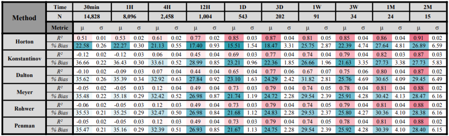
We tested Horton's evaporation equation on Baker Creek in subarctic Canada, where 30 min meteorological data were available as measured over the lake and near the lake (see Spence and Hedstrom, 2018, for the data description and measurement heights). For vapor pressures of air measured in either location, the difference in evaporation was slight. To evaluate the performance of Horton's equation, following Singh and Xu (1997), we selected five other equations that resemble Horton's equation, namely Konstantinov, Dalton, Meyer, Rohwer, and Penman. Note that the Penman equation referred to here is not the combined equation but only a part of the combined equation (aerodynamic) provided in Penman's original work (Penman, 1948). The general forms of the equations are given in Table 3 (Sect. 4.3). We calibrated each of them by treating all the coefficients as free parameters, preserving only the structure of the equation. Most empirical Dalton-type formulas do not include a temperature deficit term, except for a few that are of the type of Konstantinov (1968).
The actual vapor pressure of the air is one of the most important variables, but it is difficult to obtain. To understand how robust or how prone to error these methods are when it comes to this variable, in addition to using observed measurements available for the test site, we calculated actual vapor pressure as a function of solar geometry, diurnal temperature range, and seasonal precipitation (see Bennett et al., 2020 and Bohn et al., 2013). The data for this calculation were drawn from our previous work (Vimal et al., 2019).
We used a bootstrap approach to obtain the mean (μ) and standard deviation (σ) for the coefficient of determination (R2) and percentage bias (percent of mean absolute percentage error), where we sampled 50 %, 75 %, and 100 % of the record length, 50 random samples with a replacement for each length, and 11 timescales (30 min to 2 months), leading to a total of 1650 random bootstrap samples. For all these combinations, the time period of analysis was 8 April 2009 to 20 September 2016. Missing values were ignored, and the data coverage mostly represents summer months (further details are in Spence and Hedstrom, 2018).
Table 1 shows that Horton's method is substantially more accurate than the other methods, and this is seen consistently across timescales and sample sizes. This seems to also be true when considering other classes of models (radiation based, temperature based, or a combination), as evidenced by relative performances reported in Tan et al. (2007). The only exception seems to be artificial neural network (ANN) models, which appear to have the potential to be marginally superior to Horton's, going by their relative performance, but they require sufficient site-specific data and tuning.
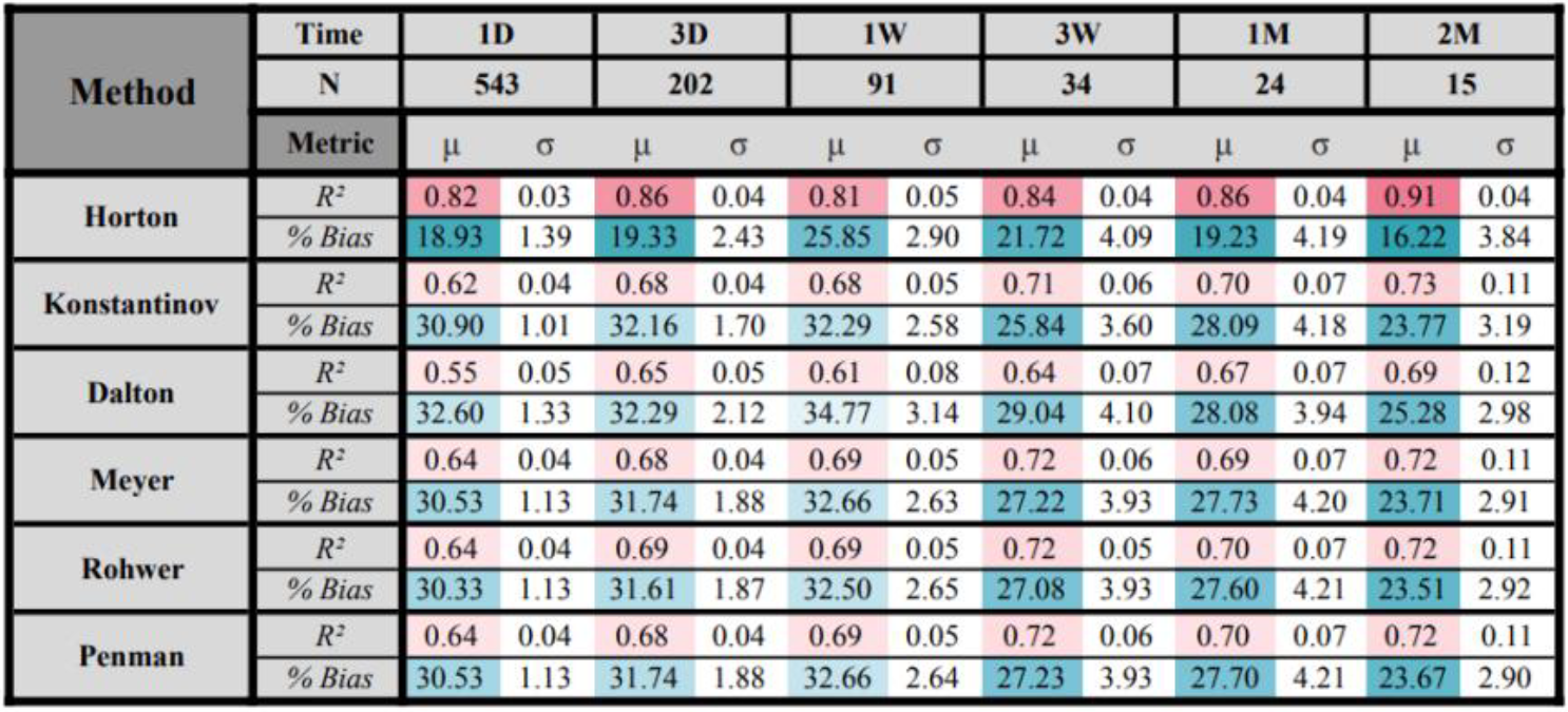
Surprisingly, Horton's method outperforms other methods, even when using the estimated input vapor pressure (Table 2) and even if the results of Horton's equation from Table 2 (estimated actual vapor pressure) are compared with the five methods from Table 1 (local measurements). It must be noted that previous studies have shown that vapor pressure near water bodies (e.g., coastal regions) has a large bias and uncertainty (see Bohn et al., 2013), which makes the result even more surprising. A reason for the poorer performance of other methods could be that we estimated wind velocity at various heights by back-calculating, using Eq. (3b), and the bisection method previously mentioned (Sect. 3.2). Another reason could be the dependence of the vapor pressure measurement on the observation height for some, even if not all, of the other methods. Konstantinov's equation depends on wind speed at ground height (which is same as Horton's method), and uses more input variables related to temperature, and yet does not perform better. We do not draw bald conclusions directly from Tables 1 and 2 before testing under multiple catchments and lakes of wide-ranging meteorological conditions. However, if this result holds across various locations and regions, as we will show in Sect. 4.5 more generally, then, taken together, we can arrive at a few conclusions. (1) Horton's formula is robust against over-fitting of errors, making it more physically based. (2) The variable vapor pressure deficit (VVPD) term, unique to Horton's evaporation formula, is a better control on evaporation than VPD.
Table 2Performance metrics (R2 and percent bias) for evaporation methods using reanalysis-based disaggregated actual vapor pressure. Darker shades of teal and pink highlight good results. The time series (units) are given as days, weeks, and months.
4.2 Generality of the method
We use the term generality to mean the following connotations: (1) parameter certainty, i.e., how relatively unchanging the parameters in the calibrated equations are across wide-ranging conditions, time averages (the mean of evaporation is considered when time averaging, so the effect of time in parameters is ignored), and record lengths; (2) how well it performs in wide-ranging conditions across various meteorological conditions and altitudes; and (3) how well it performs over continental scales, which follows from both (1) and (2). The ability of a method to generalize across such conditions shows that the method is not an empirical fit but has a rational or physical basis.
4.3 Parameter certainty
If the parameter values are unchanging or have only a slight variability, then they can be assumed to possess a physical meaning which does not need site-specific tuning (or calibration). Such unchanging values are termed constants, and identifying such constants is common in physics. Of the three connotations of generality we are interested in, parameter certainty is the most important. In all the six methods we compared, there were 17 parameters, and each one was tuned for each of the 1650 bootstrapped samples, using a vectorized approach (see Sect. 4.1 for a breakdown of the sample size and record lengths). The tuned parameters are summarized in Table 3 (shown below). To make their comparison straightforward, the time unit of reference observation was kept identical to the native resolution, e.g., daily or monthly evaporation values were averaged into units of millimeters per 30 min, which allows us to compare values of parameters across methods and timescales. Some outliers in the parameter values were found (possibly due to errors in the data) but were removed using the same criteria (10th percentile) for all six methods each considered independently. The last column here shows normalized values of variability () as a percentage, which can be compared across methods.
Table 3Parameter uncertainty comparison between six evaporation formulas (mean μ and ).

Among all the parameters, parameter H has the most unchanging value (1.71) and the smallest (1.3 %) relative variability ( %), while average of all the other parameters is 9.5 %, which shows that it is the most generalizable and requires the least site-specific tuning among the 17 parameters considered across all six methods. The value for H that Horton originally prescribed was 2, drawing from Dalton's experiments (see the quote in Sect. 2.2.2). The other two parameters of Horton's equation are not particularly more certain than the parameters of other equations. Meyer's equation, which relies on wind speed at 9 m height, has one of the parameters (C) that performs nearly as well as Horton's H, with 1.6 % variability.
Previous investigations on H
To our knowledge, there is no other evaporation formulation that captures the role of H, though aspects of its role have been observed previously. Horton's source for H could be regarded as Dalton (1802). Dalton conducted his experiments in a single site in high and low evaporation conditions and high and low temperatures, so our result (1.71) can be said to be more robust than Dalton's, as our bootstrap sampling strategy accounts for more wide-ranging conditions. Even so, the value of 1.71 may need confirmation from several lakes across latitudes to ascertain its value. This value, interestingly, agrees very closely with Schübler's (1831) experimental observations that evaporation accentuated by wind during summer was 1.7 times greater (Brutsaert, 1982). The parameter H appears to be a significant development in lake evaporation physics and can be designated as the Horton constant, sharing credit with Dalton and Schübler.
4.4 Estimates across altitudes and sub-zero temperature conditions
Horton claimed that his method was rational (physical) in that it is robust to conditions outside of which it was used (Horton, 1927, p. 159), which the other empirical methods of his time were not (e.g., the method by Carpenter and Fitzgerald; see Fitzgerald, 1886), as most were tuned for local conditions. Horton investigated the role of condensation rates, evaporation from snow surfaces (Horton, 1914), temperature deficits, and wind speed in high altitude and polar regions (Horton 1934). In a Central Snow Conference paper (Horton, 1941b), he comments on the processes involved in evaporation from snow that includes independent variables that depend on latitude and altitude, which were not known with certainty. When lake surfaces are partially covered with ice, he recommends using a weighted average of lake water and ice temperatures for partially frozen lakes. The role of the thickness of ice on the air–water temperature relationship was observed, i.e., thicker ice brings the air and water temperature closer. Additional factors that influence evaporation under such conditions could be the percentage, intensity, and duration of laminar and turbulent air flow, which depend on latitude and elevation (Horton, 1943a, b), and also other physical factors due to snow and ice, that is, (A) the area exposed to air (vs. projected area from snow surface) due to the influence of snow porosity may increase evaporation and (B) the disproportionate distance of air temperature from ice temperature (as opposed to water temperature). Horton (1934) suggested that these additional factors may require a separate treatment.
4.5 Evaluating Horton's evaporation results over the continental U.S.
Horton used the data of 112 pan evaporimeters over the continental U.S. and plotted precipitation, evaporation, and runoff into one figure sliced by longitudes (see the figure in Horton, 1943a, b). We replotted his chart together with land surface model results simulated at over 200 000 model grid locations over the continental U.S. by Livneh et al. (2013). We aggregated the model results in the same way as Horton did by 2∘ grid boxes. Surprisingly, the curves for P, E, and Q are remarkably similar (see Fig. 2). We further aggregated the data into three climate normals, i.e., three 30-year averages from 1921 to 2010 to see whether there exist long-term climate change influences, but we found none. This could possibly be an inherent issue with the Livneh et al. (2013) dataset, which possibly is detrended. The record lengths of Horton's data were variable, so they are not shown, but they are of the order of magnitude to be regarded as climate normals, i.e., a long-term climate average.

Figure 2Comparison of continental U.S. 2∘ average values of precipitation (P), evapotranspiration (E), and runoff (Q) estimates. We replotted the chart from Horton (1943b) together with Livneh et al. (2013) over three climate normals.
The difference in evaporation is substantial in the Great Lakes region (between longitudes of −90 and −80), though the precipitation seems to be similar, and this may be explained as follows. Cleveland and Chicago, which are on different sides of the Great Lakes, may have a similar temperature (except in winter), but the number of sunshine hours (and cloud cover) may change significantly between the two places (see Jensen and Haise, 1963). Some of these factors were directly and indirectly accounted for in Horton's estimation of evaporation from the Great Lakes. For example, he considered wind data from multiple locations and performed some interpolation-based corrections. Also, the land surface model results were masked out for the Great Lakes pixels, so it is possible that the evapotranspiration of that longitude band, on average, is greater than the evaporation from Great Lakes, which may explain the difference. Larger lakes, as noted by Štefan (1882) and suggested by Horton's formula (Eq. 5), may possibly yield a lower total evaporation than the rest of the land surface, which is quite nonintuitive, but for the scale of the Great Lakes, this cannot be ascertained as there may be numerous other factors that come into play. However, we can conclude that the evaporation formula does generalize over continental scales owing to the remarkable similarity seen in Fig. 2.
5.1 Horton's contribution to lake evaporation physics
While this paper highlights a century-old method, we do not fail to recognize that advancements in evaporation theories of the last century have been stellar. One needs to only look at the number of numbers (mostly dimensionless) that are used to represent the physics that control evaporation, including Dalton, Reynolds, Prandtl, Taylor, Karman, Stanton, Schmidt, (flux) Richardson, Péclet, Nusselt, Sherwood, and Raleigh (see Pasquill, 1942, Hess, 1979, and Brutsaert, 1982, for an introduction to many of these developments). Besides the fields of aero-, thermo- and hydrodynamics, where most of these numbers emerged, there have been also great strides forward in the kinetic theories of evaporation (see Gerasimov and Yurin, 2018). One can argue that progress would lead to the unification of these numbers into a smaller set. Nevertheless, in the quest for the smaller set, among the candidate numbers, we believe two of Horton's core contributions discussed in this paper could be considered for their fundamental relevance to lake evaporation estimation. (1) The ratio in Eq. (5), which represents the ratio of evaporation at the fringe of the lake to evaporation where the vapor blanket acquires a constant thickness, and (2) H, the seemingly constant coefficient (see Table 3), the value of which was prescribed by Horton as 2 (or a little lower, as we find, at 1.7), which is arguably what makes the VVPD term a better independent control on evaporation than VPD. These two points, we suggest, could be called the Horton ratio and the Horton constant for lake evaporation, respectively. The former could also be credited to Štefan (1882); see also Mitrovic (2012), who rediscovered another century-old problem credited to Štefan, and the latter to John Dalton (1802) and Gustav Schübler (1831). It appears that Horton provided the first quantitative treatment highlighting the importance of these two values for lakes.
5.2 Can Horton's evaporation formula replace other methods?
Among the five equations we evaluated, Meyer's, Rohwer's, and Penman's equation shapes and results differ but only slightly. Expectedly, Konstantinov's (1968) method, which draws additional information from a temperature-deficit term, in addition to VPD and wind (as done in other methods), has the second-highest complexity and performs the second best, while Dalton's method (the simplest one) is the poorest. What we have shown here suggests that Horton's equation can indeed replace these other methods. A question that begs to be answered here is whether Horton's evaporation equation for lakes should be preferred over the Penman (combination) equation, especially in the context of continental-scale land surface modeling? Before answering this question, it is worth noting that Penman's formula is, in part, adapted from Rohwer's (1931) formula, who, in turn, in his work commented on Horton's evaporation formula, saying the following:
From a theoretical standpoint [Horton's] formula is worthy of consideration, but, as the values of the constants in the formula have not been definitely determined, the practical value of the formula is small. (Rohwer, 1931)
Our answer to this question from this study is that it could be for the following reasons.
- 1.
Horton's VVPD can replace VPD. The aerodynamic part of the Penman equation invariably depends on the VPD term which, as we showed in Sect. 4.1, will indeed be less accurate than Horton's VVPD.
- 2.
Separability of barometric pressure. The Penman aerodynamic component is weighted by a psychrometric constant (essentially a barometric pressure term), which plays a role in diffusion but not aerodynamic action. As shown in Eq. (8c), an inverse barometric pressure term may be added to only the diffusion term, which is separable from wind action, which is possible with Horton's equation but not with the other aerodynamic formulas hitherto used in various combination methods (e.g., Penman and others).
- 3.
Error in energy variables. The energy balance approach relies on variables such as surface radiation and ground heat flux (which depend on cloud cover, ground heat exchange, etc.), which are prone to errors. Furthermore, there exist first-order issues with energy budgets because of errors in a crucial variable, open water albedo, which varies as a function of the Sun's angle (see the field experiments by Sivkov, 1971). Seasonal variability can be up to a factor of 7, but most lake schemes do not account for this variability; for example, the lake energy scheme of Bowling and Lettenmaier (2009) uses a constant albedo value for open water (similarly in Hostetler and Bartlein, 1990; and Croley, 2012).
- 4.
Horton's method depends on water temperature data and not radiation. Using water surface temperature data for evaporation has the crucial advantage that it can be directly measured from space (see Sharma et al., 2015), especially for large water bodies, with a fair degree of accuracy (∼1.15 ∘C for small lakes and 0.45 ∘C for large lakes). Rapid mixing of surface water due to wind and vertical density gradients (see the experiments on stratification by Gregory, 2012) together favor the surface water temperature to equalize quickly across the surface. This is especially true in small lakes where surface temperature can be considered as uniform. Over large lakes, the temperature varies with bathymetry due to variable rates of vertical mixing. However, this variability only depends on lake bathymetry which can be treated as a static parameter, and heat exchange can be modeled or observed with better accuracy in larger lakes from space observations (as noted before). On the other hand, in a study by Rahaghi et al. (2019), it was shown that radiation at the surface of a large Swiss lake (Lake Geneva) varied of the order of greater than 40 W m−2 in different parts of the same lake, which is quite a significant error for a large lake, and was attributed to shading effect by clouds, which is a dynamic error. In terrestrial hydrology, where the radiation budget is calculated from temperature (e.g., Bohn et al., 2013), Horton's method has a particular advantage. These arguments make a strong case for favoring Horton's equation over the combination method for both large and small lakes.
5.3 Should we revisit the evaporation paradox?
The relationship between pan and actual evaporation is a topic of great importance today in the wake of accelerated climate warming. There is unanimous consensus that pan evaporation is reducing globally, while in a warming climate the opposite is generally expected, which is known as the evaporation paradox (Roderick and Farquhar, 2002). A friendly introduction to the topic is given in Singh (2016; see Sect. 42.2.3). This paradox is explained by evaporation observations in larger scales across sites of variable moisture availability, considering how energy is redistributed between latent and sensible heat based on moisture availability. This paradox is considered to be resolved by Bouchet's (1963) principle of complementarity, which shows the relationship between pan, actual, and theoretical evaporation. Morton (1994), Szilagyi et al. (2017), Brutsaert and Yeh (1970), and Brutsaert (1982, 2015) further extended the work by Bouchet (1963). In studies that involve pans, including several that are related to the evaporation paradox, pan evaporation calculations are often done with a static pan correction parameter, but as Horton expressed very clearly (see the quote in Sect. 3.2.2), it would be quite wrong to use a simple, static pan correction parameter (Horton, 1917a). The explicit role of the vapor blanket has been ignored in these studies, except perhaps indirectly (as moisture availability is related to atmospheric humidity, which influences vapor blanket characteristics). A table in Maidment (1992; Table 4.3.1; see Sect. 4 on “Evaporation” by Shuttleworth) taken from Doorenbos and Pruitt (1977) provides a quasi-quantitative guidance on pan correction as a function of humidity values and a scale similar to the Beaufort wind force scale (i.e., light, moderate, and strong winds). However, Horton's quantitative treatment and physical explanations for the differences in evaporation rates from the pan to lake precedes Doorenbos and Pruitt (1977) by half a century and is more nuanced and rational (i.e., has a strong physical basis) and is quantitative. Furthermore, Horton's insights on the vapor blanket's physical properties (Sect. 3.4) and the area factor, F (Sect. 3.3), shed new light on the evaporation paradox and generalizes it beyond standard pan sizes. Considering these points, it seems that a revisit to explain the evaporation paradox is warranted.
Horton's century-long forgotten works on lake evaporation seem to have great contemporary value for the theoretical insights they offer and for their relevance in modeling lakes of all sizes. The fine-scale precision afforded by Horton's law-of-the-wall-type equation (Eq. 5) and Eqs. (6) and (7) for the vapor blanket characteristics, credited to Jožef Štefan and Horton, appear to be essential to estimate the evaporation in small lakes and pans and using pan evaporation as a proxy for large lakes. From these equations, considering the importance of the Horton ratio (), taken together with the area factor F (Eq. 4a–d) for pan evaporimeter measurements, an opportunity arises to revisit the complementarity relationship between pan and lake evaporation and the so-called evaporation paradox. More generally, Horton's improved formulation that relies on the Horton constant H and VVPD (credited to John Dalton, Gustav Schübler and Horton), due to the dynamic wind factor Ψ (Eq. 2a–c), may partially or fully supplant other evaporation equations that rely on VPD, owing to its better generalizability (local to continental and across timescales and latitudes). We believe that Horton's evaporation method was largely overlooked and forgotten because the tables needed for their proper use were unavailable widely. Therefore, in this paper, we present the parametric forms of his ground wind velocity experimental results (Eqs. 2d–f and 3b), which may serve as a ground reference for a wider use of his method. Considering all of this, our main conclusion is that Horton's (1917a) claim of having developed a superior evaporation method (Eq. 1a–c) has as yet not been fully understood or proven wrong in a little over a century, and it appears to provide new directions to understand evaporation physics for contemporary climate-change-era problems.
As a closing note, to entertain the History of Hydrology Special Issue readers, we would like to highlight an amusing historical anecdote that came out of Horton's detailed evaporation study. In the early morning, over warm lakes in a cold climate, when the wind is calm and a laminar flow of wind on the surface of the lake feeds the moisture into convective plumes of vapor, they appear as columns of about 10 in. (25 cm) in diameter and over 4 ft (1.2 m) in height (a bit taller sometimes). Horton had the rare chance to witness these apparitions in his early morning observations (he calls them the dancing columnar vapor drift; Horton, 1933). He notes that this phenomenon, as also previously noted by a German scientist (Johannes Walther), may be a curious explanation of the origin myth of the Greek deity Venus and that of the dancing Nereids upon Greek waters.
We hope that the various observations and conclusions drawn here to highlight the value of Horton's lake evaporation works will be developed further. We also hope that this serves to rekindle the interest of readers in (re-)discovering Horton's contributions to lake evaporation, in addition to his broader published and unpublished works.
The data sets used in this article are publicly available (see Sects. 1, 3.2.3, 4.1, and 4.5), and the codes are available upon request to the corresponding author. Horton's updated bibliography (with full references and notes) is available upon request to the corresponding author. Titles and years of the same are provided in the Supplement.
The supplement related to this article is available online at: https://doi.org/10.5194/hess-26-445-2022-supplement.
SV conceptualized the study, performed simulations, and prepared the paper. VPS conducted the literature search, designed the simulations, interpreted Horton's derivations, and edited the paper.
The contact author has declared that neither they nor their co-author have any competing interests.
Publisher's note: Copernicus Publications remains neutral with regard to jurisdictional claims in published maps and institutional affiliations.
This article is part of the special issue “History of hydrology” (HESS/HGSS inter-journal SI). It is not associated with a conference.
The authors would like to acknowledge the following individuals: (1) Anna Bonazzi, from the UCLA Germanic Languages department, for the translation of a German text (Štefan, 1882) cited here, for proofreading, and for sharing some ideas which improved this work; (2) Elizabeth Clark (formerly at UCLA), for inspiring Fig. 2 and for sharing her collection of 135 of Horton's titles; (3) Eric Sheppard, UCLA, for inspiring the work on scientific knowledge production in a graduate class and also for providing numerous comments on a broader version of this work; (4) Nikolai Mikuszeit (see Vimal and Mikuszeit, 2021), who offered his feedback via stack overflow and provided a superior solution for Horton's wind velocity height correction; (5) Keith Beven, Lancaster University, handling Editor, who provided numerous comments to improve the paper; (6) Dennis Lettenmaier, UCLA, for sharing some interesting perspectives and articles by Horton.
This paper was edited by Keith Beven and reviewed by Thomas McMahon and Adriaan J. (Ryan) Teuling.
Accavitti, J.: Robert E. Horton Papers. Finding aid with Archivists' Toolkit, available at: https://library.albion.edu/sites/default/files/Robert E. Horton papers.pdf, last access: 13 August 2019.
Bennett, A. R., Hamman, J. J., and Nijssen, B.: MetSim: A Python package for estimation and disaggregation of meteorological data, J. Open Source Softw., 5, 2042, https://doi.org/10.21105/joss.02042, 2020.
Bernard, M.: Appendix B – A review of “A new method of estimating stream-flow” by J. A. Folse, Eos Trans. Am. Geophys. Union, 17, 309–312, https://doi.org/10.1029/TR017i002p00309, 1936.
Beven, K.: Infiltration excess at the Horton Hydrology Laboratory (or not?), J. Hydrol., 293, 219–234, https://doi.org/10.1016/j.jhydrol.2004.02.001, 2004a.
Beven, K.: Robert E. Horton and abrupt rises of ground water, Hydrol. Process., 18, 3687–3696, https://doi.org/10.1002/hyp.5741, 2004b.
Beven, K.: Robert E. Horton's perceptual model of infiltration processes, Hydrological Processes, Wiley Online Library, available at: https://onlinelibrary.wiley.com/doi/pdf/10.1002/hyp (last access: 12 December 2021), 2004c.
Bohn, T. J., Livneh, B., Oyler, J. W., Running, S. W., Nijssen, B., and Lettenmaier, D. P.: Global evaluation of MTCLIM and related algorithms for forcing of ecological and hydrological models, Agr. Forest Meteorol., 176, 38–49, https://doi.org/10.1016/j.agrformet.2013.03.003, 2013.
Bouchet, R. J.: Evapotranspiration Réelle et Potentielle, Signification Climatique, IAHS Publ., 62, 134–142, 1963.
Bowen, I. S.: The Ratio of Heat Losses by Conduction and by Evaporation from any Water Surface, Phys. Rev., 27, 779–787, https://doi.org/10.1103/PhysRev.27.779, 1926.
Bowling, L. C. and Lettenmaier, D. P.: Modeling the Effects of Lakes and Wetlands on the Water Balance of Arctic Environments, J. Hydrometeorol., 11, 276–295, https://doi.org/10.1175/2009JHM1084.1, 2009.
Brutsaert, W.: Evaporation into the Atmosphere: Theory, History and Applications, Springer Netherlands, https://doi.org/10.1007/978-94-017-1497-6, 1982.
Brutsaert, W.: A generalized complementary principle with physical constraints for land-surface evaporation, Water Resour. Res., 51, 8087–8093, https://doi.org/10.1002/2015WR017720, 2015.
Brutsaert, W. and Yeh, G.-T.: Implications of a Type of Empirical Evaporation Formula for Lakes and Pans, Water Resour. Res., 6, 1202–1208, https://doi.org/10.1029/WR006i004p01202, 1970.
Chow, V. T.: Handbook of Applied Hydrology: A Compendium of Water-resources Technology, McGraw-Hill, https://doi.org/10.1080/02626666509493376, 1964.
Croley, I. I.: Recent Great Lakes Evaporation Model Estimates, 1–11, https://doi.org/10.1061/40792(173)551, 2012.
Dalton. J.: Experimental Essays on the Constitution of Mixed Gases; on the Force of Steam or Vapor from Water and Other Liquids in Different Temperatures, Both in a Torricellian Vacuum and in Air; on evaporation and on the expansion of gases by heat, Mem. Manchester Lit. Philos. Soc., 5–11, 535–602, 1802.
Davidson, P. A., Kaneda, Y., Moffatt, K., and Sreenivasan, K. R. (Eds.): A Voyage Through Turbulence, Cambridge University Press, Cambridge, ISBN 9781139502047, 1139502042, 2011.
Dolbear, A. E.: Matter, Ether, and Motion: The Factors and Relations of Physical Science, Lee and Shepard, available at: https://www.google.com/books/edition/Matter_Ether_and_Motion/Tfw4AAAAMAAJ?hl=en&gbpv=1&pg=PP1&printsec=frontcover (last access: 12 December 2021), 1892.
Doorenbos, J. and Pruitt, O. W.: Crop water requirements, Irrig. Drainage Pap. 24,Food and Agriculture Organization, Rome, available at: https://www.fao.org/3/f2430e/f2430e.pdf (last access: 12 December 2021), 1977.
Eagleson, P. S.: Dynamic Hydrology, McGraw-Hill, ISBN 9780070185968, 1970.
Fitzgerald, D.: Evaporation, Van Nostrand's Engineering Magazine (1879–1886) 35, 41–43, available at: https://search.proquest.com/docview/738662541/abstract/12D551E549C4EFDPQ/1 (last access: 12 December 2021), 1886.
Folse, J. A.: A new method of estimating stream-flow, based upon a new evaporation formula, Washington, Carnegie Institute of Washington, 302 pp., 1929.
Foufoula-Georgiou, E.: VHP Scope – Hydrology, available at: https://connect.agu.org/hydrology/vhp-scope/roberthorton, last access: 21 May 2021.
Gerasimov, D. N. and Yurin, E. I.: Kinetics of evaporation, Springer, ISBN 9783319963037, 2018.
Gregory, S.: Lake stratification with Stan Gregory, Videos 1 and 2, Oregon State University Ecampus, available at: https://www.youtube.com/watch?v=XExQ6uaDEJQ (last access: 8 May 2021), 2012.
Hall, F. R.: Contributions of Robert E. Horton, History of Geophysics, Vol. 3, AGU – American Geophysical Union, 113–117, https://doi.org/10.1029/HG003p0113, 1987.
Hess, S. L.: Introduction to Theoretical Meteorology, R. E. Krieger Publishing Company, ISBN 0882758578, 1979.
Horton, R. E.: The Drainage of Ponds into Drilled Wells, US Geological Survey Water-Supply Paper 145, available at: https://catalog.hathitrust.org/api/volumes/oclc/13028128.html (last access: 12 December 2021), 1905.
Horton, R. E.: Evaporation from Snow and Errors of Rain Gage When Used to Catch Snowfall, Mon. Weather Rev., 42, 99–100, https://doi.org/10.1175/1520-0493(1914)42<99:EFSAEO>2.0.CO;2, 1914.
Horton, R. E.: The Melting of Snow, Mon. Weather Re., 43, 599–605, https://doi.org/10.1175/1520-0493(1915)43<599:TMOS>2.0.CO;2, 1915.
Horton, R. E.: A New Evaporation Formula Developed, Engineering News-Record, 78, 196–199, 1917a.
Horton, R. E.: Failure of Hydraulic Projects from Lack of Water Prevented by Better Hydrology: More Complete Study of Stream Yield Is First Step – Low-Flow Frequency, Degree of Flashiness and Dry-Weather Evaporation Cannot Be Neglected, Engineering News-Record, 78, 490–492, 1917b.
Horton, R. E.: Drainage-Basin and Crop Studies Aid Water-Supply Estimates: Survey of Culture and Soil Will Lead to Estimates of Losses by Plant Interception and Transpiration and by Soil Evaporation – Most of the Evaporation Formulas now Used Are in Error, Engineering News-Record, 79, 357–360, 1917c.
Horton, R. E.: Rainfall Interception, Mon. Weather Rev., 47, 603–623, https://doi.org/10.1175/1520-0493(1919)47<603:RI>2.0.CO;2, 1919a.
Horton, R. E.: Device for Obtaining Maximum and Minimum Water Surface Temperatures, Mon. Weather Rev., 47, 856–857, https://doi.org/10.1175/1520-0493(1919)47<856c:DFOMAM>2.0.CO;2, 1919b.
Horton, R. E.: Vapor Pressure and Humidity Diagram, Mon. Weather Rev., 49, 285–287, https://doi.org/10.1175/1520-0493(1921)49<285:VPAHD>2.0.CO;2, 1921.
Horton, R. E.: Hydrology of the Great Lakes, Sanitary District of Chicago, available at: https://www.worldcat.org/title/hydrology-of-the-great-lakes-report-of-the-engineering-board-of-review-of-the-sanitary-district-of-chicago-on-the-lake-lowering-controversyand-a-program-of-remedial-measures-part-iii-appendix-ii/oclc/42987071&referer=brief_results (last access: 12 December 2021), 1927.
Horton, R. E.: Columnar Vapor Drift, B. Am. Meteorol. Soc., 14, 238–240, 1933.
Horton, R. E.: Water-Losses in High Latitudes and at High Elevations, Eos Trans. Am. Geophys. Union, 15, 351–379, https://doi.org/10.1029/TR015i002p00351, 1934.
Horton, R. E.: Apples From Eden and Other Short Stories, Christopher Publishing House, available at: https://www.worldcat.org/title/apples-from-eden-and-other-stories/oclc/9094396&referer=brief_results (last access: 12 December 2021), 1938.
Horton, R. E.: An Approach Toward a Physical Interpretation of Infiltration-Capacity 1, Soil Sci. Soc. Am. J., 5, 399–417, https://doi.org/10.2136/sssaj1941.036159950005000C0075x, 1941a.
Horton, R.: The Role of Snow, Ice and Frost in the Hydrological Cycle, in: Central Snow Conference, 11–12 December 1941, East Lansing, Michigan, 5–21, 1941b.
Horton, R. E.: Evaporation-Maps of the United States, Eos Trans. Am. Geophys. Union, 24, 743–753, https://doi.org/10.1029/TR024i002p00743, 1943a.
Horton, R. E.: Hydrologic Interrelations between Lands and Oceans, Eos Trans. Am. Geophys. Union, 24, 753–764, https://doi.org/10.1029/TR024i002p00753, 1943b.
Horton, R. E.: Report on Proposed Improvement and Extension of Hemlock Lake Water System, available at: http://www.wemett.net/hemlock/reservoir/reservoir_contents.html (last access: 1 May 2020), 1944.
Horton, R. E. and Leach, H. R.: Snow-surface Temperature, Mon. Weather Rev., 62, 128–130, https://doi.org/10.1175/1520-0493(1934)62<128:ST>2.0.CO;2, 1934.
Horton, R. E., Eaton H. N., Leighly, J., Smith, J. R., and Saville, T.: Relation of Hydraulic and Laboratory Research to Physical and Economic Geography, Impr. des caisses d'épargne, available at: http://hydrologie.org/ (last access: 19 April 2021), 1936.
Hostetler, S. W. and Bartlein, P. J.: Simulation of Lake Evaporation with Application to Modeling Lake Level Variations of Harney-Malheur Lake, Oregon, Water Resour. Res., 26, 2603–2612, https://doi.org/10.1029/WR026i010p02603, 1990.
Jensen, M. E. and Haise, H. R.: Estimating evapotranspiration from solar radiation, J. Irrig. Drain. Div., 89, 15–41, 1963.
Kennedy, R. E.: Limitations of the dalton factor in evaporation, Eos Trans. Am. Geophys. Union, 14, 465–466, 1933.
Konstantinov, A. R.: Evaporation Under Natural Conditions, Israel Program for Scientific Translation, Jerusalem, available at: http://pi.lib.uchicago.edu/1001/cat/bib/660499 (last access: 18 January 2022), 1968.
Lettenmaier, D.: Hydrology in the Global Change Era: Robert E. Horton Lecture (2008), available at: https://ams.confex.com/ams/88Annual/techprogram/session_21566.htm (last access: 9 May 2021), 2008.
Lewis, J. M.: The Story behind the Bowen Ratio, B. Am. Meteorol. Soc., 76, 2433–2444, https://doi.org/10.1175/1520-0477(1995)076<2433:TSBTBR>2.0.CO;2, 1995.
Livingston, G. J. and the United States Weather Bureau: An Annotated Bibliography of Evaporation, Weather Bureau, Washington, available at: https://archive.org/details/cu31924014553352/page/n3/mode/2up (last access: 12 December 2021), 1910.
Livneh, B., Rosenberg, E. A., Lin, C., Nijssen, B., Mishra, V., Andreadis, K. M., Maurer, E. P. and Lettenmaier, D. P.: A Long-Term Hydrologically Based Dataset of Land Surface Fluxes and States for the Conterminous United States: Update and Extensions, J. Climate, 26, 9384–9392, https://doi.org/10.1175/JCLI-D-12-00508.1, 2013.
Loeb, L. B.: The Kinetic Theory of Gases: Being a Text and Reference Book Whose Purpose Is to Combine the Classical Deductions with Recent Experimental Advances in a Convenient Form for Student and Investigator, McGraw-Hill Book Company, Incorporated, ISBN 9780486495729, 1934.
Maidment, D. R.: Handbook of Hydrology, McGraw-Hill, ISBN 9780070397323, 1992.
McEwen, G. F.: Results of Evaporation Studies Conducted at the Scripps Institution of Oceanography and the California Institute of Technology, Vol. 2.11, University of California Press, 1930.
McMahon, T. A., Finlayson, B. L., and Peel, M. C.: Historical developments of models for estimating evaporation using standard meteorological data, WIREs Water, 3, 788–818, https://doi.org/10.1002/wat2.1172, 2016.
Millar, F. G.: Evaporation from Free Water Surfaces, Vol. 1.2, Canada Dept. Transport, Div. Meteorol. Services, Canadian Meterol. Mem., 39–65, 1937.
Mitrovic, J.: Josef Stefan and his evaporation–diffusion tube – the Stefan diffusion problem, Chem. Eng. Sci., 75, 279–281, https://doi.org/10.1016/j.ces.2012.03.034, 2012.
Morton, F. I.: Evaporation Research – a Critical Review and Its Lessons for the Environmental Sciences, Crit. Rev. Environ. Sci. Technol., 24, 237–280, https://doi.org/10.1080/10643389409388467, 1994.
Pasquill, F.: Evaporation from a plane, free-liquid surface into a turbulent air stream, P. Roy. Soc. Lond. A, 182, 75–95, 1942.
Penman, H. L.: Natural evaporation from open water, bare soil and grass, P. Roy. Soc. Lond. A, 1032, 120–145, https://doi.org/10.1098/rspa.1948.0037, 1948.
Rahaghi, A. I., Lemmin, U., Cimatoribus, A. A., and Barry, D. A.: The Importance of Systematic Spatial Variability in the Surface Heat Flux of a Large Lake: A Multiannual Analysis for Lake Geneva, Water Resour. Res., 55, 10248–10267, https://doi.org/10.1029/2019WR024954, 2019.
Risteen, A. D.: Molecules and the Molecular Theory of Matter, Ginn, available at: https://www.google.com/books/edition/Molecules_and_the_Molecular_Theory_of_Ma/5ldIAQAAIAAJ?hl=en&gbpv=1 (last access: 12 December 2021), 1896.
Roderick, M. L. and Farquhar, G. D.: The Cause of Decreased Pan Evaporation over the Past 50 Years, Science, 298, 1410–1411, https://doi.org/10.1126/science.1075390-a, 2002.
Rohwer, C.: Evaporation from Free Water Surfaces, US Department of Agriculture, available at: https://www.google.com/books/edition/Evaporation_from_Free_Water_Surfaces/hT1SAQAAMAAJ?hl=en&gbpv=0 (last access: 18 January 2022), 1931.
Schübler, G.: Grundsätze der Meteorologie in naherer Beziehung auf Deutschlands Klima, Leipsic, 65–75, 1831.
Sharma, S., Gray, D. K., Read, J. S., O'Reilly, C. M., Schneider, P., Qudrat, A., and Gries, C.: A Global Database of Lake Surface Temperatures Collected by in Situ and Satellite Methods from 1985–2009, Scient. Data, 2, 150008, https://doi.org/10.1038/sdata.2015.8, 2015.
Shaw, N. and Austin, E.: Manual of Meteorology, The University Press, https://doi.org/10.1002/qj.49705422709, 1932.
Singh, V. P.: Handbook of Applied Hydrology, 2nd Edn., McGraw Hill Education, New York, 2016.
Singh, V. P. and Xu, C. Y.: Evaluation and Generalization of 13 Mass-Transfer Equations for Determining Free Water Evaporation, Hydrol. Process., 11, 311–323, https://doi.org/10.1002/(SICI)1099-1085(19970315)11:3<311::AID-HYP446>3.0.CO;2-Y, 1997.
Siomi, K. and Yosida, S.: Effects Produced by Wind on Evaporation, J. Meteorol. Soc. Jpn. Ser. II, 18.6, 206–210, https://doi.org/10.2151/jmsj1923.18.6_206, 1940.
Sivkov, S. I.: Computation of Solar Radiation Characteristics. Israel Program for Scientific Translations, available from the US Department of Commerce, National Technical Information Service, Springfield, Va., 1971.
Smith, J.: What Robert Horton Did Not Know About Floods, available at: https://ams.confex.com/ams/91Annual/flvgateway.cgi/id/17824?recordingid=17824 (last access: 2 May 2020), 2011.
Smith, L. C., Sheng, Y., MacDonald, G. M., and Hinzman, L. D.: Disappearing Arctic Lakes, Science, 308, 1429–1429, https://doi.org/10.1126/science.1108142, 2005.
Soldner: Nachtrag zu der Abhandlung tiber das allgemeine Gesetz der Expansivkraft der Wasserdlimpfe, Ann. d. Phys. (Gilbert), 25, 411–439, 1807.
Spence, C. and Hedstrom, N.: Hydrometeorological data from Baker Creek Research Watershed, Northwest Territories, Canada, Earth Syst. Sci. Data, 10, 1753–1767, https://doi.org/10.5194/essd-10-1753-2018, 2018.
Štefan, J.: Ueber Die Verdampfung Aus Einem Kreisförmig Oder Elliptisch Begrenzten Becken, Annalen Der Physik, 253, 550–560, https://doi.org/10.1002/andp.18822531108, 1882.
Stevenson, T.: On the Relative Resistances of Land and Water to Wind Currents, Nature, 25, 607–607, https://doi.org/10.1038/025607b0, 1882.
Stull, R. B.: An Introduction to Boundary Layer Meteorology, Springer Science & Business Media, ISBN 9789027727688, 1988.
Sutton, O. G.: Wind Structure and Evaporation in a Turbulent Atmosphere, P. Roy. Soc. Lond. A, 146, 701–722, 1934.
Sutton, O. G.: Micrometeorology: A Study of Physical Processes in the Lowest Layers of the Earth's Atmosphere, McGraw-Hill, available at: https://www.google.com/books/edition/Micrometeorology/XClRAAAAMAAJ?hl=en (last access: 12 December 2021), 1953.
Szilagyi, J., Crago, R., and Qualls, R.: A Calibration-Free Formulation of the Complementary Relationship of Evaporation for Continental-Scale Hydrology, J. Geophys. Res.-Atmos., 122, 264–278, https://doi.org/10.1002/2016JD025611, 2017.
Tan, S. B. K., Shuy, E. B., and Chua, L. H. C.: Modelling Hourly and Daily Open-Water Evaporation Rates in Areas with an Equatorial Climate, Hydrol. Process., 21, 486–499, https://doi.org/10.1002/hyp.6251, 2007.
Tate, T. E.: XVII. Experimental Researches on the Laws of Evaporation and Absorption, with a Description of a New Evaporameter and Absorbometer, London Edinburgh Dublin Philos. Mag. J. Sci., 23, 126–135, https://doi.org/10.1080/14786446208643222, 1862.
Taylor, G. I. and Shaw, W. N.: Phenomena Connected with Turbulence in the Lower Atmosphere, P. Roy. Soc. Lond. A, 94, 137–155, https://doi.org/10.1098/rspa.1918.0002, 1918.
USGS: Water-loss Investigations; Lake Hefner Studies, Technical Report, Professional Paper, https://doi.org/10.3133/pp269, 1954.
van Vliet, R. and Horton, R. E.: Convectional Vortex Rings – Hail, Trans. Am. Geophys. Union, 30, 29–45, https://doi.org/10.1029/TR030i001p00029, 1949.
Vercauteren, N. (Ed.): Water Vapor and Heat Exchanges over Lakes, EPFL, Lausanne, 127 pp., https://doi.org/10.5075/epfl-thesis-4952, 2011.
Vimal, S. and Mikuszeit, N.: Python - Two Parameter Non-Linear Function for Modeling a 3-D Surface, Stack Overflow, available at: https://stackoverflow.com/questions/67156364/two-parameter-non-linear-function-for-modeling-a-3-d-surface, last access: 22 April 2021.
Vimal, S., Lettenmaier, D. P., and Smith, L. C.: ABoVE: Monthly Hydrological Fluxes for Canada and Alaska, 1979–2018, ORNL DAAC, https://doi.org/10.3334/ORNLDAAC/1647, 2019.
von Hann, J.: Lehrbuch Der Meteorologie (German Edition), available at: https://www.amazon.com/Lehrbuch-Meteorologie-German-Julius-Hann/dp/1144961076 (last access: 30 April 2021), 1926.
Watson, H. W.: A Treatise on the Kinetic Theory of Gases, Clarendon Press, reprinted 2019, available at: https://www.google.com/books/edition/A_treatise_on_the_kinetic_theory_of_gase/yaQNAAAAQAAJ?hl=en&gbpv=1&pg=PR1&printsec=frontcover (last access: 18 January 2022), 1876.
Watts, H.: A Dictionary of Chemistry and the Allied Branches of Other Sciences, Longmans, available at: https://www.google.com/books/edition/A_Dictionary_of_Chemistry_and_the_Allied/M4MPAQAAIAAJ?hl=en&gbpv=1&kptab=getbook (last access: 18 January 2022), 1882.
- Abstract
- Introduction
- Premise of Horton's evaporation formula
- Illustration of Horton's evaporation method
- Evaluation of Horton's evaporation method
- Discussion
- Conclusions
- Closing note
- Data availability
- Author contributions
- Competing interests
- Disclaimer
- Special issue statement
- Acknowledgements
- Review statement
- References
- Supplement