the Creative Commons Attribution 4.0 License.
the Creative Commons Attribution 4.0 License.
 | 24 Aug 2022
Benchmarking global hydrological and land surface models against GRACE in a medium-sized tropical basin
Silvana Bolaños Chavarría
Micha Werner
Juan Fernando Salazar
Teresita Betancur Vargas
The increasing reliance on global models to address climate and human stresses on hydrology and water resources underlines the necessity for assessing the reliability of these models. In river basins where availability of gauging information from terrestrial networks is poor, models are increasingly proving to be a powerful tool to support hydrological studies and water resources assessments (WRA). However, the lack of in situ data hampers rigorous performance assessment, particularly in tropical basins where discordance between global models is considerable. Remotely sensed data of the terrestrial water storage obtained from the Gravity Recovery and Climate Experiment (GRACE) satellite mission can provide independent data against which the performance of such global models can be evaluated. However, how well GRACE data represents the dynamics of terrestrial water storage depends on basin scale and hydrological characteristics. Here we assess the reliability of six global hydrological models (GHMs) and four land surface models (LSMs) available at two resolutions. We compare the dynamics of modelled Total Water Storage (TWS) with TWS derived from GRACE data over the Magdalena–Cauca basin in Colombia. This medium-sized tropical basin has a well-developed gauging network when compared to other basins at similar latitudes, providing unique opportunity to contrast modelled TWS and GRACE data across a range of scales. We benchmark monthly TWS changes from each model against GRACE data for 2002–2014, evaluating monthly variability, seasonality, and long-term variability trends. The TWS changes are evaluated at basin level, as well as for selected sub-basins with decreasing basin size. We find that the models poorly represent TWS for the monthly time series, but they improve in representing seasonality and long-term variability trends. The high-resolution GHM World-Wide Resources Assessment (W3RA) model forced by the Multi-Source Weighted Ensemble Precipitation (MSWEP) is most consistent in providing the best performance at almost all basin scales, with higher-resolution models generally outperforming lower-resolution counterparts. This is, however, not the case for all models. Results highlight the importance of basin scale in the representation of TWS by the models, as with decreasing basin area, we note a commensurate decrease in the model performance. A marked reduction in performance is found for basins smaller than 60 000 km2. Although uncertainties in the GRACE measurement increase for smaller catchments, the models are clearly challenged in representing the complex hydrological processes of this tropical basin, as well as human influences. We conclude that GRACE provides a valuable dataset to benchmark global simulations of TWS change, in particular for those models with explicit representation of the internal dynamics of hydrological stocks, offering useful information for continued model improvement in the representation of the hydrological dynamics in tropical basins.
-
Please read the editorial note first before accessing the article.
-
Article
(5565 KB)
-
Supplement
(2302 KB)
-
Please read the editorial note first before accessing the article.
- Article
(5565 KB) - Full-text XML
-
Supplement
(2302 KB) - BibTeX
- EndNote


Total Water Storage (TWS) is a fundamental variable of the global hydrological cycle, representing the sum of all water storage components including water in rivers, lakes and reservoirs, wetlands, soil, and aquifers. The TWS plays a key role in the Earth's water, energy, and biogeochemical cycles (Syed et al., 2008). It reflects the partitioning of precipitation into evaporation and runoff as well as the partitioning of available energy of the surface between sensible and latent heat (Kleidon et al., 2014). Current interest in TWS is not only in the knowledge of the redistribution of the current body of water in the hydrological cycle, but is also essential for forecasting and gaining insight into the impacts of extreme events such as droughts and floods (Zhang, 2017). As an integrated measure of water availability, both surface and groundwater, the dynamics of TWS have significant implications for water resources management (Syed et al., 2008). For this reason, the monitoring of changes in TWS is critical for characterising water resources variability, and for improving the prediction of regional and global water cycles and interactions with the Earth's climate system (Famiglietti, 2004). A better representation of the basin's initial state contributes to improved forecasts, particularly in basins where there are significant internal storage and persistence of initial states. Liu et al. (2022) and Getirana et al. (2020) show the specific contribution of the Gravity Recovery and Climate Experiment's (GRACE) TWS in improving streamflow and groundwater forecasts, respectively. Despite the acknowledged importance of this variable, prior to the availability of data from GRACE, integrated observations of water stocks at the basin scale, as represented by TWS, were unavailable. Previously, only partial state variables were available from in situ and remotely sensed observations, such as groundwater levels, soil moisture, river and lake levels, and snow water equivalent. Given the heterogeneity of the hydrology of river basins, comprehensive observations of these are, however, very difficult due to insufficient in situ observations of these partial variables, further confounded by the global decline in gauging networks (Hassan and Jin, 2016). Estimation of TWS and its change at the basin scale is therefore commonly done through water balances and the use of models. Given the difficulty to measure TWS (Tang et al., 2010), many traditional analyses assume that at longer timescales and over large regions, change in TWS can be approximated as zero. This implies that it is common to ignore the long-term trends of TWS in water balance studies (Reager and Famiglietti, 2013).
At the global scale, there are two categories of hydrological models: land surface models (LSMs) and global hydrological models (GHMs). The LSMs focus on describing the vertical exchange of heat and water by solving the surface energy and water balance. These were originally developed by the atmospheric modelling community to simulate fluxes from the land to the atmosphere because of the crucial linkages between the land surface and climate. As the focus of LSMs is on simulation of energy fluxes, these may not provide accurate simulation of water storage changes (Scanlon et al., 2018). In contrast, GHMs focus on solving the water balance equation and simulating catchment outlet streamflow. One of the primary differences between LSMs and GHMs is the more physical basis of LSMs, including water and energy balances, compared to the more empirical water budget approaches included in most GHMs. Additionally, GHMs are increasingly modelling human interventions, including water use and water resources infrastructure (Veldkamp et al., 2018), which most LSMs do not (Scanlon et al., 2018). Such differences may, however, gradually reduce as the resolution and physical basis of GHMs improve (Clark et al., 2017), with GHMs and LSMs converging into Earth system models (Bierkens, 2015). The performance of these GHMs and LSMs varies because of the different physical representations of land-surface processes, differences in model structure and physics, parameterisation, and atmospheric forcing data (Zhang et al., 2017).
The GHMs and LSMs are increasingly applied in assessing global water resources availability (Schellekens et al., 2017) and change (Sperna Weiland et al., 2012), as well as for supporting specific applications including flood forecasting (Gudmundsson et al., 2012; Alfieri et al., 2013), hydrological drought modelling (Pozzi et al., 2013), water scarcity (Veldkamp et al., 2017) and assessments of socio-economic dependencies on water resources in a changing climate (Viviroli et al., 2020; Wijngaard et al., 2018). The increasing use of these models to support water resources assessments (WRA) and this increasing range of applications raises questions about the reliability of models, as reliable representation of short- and long-term variations of key hydrological variables such as TWS is critical.
Benchmarking results from global models against streamflow observations shows that these are able to provide adequate simulations despite a lack of calibration, and that performance improves with improved resolution (Sutanudjaja et al., 2018). However, it also shows that performance varies substantially across basins and observation sites, and is influenced by catchment size as well as basin elevation (Sutanudjaja et al., 2018). Moreover, performance of different LSMs and GHMs may vary substantially depending on climatic and basin conditions, with particular differences in snow-dominated as well as tropical, monsoonal climates (Schellekens et al., 2017). Most performance assessments focus on using observed discharge at basin outlets as the benchmark, the availability of which is limited in most basins with tropical and monsoonal climates (González-Zeas et al., 2019). Additionally, Clark et al. (2017) call for the scrutiny not only of the discharge at basin outlets in model inter-comparisons, but also of internal states and fluxes. Due to limitations in data, uncertainty, adequate parameterisations, and computational constraints on model analysis, assessing the models using only the outputs, in this case, discharge, could result in a good model performance but a poor representation of the internal states. Therefore, a complementary evaluation of how these models represent fundamental state variables such as TWS across climatic conditions is necessary, including in tropical basins.
Thanks to recent technological advances, remote-sensing products provide an independent observation of TWS changes, as is the case with GRACE satellite data (Tapley et al., 2004). The GRACE set of satellites are able to detect changes in the Earth’s gravity, which is influenced by large-scale water storage variations and transport on Earth. Since 2002, the GRACE satellites have monitored monthly changes in water mass as TWS increases or decreases resulting from climate variability and human interventions. Through monitoring the time-variable gravity field, these satellites provide a more direct estimate of global changes in TWS anomalies than that which can be obtained from models (Tapley et al., 2004; Scanlon et al., 2018). GRACE has been shown to provide the opportunity to observe water storage dynamics for large river basins and can contribute to a better understanding of hydrology at larger temporal and spatial scales, which are important for climate studies (Lettenmaier and Famiglietti, 2006). Although GRACE has important limitations due to its resolution (Chen et al., 2016), data from GRACE do provide a uniquely independent estimate of the distributed TWS in a river basin since water balance estimation based on observed data and models require gauging data (which are often deficient or insufficient) or data from reanalysis models, which are not direct observations. Advances in GRACE processing from traditional spherical harmonics to more recent mass concentration (mascon) solutions have increased the signal-to-noise ratio and reduced uncertainties (Scanlon et al., 2016), though the interpretation of results for basins in the order of 40 000 km2 or smaller remains difficult due to the inherent coarse resolution of GRACE data (Scanlon et al., 2016; Vishwakarma et al., 2018).
Since these data have become available, GRACE data have been used to validate global model outputs in several studies (see Scanlon et al., 2018; Schellekens et al., 2017, for an overview), though these comparisons have largely been at a global scale. Assimilation of TWS variability from GRACE has been shown to improve model results in semi-arid basins (Tangdamrongsub et al., 2017; Schumacher et al., 2018), and the success with which selected models represent TWS fluxes has been assessed using GRACE data in tropical basins such as the Amazon (Pokhrel et al., 2013), though a comprehensive benchmarking of GHMs and LSMs in tropical basins has not previously been done.
In a previous study carried out in the Magdalena–Cauca river basin (MC basin henceforth) in Colombia (Bolaños et al., 2020), GRACE products were assessed through comparison with water balance-based estimates identifying the mascon product from the Jet Propulsion Laboratory (JPL) as the best in representing TWS dynamics in the study area. They found the existence of long-term trends related to the La Niña and El Niño extreme phases of El Niño–Southern Oscillation (ENSO). Also, GRACE data revealed that these trends are not uniform across the study area, but the water depletion rate is more pronounced in the lower parts of the basin than it is in the upper basin. According to Bolaños et al. (2020), in the long-term analysis, the effect of climate change on TWS is not conclusive due to the short time series. Therefore, the observed trends may be mainly due to the climatic variability present in the region. These long-term variability trends found in water storage help to improve our understanding of the dynamics of water resources in response to climatic and anthropic variability. Due to the limited period of record of the GRACE database, and following Bolaños et al. (2020), we consider that long-term trends are at the ENSO time scales (i.e. multi-annual to decadal time scales) and not longer than that (e.g. climate time scales). Hence, hereafter long-term trends refer to long-term variability related to the ENSO phenomenon. The importance of understanding these long-term variability trends lies in providing tools for adequate management of the water resource in terms of sustainability. Consequently, it is necessary that models adequately represent these dynamics in TWS as these have important implications for present and future water sustainability.
Through the comparison of averaged TWS from models with GRACE-based estimates for a medium-sized tropical basin, we identify both the potential as well as possible deficiencies of a set of 10 models comprising both GHMs and LSMs, and analyse the reasons for different model behaviours. We investigate the performance of this set of models for the MC basin in Colombia, which offers the unique opportunity as a tropical basin with a dominant monsoonal climate, but that also has an observation network that is reasonably extensive, despite the recent decline (Rodríguez et al., 2019). We benchmark these 10 models for the basin as a whole, as well as for selected sub-basins with progressively decreasing catchment sizes, using GRACE data from the JPL mascon solution.
With the purpose of contributing to the understanding of the dynamic nature of TWS as well as contributing to future LSM and GHM development and improvement, this study highlights the value of using water storage from GRACE, in addition to traditional water fluxes, as a benchmark for assessing global models in tropical basins. The MC basin offers an opportunity to compare global models in tropical basins; it has a dominant monsoon climate and a pronounced ENSO influence in some parts of the basin, and it also has a reasonably extensive and publicly available observed hydrometeorological dataset, despite the recent decline (Rodríguez et al., 2019). Assessing models using these recently available data of an important state variable such as TWS, can contribute to a better understanding of hydrological processes, with the improvement in the modelling and forecasting of hydrological variables in tropical basins, thus being conducive to better tools for decision-making around water management and sustainability. This study complements other detailed basin studies using GRACE data by evaluating model structures of LSMs and GHMs, and also provides insights into improving these for basins in other tropical areas of the world that are not as well endowed with observational data. The relatively large set of LSMs and GHMs considered in this study are obtained through the open-access global Water Resources Reanalysis (WRR) dataset developed in the eartH2Observe (E2O) research project, a collaborative project funded under the European Union’s Seventh Framework Programme (EU–FP7) (Schellekens et al., 2017).
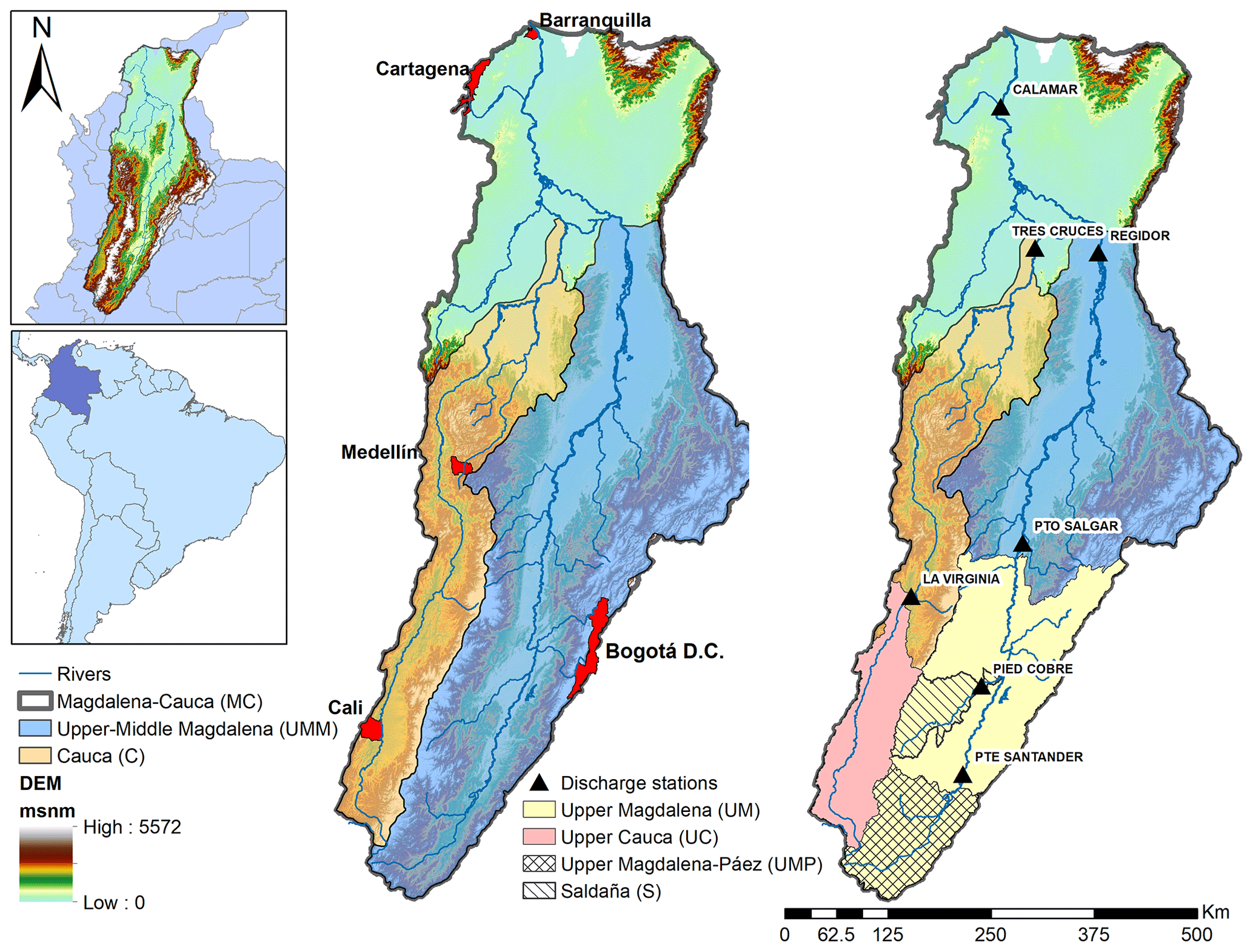
Figure 1Location of the MC Basin in Colombia, as well as the sub-basins considered in this study. The triangles represent the locations of gauge stations measuring streamflow at the outlets of each (sub) basin.
2.1 Study area
The MC basin is the primary river basin system in Colombia. It occupies a major portion of the country in the tropical Andes, draining an area of ∼276 000 km2, which is about 25 % of the total territory of Colombia (Fig. 1). It has its headwaters high up in the Colombian Andes at an elevation of about 3700 m above sea level and runs for some 1612 km before flowing into the Western Caribbean, in the Atlantic Ocean (López-López et al., 2018; Restrepo and Kjerfve, 2000). The main tributary of the Magdalena River is the Cauca River, which flows along the western part of the basin and joins the main Magdalena River in a wetland area called La Mojana, which is found in the Mompós Depression region. The mean annual river discharge at the gauge station closest to the mouth (Calamar) is approximately 7200 m3 s−1 with mean maximum discharges occurring in November (10 200 m3 s−1), and minimum average flows in March (4050 m3 s−1) (Camacho et al., 2008).
Due to the seasonal migration of the Intertropical Convergence Zone (ITCZ) around the Equator, the climate in the basin is on average bimodal, characterised by two wet periods (March–May and September–November) interspersed with two dry periods. However, this is a basin with high variability, and we can observe that the lower MC basin tends to have a more unimodal behaviour (Urrea et al., 2019), with a continuous wet period from May to November (Fig. S1 in the Supplement). The average annual precipitation in the basin is around 2150 mm, while the annual average potential evapotranspiration is estimated at 1630 mm. The hydroclimatology of the basin is profoundly influenced by the ENSO phenomenon (Poveda and Mesa, 1996). Widespread flood events caused by the La Niña event of 2010–2011 affected some 4 million Colombians and caused economic losses estimated at USD 7.8 billion (Hoyos et al., 2013; Vargas et al., 2018), while the severe droughts caused by the El Niño event of 2015–2016 had quite severe consequences, including water shortages in more than 25 % of the towns, the highest temperatures on record, and numerous fires that impacted several regions in the country (Hoyos et al., 2017).
To analyse the effect of basin size on model performance and GRACE data, we subdivide the macro-basin into several sub-basins (Fig. 1). While the overall basin at Calamar station has an area of ∼276 000 km2, the Upper-Middle Magdalena (UMM) has an area of ∼140 754 km2; the Cauca (C) ∼60 657 km2; the Upper Magdalena (UM) ∼56 992,km2; and the Upper Cauca (UC) ∼17 930 km2. The smaller Upper Magdalena–Páez basin (UMP) has an area of ∼14 450 km2 and the Saldaña basin (S) ∼6645 km2.
2.1.1 GRACE data
The TWS anomalies from GRACE satellites are processed by three centres: the Center for Space Research (CSR) at the University of Texas, the Jet Propulsion Laboratory (JPL) in California, and GeoforschungsZentrum (GFZ, Research Centre for Geosciences) in Potsdam, using two different schemes, spherical harmonic (SH) and mass concentration (mascon) solutions. The similarities and differences between the SH and mascon data are well explained by Scanlon et al. (2016) and Shamsudduha et al. (2017). Bolaños et al. (2020) evaluate the different products of GRACE for the MC basin through the comparison with water balances based on observed data. They conclude that the best representation of TWS in the MC basin is the GRACE TWS product derived from JPL mascon. In this analysis we use the TWS anomalies data available from April 2002 to December 2014 from GRACE RL05 level-3 land JPL mascon solution gridded at 0.5∘ (∼55 km), based on an alternative processing approach which involves parameterising the gravity field with regional mascon functions. This product has only recently become operational (Save et al., 2016; Watkins et al., 2015; Wiese et al., 2016).
All reported data are anomalies relative to the 2004–2009 time-averaged baseline as presented in the original GRACE data. For consistency, all other data series used in this study are calculated as anomalies over their average values for the same period. The missing data due to battery management in GRACE were directly remedied by linear interpolation (Ouma et al., 2015; Xiao et al., 2015; Liesch and Ohmer, 2016; Shamsudduha et al., 2012). Variations in water mass or storage are expressed as an equivalent water thickness (EWT; cm water). The JPL mascon data were retrieved from the Tellus website https://grace.jpl.nasa.gov/data/get-data/jpl_global_mascons/ (last access: 11 February 2019).
2.2 Earth2Observe (E2O) global water resources reanalysis (WRR) data
In the analysis, input data were provided by the E2O project, which takes advantage of various global reanalyses and derived datasets to develop a global WRR (Arduini et al., 2017; Dutra et al., 2015, 2017; Schellekens et al., 2017). This dataset includes the outputs of 10 different GHMs and LSMs, which are available at two resolutions and time ranges, denoted as WRR1 and WRR2. In WRR1, models were forced by the WATer and global CHange (WATCH) Forcing Data applied to the ERA Interim data (WFDEI) meteorological reanalysis dataset (Weedon et al., 2014) at a resolution of 0.5∘ (∼55 km at the Equator) from 1979 to 2012. The WRR2 model runs were forced by the Multi-Source Weighted Ensemble Precipitation (MSWEP) dataset (Beck et al., 2017b) at a resolution of 0.25∘ (∼27 km at the Equator) from 1980 to 2014. Selected models in WRR1 and WRR2 have been calibrated against streamflow data, including LISLFOOD, WaterGAP, HBV-SIMREG and SWBM (Beck et al., 2017a). Model algorithms were also improved between WRR1 and WRR2, i.e. by a better representation of hydrological processes, incorporation of anthropogenic influence, and by integrating Earth observation data (Gründemann et al., 2018). Arduini et al. (2017), Dutra et al. (2015), Dutra et al. (2017), and Schellekens et al. (2017) provide a detailed description of the two datasets and the model improvements. Table 1 provides an overview of models considered in this study, as well as the main changes in the models between WRR1 and WRR2 for those models that have been run using both forcing datasets and at both resolutions. The performance of several of these models has been compared over the MC basin, finding that key water resources management indicators derived using these models compare well against those derived using in situ data (Rodríguez et al., 2019).
In order to compare the different models and the WRR with TWS obtained from GRACE JPL mascon, data for the period from 2002 to 2012 were used in this study as a common period for WRR1 and GRACE, and 2002 to 2014 for WRR2 and GRACE. Data were downloaded from the E2O Water Cycle Integrator portal for the required period and for the required spatial domain (https://wci.earth2observe.eu/, last access: 20 November 2018).
(Lindström et al., 1997)(Beck et al., 2016)(Van Der Knijff et al., 2010)(Van Beek et al., 2011)(Orth and Seneviratne, 2013)(Van Dijk et al., 2014)(Flörke et al., 2013)(Balsamo et al., 2009)(Best et al., 2011)(Clark et al., 2011)(Krinner et al., 2005)(Decharme et al., 2010)Table 1Overview of models and main changes from WRR1 to WRR2. Note that not all models included in WRR1 were run for WRR2, in which case no changes are noted in the table. Models that have been calibrated against publicly available streamflow data are indicated.
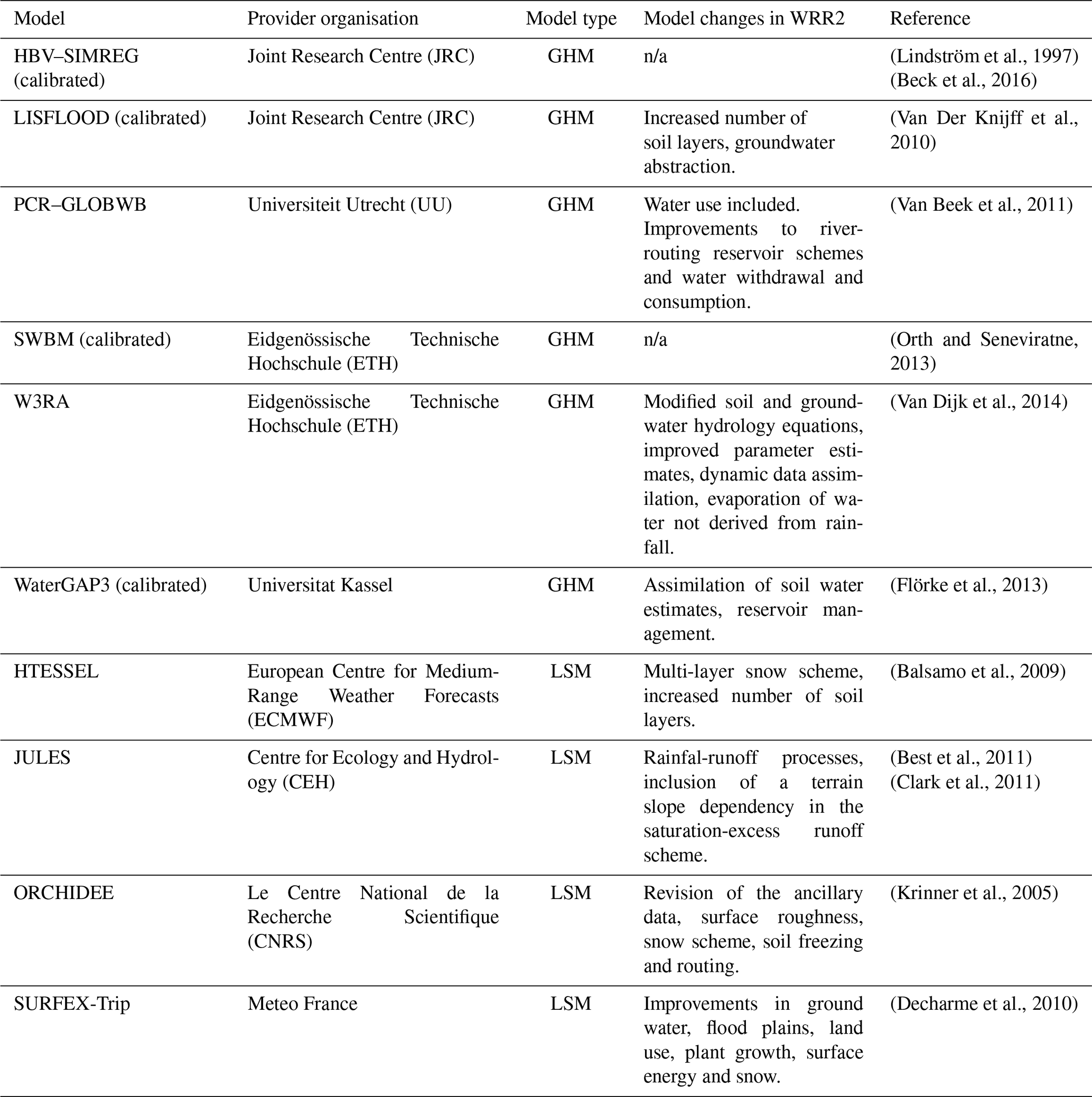
Source: (Schellekens et al., 2017; Dutra et al., 2017).
n/a: not applicable.
2.3 Assessment of model performance
Monthly changes in TWS can be calculated as the result of water balance estimates as presented in Eq. (1), where S is the terrestrial water storage, P and E are the basin-wide totals of precipitation and actual evapotranspiration, and R represents total basin outflow, or the net surface and groundwater outflow. Changes in TWS can also be computed as the sum of the monthly changes in component storages, presented in Eq. (2), where ΔGWS is the change in groundwater storage, ΔSMS is the change in soil moisture storage, and ΔSWS is the change in surface water storage. The ΔCWS is the change in canopy water storage and ΔSWE represents the change in snow water equivalent, which is not considered in this study because the area under snow influence represents less than 0.1 % of the total area of the basin.
Not all of the models contained in the E2O dataset explicitly represent groundwater storage (GWS). For those models that explicitly represent GWS as well as surface and soil moisture components, we apply both equations for evaluating simulated TWS. For models that include only surface water and soil moisture components, we cannot apply the second equation (Eq. 2), which allows a more representative evaluation of TWS since GWS is the largest water component of TWS on land.
For TWS calculated both from models and JPL GRACE data, the values of all cells were averaged for each corresponding monthly time step and (sub) basin extent to construct a time series for each data source and each (sub) basin. This does limit sensitivity to extreme values and the averaging of biases.
Table 2 shows the variables for each model available in the E2O Water Cycle Integrator portal. The table also details if Eq. (1) or Eq. (2) is used to derive simulated TWS changes for each of the two available model resolutions. The symbols in the last four columns identify the datasets and equations considered given their availability, and are used throughout the paper. Also, in all further figures, the blue colour is used to represent GHMs in WRR1, the green colour is used for GHMs in WRR2, the red colour represents LSMs in WRR1, and the yellow colour is for LSMs in WRR2.
Table 2Components used in the TWS change estimation for each model. The last four columns include the symbols and legends used to identify the model resolution and equation used to derive simulated TWS changes. These are used throughout the paper.

* (Schellekens et al., 2017)
In order to understand the variation between TWS changes from GRACE JPL mascon and simulated TWS from models at the basin scale, both model and GRACE time series were disaggregated using the Seasonal-Trend decomposition using Loess (STL) proposed by Cleveland et al. (1990) to estimate the relative magnitudes of water storage variance of different time series components (Eq. 3):
The hydrological performance of the monthly simulated TWS changes from all models was assessed using commonly used model evaluation statistics. We consider Pearson's correlation coefficient (r), root mean square error (RMSE), ratio of RMSE to the standard deviation of the observations (RSR), and the Kling–Gupta efficiency (KGE; Gupta et al., 2009). Pearson's correlation coefficient (r) provides an indication of the linear relationship between the simulated TWS and the benchmark TWS derived from GRACE. The RMSE indicates how close model-predicted values are to observed data, estimating the square root of the variance of the residuals. Lower values of RMSE indicate a better fit. The RSR standardises RMSE using the standard deviation of the observations, and is calculated as the ratio of the RMSE and standard deviation of the observed data. The RSR varies from the optimal value of 0, which indicates zero RMSE or residual variation, and therefore perfect model simulation to an infinitely large positive value. The lower the RSR, the lower the RMSE, and the better model performance (Moriasi et al., 2007). Finally, the KGE index facilitates analysis of the relative importance of different components in the context of hydrological modelling. In the computation of this index, there are three main components involved: the Pearson's correlation, the ratio between the standard deviation of the simulated values and the standard deviation of the observed ones, and the ratio between the mean of the simulated values and the mean of the observed ones. The KGE ranges between −∞ and 1, where 1 indicates a perfect representation of TWS.
3.1 TWS evaluation for the whole MC basin
In order to evaluate the success with which the models represent TWS for the whole basin, we apply Eq. (3) to analyse the monthly time series, seasonality, and long-term trends of TWS for each of the model datasets against the GRACE data. Results are shown in the Taylor diagrams in Fig. 2, which provide a 2D graphical representation of three statistics to indicate how well the simulated pattern matches that of the observations. Similarity is quantified in terms of the correlation(s), the ratio(s) of the normalised RMSE differences between simulated and observed, and the amplitude of their variations represented by the ratio of the standard deviations of simulated and observed (Taylor, 2001). Best performances are for values of a correlation close to 1, with a low RMSE, and a ratio of standard deviations close to 1. Figure 2 shows Taylor diagrams for the complete monthly time series (a), the seasonality (b), and the long-term trends (c). In all cases the corresponding constituents of the GRACE JPL mascon dataset are used as reference. In this figure, as in all further figures, a blue colour is used to represent the GHMs in WRR1 and a green colour is used for the GHMs in WRR2. The LSMs in WRR1 are represented with a red colour, while LSMs in WRR2 are shown in yellow (see also Table 2). Model runs derived from WRR1 are denoted as “R1” for brevity, while those derived from WRR2 are denoted as “R2”, as well as models denoted “Eq1” or “Eq2” refer to the Equation used to estimate TWS.
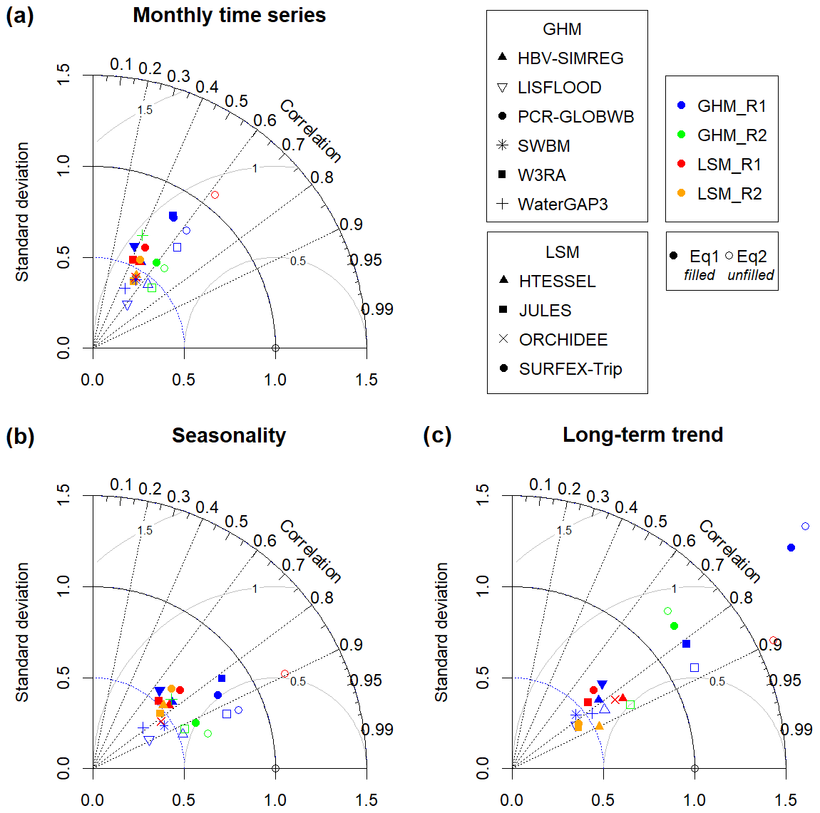
Figure 2Taylor diagrams between each model output and GRACE data for the Magdalena river basin for (a) monthly time series, (b) seasonality, and (c) long-term trends. Models from the first reanalysis WRR1 are denoted as R1, and R2 denotes the second reanalysis WRR2.
From Fig. 2 it is not possible to clearly distinguish which of the models in the total 23 datasets from GHM WRR1, GHM WRR2, LSM WRR1, and LSM WRR2 better represents TWS when compared to GRACE. It is noteworthy that correlations are better for almost all models when considering seasonality and long-term trends. For the monthly series, the correlations of the models range between 0.36 and 0.68, with the highest correlation corresponding to the W3RA R2Eq2 and the lowest to LISFLOOD R1Eq1. However, for almost all models (except Surfex-Trip R1Eq2) smaller standard deviations are found than those observed by GRACE. For the representation of seasonality, we observe that correlations increase in all models, with the highest correlation found for PCR-GLOBWB R2Eq2 (r=0.96) and the lowest for LISFLOOD R1Eq1 model (r=0.65). We also observe that GHMs are the models with good correlation and whose standard deviations are closer to those observed, particularly PCR-GLOBWB R1Eq1, PCR-GLOBWB R1Eq2, W3ERA R1Eq1, and W3RA R1Eq2 models. For long-term trends, an increase in correlations is also observed. The highest correlation is now found for the HTESSEL R2Eq1 model (r=0.91) and the lowest for WaterGAP3 R2Eq1 (r=0.23). Standard deviations for most models are lower than those observed, indicating a variability that is too low. The WaterGAP3 R2Eq1, PCR-GLOBWB R1Eq1 and Eq2, and SurfexTrip R1Eq2 models differ in that these show very high standard deviations compared to those observed in GRACE TWS.
We additionally analyse the residuals in Eq. (3), finding that these residuals are normally distributed at the 95 % confidence level and are poorly auto-correlated. We therefore consider these residuals as noise, with the greater part of the variability of the time series that we observe explained by the seasonality and long-term variability (see Figs. S4 and S5 in the Supplement).
3.2 TWS monthly values evaluation
To provide an overview of the range in performance metrics comparing TWS at the sub-basin scale to GRACE-derived TWS, Fig. 3 groups the correlation, RMSE, and RSR by model type (GHM and LSM) and reanalysis (WRR1 and WRR2). We observe an improvement in the performance of the WRR2 models over the WRR1 models, with an increase in correlation values and decrease for both RMSE and RSR.
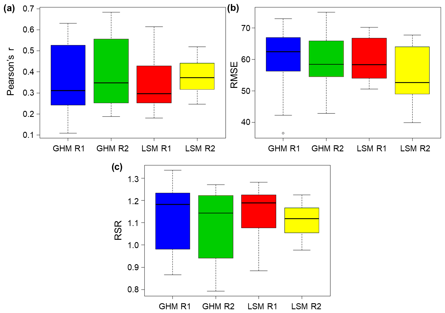
Figure 3Distribution of model performance for the three metrics considered, grouped by model type (GHM or LSM) and forcing/resolution (WRR1 and WRR2). Three performance metrics are shown: (a) Pearson’s r, (b) RMSE, and (c) RSR.
This is further explored in Fig. 4, showing the relationship between TWS of the sub-basin area within the MC basin and the error statistics for the models in WRR1 and WRR2. To allow comparison, error statistics are normalised and standardised. These results clearly demonstrate the detriment in model performance as basin size decreases. This is best observed in the KGE statistic (Fig. 4a). It is evident that the models are generally able to better capture the hydrology for the main basins in both WRR1 and WRR2. For the UM sub-basin (56 992 km2) and the smaller sub-basins, there is a marked decrease in performance, although the only slightly larger C basin (60 657 km2) shows much better performance. This provides an indication of the basin size at which the models are capable of capturing TWS. It also illustrates the difference in forcing, resolution, and the model’s improvements made in WRR2 over WRR1. For WRR1, the best performance for the MC and UM basins is found with the HBV-SIMREG R1Eq2 model; the W3RA R1Eq2 model performs reasonably well for the UMM and C basins; and the SWBMExp1 R1Eq1 model has the best performance for UC, UMP and S basins. All three of these models are GHMs. For WRR2, the best performance in almost all basins is found with the W3RA R2Eq2 model, though for the smaller basins (UMP and S) it is found to be the JULES R2Eq1 model. The first of these is a GHM and the second an LSM. The models with the lowest KGE values are LISFLOOD R1Eq1 for MC, UMM, and UM basins, WaterGAP3 R2Eq1 for C, and PCR-GLOBWB R1Eq2 for the last three basins. For models that have been run for both WRR1 and WRR2, it is not consistently found that the WRR2 runs have improved performance for all basins. For instance, PCR-GLOBWB WRR1 is better than WRR2 for only the C basin, while HTESSEL WRR1 is better than WRR2 for the C and UC basins. Furthermore, WaterGAP3 presents better performance for WRR1 in all basins, while Surfex-Trip has the highest values for WRR1 than for WRR2 for all basins, except for the two smaller basins. For W3RA, the best performance is consistently found for WRR2 across all basins.
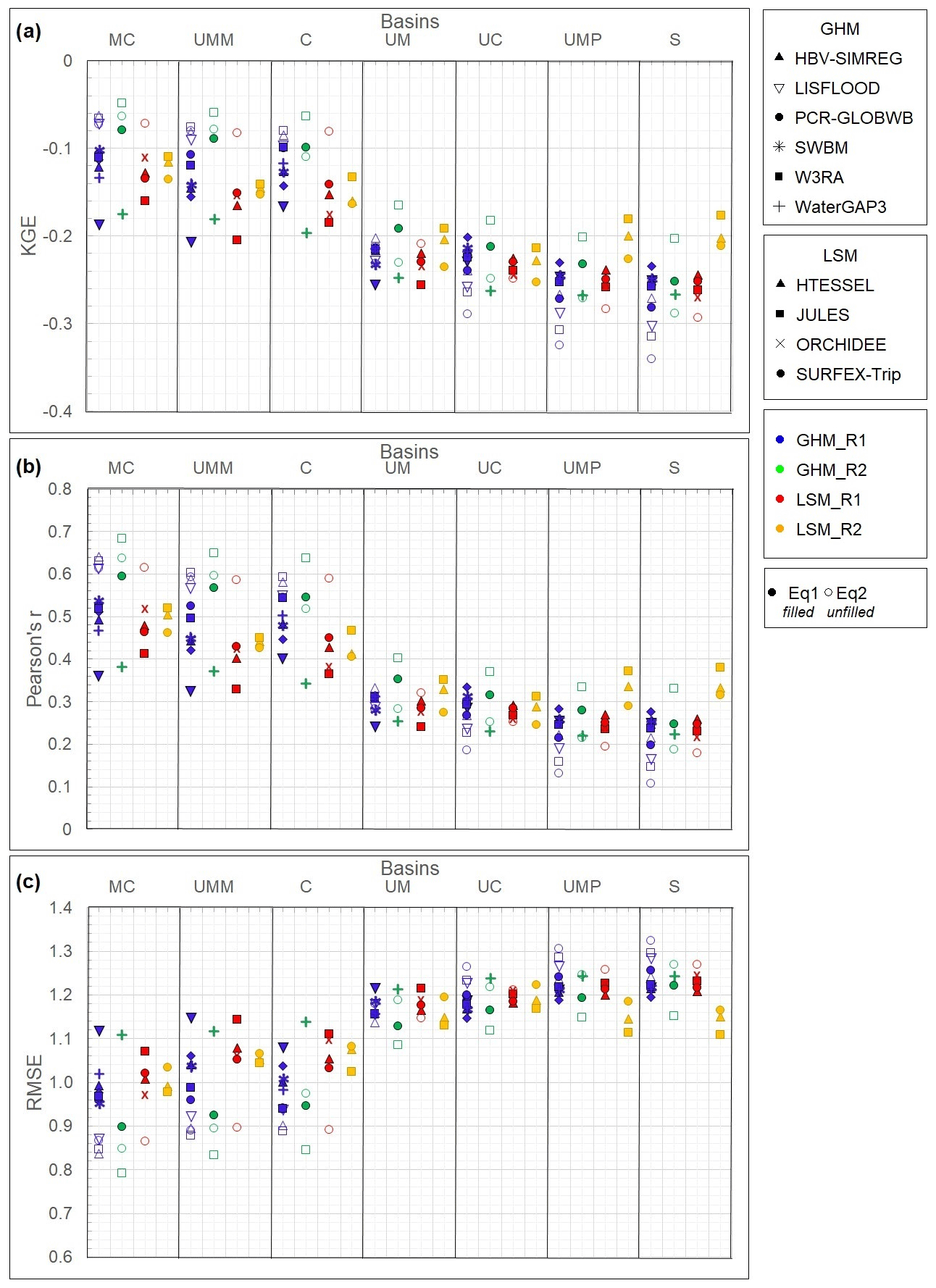
Figure 4Performance statistics between GRACE and the GHM (blue and green points for WRR1 and WRR2, respectively) and LSM (red and yellow points for WRR1 and WRR2, respectively) at different scales in (a) the KGE index, (b) Pearson’s r, and (c) the RMSE. The basins are ordered by size (largest to the left), and the data are standardised and normalised.
In Fig. 4b we display the Pearson’s correlation coefficient r for each model. For both WRR1 and WRR2, the best performances are consistent with the KGE index. With some exceptions, the WRR2 models show improved performance over WRR1. The model with the highest correlation in all basins is W3RA R2Eq2. Models with the lowest RMSE alternate between W3RA R2Eq2, WaterGAP3 R1Eq1, and JULES R2Eq1. The opposite case is WaterGAP3, and SURFEX-Trip only has an improvement in WRR2 over WRR1 within the UMP and S basins. The RMSE in Fig. 4c shows consistency with the other statistics. The lowest values again correspond to W3RA R2Eq2 and JULES R2Eq1 showing the best performance.
Even though some models perform relatively well, the overall performance of the models is generally poor. Average KGE remains negative for all models and sub-basins, and the average Pearson’s r value does not exceed 0.5 in most cases. We highlight the decrease in the performance of all models for the smaller basins. The shift between the C and UM basins, with areas of ∼60 657 and ∼56 992 km2, respectively, is interesting, and although the specific catchment conditions in these two basins may lead to an apparent step change, the reduction of performance of the models for the smaller basins is clear. It is worth noting that GRACE resolution will start having more limitations in these smaller basins.
The spatial relationship between TWS monthly values of GRACE, models with both reanalysis WRR1 and WRR2, and the models with only WRR1, respectively, are presented in the supplementary material (Figs. S2 and S3). In these figures we rescale the GRACE TWS and the models from 0.5 to 0.25∘ using bilinear interpolation to interpolate from one rectilinear grid to another, to be consistent with the finest resolution WRR2 models. The model with the highest correlation values is W3RA Eq2 WRR2. The maximum values presented in the maps are close to 0.8 and are located mainly towards the north of the macro-basin, with the minimum values towards the south. This is coherent with Fig. 4, in which we observe a reduction in performance of all models upstream of the UM basin. This suggests that not only basin size is relevant to the performance of each model. The prevailing pattern could suggest that it is related to hydrological process, or more likely to the presence of storages in these areas that the models are not simulating properly. In Fig. S2 it is also clear that there is an improvement in the spatial correlations of models when forced with WRR2 rather than WRR1, except for WaterGAP3.
3.3 TWS seasonality and evaluation of long-term trends
To assess the seasonal signals and long-term trends of the models against GRACE TWS, we show the Pearson’s r coefficient and RMSE statistic for all sub-basins in Fig. 5. We observe a similar pattern as displayed in the Taylor diagrams presented in Fig. 2 for the macro-basin, but now highlighting model performance with decreasing basin size. We observe the same shift in the performance of models for basins with the size of the UM basin and smaller for both seasonality (Fig. 5a, b) and long-term trend (Fig. 5c, d). The Pearson’s r values for both is better than in the analysis of monthly values (Fig. 5a, c). For seasonality, the highest r coefficient is found in PCR-GLOBWB R2Eq2 for the MC and UMM basins, and in W3RA R2Eq2 for the remaining sub-basins, which coincides with the lowest RMSE in Fig. 5b. For long-term trends, the highest r coefficient is presented in HTESSEL R2Eq1 for MC, in JULES R2Eq1 for UMP, and in W3RA R2Eq2 for the remaining sub-basins, which coincides with the lowest RMSE in Fig. 5d. The WaterGAP3 R2Eq1 presents the lowest performance for all sub-basins in the long-term trends.
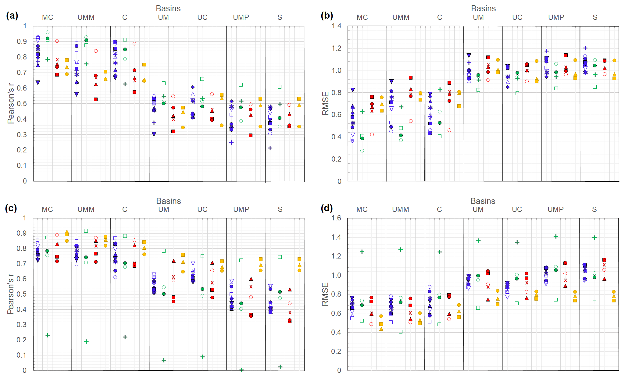
Figure 5Performance statistics for the seasonality (a–b) and long-term trends (c–d) of GRACE and the GHMs (blue and green points for WRR1 and WRR2, respectively) and LSMs (red and yellow points for WRR1 and WRR2, respectively) at different scales in (a, c) the Pearson’s r coefficient and in (b, d) the RMSE.
The seasonality found for the GRACE data, as well as for each group of models and each sub-basin, is presented in Fig. 6. In general, we observe good agreement between TWS from the models and GRACE for the main basins. The bimodal behaviour in all models and GRACE data is consistently represented as a consequence of the dominant bimodality of precipitation in the whole MC basin (Poveda, 2004). However, for the UM basin and smaller basins, the models tend to overestimate the second peak during the SON (September–October–November) season. The maximum peak in GRACE for all sub-basins occurs in the month of May, while in the models it varies.
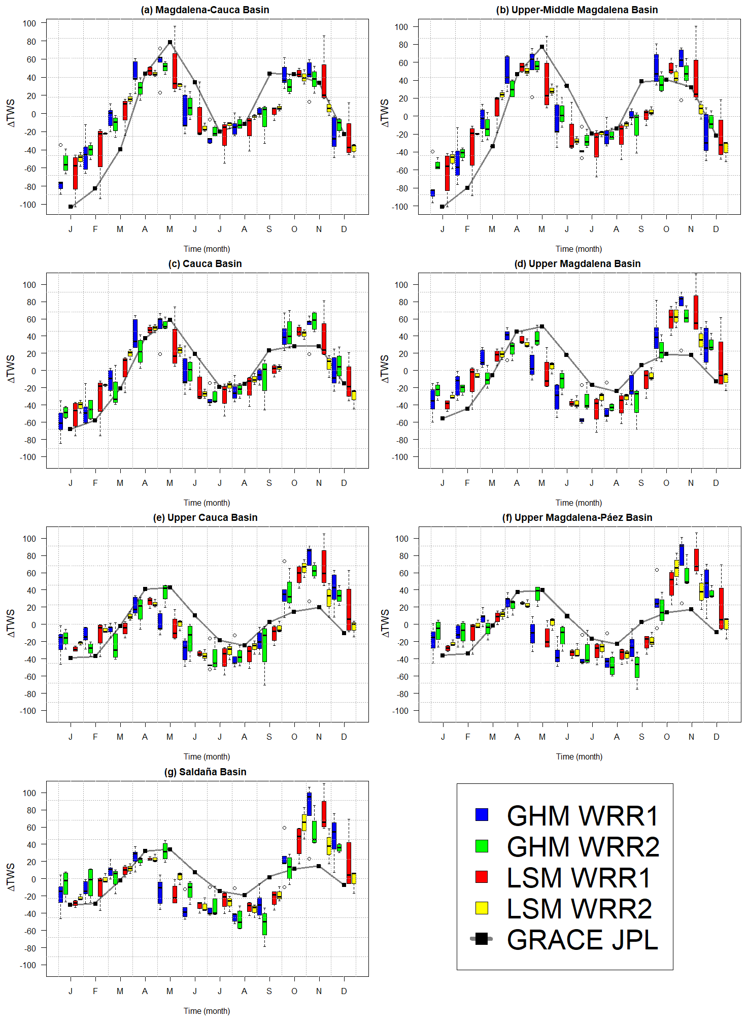
Figure 6Comparative boxplots between the climatology of GHMs and LSMs, and GRACE JPL for each sub-basin.
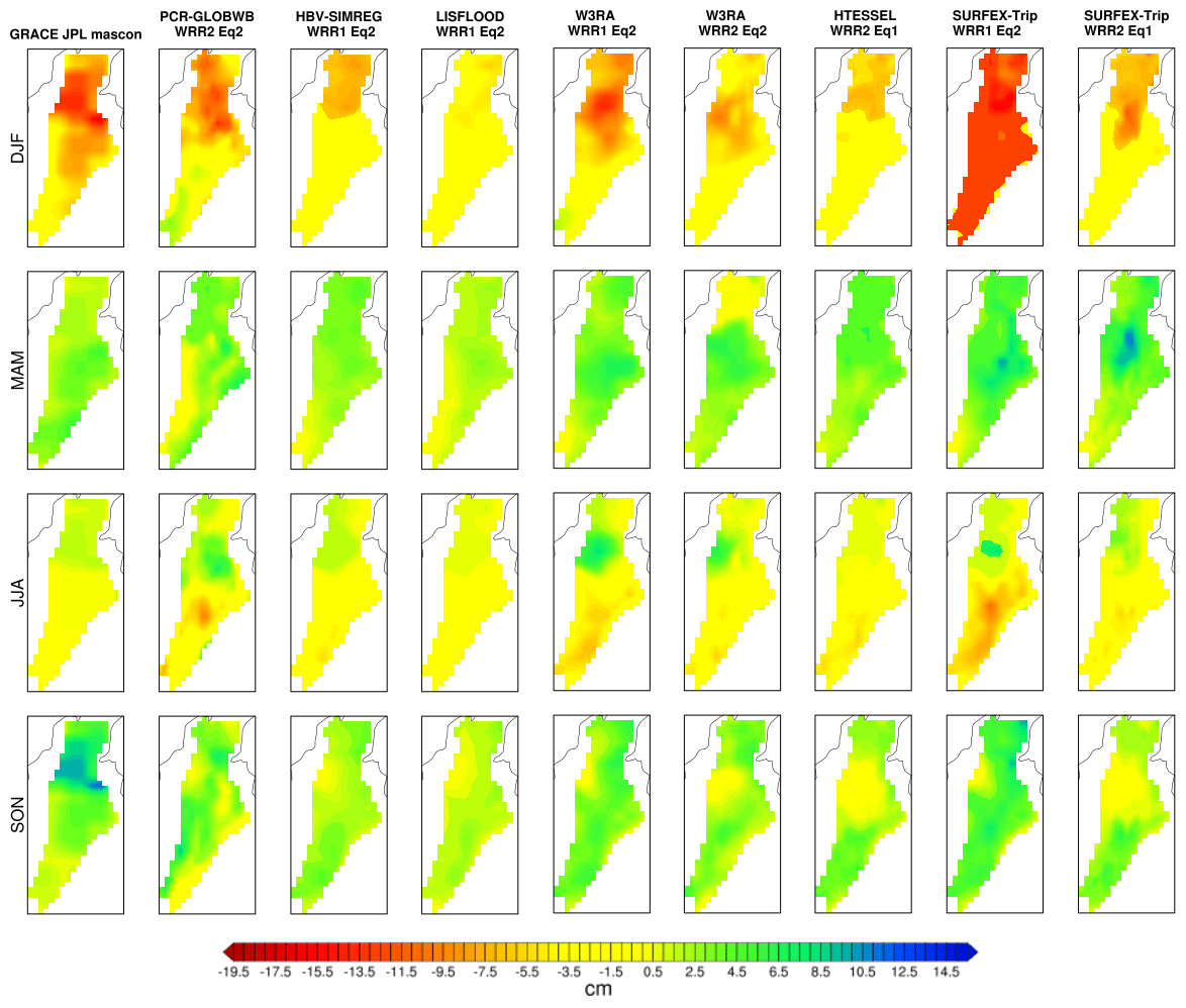
Figure 7 compares the seasonal maps of TWS estimated for GRACE, the models with the highest correlations (see Figs. S2 and S3), and models that perform similarly. The seasonal maps of TWS for the other models are shown in the supplementary material (Figs. S6 and S7). Here, we observe that the amplitudes for most models are smaller than for the GRACE data. This implies that the models tend to underestimate seasonal variation. For DJF (dry season), the models tend to be consistent with GRACE, with the lowest biases found in the north. In general, for the basins, the values of TWS are negative or near zero. On the other hand, MAM (the first wet season) shows the opposite case with positive values throughout the macro-basin, with some exceptions towards the north (W3RA R2Eq2). In JJA (dry period), we again observe consistency. There is a transition between the two rain periods, with positive bias in the north and negative bias in the south of the basin. In SON the models differ spatially with GRACE. The highest values of TWS from GRACE are found in the north of the basin in SON. This part of the basin is dominated by the La Mojana wetlands. In contrast, the models mostly present biases in the area of La Mojana close to 0 and higher TWS values towards the south of the basin. These higher values in the south correspond with the peaks observed in Fig. 6. This behaviour is likely due to the poor representation of the wetlands in the models. The buffering capacity in the models is poorly represented, which means that these dry out too much in the drier DJF period and cannot represent the increased storage in the wet period during SON in the La Mojana area, which can be observed by GRACE. For the second dry season, the fact that the climate becomes more unimodal to the north (see Fig. S1) may also contribute. Both drying and wetting may also be overestimated by the models as observed in the south, especially, during JJA and SON, and SURFEX-Trip R1Eq2 during DJF.
Finally, we explore the agreement between the models and GRACE for the long-term component. Figure 8 shows the time series for GRACE JPL (black line) as well as for each model group: GHM WRR1, GHM WRR2, LSM WRR1, and LSM WRR2 (blue, green, red, and yellow lines, respectively). We present the graphs for MC, C, UM, and S basins, as the other sub-basins are similar to these and are shown in the supplementary material (Fig. S8). The MC and S basins are the largest and smallest basins, respectively, while the change in model performance occurs between the C and UM basins. Large discrepancies between models and GRACE can be seen, with these increasing as basin size decreases. We observe that WaterGAP3 R2Eq1, PCR-GLOBWB R1Eq1 and Eq2, and SURFEX-Trip R1Eq2 (the first two are GHMs and the last one is LSM) overestimate both high and low peaks. In contrast, LISFLOOD R1Eq1 and SWBM R1Eq1 outputs are relatively flat, underestimating both the high and low peaks. However, all models are able to capture the increase in TWS during the 2010–2011 ENSO event (La Niña), likely due to the (common) precipitation forcing. Better performance is shown for the LSMs than for GHMs in general, although the results for W3RA R2Eq2 are closest to observations.
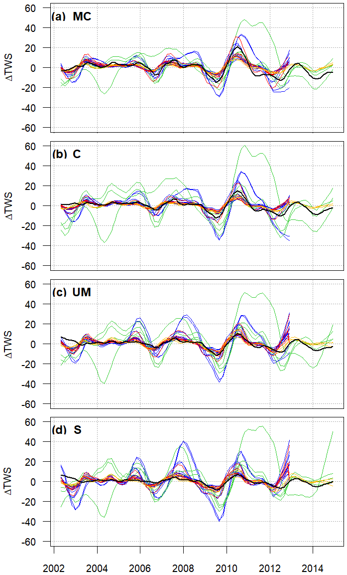
Figure 8Long-term trends of time series for the models and GRACE for (a) MC, (b) C, (c) UM, and (d) S basins. The black lines indicate the GRACE JPL, the blue and green lines represent the GHM WRR1 and WRR2, respectively, the red lines represent the LSM WRR1, and the yellow lines show the LSM WRR2.
4.1 Evaluation of the performance of the models
To summarise the performance results of the models with respect to GRACE, we present the performance metrics for each model and WRR in Fig. 9. Higher score values (blue boxes) correspond to a better performance in representing TWS, while lower score values (red boxes) indicate a poor representation for monthly time series, seasonality, and long-term trends. This shows that the WRR2 models tend to exhibit better performance than the lower-resolution WRR1 models. This is coherent with the results of Gründemann et al. (2018), who assessed simulated discharges from 7 of the 10 models studied here, as well as the ensemble mean of those models, focusing on the occurrence of floods in the Limpopo River basin in southern Africa. The exception of this improved performance is found for WaterGAP3, which shows much poorer performance for WRR2, particularly in the representation of long-term trends.
Since the models have the same input/forcing for each WRR, differences in simulation results can only be attributed to the model structure and internal model dynamics. A number of factors could contribute to the notably poor performance of WaterGAP3 in WRR2 for the study area. These include modifications made to the simulation of hydrological processes, the way in which reservoir management is represented, and its calibration. However, Dutra et al. (2017) note that the modifications made to WRR2 primarily affect the water stored in the reservoirs and not the surface runoff, evapotranspiration, or other surface fluxes. While there are a large number of reservoirs in the basin, these are primarily used for hydropower generation and, to a lesser extent, to serve irrigation, flood control, or other purposes. As a result, the degree of regulation of these reservoirs is found to be quite low (Angarita et al., 2018). The reservoir release scheme in the WaterGAP model follows a more generic concept, independent of the primary purpose of the reservoir (Müller Schmied et al., 2021), and thus may misrepresent the dynamics of the reservoir storage in this basin. The WaterGAP3 model was also found to perform poorly with respect to other GHMs in a snowmelt-driven catchment in northern Canada. The latter also includes extensive regulation for hydropower production (Casson et al., 2018). In contrast, however, for the Limpopo River basin in southern Africa, the WaterGAP3 model in WRR2 demonstrated the best performance in simulating flood events among the same models considered here (Gründemann et al., 2018). This is also an extensively regulated basin, though reservoirs in the Limpopo River basin primarily serve irrigation and flood control, the operation of which may be better captured by the generic reservoir operation rules. This underlines the challenge of simulating reservoirs and their sector-specific operation in (global) hydrological models (Rougé et al., 2021). Beck et al. (2017a) show that WaterGAP performs well in reproducing streamflow, but also suggest that the WaterGap baseflow index is not good. This could point to an unbalance between internal hydrological processes, which may have been induced by the calibration. Similarly, for LISFLOOD R1Eq1 we observe relatively poor performance in reproducing TWS anomalies. In contrast, the same model, but using different equations (LISFLOOD R1Eq2), performs better, which suggests that although the precipitation forcing is common, the calibration against streamflow would primarily affect the fluxes of evapotranspiration and runoff. Another reason could be that LISFLOOD is reported to underestimate quick-flow response (see Beck et al., 2017a), which could lead to less-pronounced seasonality than the other models (as shown in Fig. 5). The calibration of models against observed discharges may improve model results at basin outlets, but may be detrimental to the representation of internal states and fluxes. This may be particularly true where there are biases in the forcing data due to the complex topography of the basin.
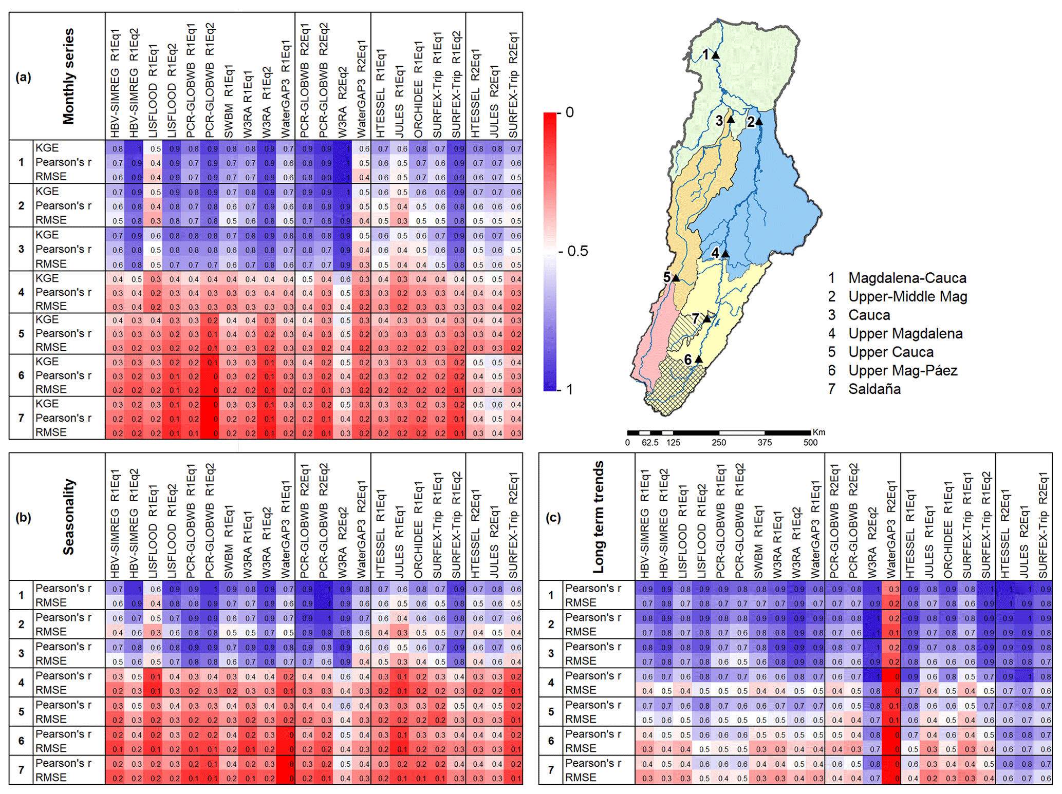
Figure 9Summary figure of the performance among models with respect to GRACE data. Statistics of KGE, Pearson’s r, and RMSE were rescaled between 0 and 1, with 0 being the worst performance among the models and 1 being the best performance. The evaluation is presented for (a) the monthly time series, (b) the seasonality, and (c) the long-term trends.
Figure 9 shows that over the MC basin as a whole, the TWS change computed from W3RA WRR2 using Eq2 best represents the signal of the GRACE data; including the monthly time series, seasonality, and long-term trends. The performance metrics do demonstrate, however, that for the different sub-basins, the best performing models include both GHMs and LSMs. Although the W3RA model is among the best performing models in all basins, for the monthly time series, JULES R2Eq1 performs best in the smaller basins. Besides W3RA, the seasonality is captured equally well by PCR-GLOBWB R2Eq2, while for long-term trends, HTESSEL R2Eq1 and JULES R2Eq1 (both LSMs) also show good agreement to the GRACE data. Each of these models performed well with similar statistics throughout the basin, despite their differences in structure.
Zhang et al. (2017) evaluate the TWS estimates from 4 hydrological models (2 GHMs and 2 LSMs) and GRACE in 31 of the world's largest river basins. Although the MC basin is not included in their study, they similarly find that the performance of the models varies from basin to basin, even within the same climate zone. They conclude that the variation in performance could be due to model structure, parameterisation, the different water storage components included in the calculation of TWS, as well as being connected to the differences in runoff simulation and evaporation schemes (Zhang et al., 2017; Ramillien et al., 2006). In our case, the best performing models (W3RA, HTESSEL, and JULES) calculate evapotranspiration using the Penman–Monteith method, and saturation- and infiltration-excess for calculating runoff. However, the worst performing models (LISFLOOD and SURFEX-Trip) use these same schemes, while WaterGAP3 uses the Priestley–Taylor method for evapotranspiration and beta function for runoff. The routing scheme, whether human water use is incorporated, and time step can also cause significant differences between the models. Within the ensemble of models considered here, there are, however, multiple differences between models structures, making it difficult to uniquely identify model structures that singularly contribute to improved performance. This would imply that the relationship between model performance and model structures that best represents the processes in a tropical basin such as the MC is as yet inconclusive.
However, Schellekens et al. (2017) note that the W3RA model applies a Gash event-based model to simulate interception, an important hydrological process in tropical basins (Miralles et al., 2010), and this could contribute to its relatively good performance. Most models tested here follow a single reservoir and potential evaporation process to compute interception, while other models do not include an interception scheme. Additionally, models that include a groundwater component, and for which the performance can be evaluated using Eq. (2), show better performance over the same models when using Eq. (1) to compute TWS (Fig. 9). Nevertheless, further analysis is required in which the representation of internal processes, evapotranspiration, and runoff approaches is evaluated in depth. Moreover, it is important to note that the ranking of model performance may be quite different in different basins, and also depends on the aim of the research. However, we underline the importance of using a fundamental variable such as TWS as a proxy to inquire internal model states to benchmark model performance.
4.2 Performance in representing seasonality and long-term trends
The differences between models in representing TWS changes for seasonality and long-term trends may be due to various reasons. Following Scanlon et al. (2019), differences in seasonal amplitudes of TWS between models and GRACE can result from uncertainties in models, in GRACE, or in both. These uncertainties may come from the scheme of modelled storage capacity and storage compartments included in each model (Table 2), uncertainties in modelled inflows/outflows, and uncertainties in modelled human interventions in the case of GHMs, or lack thereof in LSMs. Storage capacity and compartments such SWS and GWS are critical in tropical basins, where the magnitudes of the TWS seasonal amplitudes are high, driven by seasonal precipitation (Scanlon et al., 2019). The average bimodal behaviour is evident in the seasonal signal of TWS from GRACE and models, but the peak during the SON season in the models is greater in the smaller basins. The peak during the SON season logically follows the precipitation used to force the models, but in GRACE this peak is generally lower than the MAM peak. The overestimation (underestimation) of modelled seasonality of TWS changes relative to GRACE in the study area could result from underestimation (overestimation) of the storage capacity. A possible explanation of the differences in the peaks observed during these two wet seasons as observed in GRACE is that the MAM wet season is preceded by a strong dry season. As the soil receives a large amount of water, this infiltrates and recharges groundwater, and thus adds to TWS in the basin; the soil becomes saturated; and the remainder becomes surface runoff. For the second wet season (SON), which is generally stronger and with greater precipitation quantity (Poveda, 2004), the soil is not as dry as in the first wet season, and therefore soil saturates more rapidly, generating more runoff that quickly leave the basins, with smaller changes in TWS (e.g. in groundwater) as consequence.
Due to the poor representation of the storage capacity in the models, these may be overestimating changes of TWS in SON, especially in the south where the topography is more complex. The heterogeneity of climate in the basin may also be important since there is a tendency towards a unimodal climate to the north of the basin with a much less pronounced JJA dry season (Urrea et al., 2019). Pokhrel et al. (2013) establish similar conclusions in the Amazon basin where model representation of the groundwater – vadose zone – surface water dynamics is important in representing seasonal dynamics.
Similarly, discrepancies in long-term trends in TWS may be related to uncertainties in models and/or GRACE. Scanlon et al. (2018) evaluate seven different global models against GRACE. Considering initial conditions, water storage compartments and capacity related to model structure, precipitation uncertainty, and model calibration, they conclude that the models considered underestimate large decadal water storage trends relative to GRACE data. In this study, the models have the same input/forcing for each WRR and the majority of models have not been calibrated, while for those models that have been calibrated (Table 1), the calibration was not specific to the MC basin (Beck et al., 2017a). This implies that differences must largely be due to model structure (e.g. representation of water storage compartments) and parameterisation (e.g. capacity of compartments) (Dutra et al., 2017). The way each model computes the storage capacity could be related to the lack of storage compartments, soil profiles (thickness and number of layers), or exclusion of processes such as river flooding (Scanlon et al., 2018). One of the clear factors is that most LSMs do not model SWS and GWS compartments, with the exception of Surfex-Trip. However, the inclusion of SWS and GWS is not conclusive for a good agreement with GRACE in our study since Surfex-Trip overestimates long-term trends and the LSMs in general have a better performance than most GHMs (Figs. 5c, d and 9c). Models also differ in how storage compartments such as the soil layer are discretised (Schellekens et al., 2017). While W3RA has 3 soil layers and shows good agreement, WaterGAP only has 1, and SurfexTrip has 14 soil layers. More than the number of soil layers, the thickness and total soil depth could be important variables for the calculation of storage capacity. Swenson and Lawrence (2015) report that the thickness of the profile required to replicate GRACE TWS variability is up to 8–10 m in tropical regions (e.g. Amazon, Congo) and in South Africa, while most models considered here have a soil thickness of between 1 and 4 m (Schellekens et al., 2017; Dutra et al., 2017), thus limiting the storage dynamics.
4.3 Basin scale analysis
As basin size reduces, the performance of models is found to decrease. Here it is important to highlight that GRACE measurements and leakage uncertainties increase with decreasing basin size (Scanlon et al., 2016). In Figs. 4 and 5, the shift occurs between C (∼ 60 657 km2) and UM (∼ 56 992 km2). Currently, basins with a size of ∼ 63 000 km2 can be resolved to an error level of 2 cm in terms of equivalent water height (Vishwakarma et al., 2018), which would agree to the size smaller than that which we find for a marked decrease of performance. Nevertheless, when we analyse the spatial correlation maps (Figs. S2 and S3) and the seasonal maps (Fig. 7), we observe that there are large discrepancies for the south of the macro-basin.
The southern part of the basin corresponds to an area with a more complex topography. While the global models generally provide a poor representation of the wetlands in the north of the MC basin, the hydroclimatology of the mountainous areas is more heterogenous as precipitation not only depends on the macroclimatic phenomena such as the ENSO and ITCZ migration, but is also influenced by other atmospheric circulation mechanisms such as mesoscale convective systems, soil–atmosphere interaction processes, and local circulation patterns (Poveda, 2004). Furthermore, the interplay between the Orinoco and Amazon basins plays an important role in the moisture availability and precipitation for the UM sub-basin, which would add complexity to the hydro-climatological characteristics in this region, posing a challenge for models and their calibration (Bedoya-Soto et al., 2019).
Additionally, it is important to highlight the presence of high-altitude montane wetlands (Páramos). These are one of the most important ecosystems in Colombia and provide an important source of water supply for many of the big cities in the Andean region (Rodríguez and Armenteras, 2005). The hydrological processes in these Páramos are poorly understood, making the simulation of the water balance and storage dynamics difficult (Buytaert and Beven, 2011). Moreover, the upper basins are highly intervened by human activities, including several reservoirs, which challenge the models by simulating flows and water storage compartments. Gründemann et al. (2018) point out that models that only capture natural flow conditions, and do not take artificial reservoirs and water usage into account, may be able to reasonably estimate runoff volumes, though they do tend to overestimate the actual magnitude of discharges. Their results suggest that GHMs would have better performance over LSMs, particularly those that include human interventions. While we do observe this to be the case for the general MC as well as selected sub-basins (UMM and C), when comparing monthly time scales of TWS for the smaller basins, we find that the LSM WRR2 have a better agreement over GHMs (Fig. 9).
Figure 9 also shows that the deterioration of model performance for basins smaller than 60 000 km2 is most clearly seen for those models where GRACE TWS is used to benchmark models that represent internal model stocks, such as groundwater, using Eq. (2). Benchmarking those same models using Eq. (1) results in a much more varied picture, which is also seen in the results of Rodríguez et al. (2019), who tested several of the global models used here as well as (calibrated) regional models against observed discharges from 88 gauges across the MC basin. This did not reveal a clear pattern in model performance across the basin.
With the overall poor and decreasing availability of observed hydrological data in tropical basins, there is an increasing interest in the use of remote-sensing data and models to study water resources, as well as the impact of climate change and human influences on water resources. The recently developed eartH2Observe (E2O) global water resources reanalysis (WRR) dataset provides hydrometeorological data of sufficient length and coverage to complement observed data in water resources assessments (WRA). However, insufficient availability and poor spatial distribution of observed data mean that independent evaluation of these reanalysis data in representing key hydrological processes and storage dynamics in these basins is difficult. On the other hand, the GRACE satellite dataset is a recent and powerful tool that provides independent and distributed observations of Total Water Storage (TWS) in river basins, giving insight into the water storage dynamics that would not be possible through conventional observations. These data provide an opportunity to benchmark water storage dynamics of the models used in WRR and explore the question of how well these represent basin TWS dynamics.
We evaluate the representation of TWS changes from 10 models in the E2O dataset, including 6 global hydrological models (GHMs) and 4 land surface models (LSMs). We benchmark the performance of these models in the Magdalena–Cauca basin in Colombia, a medium-sized tropical basin that can be considered unique to tropical basins, given its comparatively well-developed monitoring network. We assess the potential of the two global WRRs (WRR1 and WRR2) available from the E2O dataset by studying the performance of these models in simulating TWS changes through commonly used statistics.
Performance statistics reveal that the variability of GRACE TWS is better captured by the models in the larger basins compared to performance in the smaller, nested, basins. Basin sizes, at which both WRR1 and WRR2 models are able to provide a better representation of the hydrological behaviour, are observed for areas above around 60 000 km2, with significantly poorer performance for smaller catchment sizes. Although this could be attributed to the relatively coarse resolution of the GRACE TWS data used as a benchmark, and consequent uncertainty and signal leakage in smaller basins, we observe that the inadequate ability of the models to capture the hydrological process and storage dynamics in the south of the basin contribute to this poor performance. This part of the basin has a more complex topography and a higher degree of human intervention, such as reservoirs. Additionally, there are high montane wetlands (Páramos) that have an essential role in regulating water resources. Although our benchmark does not reveal specific model structures that contribute to improved performance of either GHMs or LSMs, our results do suggest that the representation of processes such as interception and storage dynamics in the soil column, including groundwater, contributes to better model performance.
In general, models included in the higher-resolution WRR2 dataset have better performance than the models in the lower-resolution WRR1 dataset. This shows that the continued efforts to improve global models, either through improved and higher-resolution forcing or improved and higher-resolution model structures and parameterisations, can enhance the models' ability to reproduce observed TWS and simulate water resources variability. However, poor representation of specific processes such as reservoir operation through a scheme that is too generic, common to global models, may obscure these improvements.
Our comparison highlights the relevance of using independent, remote-sensing data to benchmark large-scale models in specific hydro-climatological settings, including tropical basins. Our results suggest future directions for model development, highlighting the appropriate representation of water stocks and related processes. It is relevant that models that do include explicit representation of the internal storage dynamics allow for a more direct benchmarking of modelled TWS against the TWS data from GRACE. This would improve the assessment of model performance compared to benchmarking models against indirectly calculated TWS variability, as derived from the balance of precipitation, evaporation, and observed basin outflow; thus helping to discriminate models with better structures and process representation.
Although the disparity between GRACE and the models is subject to uncertainties in both, the quality of GRACE data will continue to improve in the foreseeable future. In this study, we use the most recent GRACE release (RL5) before the constellation of satellites that provided these data discontinued their service (Watkins et al., 2015). A GRACE follow-on mission as a successor to the original GRACE mission was launched in May 2018, with data becoming available shortly for future research. These continued advances in GRACE data and their use to independently benchmark internal states of hydrological models will improve our understanding of water resources and reduce uncertainties in using these models in water resources projections under climatic change and increasing human interventions.
Data used in this manuscript are freely available in the following web pages: JPL mascon data were retrieved from the Tellus website https://grace.jpl.nasa.gov/data/get-data/jpl_global_mascons/ (last access: 11 February 2019; Watkins et al., 2015); earth2Observe models data were downloaded from the E2O Water Cycle Integrator portal https://wci.earth2observe.eu/ (last access: 20 November 2018); https://doi.org/10.5281/zenodo.167070 (Schellekens et al., 2016). Additionally, we present the TWS data from GRACE and the estimated values for each model derived from the E2O data for the study area in the Supplement.
The supplement related to this article is available online at: https://doi.org/10.5194/hess-26-4323-2022-supplement.
SBC, MW, JFS, and TBV contributed to the conceptualisation of this study. SBC conducted the formal analysis, investigation, and prepared the original draft. MW and JFS reviewed and edited the final draft. All the authors reviewed early manuscript drafts and the final draft.
At least one of the (co-)authors is a member of the editorial board of Hydrology and Earth System Sciences. The peer-review process was guided by an independent editor, and the authors also have no other competing interests to declare.
Publisher’s note: Copernicus Publications remains neutral with regard to jurisdictional claims in published maps and institutional affiliations.
This research has been supported by the Ministry of Science, Technology, and Innovation of Colombia MINCIENCIAS through the National Doctorates (program no. 727/2015), and the IHE Delft Partnership Programme for Water and Development (DUPC2) (grant agreement no. 106471).
This paper was edited by Elham Rouholahnejad Freund and reviewed by two anonymous referees.
Alfieri, L., Burek, P., Dutra, E., Krzeminski, B., Muraro, D., Thielen, J., and Pappenberger, F.: GloFAS – global ensemble streamflow forecasting and flood early warning, Hydrol. Earth Syst. Sci., 17, 1161–1175, https://doi.org/10.5194/hess-17-1161-2013, 2013. a
Angarita, H., Wickel, A. J., Sieber, J., Chavarro, J., Maldonado-Ocampo, J. A., Herrera-R., G. A., Delgado, J., and Purkey, D.: Basin-scale impacts of hydropower development on the Mompós Depression wetlands, Colombia, Hydrol. Earth Syst. Sci., 22, 2839–2865, https://doi.org/10.5194/hess-22-2839-2018, 2018. a
Arduini, G., Fink, G., Martinez de la Torre, A., Nikolopoulos, E., Anagnostou, E., Balsamo, G., and Boussetta, S.: End-user-focused improvements and descriptions of the advances introduced between the WRR tier1 and WRR tier2, http://www.earth2observe.eu/?page_id=4704 (last access: 20 November 2018), 2017. a, b
Balsamo, G., Beljaars, A., Scipal, K., Viterbo, P., van den Hurk, B., Hirschi, M., and Betts, A. K.: A revised hydrology for the ECMWF model: Verification from field site to terrestrial water storage and impact in the Integrated Forecast System, J. Hydrometeorol., 10, 623–643, 2009. a
Beck, H. E., van Dijk, A. I., De Roo, A., Miralles, D. G., McVicar, T. R., Schellekens, J., and Bruijnzeel, L. A.: Global-scale regionalization of hydrologic model parameters, Water Resour. Res., 52, 3599–3622, 2016. a
Beck, H. E., van Dijk, A. I. J. M., de Roo, A., Dutra, E., Fink, G., Orth, R., and Schellekens, J.: Global evaluation of runoff from 10 state-of-the-art hydrological models, Hydrol. Earth Syst. Sci., 21, 2881–2903, https://doi.org/10.5194/hess-21-2881-2017, 2017a. a, b, c, d
Beck, H. E., van Dijk, A. I. J. M., Levizzani, V., Schellekens, J., Miralles, D. G., Martens, B., and de Roo, A.: MSWEP: 3-hourly 0.25° global gridded precipitation (1979–2015) by merging gauge, satellite, and reanalysis data, Hydrol. Earth Syst. Sci., 21, 589–615, https://doi.org/10.5194/hess-21-589-2017, 2017b. a
Bedoya-Soto, J. M., Poveda, G., Trenberth, K. E., and Vélez-Upegui, J. J.: Interannual hydroclimatic variability and the 2009–2011 extreme ENSO phases in Colombia: from Andean glaciers to Caribbean lowlands, Theor. Appl. Climatol., 135, 1531–1544, 2019. a
Best, M. J., Pryor, M., Clark, D. B., Rooney, G. G., Essery, R. L. H., Ménard, C. B., Edwards, J. M., Hendry, M. A., Porson, A., Gedney, N., Mercado, L. M., Sitch, S., Blyth, E., Boucher, O., Cox, P. M., Grimmond, C. S. B., and Harding, R. J.: The Joint UK Land Environment Simulator (JULES), model description – Part 1: Energy and water fluxes, Geosci. Model Dev., 4, 677–699, https://doi.org/10.5194/gmd-4-677-2011, 2011. a
Bierkens, M. F.: Global hydrology 2015: State, trends, and directions, Water Resour. Res., 51, 4923–4947, 2015. a
Bolaños, S., Salazar, J. F., Betancur, T., and Werner, M.: GRACE reveals depletion of water storage in northwestern South America between ENSO extremes, J. Hydrol., 596, 125687, https://doi.org/10.1016/j.jhydrol.2020.125687, 2020. a, b, c, d
Buytaert, W. and Beven, K.: Models as multiple working hypotheses: hydrological simulation of tropical alpine wetlands, Hydrol. Process., 25, 1784–1799, 2011. a
Camacho, L., Rodríguez, E., and Pinilla, G.: Modelación dinámica integrada de cantidad y calidad del agua del Canal del Dique y su sistema lagunar, Colombia, in: XXIII Latinamerican Congress on Hydraulic (IARH), The International Association for Hydro-Environment Engineering and Research (IAHR), ISBN 9789597160175, 2008. a
Casson, D. R., Werner, M., Weerts, A., and Solomatine, D.: Global re-analysis datasets to improve hydrological assessment and snow water equivalent estimation in a sub-Arctic watershed, Hydrol. Earth Syst. Sci., 22, 4685–4697, https://doi.org/10.5194/hess-22-4685-2018, 2018. a
Chen, J., Famigliett, J. S., Scanlon, B. R., and Rodell, M.: Groundwater storage changes: present status from GRACE observa15 tions, in: Remote Sens. and Water Resources, edited by: Cazenave A., Champollion, N., Benveniste, J., and Chen, J., Springer, Switzerland, 207–227, https://doi.org/10.1007/978-3-319-32449-4, 2016. a
Clark, D. B., Mercado, L. M., Sitch, S., Jones, C. D., Gedney, N., Best, M. J., Pryor, M., Rooney, G. G., Essery, R. L. H., Blyth, E., Boucher, O., Harding, R. J., Huntingford, C., and Cox, P. M.: The Joint UK Land Environment Simulator (JULES), model description – Part 2: Carbon fluxes and vegetation dynamics, Geosci. Model Dev., 4, 701–722, https://doi.org/10.5194/gmd-4-701-2011, 2011. a
Clark, M. P., Bierkens, M. F. P., Samaniego, L., Woods, R. A., Uijlenhoet, R., Bennett, K. E., Pauwels, V. R. N., Cai, X., Wood, A. W., and Peters-Lidard, C. D.: The evolution of process-based hydrologic models: historical challenges and the collective quest for physical realism, Hydrol. Earth Syst. Sci., 21, 3427–3440, https://doi.org/10.5194/hess-21-3427-2017, 2017. a, b
Cleveland, R. B., Cleveland, W. S., McRae, J. E., and Terpenning, I.: STL: a seasonal-trend decomposition, J. Off. Stat., 6, 3–73, 1990. a
Decharme, B., Alkama, R., Douville, H., Becker, M., and Cazenave, A.: Global evaluation of the ISBA-TRIP continental hydrological system, Part II: Uncertainties in river routing simulation related to flow velocity and groundwater storage, J. Hydrometeorol., 11, 601–617, 2010. a
Dutra, E., Balsamo, G., Calvet, J., Minvielle, M., Eisner, S., Fink, G., Pessenteiner, S., Orth, R., Burke, S., van Dijk, A., Polcher, J., Beck, H., Martinez de la Torre, A., and Sterk, G.: Report on the current state-of-the-art Water Resources Reanalysis, http://www.earth2observe.eu/?page_id=4704 (last access: 20 November 2018), 2015. a, b
Dutra, E., Balsamo, G., Calvet, J.-C., Munier, S., Burke, S., Fink, G., van Dijk, A., Martinez de la Torre, A., van Beek, R., de Roo, A., and Polcher, J.: Report on the improved Water Resources Reanalysis (WRR2), EartH2Observe, Report, p. 94, https://doi.org/10.13140/RG.2.2.14523.67369, 2017. a, b, c, d, e, f
Famiglietti, J.: Remote sensing of terrestrial water storage, soil moisture and surface waters, Washington DC American Geophysical Union Geophysical Monograph Series, 150, 197–207, 2004. a
Flörke, M., Kynast, E., Bärlund, I., Eisner, S., Wimmer, F., and Alcamo, J.: Domestic and industrial water uses of the past 60 years as a mirror of socio-economic development: A global simulation study, Global Environ. Chang., 23, 144–156, 2013. a
Getirana, A., Rodell, M., Kumar, S., Beaudoing, H. K., Arsenault, K., Zaitchik, B., Save, H., and Bettadpur, S.: GRACE improves seasonal groundwater forecast initialization over the United States, J. Hydrometeorol., 21, 59–71, 2020. a
González-Zeas, D., Erazo, B., Lloret, P., De Bièvre, B., Steinschneider, S., and Dangles, O.: Linking global climate change to local water availability: Limitations and prospects for a tropical mountain watershed, Sci. Total Environ., 650, 2577–2586, 2019. a
Gründemann, G. J., Werner, M., and Veldkamp, T. I. E.: The potential of global reanalysis datasets in identifying flood events in Southern Africa, Hydrol. Earth Syst. Sci., 22, 4667–4683, https://doi.org/10.5194/hess-22-4667-2018, 2018. a, b, c, d
Gudmundsson, L., Wagener, T., Tallaksen, L., and Engeland, K.: Evaluation of nine large-scale hydrological models with respect to the seasonal runoff climatology in Europe, Water Resour. Res., 48, W11504, https://doi.org/10.1029/2011WR01091, 2012. a
Gupta, H. V., Kling, H., Yilmaz, K. K., and Martinez, G. F.: Decomposition of the mean squared error and NSE performance criteria: Implications for improving hydrological modelling, J. Hydrol., 377, 80–91, 2009. a
Hassan, A. and Jin, S.: Water storage changes and balances in Africa observed by GRACE and hydrologic models, Geodesy and Geodynamics, 7, 39–49, 2016. a
Hoyos, N., Escobar, J., Restrepo, J., Arango, A., and Ortiz, J.: Impact of the 2010–2011 La Niña phenomenon in Colombia, South America: the human toll of an extreme weather event, Appl. Geogr., 39, 16–25, 2013. a
Hoyos, N., Correa-Metrio, A., Sisa, A., Ramos-Fabiel, M., Espinosa, J., Restrepo, J., and Escobar, J.: The environmental envelope of fires in the Colombian Caribbean, Appl. Geogr., 84, 42–54, 2017. a
Kleidon, A., Renner, M., and Porada, P.: Estimates of the climatological land surface energy and water balance derived from maximum convective power, Hydrol. Earth Syst. Sci., 18, 2201–2218, https://doi.org/10.5194/hess-18-2201-2014, 2014. a
Krinner, G., Viovy, N., de Noblet-Ducoudré, N., Ogée, J., Polcher, J., Friedlingstein, P., Ciais, P., Sitch, S., and Prentice, I. C.: A dynamic global vegetation model for studies of the coupled atmosphere-biosphere system, Global Biogeochem. Cy., 19, GB1015, https://doi.org/10.1029/2003GB002199, 2005. a
Lettenmaier, D. P. and Famiglietti, J. S.: Hydrology: Water from on high, Nature, 444, 562–563, https://doi.org/10.1038/444562a, 2006. a
Liesch, T. and Ohmer, M.: Comparison of GRACE data and groundwater levels for the assessment of groundwater depletion in Jordan, Hydrogeol. J., 24, 1547–1563, 2016. a
Lindström, G., Johansson, B., Persson, M., Gardelin, M., and Bergström, S.: Development and test of the distributed HBV-96 hydrological model, J. Hydrol., 201, 272–288, 1997. a
Liu, L., Xie, J., Gu, H., and Xu, Y.-P.: Estimating the added value of GRACE total water storage and uncertainty quantification in seasonal streamflow forecasting, Hydrol. Sci. J., 67, 304–318, doi10.1080/02626667.2021.1998510, 2022. a
López López, P., Immerzeel, W. W., Rodríguez Sandoval, E. A., Sterk, G., and Schellekens, J.: Spatial downscaling of satellite-based precipitation and its impact on discharge simulations in the Magdalena River basin in Colombia, Front. Earth Sci., 6, ISSN 2296-6463, https://doi.org/10.3389/feart.2018.00068, 2018. a
Miralles, D. G., Gash, J. H., Holmes, T. R., de Jeu, R. A., and Dolman, A.: Global canopy interception from satellite observations, J. Geophys. Res.-Atmos., 115, D16122, https://doi.org/10.1029/2009JD013530, 2010. a
Moriasi, D. N., Arnold, J. G., Van Liew, M. W., Bingner, R. L., Harmel, R. D., and Veith, T. L.: Model evaluation guidelines for systematic quantification of accuracy in watershed simulations, T. ASABE, 50, 885–900, 2007. a
Müller Schmied, H., Cáceres, D., Eisner, S., Flörke, M., Herbert, C., Niemann, C., Peiris, T. A., Popat, E., Portmann, F. T., Reinecke, R., Schumacher, M., Shadkam, S., Telteu, C.-E., Trautmann, T., and Döll, P.: The global water resources and use model WaterGAP v2.2d: model description and evaluation, Geosci. Model Dev., 14, 1037–1079, https://doi.org/10.5194/gmd-14-1037-2021, 2021. a
Orth, R. and Seneviratne, S. I.: Predictability of soil moisture and streamflow on subseasonal timescales: A case study, J. Geophys. Res.-Atmos., 118, 10963–10979, https://doi.org/10.1002/jgrd.50846, 2013. a
Ouma, Y. O., Aballa, D., Marinda, D., Tateishi, R., and Hahn, M.: Use of GRACE time-variable data and GLDAS-LSM for estimating groundwater storage variability at small basin scales: a case study of the Nzoia River Basin, Int. J. Remote Sens., 36, 5707–5736, 2015. a
Pokhrel, Y. N., Fan, Y., Miguez-Macho, G., Yeh, P. J.-F., and Han, S.-C.: The role of groundwater in the Amazon water cycle: 3. Influence on terrestrial water storage computations and comparison with GRACE, J. Geophys. Res.-Atmos., 118, 3233–3244, 2013. a, b
Poveda, G.: La hidroclimatología de Colombia: una síntesis desde la escala inter-decadal hasta la escala diurna, Rev. Acad. Colomb. Cienc, 28, 201–222, 2004. a, b, c
Poveda, G. and Mesa, O.: Extreme phases of the ENSO phenomenon(El Nino and La Nina) and its effects on the hydrology of Colombia, Ing. Hidral. Mexico, 11, 21–37, 1996. a
Pozzi, W., Sheffield, J., Stefanski, R., Cripe, D., Pulwarty, R., Vogt, J. V., Heim, R. R., Brewer, M. J., Svoboda, M., Westerhoff, R., van Dijk, A., Lloyd-Hughes, B., Pappenberger, F., Werner, M., Dutra, E., Wetterhall, F., Wagner, W., Schubert, S., Mo, K., Nicholson, M., Bettio, L., Nunez, L., van Beek, R., Bierkens, M., Goncalves de Goncalves, L., Zell de Mattos, J., and Lawford, R.: Toward global drought early warning capability: Expanding international cooperation for the development of a framework for monitoring and forecasting, Bull. Am. Meteorol. Soc., 94, 776–785, https://doi.org/10.1175/BAMS-D-11-00176.1, 2013. a
Ramillien, G., Frappart, F., Güntner, A., Ngo-Duc, T., Cazenave, A., and Laval, K.: Time variations of the regional evapotranspiration rate from Gravity Recovery and Climate Experiment (GRACE) satellite gravimetry, Water Resour. Res., 42, W10403, https://doi.org/10.1029/2005WR004331, 2006. a
Reager, J. and Famiglietti, J. S.: Characteristic mega-basin water storage behavior using GRACE, Water Resour. Res., 49, 3314–3329, 2013. a
Restrepo, J. and Kjerfve, B.: Magdalena river: interannual variability (1975–1995) and revised water discharge and sediment load estimates, J. Hydrol., 235, 137–149, 2000. a
Rodríguez, E., Sánchez, I., Duque, N., Arboleda, P., Vega, C., Zamora, D., López, P., Kaune, A., Werner, M., García, C., and Burke, S.: Combined Use of Local and Global Hydro Meteorological Data with Hydrological Models for Water Resour. Manag. in the Magdalena-Cauca Macro Basin–Colombia, Water Resour. Manag., 34, 2179-2199, https://doi.org/10.1007/s11269-019-02236-5, 2019. a, b, c, d
Rodríguez, N. and Armenteras, D.: Ecosistemas naturales de la cuenca del río Magdalena, in: Los sedimentos del río Magdalena: reflejo de la crisis ambiental, Universidad Eafit, edited by: Restrepo Ángel, J. D., 79–98, ISBN 9588173906, 2005. a
Rougé, C., Reed, P. M., Grogan, D. S., Zuidema, S., Prusevich, A., Glidden, S., Lamontagne, J. R., and Lammers, R. B.: Coordination and control – limits in standard representations of multi-reservoir operations in hydrological modeling, Hydrol. Earth Syst. Sci., 25, 1365–1388, https://doi.org/10.5194/hess-25-1365-2021, 2021. a
Save, H., Bettadpur, S., and Tapley, B. D.: High-resolution CSR GRACE RL05 mascons, J. Geophys. Res.-Solid Earth, 121, 7547–7569, 2016. a
Scanlon, B., Zhang, Z., Save, H., Sun, A., Schmied, H., van Beek, L., Wiese, D., Wada, Y., Long, D., Reedy, R. C., Longuevergne, L., Döll, P., and Bierkens, M.: Global models underestimate large decadal declining and rising water storage trends relative to GRACE satellite data, Proc. Natl. Acad. Sci., 115, E1080–E1089, https://doi.org/10.1073/pnas.1704665115, 2018. a, b, c, d, e, f
Scanlon, B., Zhang, Z., Rateb, A., Sun, A., Wiese, D., Save, H., Beaudoing, H., Lo, M., Müller-Schmied, H., Döll, P., van Beek, R., Swenson, S., Lawrence, D., Croteau M., and Reedy, R.: Tracking seasonal fluctuations in land water storage using global models and GRACE satellites, Geophys. Res. Lett., 46, 5254–5264, https://doi.org/10.1029/2018GL081836, 2019. a, b
Scanlon, B. R., Zhang, Z., Save, H., Wiese, D. N., Landerer, F. W., Long, D., Longuevergne, L., and Chen, J.: Global evaluation of new GRACE mascon products for hydrologic applications, Water Resour. Res., 52, 9412–9429, 2016. a, b, c, d
Schellekens, J., Dutra, E., Balsamo, G., van Dijk, A., Sperna Weiland, F., Minvielle, M., Calvet, C., Decharme, B., Eisner, S., Fink, G., Flörke, M., Peßenteiner, S., van Beek, R., Polcher, J., Beck, H., Martínez-de la Torre, A., Orth, R., Calton, B., Burke, S, and Weedon, G.: earth2observe/water-resource-reanalysis-v1: Revised Release (1.02), Zenodo [data set], https://doi.org/10.5281/zenodo.167070, https://wci.earth2observe.eu/ (last access: 20 November 2018), 2016. a
Schellekens, J., Dutra, E., Martínez-de la Torre, A., Balsamo, G., van Dijk, A., Sperna Weiland, F., Minvielle, M., Calvet, J.-C., Decharme, B., Eisner, S., Fink, G., Flörke, M., Peßenteiner, S., van Beek, R., Polcher, J., Beck, H., Orth, R., Calton, B., Burke, S., Dorigo, W., and Weedon, G. P.: A global water resources ensemble of hydrological models: the eartH2Observe Tier-1 dataset, Earth Syst. Sci. Data, 9, 389–413, https://doi.org/10.5194/essd-9-389-2017, 2017. a, b, c, d, e, f, g, h, i, j, k
Schumacher, M., Forootan, E., van Dijk, A. I., Schmied, H. M., Crosbie, R. S., Kusche, J., and Döll, P.: Improving drought simulations within the Murray-Darling Basin by combined calibration/assimilation of GRACE data into the WaterGAP Global Hydrology Model, Remote Sens. Environ., 204, 212–228, 2018. a
Shamsudduha, M., Taylor, R., and Longuevergne, L.: Monitoring groundwater storage changes in the highly seasonal humid tropics: Validation of GRACE measurements in the Bengal Basin, Water Resour. Res., 48, W02508, https://doi.org/10.1029/2011WR010993, 2012. a
Shamsudduha, M., Taylor, R. G., Jones, D., Longuevergne, L., Owor, M., and Tindimugaya, C.: Recent changes in terrestrial water storage in the Upper Nile Basin: an evaluation of commonly used gridded GRACE products, Hydrol. Earth Syst. Sci., 21, 4533–4549, https://doi.org/10.5194/hess-21-4533-2017, 2017. a
Sperna Weiland, F. C., van Beek, L. P. H., Kwadijk, J. C. J., and Bierkens, M. F. P.: Global patterns of change in discharge regimes for 2100, Hydrol. Earth Syst. Sci., 16, 1047–1062, https://doi.org/10.5194/hess-16-1047-2012, 2012. a
Sutanudjaja, E. H., van Beek, R., Wanders, N., Wada, Y., Bosmans, J. H. C., Drost, N., van der Ent, R. J., de Graaf, I. E. M., Hoch, J. M., de Jong, K., Karssenberg, D., López López, P., Peßenteiner, S., Schmitz, O., Straatsma, M. W., Vannametee, E., Wisser, D., and Bierkens, M. F. P.: PCR-GLOBWB 2: a 5 arcmin global hydrological and water resources model, Geosci. Model Dev., 11, 2429–2453, https://doi.org/10.5194/gmd-11-2429-2018, 2018. a, b
Swenson, S. and Lawrence, D.: A GRACE-based assessment of interannual groundwater dynamics in the Community Land Model, Water Resour. Res., 51, 8817–8833, 2015. a
Syed, T. H., Famiglietti, J. S., Rodell, M., Chen, J., and Wilson, C. R.: Analysis of terrestrial water storage changes from GRACE and GLDAS, Water Resour. Res., 44, W02433, https://doi.org/10.1029/2006WR005779, 2008. a, b
Tang, Q., Gao, H., Yeh, P., Oki, T., Su, F., and Lettenmaier, D. P.: Dynamics of terrestrial water storage change from satellite and surface observations and modeling, J. Hydrometeorol., 11, 156–170, 2010. a
Tangdamrongsub, N., Steele-Dunne, S. C., Gunter, B. C., Ditmar, P. G., Sutanudjaja, E. H., Sun, Y., Xia, T., and Wang, Z.: Improving estimates of water resources in a semi-arid region by assimilating GRACE data into the PCR-GLOBWB hydrological model, Hydrol. Earth Syst. Sci., 21, 2053–2074, https://doi.org/10.5194/hess-21-2053-2017, 2017. a
Tapley, B. D., Bettadpur, S., Watkins, M., and Reigber, C.: The gravity recovery and climate experiment: Mission overview and early results, Geophys. Res. Lett., 31, L09607, https://doi.org/10.1029/2004GL019920, 2004. a, b
Taylor, K. E.: Summarizing multiple aspects of model performance in a single diagram, Journal of Geophys. Res.-Atmos., 106, 7183–7192, 2001. a
Urrea, V., Ochoa, A., and Mesa, O.: Seasonality of rainfall in Colombia, Water Resour. Res., 55, 4149–4162, 2019. a, b
Van Beek, L., Wada, Y., and Bierkens, M. F.: Global monthly water stress: 1. Water balance and water availability, Water Resour. Res., 47, W07517, https://doi.org/10.1029/2010WR009791, 2011. a
Van Der Knijff, J., Younis, J., and De Roo, A.: LISFLOOD: a GIS-based distributed model for river basin scale water balance and flood simulation, Int. J. Geogr. Inf. Sci., 24, 189–212, 2010. a
van Dijk, A. I. J. M., Renzullo, L. J., Wada, Y., and Tregoning, P.: A global water cycle reanalysis (2003–2012) merging satellite gravimetry and altimetry observations with a hydrological multi-model ensemble, Hydrol. Earth Syst. Sci., 18, 2955–2973, https://doi.org/10.5194/hess-18-2955-2014, 2014. a
Vargas, G., Hernández, Y., and Pabón, J. D.: La Niña event 2010–2011: hydroclimatic effects and socioeconomic impacts in Colombia, in: Climate Change, Extreme Events and Disaster Risk Reduction, edited by: Mal., S., Singh, R., and Huggel, C., Springer, 217–232, https://doi.org/10.1007/978-3-319-56469-2, 2018. a
Veldkamp, T., Wada, Y., Aerts, J., Döll, P., Gosling, S. N., Liu, J., Masaki, Y., Oki, T., Ostberg, S., Pokhrel, Y., Satoh, Y., Kim, H., and Ward, P.: Water scarcity hotspots travel downstream due to human interventions in the 20th and 21st century, Nat. Commun., 8, 15697, https://doi.org/10.1038/ncomms15697, 2017. a
Veldkamp, T. I. E., Zhao, F., Ward, P. J., de Moel, H., Aerts, J. C., Schmied, H. M., Portmann, F. T., Masaki, Y., Pokhrel, Y., Liu, X., Satoh, Y., Gerten, D., Gosling, S., Zaherpour, J., and Wada, J.: Human impact parameterizations in global hydrological models improve estimates of monthly discharges and hydrological extremes: a multi-model validation study, Environ. Res. Lett., 13, 055008, https://doi.org/10.1088/1748-9326/aab96f, 2018. a
Vishwakarma, B. D., Devaraju, B., and Sneeuw, N.: What is the spatial resolution of GRACE satellite products for hydrology?, Remote Sens., 10, 852, doi10.3390/rs10060852, 2018. a, b
Viviroli, D., Kummu, M., Meybeck, M., Kallio, M., and Wada, Y.: Increasing dependence of lowland populations on mountain water resources, Nat. Sustain., 3, 917–928, 2020. a
Watkins, M. M., Wiese, D. N., Yuan, D.-N., Boening, C., and Landerer, F. W.: Improved methods for observing Earth's time variable mass distribution with GRACE using spherical cap mascons, J. Geophys. Res.-Solid Earth, 120, 2648–2671, https://grace.jpl.nasa.gov/data/get-data/jpl_global_mascons/ (last access: 11 February 2019), 2015. a, b, c
Weedon, G. P., Balsamo, G., Bellouin, N., Gomes, S., Best, M. J., and Viterbo, P.: The WFDEI meteorological forcing data set: WATCH Forcing Data methodology applied to ERA-Interim reanalysis data, Water Resour. Res., 50, 7505–7514, 2014. a
Wiese, D. N., Landerer, F. W., and Watkins, M. M.: Quantifying and reducing leakage errors in the JPL RL05M GRACE mascon solution, Water Resour. Res., 52, 7490–7502, 2016. a
Wijngaard, R. R., Biemans, H., Lutz, A. F., Shrestha, A. B., Wester, P., and Immerzeel, W. W.: Climate change vs. socio-economic development: understanding the future South Asian water gap, Hydrol. Earth Syst. Sci., 22, 6297–6321, https://doi.org/10.5194/hess-22-6297-2018, 2018. a
Xiao, R., He, X., Zhang, Y., Ferreira, V., and Chang, L.: Monitoring groundwater variations from satellite gravimetry and hydrological models: a comparison with in-situ measurements in the Mid-Atlantic region of the United States, Remote Sens., 7, 686–703, 2015. a
Zhang, L.: Terrestrial water storage from GRACE gravity data for hydrometeorological applications, PhD thesis, Institut für Meteorologie Freie Universität Berlin, urn:nbn:de:kobv:188-fudissthesis000000104220-7, 2017. a
Zhang, L., Dobslaw, H., Stacke, T., Güntner, A., Dill, R., and Thomas, M.: Validation of terrestrial water storage variations as simulated by different global numerical models with GRACE satellite observations, Hydrol. Earth Syst. Sci., 21, 821–837, https://doi.org/10.5194/hess-21-821-2017, 2017. a, b, c
Please read the editorial note first before accessing the article.
- Article
(5565 KB) - Full-text XML
-
Supplement
(2302 KB) - BibTeX
- EndNote