In situ estimation of subsurface hydro-geomechanical properties using the groundwater response to semi-diurnal Earth and atmospheric tides

Subsurface hydro-geomechanical properties crucially underpin the management of Earth's resources, yet they are predominantly measured on core samples in the laboratory while little is known about the representativeness of in situ conditions. The impact of Earth and atmospheric tides on borehole water levels is ubiquitous and can be used to characterise the subsurface. We illustrate that disentangling the groundwater response to Earth (M₂) and atmospheric tidal (S₂) forces in conjunction with established hydraulic and linear poroelastic theories leads to a complete determination of the whole hydro-geomechanical parameter space for unconsolidated systems. Further, the characterisation of consolidated systems is possible when using literature estimates of the grain compressibility. While previous field investigations have assumed a Poisson's ratio from literature values, our new approach allows for its estimation under in situ field conditions. We apply this method to water level and barometric pressure records from four field sites with contrasting hydrogeology. Estimated hydro-geomechanical properties (e.g. specific storage; hydraulic conductivity; porosity; shear, Young's, and bulk moduli; Skempton's and Biot–Willis coefficients; and undrained or drained Poisson's ratios) are comparable to values reported in the literature, except for consistently negative drained Poisson's ratios, which is surprising. Our results reveal an anisotropic response to strain, which is expected for heterogeneous (layered) lithological profiles. Closer analysis reveals that negative Poisson's ratios can be explained by in situ conditions differing to those from typical laboratory core tests and the small strains generated by Earth and atmospheric tides. Our new approach can be used to passively, and therefore cost-effectively, estimate subsurface hydro-geomechanical properties representative of in situ conditions and it improves our understanding of the relationship between geological heterogeneity and geomechanical behaviour.

1 Introduction

A perpetual challenge for subsurface water, mineral resource, or geotechnical projects is a proper characterisation of the physical properties that may have bearings on the rate of resource extraction, operation, safety, and environmental impact of the project. The main reason for this challenge is the subsurface's heterogeneous nature and that the sampling density necessary to describe it may be prohibitively expensive (e.g. by drilling and testing of core). This issue is further exacerbated by the difficulty in approximating in situ environments in laboratory testing in regard to both scale and subsurface pressures (Hoek and Diederichs, 2006; Cundall et al., 2008; Bouzalakos et al., 2016). These difficulties may be overcome by in situ characterisation of hydro-geomechanical properties of the subsurface (Villeneuve et al., 2018). Here, the in situ pressure, stress conditions, and the scaling and inclusion of heterogeneities can achieve a more representative estimate than is possible from selective laboratory testing.

Detailed time-series analysis of water table fluctuations in boreholes due to Earth and atmospheric tides (EAT) has been shown to be capable of deriving hydro-geomechanical properties (Hsieh et al., 1987; Rojstaczer and Agnew, 1989; Zhang et al., 2019). Further, with assumed values of some key variables, previous authors have also been able to extend the use of EAT to estimate additional subsurface hydro-geomechanical properties (Bredehoeft, 1967; Beavan et al., 1991; Cutillo and Bredehoeft, 2011). However, methods which use EAT, referred to as “tidal subsurface analysis” (TSA) techniques, remain under-utilised.

EAT are natural phenomena, caused by celestial bodies (e.g. Sun or Moon), that occur throughout the Earth's crust, which have been measured and analysed in the subsurface since the mid-20th century (McMillan et al., 2019). Traditionally these techniques have focused on either Earth tides (ET) (Bredehoeft, 1967; Hsieh et al., 1987; Cutillo and Bredehoeft, 2011; Zhang et al., 2019; Burbey, 2010), barometric pressure (Clark, 1967; Cutillo and Bredehoeft, 2011), or atmospheric tide (AT) loading (Acworth et al., 2016; McMillan et al., 2019; Rau et al., 2020) of the confined subsurface. Bredehoeft (1967) first proposed that once specific storage is calculated from the groundwater response to Earth tides, an aquifer porosity and compressibility can be determined from the formation pressure response to a uniformly distributed surface load such as caused by barometric pressure changes (Narasimhan et al., 1984; Rojstaczer, 1988; Rojstaczer and Riley, 1990; Ritzi et al., 1991; Burbey et al., 2012). This concept has been reiterated in the literature but, to the best of our knowledge, never solved without the use of either an assumed Poisson's ratio or bulk modulus (Cutillo and Bredehoeft, 2011) due to difficulties in attributing the superimposed EAT effects to their respective drivers (e.g. celestial body gravitational or atmospheric loading forces). Recent work by Rau et al. (2020) compares methods that estimate amplitudes and phases from monitoring datasets and concludes that harmonic least squares (HALS) is superior to fast Fourier transforms (FFT).

In this paper, the theory of the groundwater response to ET and AT is combined, thereby providing a new methodology for the estimation of the primary subsurface hydro-geomechanical properties (storage, hydraulic conductivity, and poroelastic properties). This new method improves upon the work of Cutillo and Bredehoeft (2011), as it quantitatively disentangles the groundwater response to EAT within the frequency domain, removing the influence from non-harmonic signals (e.g. precipitation and episodic recharge events) and enabling the separate and objective estimation of properties from each driver before combining the strain responses. Here, the hydraulic and linear poroelastic works of Hsieh et al. (1987), Rojstaczer and Agnew (1989), Beavan et al. (1991) and Rau et al. (2020) are integrated and combined, leading to a complete determination of the parameter space for unconsolidated systems. Further, the characterisation of consolidated systems is possible when using literature estimates of the grain compressibility (van der Kamp and Gale, 1983; Green and Wang, 1990). Finally, the new methodology is applied to groundwater and atmospheric pressure records in five boreholes from four sites to estimate hydrogeological and geomechanical properties of various consolidated and unconsolidated stratigraphies.

2 Theoretical background

2.1 Extracting tidal components

Atmospheric heating and the gravitational pull of celestial bodies exert a loading of the Earth's crust (Agnew, 2010). The gravity variations and loading exerted by the movement of these celestial bodies (i.e. the Moon and Sun), as shown in Table 1, cause stress and strain responses in the Earth's crust. This causes a subsurface strain signal that is composed of numerous superimposed signals of various frequencies and amplitudes. For undrained conditions (pressurised) of either confined or semi-confined aquifers, this strain manifests as a groundwater pore pressure fluctuation (McMillan et al., 2019). A conceptual illustration of these processes is shown in Fig. 1.

Table 1 M₂ and S₂ tidal components, tidal potential, gravity, and dilatation using tidal predictions (this does not include local variations). Extracted from Agnew (2010) and McMillan et al. (2019).

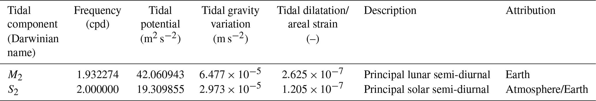
Figure 1 Representation of the groundwater level measured as pressure head in a well penetrating a confined aquifer with a rigid matrix subjected to ET (red) and AT (grey), adapted from McMillan et al. (2019). The result of these two effects can be expressed as a function of harmonic addition within the measured groundwater levels. The gravity-induced directional strain and vertical barometric loading combine to force water into and out of the well.

Three variables are required to calculate subsurface properties using specific harmonic components (McMillan et al., 2019): (1) a computed dilatation or strain due to ETs (denoted by the superscript “ET”); (2) measured barometric pressure (denoted by the superscript AT in later equations); and (3) measured groundwater heads (denoted by the superscript “GW”). First, a moving average spanning across a period of 3 d is applied. The tidally induced frequency components are then extracted by using HALS to estimate the harmonic components caused by tides whose frequencies are well known (Hsieh et al., 1987; Xue et al., 2016; Rau et al., 2020; Schweizer et al., 2021). The moving average acts like a high-pass filter and the extraction of the tidal components at specific frequencies means that lower-frequency and episodic events (atmospheric pressure changes related to weather systems passing across a site, rainfall and recharge events, and recession from pumping or droughts) present in the groundwater level or pressure data are discarded and therefore of no consequence for the analysis. Further, since our analysis is exclusively valid for the semi-confined and confined subsurface, water movement in the overlying shallow vadose zone and unconfined saturated zone is irrelevant. The extracted frequency components are complex numbers at discrete frequencies (${\widehat{z}}_{\left(\mathrm{f}\right)}$, e.g. ${\widehat{z}}_{M_{\mathrm{2}}}$) for which amplitudes and phases can be calculated using the real and imaginary parts. The approach we use in our work (e.g. HALS) was comprehensively tested showing that it leads to accurate estimates of harmonics in the presence of noise levels not exceeding the measurement resolution (Schweizer et al., 2021). High-quality pressure transducers generally fulfil this criterion (Rau et al., 2019).

2.2 Earth tide influences on well water levels

2.2.1 Subsurface strain response to gravity changes

Rojstaczer and Agnew (1989) argued that for ET, horizontal areal strain is a sufficient approximation for depths of up to thousands of kilometres. This approximation is therefore sufficient for application to groundwater resources as they are generally much shallower. The strain is often referred to as “dilatation”, which is the total increase in volume of the material due to forcing by the ET (in this case the tidal pull). In porous media, assuming incompressible grains, this dilatation manifests as an opening of the total pore space, decreasing the water pressure within the material (Agnew, 2010).

In this paper, we focus on the ET component at the frequency of 1.932274 cycles per day (cpd; denoted by a subscript of its Darwin name M₂) and the combined ET and AT component at the frequency of 2 cpd (denoted by a subscript of its Darwin name S₂), described in Table 1. While other frequency components can also be used (Hsieh et al., 1988; Merritt, 2004; Cutillo and Bredehoeft, 2011), M₂ and S₂ generally have the strongest tidal impact and their forces remain constant over time (Acworth et al., 2016; McMillan et al., 2019).

In this paper the term “dilatation” is used broadly to represent both the dilation and compression due to the cyclical forcing of the tides, consistent with its previous use in the literature (Xue et al., 2016; Allègre et al., 2016). The distortions by dilatation can be estimated through the planar strain concept known as “tidal dilatation” (Schulze et al., 2000; Fuentes-Arreazola et al., 2018). Tidal dilatation can be defined as

$$\begin{array}{}\text{(1)}& e={\displaystyle \frac{V}{g}}\cdot {\displaystyle \frac{e^{\mathrm{v}}-\mathrm{3}{e}^{\mathrm{h}}}{R}},\end{array}$$

where V is the tidal potential (m² s⁻²), M₂ is the tidal frequency, g is acceleration due to gravity (≈9.81 m s⁻²), e^v is vertical displacement (–), e^h is horizontal displacement (–) (Agnew, 2010), R the average radius of the Earth (m) adjusted for any significant elevation, and V is the tidal potential (m² s⁻²) as defined in Table 1. The term (e^v−3e^h) may also be approximated by Love–Shida numbers where e^v can be replaced by ${}_{\mathrm{S}}^{\mathrm{L}}h$ with an assumed value of 0.6032 and e^h may be replaced with ${}_{\mathrm{S}}^{\mathrm{L}}l$ with an assumed value of 0.0839 (Agnew, 2010; Cutillo and Bredehoeft, 2011). Previous work has demonstrated the use of theoretical ET when analysing the groundwater response (Roeloffs, 1996; Xue et al., 2016; Allègre et al., 2016; McMillan et al., 2019). The terms e^v and e^h can be directly calculated from software that generates theoretical ET potential (ET^pot) or tidal dilatation (e) or tidal strains (ET^ϵ) based on geo-location, for example ETERNA (Wenzel, 1996), TSoft (Van Camp and Vauterin, 2005), or, as was done for this paper, using PyGTide (Rau, 2018). This is based on ETERNA and uses the Wahr–Dehant–Zschau model which assumes an elliptical, rotating, inelastic, and oceanless Earth (Wahr, 1981; Dehant and Zschau, 1989).

The first approach using ET to estimate specific storage used the potential for water movement from the tides to the corresponding water movement in a monitoring well in a confined aquifer for undrained conditions. Here, Bredehoeft (1967) defined specific storage (S_s) for a medium that is presumed to be incompressible as

$$\begin{array}{}\text{(2)}& S_{\mathrm{s}}=-\left[\left({\displaystyle \frac{\mathrm{1}-\mathrm{2}\mathit{\nu }}{\mathrm{1}-\mathit{\nu }}}\right)\left({\displaystyle \frac{\mathrm{2}{h}_{\mathrm{S}}^{\mathrm{L}}-\mathrm{6}{l}_{\mathrm{S}}^{\mathrm{L}}}{R\cdot g}}\right)\right]{\displaystyle \frac{\mathrm{\Delta }{A}_{M_{\mathrm{2}}}^{{\mathrm{ET}}^{\mathrm{pot}}}}{\mathrm{\Delta }h}},\end{array}$$

where ν is the Poisson's ratio (generally assumed), $h_{\mathrm{S}}^{\mathrm{L}}$ and $l_{\mathrm{S}}^{\mathrm{L}}$ are dimensionless parameters describing Earth properties (Love–Shida numbers), and $\mathrm{\Delta }{A}_{M_{\mathrm{2}}}^{{\mathrm{ET}}^{\mathrm{pot}}}$ is the change in the tidal potential to the corresponding change in hydraulic head Δh. Here, the tidal dilatation (Eq. 1) has been incorporated into Eq. (2). Equation (2) was then used by Cutillo and Bredehoeft (2011) for is advantages over methods such as those provided by Hsieh et al. (1987), as it does not require the separation of individual tidal components or the knowledge of a well's dimensions. Progressive improvements in the precision and duration of gravity measurement methods have since allowed for more accurate decomposition and cataloguing of the various tidal components (Agnew, 2010). These established catalogues of precise frequencies provide the basis for component separation using harmonic filtering techniques. The full separation of ET and AT at one frequency enables their individual and combined use towards better in situ hydro-geomechanical characterisation (Rau et al., 2020).

We note that these codes do not account for ocean tide loading, i.e. the deformation of the subsurface due to the weight of the ocean tides. Ocean tide loading causes harmonic subsurface strain that is added to that imposed by ET. The actual subsurface strain amplitude variation depends on the phase of both signals and is, in the worst cases, either added to or subtracted from the ET. To understand the potential impact of this effect we used the ocean tide loading provided by Chalmers University of Technology (http://holt.oso.chalmers.se/loading/index.html, last access: 22 August 2022) to estimate the M₂ aerial strain amplitude for our five locations with the state-of-the-art finite element model FES2014b (Penna et al., 2008; Matviichuk et al., 2021). However, we further note that ocean tide loading is a complicated phenomenon (Jentzsch, 1997) and its detailed assessment is beyond the scope of this paper.

2.2.2 Well water level response to harmonically forced pore pressure

The relative amplitude response of the groundwater, as measured in a borehole in relation to the tidal dilatation or strain, can be expressed as (Hsieh et al., 1987; Xue et al., 2016; Allègre et al., 2016)

$$\begin{array}{}\text{(3)}& A_{M_{\mathrm{2}}}^{{\mathrm{ET}}^{\mathit{ϵ}}}=\left|{\displaystyle \frac{{\widehat{z}}_{M_{\mathrm{2}}}^{\mathrm{GW}}}{{\widehat{z}}_{M_{\mathrm{2}}}^{{\mathrm{ET}}^{\mathit{ϵ}}}}}\right|={\displaystyle \frac{A_{M_{\mathrm{2}}}^{\mathrm{GW}}}{A_{M_{\mathrm{2}}}^{{\mathrm{ET}}^{\mathit{ϵ}}}}},\end{array}$$

where ${\widehat{z}}_{M_{\mathrm{2}}}^{\mathrm{GW}}$ and ${\widehat{z}}_{M_{\mathrm{2}}}^{{\mathrm{ET}}^{\mathit{ϵ}}}$ are the complex frequency component of the groundwater pressure head and tidal strain, respectively; $A_{M_{\mathrm{2}}}^{\mathrm{GW}}$ is the amplitude of the groundwater pressure head fluctuation and $A_{M_{\mathrm{2}}}^{\mathit{ϵ}}$ is the amplitude of the tidal strain fluctuation, all at the frequency of the M₂ tidal component. Note that $A_{M_{\mathrm{2}}}^{{\mathrm{ET}}^{\mathit{ϵ}}}$ is also referred to as “areal strain sensitivity” (Hsieh et al., 1987).

It is important to note the difference presented in Eq. (3) from Xue et al. (2016) with the original dimensionless amplitude response calculated by Hsieh et al. (1987) as

$$\begin{array}{}\text{(4)}& A_{M_{\mathrm{2}}}=\left|{\displaystyle \frac{{\widehat{z}}_{M_{\mathrm{2}}}^{\mathrm{GW}}}{{\widehat{z}}_{M_{\mathrm{2}}}^{\mathrm{p}}}}\right|=A_{M_{\mathrm{2}}}^{{\mathrm{ET}}^{\mathit{ϵ}}}{S}_{\mathrm{s}},\end{array}$$

where ${\widehat{z}}_{M_{\mathrm{2}}}^{\mathrm{p}}$ is the complex aquifer pore pressure response (superscript “p” reflects pore). Here, the denominator term has changed from the complex amplitude of the pressure fluctuation to the tidal dilatation, effectively incorporating Eq. (2). This key difference allows for the addition of the storage term S_s within the amplitude response equations due to the sensitivity of storage to the amplitude response for confined and leaky responses described in Sect. 2.2.3 and 2.2.4. $A_{M_{\mathrm{2}}}$ from Eq. (4) is dimensionless, with values $\mathrm{0}\le A_{M_{\mathrm{2}}}\le \mathrm{1}$.

The phase shift (or phase difference) is defined as the strain response observed as the complex groundwater pressure head (water level) fluctuation, minus the phase of the complex tidal dilatation (tidal forcing) stress, defined as

$$\begin{array}{}\text{(5)}& \mathrm{\Delta }{\mathit{\varphi }}_{M_{\mathrm{2}}}=\arg \left({\displaystyle \frac{{\widehat{z}}_{M_{\mathrm{2}}}^{\mathrm{GW}}}{{\widehat{z}}_{M_{\mathrm{2}}}^{{\mathrm{ET}}^{\mathit{ϵ}}}}}\right)={\mathit{\varphi }}_{M_{\mathrm{2}}}^{\mathrm{GW}}-{\mathit{\varphi }}_{M_{\mathrm{2}}}^{{\mathrm{ET}}^{\mathit{ϵ}}},\end{array}$$

where ${\mathit{\varphi }}_{M_{\mathrm{2}}}^{\mathrm{GW}}$ is the phase angle expressed in the groundwater response and ${\mathit{\varphi }}_{M_{\mathrm{2}}}^{{\mathrm{ET}}^{\mathit{ϵ}}}$ is the phase angle of the theoretical ET component, in this case at the frequency of the M₂. A negative phase shift is expressed where the groundwater response lags behind the induced strain (i.e. water level response lags behind the pressure head disturbance; Hsieh et al., 1987), whereas a positive phase shift indicates the groundwater response is leading the strain response.

It should be noted that in this method development, a homogeneous, isotropic aquifer of infinite lateral extent is assumed for all derivations (Hsieh et al., 1987). All derived hydro-geomechanical variables are treated as bulk properties averaged over a distinct but unknown volume, representative of the EAT area of influence around the monitoring well screened interval, including effects from geological heterogeneities and the well construction, such as the inclusion of a gravel pack. The exact nature and dimensions of the volume of influence, i.e. the volume of subsurface around the well being “sampled”, is currently unresolved. It is commonly assumed that the ET amplitude response is negligibly influenced by fluid flow when the screened aquifer is confined (Xue et al., 2016). Instead, it is predominantly controlled by a change in storage. This is used as a justification to modify the hydraulic diffusivity term in the amplitude response equations to $\mathrm{1}/Ss$ when including the ET strain estimation (Eqs. 6 and 13), i.e. the tidal dilatation (Hsieh et al., 1987; Wang, 2000; Xue et al., 2016).

2.2.3 Confined water level response

Positive and negative phase shifts are either leading (leaky) or lagging (confined), respectively, in relation to the strain response expressed by the water level in a well to formation tidal forcing. Hsieh et al. (1987) provided an analytical solution for the confined groundwater flow equation with harmonic forcing to describe the relationship between aquifer pore pressure and well water level. Their model assumes horizontal flow only and is formulated in terms of amplitude ratio and phase shift, thereby allowing for the solution of two properties, transmissivity and storativity from the amplitude and phase response. The confined (negative phase) model is defined by Hsieh et al. (1988) as

$$\begin{array}{}\text{(6)}& A_{M_{\mathrm{2}}}={\displaystyle \frac{\mathrm{1}}{\sqrt{\left(E^{\mathrm{2}}+F^{\mathrm{2}}\right)}}}\end{array}$$

and

$$\begin{array}{}\text{(7)}& \mathrm{\Delta }{\mathit{\varphi }}_{M_{\mathrm{2}}}=-{\tan }^{-\mathrm{1}}\left({\displaystyle \frac{F}{E}}\right)\end{array}$$

with the following parameters:

$$\begin{array}{}\text{(8)}& E=\mathrm{1}-{\displaystyle \frac{\mathit{\omega }{r}_{\mathrm{c}}^{\mathrm{2}}}{\mathrm{2}T}}\left[\mathrm{\Psi }\mathrm{Ker}\left({\mathit{\alpha }}_{\mathrm{w}}\right)+\mathit{\psi }\mathrm{Kei}\left({\mathit{\alpha }}_{\mathrm{w}}\right)\right]\end{array}$$

and

$$\begin{array}{}\text{(9)}& F={\displaystyle \frac{\mathit{\omega }{r}_{\mathrm{c}}^{\mathrm{2}}}{\mathrm{2}T}}\left[\mathit{\psi }\mathrm{Ker}\left({\mathit{\alpha }}_{\mathrm{w}}\right)-\mathrm{\Psi }\mathrm{Kei}\left({\mathit{\alpha }}_{\mathrm{w}}\right)\right].\end{array}$$

These include

$$\begin{array}{}\text{(10)}& \mathrm{\Psi }={\displaystyle \frac{-\left[{\mathrm{Ker}}_{\mathrm{1}}\left({\mathit{\alpha }}_{\mathrm{w}}\right)-{\mathrm{Kei}}_{\mathrm{1}}\left({\mathit{\alpha }}_{\mathrm{w}}\right)\right]}{\sqrt{\mathrm{2}}\left[{\mathrm{Ker}}_{\mathrm{1}}^{\mathrm{2}}\left({\mathit{\alpha }}_{\mathrm{w}}\right)+{\mathrm{Kei}}_{\mathrm{1}}^{\mathrm{2}}\left({\mathit{\alpha }}_{\mathrm{w}}\right)\right]{\mathit{\alpha }}_{\mathrm{w}}}}\end{array}$$

and

$$\begin{array}{}\text{(11)}& \mathit{\psi }={\displaystyle \frac{-\left[{\mathrm{Ker}}_{\mathrm{1}}\left({\mathit{\alpha }}_{\mathrm{w}}\right)+{\mathrm{Kei}}_{\mathrm{1}}\left({\mathit{\alpha }}_{\mathrm{w}}\right)\right]}{\sqrt{\mathrm{2}}\left[{\mathrm{Ker}}_{\mathrm{1}}^{\mathrm{2}}\left({\mathit{\alpha }}_{\mathrm{w}}\right)+{\mathrm{Kei}}_{\mathrm{1}}^{\mathrm{2}}\left({\mathit{\alpha }}_{\mathrm{w}}\right)\right]{\mathit{\alpha }}_{\mathrm{w}}}},\end{array}$$

where

$$\begin{array}{}\text{(12)}& {\mathit{\alpha }}_{\mathrm{w}}=r_{\mathrm{w}}\sqrt{{\displaystyle \frac{\mathit{\omega }S}{T}}}=r_{\mathrm{w}}\sqrt{{\displaystyle \frac{\mathit{\omega }}{D_{\mathrm{h}}}}}.\end{array}$$

Here, Ker, Kei and Ker₁, Kei₁ are the real and imaginary parts of the Kelvin function of order 0 and 1, respectively. The storativity S and transmissivity T can be related to specific storage as S=S_sb and hydraulic conductivity as T=k^fb, respectively; b is the aquifer thickness, which when the aquifer thickness is unknown is approximated with the vertical screen length; r_w is the internal radius of the well screen (accounts for well storage); r_c is the outer radius of the casing. Ker and Kei are Kelvin functions of zero order, and Ker₁ and Kei₁ are Kelvin functions of the first order. Figure 2a and b show the amplitude and phase solution space when considering the strain response as well as separation of hydraulic properties.

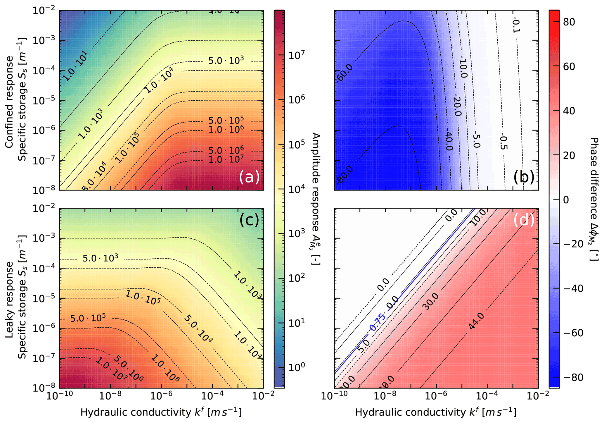
Figure 2 Pressure head amplitude and phase response to the Earth tide M₂ component as a function of ranges in hydraulic conductivity and specific storage: (a) amplitude response (Eq. 6) and (b) phase shift (Eq. 7) for confined conditions (the radius of the borehole and screen is 0.1 m and the screen length is 2 m). (c) Amplitude response (Eq. 13) and (d) phase shift (Eq. 14) for semi-confined conditions with vertical flow (the depth of the screen is 20 m).

2.2.4 Leaky water level response

The leaky water level model is based on the description of a periodic load on a half-space, as described by Wang (2000), and is used for ET where a vertical pressure propagation and flow exist (Xue et al., 2016; Allègre et al., 2016). Equations (13) and (14) were derived from the force equilibrium equations (refer to Wang, 2000)

$$\begin{array}{}\text{(13)}& A_{M_{\mathrm{2}}}=\sqrt{\mathrm{1}-\mathrm{2}\exp \left(-{\displaystyle \frac{z}{\mathit{\delta }}}\right)\cos \left({\displaystyle \frac{z}{\mathit{\delta }}}\right)+\exp \left(-\mathrm{2}{\displaystyle \frac{z}{\mathit{\delta }}}\right)},\end{array}$$

and

$$\begin{array}{}\text{(14)}& \mathrm{\Delta }{\mathit{\varphi }}_{M_{\mathrm{2}}}={\tan }^{-\mathrm{1}}\left[{\displaystyle \frac{\exp \left(-\frac{z}{\mathit{\delta }}\right)\sin \left(\frac{z}{\mathit{\delta }}\right)}{\mathrm{1}-\exp \left(-\frac{z}{\mathit{\delta }}\right)\cos \left(\frac{z}{\mathit{\delta }}\right)}}\right],\end{array}$$

where z is depth of the midpoint open screen interval, ω is the angular frequency of the tidal component (M₂), and

$$\begin{array}{}\text{(15)}& \mathit{\delta }=\sqrt{{\displaystyle \frac{\mathrm{2}{D}_{\mathrm{h}}}{\mathit{\omega }}}}.\end{array}$$

Here, D_h is then the hydraulic diffusivity, defined as

$$\begin{array}{}\text{(16)}& D_{\mathrm{h}}={\displaystyle \frac{T}{S}}={\displaystyle \frac{k^{\mathrm{f}}}{S_{\mathrm{s}}}}={\displaystyle \frac{k}{\mathit{\mu }S}}={\displaystyle \frac{{\mathit{\rho }}_{\mathrm{w}}g{k}^{\mathrm{f}}}{\mathit{\mu }{S}_{\mathrm{s}}}},\end{array}$$

where T is the transmissivity (T=k^fb), k is permeability, k^f is hydraulic conductivity, ρ_w is the density of water (0.9982 kg L⁻¹ at 20 ^∘C), μ is the dynamic viscosity of water (8.90×10⁻⁴ Pa s), and S is storativity. Equations (13) and (14) require iterative solving for D_h and S_s.

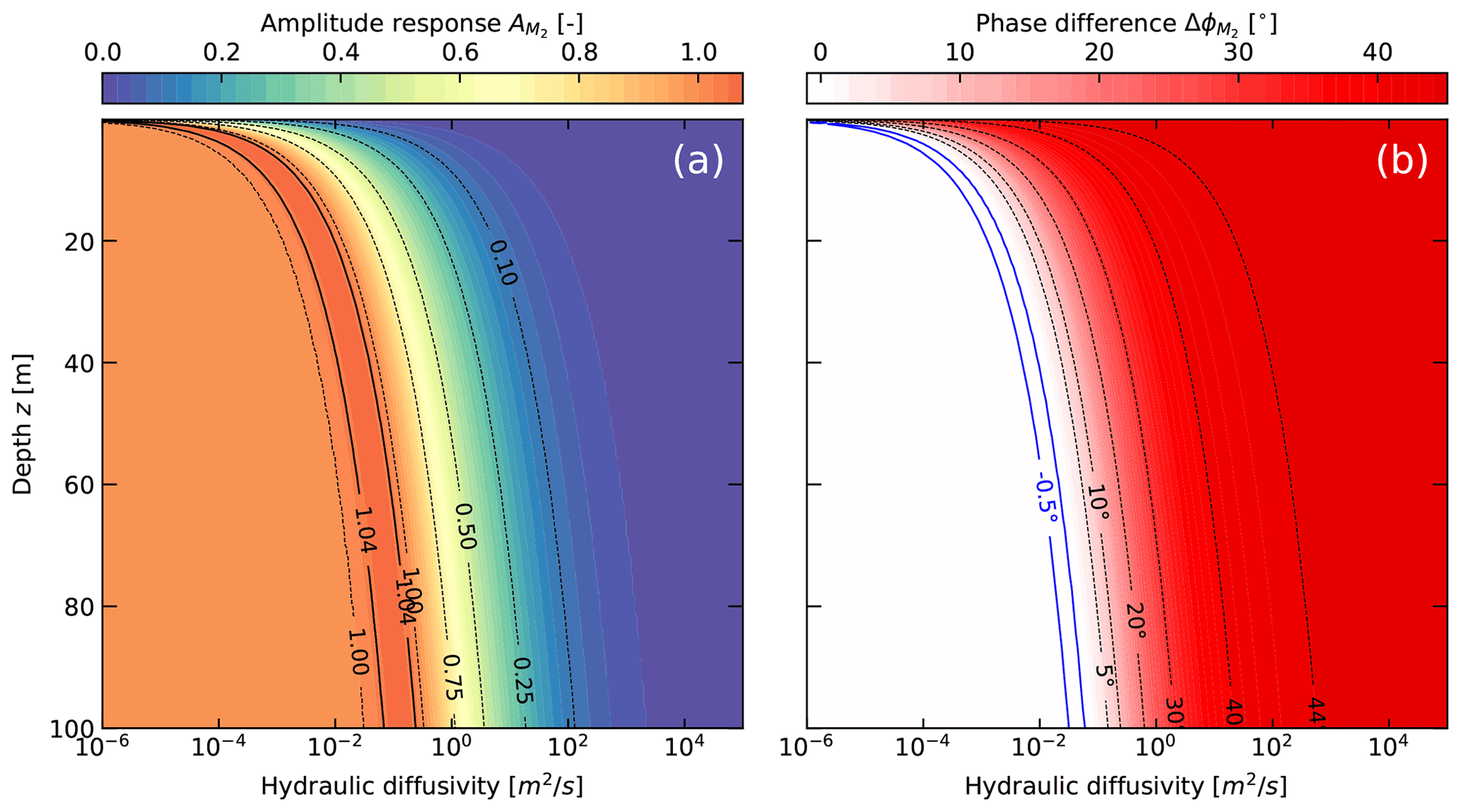
Figure 3 shows the solution space for Eqs. (13) and (14). It is noteworthy that the amplitude can be attenuated significantly for high hydraulic diffusivities and shallow depths. Overall, confined conditions should prevail for low hydraulic diffusivities and larger depths where the amplitude ratio is ≈1. Semi-confined conditions are indicated by positive phase shifts. Note that hydraulic diffusivities in the range of ∼0.01–0.1 (m² s) can increase the amplitudes to approx. 1.07 (Fig. 3a) for which phase shifts can assume negative values (e.g. −0.5^∘ in Fig. 3b). Figure 2c and d show the solution space when considering the strain response as well as separation of hydraulic properties for leaky conditions.

Figure 3 Periodic loading of a half space (applied to ET) as represented by Eqs. (13) and (14). (a) Normalised amplitude response as a function of hydraulic diffusivity and depth (Eq. 13). (b) Phase response as a function of depth and hydraulic diffusivity (Eq. 14) (Wang, 2000).

2.2.5 Distinguishing between leaky and confined conditions

The sets of Eqs. (6) and (7) (Hsieh et al., 1987) describe lateral water movement between the well bore and surrounding subsurface, whereas Eqs. (13) and (14) (Wang, 2000) explain the positive phase shift by allowing vertical flow within the groundwater system. Both sets of equations have been used to estimate hydraulic conductivity and specific storage. This is achieved by decomposing the hydraulic diffusivity using the assumptions outlined at the end of Sect. 2.2.2.

The phase shift determines which of these sets of analytical solutions are appropriate. For a phase shift of $-\mathrm{45}{}^{\circ }\le \mathrm{\Delta }{\mathrm{\Phi }}_{M_{\mathrm{2}}}<\mathrm{0}{}^{\circ }$, the confined response model is used, and for a phase shift of $\mathrm{0}\le \mathrm{\Delta }{\mathrm{\Phi }}_{M_{\mathrm{2}}}\le \mathrm{90}{}^{\circ }$, the leaky response model is applied (both are illustrated in Fig. 2). Note that the leaky model may result in a slight negative phase shift for certain parameter ranges. Consequently, there is a range of ambiguity in phase shift values between −1 and 0^∘ in which both sets of solutions should be used, and the most physically plausible results should be selected (Xue et al., 2016). Note, the unit input as either pressure or hydraulic head will also be carried through the equations resulting in a unit difference where $S_{\mathrm{s}}^{\mathrm{p}}$ is specific storage expressed in 1 Pa⁻¹ whereas S_s is specific storage expressed as 1 m⁻¹, as demonstrated in Eq. (16).

2.3 Atmospheric tide influences on well water levels

Methods that quantify the barometric efficiency of subsurface systems are based on quantifying the groundwater response magnitude to atmospheric pressure changes (Clark, 1967; Rasmussen and Crawford, 1997; Barr et al., 2000; Gonthier, 2003) or atmospheric tides (Acworth et al., 2016). Turnadge et al. (2019) reviewed these methods and concluded that the method by Acworth et al. (2016) was the most robust and reliable. However, their approach was limited by the assumption of an instantaneous and undamped response. Rau et al. (2020) developed a new method that completely disentangles the influences of EAT at the same frequency, e.g. S₂. This further considers the damping of the amplitude that can be caused by low hydraulic conductivity materials under confined conditions (Sect. 2.2.3) or attenuation of the amplitude under semi-confined conditions (Sect. 2.2.4). Their new approach is (Rau et al., 2020)

$$\begin{array}{}\text{(17)}& {\mathrm{BE}}_{S_{\mathrm{2}}}={\displaystyle \frac{\mathrm{1}}{A_{M_{\mathrm{2}}}}}\cdot \left|{\displaystyle \frac{{\widehat{z}}_{S_{\mathrm{2}}}^{\mathrm{GW}\cdot \mathrm{AT}}}{{\widehat{z}}_{S_{\mathrm{2}}}^{\mathrm{AT}}}}\right|,\end{array}$$

where

$$\begin{array}{}\text{(18)}& {\widehat{z}}_{S_{\mathrm{2}}}^{\mathrm{GW}\cdot \mathrm{AT}}={\widehat{z}}_{S_{\mathrm{2}}}^{\mathrm{GW}}-{\widehat{z}}_{S_{\mathrm{2}}}^{\mathrm{GW}\cdot \mathrm{ET}}={\widehat{z}}_{S_{\mathrm{2}}}^{\mathrm{GW}}-{\displaystyle \frac{{\widehat{z}}_{M_{\mathrm{2}}}^{\mathrm{GW}}}{{\widehat{z}}_{M_{\mathrm{2}}}^{\mathrm{ET}}}}{\widehat{z}}_{S_{\mathrm{2}}}^{\mathrm{ET}}.\end{array}$$

Here, $A_{M_{\mathrm{2}}}$ corrects for the damping of the subsurface-well system and can be inferred from ET (Eq. 4) for confined conditions, e.g. for low hydraulic conductivity (Eq. 6), or damping under semi-confined conditions (Eq. 13). ${\widehat{z}}_{S_{\mathrm{2}}}^{\mathrm{GW}\cdot \mathrm{AT}}$ is the S₂ component of the groundwater response to AT, and ${\widehat{z}}_{S_{\mathrm{2}}}^{\mathrm{AT}}$ is the S₂ frequency component (AT) embedded in atmospheric pressure measurements. ${\widehat{z}}_{S_{\mathrm{2}}}^{\mathrm{GW}\cdot \mathrm{ET}}$ is the S₂ component of the groundwater response to Earth tides (e.g., potential or strain). BE forms a stress balance, described as (Jacob, 1940)

$$\begin{array}{}\text{(19)}& \mathrm{BE}+\mathit{\gamma }=\mathrm{1},\end{array}$$

where γ is the loading efficiency.

2.4 Combining ET and AT responses

2.4.1 General relationships

Within the following derivations it is assumed that ET only induce horizontal areal strain (${\mathit{ϵ}}_{xy}={\mathit{ϵ}}_x+{\mathit{ϵ}}_y$) whereas AT only induce vertical strain (${\mathit{ϵ}}_z=-p^{\mathrm{AT}}$) (Rojstaczer and Agnew, 1989; Cutillo and Bredehoeft, 2011), all of which are assumed to act instantaneously on the subsurface as is consistent with previous literature (Wang, 2000; Rau et al., 2018). Under such conditions, van der Kamp and Gale (1983) has shown that the rigidity modulus (also known as “the shear modulus”, G) can be estimated, with the previous outlined assumptions, from combined ET and AT influences as

$$\begin{array}{}\text{(20)}& G=A_{M_{\mathrm{2}}}^{{\mathrm{ET}}^{\mathit{ϵ}}}{\displaystyle \frac{\mathit{\rho }g}{\mathrm{2}\mathit{\gamma }}}=A_{M_{\mathrm{2}}}^{{\mathrm{ET}}^{\mathit{ϵ}}}{\displaystyle \frac{\mathit{\rho }g}{\mathrm{2}(\mathrm{1}-\mathrm{BE})}},\end{array}$$

where, $A_{M_{\mathrm{2}}}^{{\mathrm{ET}}^{\mathit{ϵ}}}$ originates from ET (Eq. 3), whereas BE or γ is derived from AT (Eq. 19).

The disentanglement of ET and AT from the groundwater level response in a well, and the subsequent use of these separate frequency components to quantify hydro-geomechanical properties, allows further geomechanical derivations to be made. Two methods are presented below which solve for the assumption of either incompressible (suitable for unconsolidated material) or compressible grains (suitable for consolidated material). The choice between which method to use is established by examining an estimated Biot–Willis coefficient defined as (Wang, 2000)

$$\begin{array}{}\text{(21)}& \mathit{\alpha }=\mathrm{1}-{\displaystyle \frac{K}{K_{\mathrm{s}}}}=\mathrm{1}-{\displaystyle \frac{{\mathit{\beta }}_{\mathrm{s}}}{\mathit{\beta }}},\end{array}$$

where K is the bulk modulus, K_s is the bulk modulus of the solid grain, β is the compressibility, and β_s is the compressibility of the solid grain. For unconsolidated conditions, where the bulk modulus is much smaller than the bulk modulus of the grains (K≪K_s), it is possible to assume that the grains do not contribute to the overall compressibility, thus the grains are incompressible. The Biot–Willis coefficient α→1 shows that the contribution of the grains to the compressibility of the bulk material is insignificant (Rau et al., 2018). By contrast, in consolidated cases K becomes larger, leading to a coefficient that deviates appreciably from 1 (α<1). In such cases, the grain compressibility is a significant proportion of the total material compressibility and must be accounted for.

2.4.2 Unconsolidated systems

In unconsolidated systems, the compressibility of the grains is much smaller than that of the bulk leading to α=1. This enables simplification of the theory. In the following, undrained parameters are indicated by the superscript “u”. The uniaxial loading efficiency is related to the uniaxial bulk properties as (van der Kamp and Gale, 1983)

$$\begin{array}{}\text{(22)}& \mathit{\gamma }={\displaystyle \frac{{\mathit{\beta }}_{\mathrm{v}}^{\mathrm{u}}}{\mathit{\theta }{\mathit{\beta }}_{\mathrm{f}}+{\mathit{\beta }}_{\mathrm{v}}^{\mathrm{u}}}},\end{array}$$

where β_f is the compressibility of the fluid ($\mathrm{4.59}\times {\mathrm{10}}^{-\mathrm{10}}$ Pa⁻¹ at 20 ^∘C), ${\mathit{\beta }}_{\mathrm{v}}^{\mathrm{u}}$ is the vertical undrained bulk compressibility, and θ is the total porosity of the formation. The uniaxial specific storage (assuming incompressible grains) is defined by Jacob (1940) as

$$\begin{array}{}\text{(23)}& S_{\mathrm{s}}={\mathit{\rho }}_{\mathrm{w}}g\left({\mathit{\beta }}_{\mathrm{v}}^{\mathrm{u}}+\mathit{\theta }{\mathit{\beta }}_{\mathrm{f}}\right).\end{array}$$

Acworth et al. (2016) used Eq. (22) to simplify Eq. (23) as follows:

$$\begin{array}{}\text{(24)}& S_{\mathrm{s}}={\mathit{\rho }}_{\mathrm{w}}g{\mathit{\beta }}_{\mathrm{f}}{\displaystyle \frac{\mathit{\theta }}{\mathrm{BE}}}=\mathrm{4.5}\times {\mathrm{10}}^{-\mathrm{6}}{\displaystyle \frac{\mathit{\theta }}{\mathrm{BE}}}.\end{array}$$

However, this requires a prior estimate of the porosity θ, which is often difficult to determine due to the lack of independent measurements.

Note that the above equations assume that barometric loading is uniaxial, and as such use vertical compressibility (${\mathit{\beta }}_{\mathrm{v}}^{\mathrm{u}}$) rather than the volumetric (bulk) compressibility (β^u). Here, we instead propose using the S_s derived from the response to ET (Sect. 2.2) to estimate the subsurface porosity by rearranging Eq. (24) (similar to Jacob, 1940) as

$$\begin{array}{}\text{(25)}& \mathit{\theta }={\displaystyle \frac{S_{\mathrm{s}}\mathrm{BE}}{{\mathit{\rho }}_{\mathrm{w}}g{\mathit{\beta }}_{\mathrm{f}}}}={\displaystyle \frac{S_{\mathrm{s}}}{{\mathit{\rho }}_{\mathrm{w}}g{\mathit{\beta }}_{\mathrm{f}}}}(\mathrm{1}-\mathit{\gamma }).\end{array}$$

To achieve a similar outcome as Acworth et al. (2016) this porosity, in addition to the calculated S_s, can also be used to provide a uniaxial (vertical) bulk compressibility (inverse vertical undrained bulk modulus ($K_{\mathrm{v}}^{\mathrm{u}}$)) of the subsurface defined as (Acworth et al., 2016)

$$\begin{array}{}\text{(26)}& {\mathit{\beta }}_{\mathrm{v}}^{\mathrm{u}}={\displaystyle \frac{\mathrm{1}}{K_{\mathrm{v}}^{\mathrm{u}}}}=\mathit{\theta }{\mathit{\beta }}_{\mathrm{f}}{\displaystyle \frac{\mathit{\gamma }}{\mathrm{1}-\mathit{\gamma }}}.\end{array}$$

This approach is similar to the one of Cutillo and Bredehoeft (2011) but uses the objective BE method developed by Rau et al. (2020) instead of the subjective correlation by Gonthier (2003). In this subsection it has been shown that it is possible to derive an estimate of porosity from a loading strain if the specific storage is known. This assumes incompressible grains (α≈1) and is therefore applicable for unconsolidated materials (Rau et al., 2019).

The assumption of incompressible grains allows for the removal of the grain compressibility and provides a simplification of the poroelastic parameter space. This step combined with the new derivation of the shear modulus enables a linear analytical solution of the remaining elastic variables in unconsolidated material (α≈1). The first step can be taken by deriving the undrained bulk modulus (K_u) with the $K_{\mathrm{v}}^{\mathrm{u}}$ from Acworth et al. (2016) as (Wang, 2000)

$$\begin{array}{}\text{(27)}& K^{\mathrm{u}}=K_{\mathrm{v}}^{\mathrm{u}}-{\displaystyle \frac{\mathrm{4}}{\mathrm{3}}}G,\end{array}$$

which makes it possible to solve the Skempton coefficient defined as (Rau et al., 2018)

$$\begin{array}{}\text{(28)}& B=\mathit{\gamma }{\displaystyle \frac{K_{\mathrm{v}}^{\mathrm{u}}}{K^{\mathrm{u}}}}=\mathit{\gamma }{\displaystyle \frac{{\mathit{\beta }}^{\mathrm{u}}}{{\mathit{\beta }}_{\mathrm{v}}^{\mathrm{u}}}}.\end{array}$$

Determination of the Skempton coefficient along with the loading efficiency unlocks the undrained Poisson's ratio using (Wang, 2000)

$$\begin{array}{}\text{(29)}& {\mathit{\nu }}^{\mathrm{u}}={\displaystyle \frac{\mathrm{3}\mathit{\gamma }-B}{\mathrm{3}\mathit{\gamma }+B}}\end{array}$$

and drained Poisson's ratio as (Wang, 2000)

$$\begin{array}{}\text{(30)}& \mathit{\nu }={\displaystyle \frac{\mathrm{3}{\mathit{\nu }}^{\mathrm{u}}-B\left(\mathrm{1}+{\mathit{\nu }}^{\mathrm{u}}\right)}{\mathrm{3}-\mathrm{2}B\left(\mathrm{1}+{\mathit{\nu }}^{\mathrm{u}}\right)}}.\end{array}$$

Determination of the drained Poisson ratio further unlocks all remaining poroelastic properties such as Young's modulus (E), defined as (Wang, 2000)

$$\begin{array}{}\text{(31)}& E={\displaystyle \frac{\mathrm{9}KG}{\mathrm{3}K+G}}.\end{array}$$

Equations (22)–(31) define the complete parameter space for unconsolidated materials.

2.4.3 Consolidated systems

To determine the poroelastic properties of consolidated materials, the grain compressibility must be considered leading to α<1. Further, the following two assumptions must be made: (1) although pore fluids technically respond to cubic strains, the areal strain can be used to estimate the subsurface strain from ET; (2) the system is homogeneous and laterally extensive, thus ignoring topographic effects and considering the barometric loading to be uniform. The equations that define the remaining elastic properties for such conditions are (Beavan et al., 1991) Skempton's constant

$$\begin{array}{}\text{(32)}& B={\displaystyle \frac{\mathrm{3}\mathit{\gamma }(\mathrm{1}-\mathit{\nu })}{\mathrm{2}\mathit{\gamma }\mathit{\alpha }(\mathrm{1}-\mathrm{2}\mathit{\nu })+(\mathrm{1}+\mathit{\nu })}},\end{array}$$

the total porosity

$$\begin{array}{}\text{(33)}& \mathit{\theta }=\left({\displaystyle \frac{\mathrm{1}}{B}}-\mathrm{1}\right)\left({\displaystyle \frac{\mathrm{1}}{K}}-{\displaystyle \frac{\mathrm{1}}{K_{\mathrm{s}}}}\right){\left({\displaystyle \frac{\mathrm{1}}{k^{\mathrm{f}}}}-{\displaystyle \frac{\mathrm{1}}{K_{\mathrm{s}}}}\right)}^{-\mathrm{1}},\end{array}$$

the Biot–Willis coefficient

$$\begin{array}{}\text{(34)}& \mathit{\alpha }=\mathrm{1}-{\displaystyle \frac{K}{K_{\mathrm{s}}}}=\mathrm{1}-{\displaystyle \frac{\mathrm{2}G(\mathrm{1}+\mathit{\nu })}{\mathrm{3}{K}_{\mathrm{s}}(\mathrm{1}-\mathrm{2}\mathit{\nu })}},\end{array}$$

and the specific storage

$$\begin{array}{}\text{(35)}& S_{\mathrm{s}}={\displaystyle \frac{\mathit{\rho }g}{\mathit{\gamma }(\mathrm{1}-\mathit{\nu })}}\left({\displaystyle \frac{\mathrm{1}-\mathrm{2}\mathit{\nu }}{\mathrm{2}G}}-{\displaystyle \frac{\mathrm{1}+\mathit{\nu }}{\mathrm{3}{K}_{\mathrm{s}}}}\right).\end{array}$$

Equations (32)–(35) form a non-linear system which must be solved by iteration.

If the petrology of the lithology is known, appropriate literature compressibility values of the dominant grain mineralogy (K_s) could be used. Quartz is the most common naturally occurring mineral and is also one of the least compressible (it is also applicable for most of our case sites), and it will therefore be used to define the upper bounds of K_s here. Richardson et al. (2002) summarised literature values of poly-crystalline quartz for K_s to range between 36 and 40 GPa, and reported K_s values for the quartz Ottawa Sandstone to be in a range of 30–50 GPa. The average of these ranges has been summarised as 42 GPa (Rau et al., 2018) and will be used in this work.

With the established inputs of γ(BE), $A_{M_{\mathrm{2}}}$, G (Eq. 20), S_s, and an estimate of K_s, it is possible to simultaneously solve Eqs. (32)–(35) for Skempton's coefficient (B), porosity (θ), and Biot–Willis coefficient (α) (Beavan et al., 1991). This enables a complete calculation of all remaining poroelastic properties using the relationships that can be found in Wang (2000).

3 Examples of method applications

3.1 Field sites, datasets, and interpretation

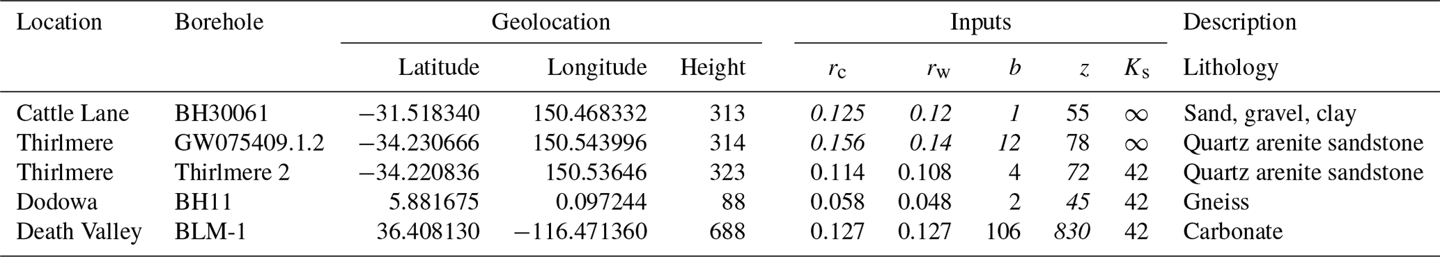
To demonstrate the new method, groundwater and barometric pressure records from four field sites and five monitoring bores were used. These sites were selected based on three main criteria: (1) data availability and quality; (2) a significant groundwater response to ET (M₂); (3) providing a variety of hydrogeological settings with existing studies for parameter comparisons. Further details about each site are described in separate sections below. Specific bore geometries and measurements used in the analysis of these sites, such as depths and bore construction, casing and screen radius as well as screen depth and length, are summarised in Table 2.

Table 2 Input parameters for case sites where r_c is the outer diameter (m) of the bore casing, r_w the internal diameter (m) of the bore casing, b is the Aquifer thickness (m) or open interval of the screen, z is the depth (m) to the centre of the screen or open bore interval, and K_s is the assumed grain bulk modulus. Italicised values were not used in the applied leaky or confined models, but are provided for completeness and context.

Groundwater pressure head and barometric pressure time series were recorded at sub-hourly intervals at all sites (e.g. two sites shown in Fig. 4) for at least 3 months, which is longer than the ∼28 d being suggested as the minimum requirement of the HALS method used here (Schweizer et al., 2021). Geo-position of the boreholes, theoretical ET strain for the same duration, and sampling frequency of each site as well as aerial strain amplitudes from ocean tide loading for M₂ are summarised in Table 2.

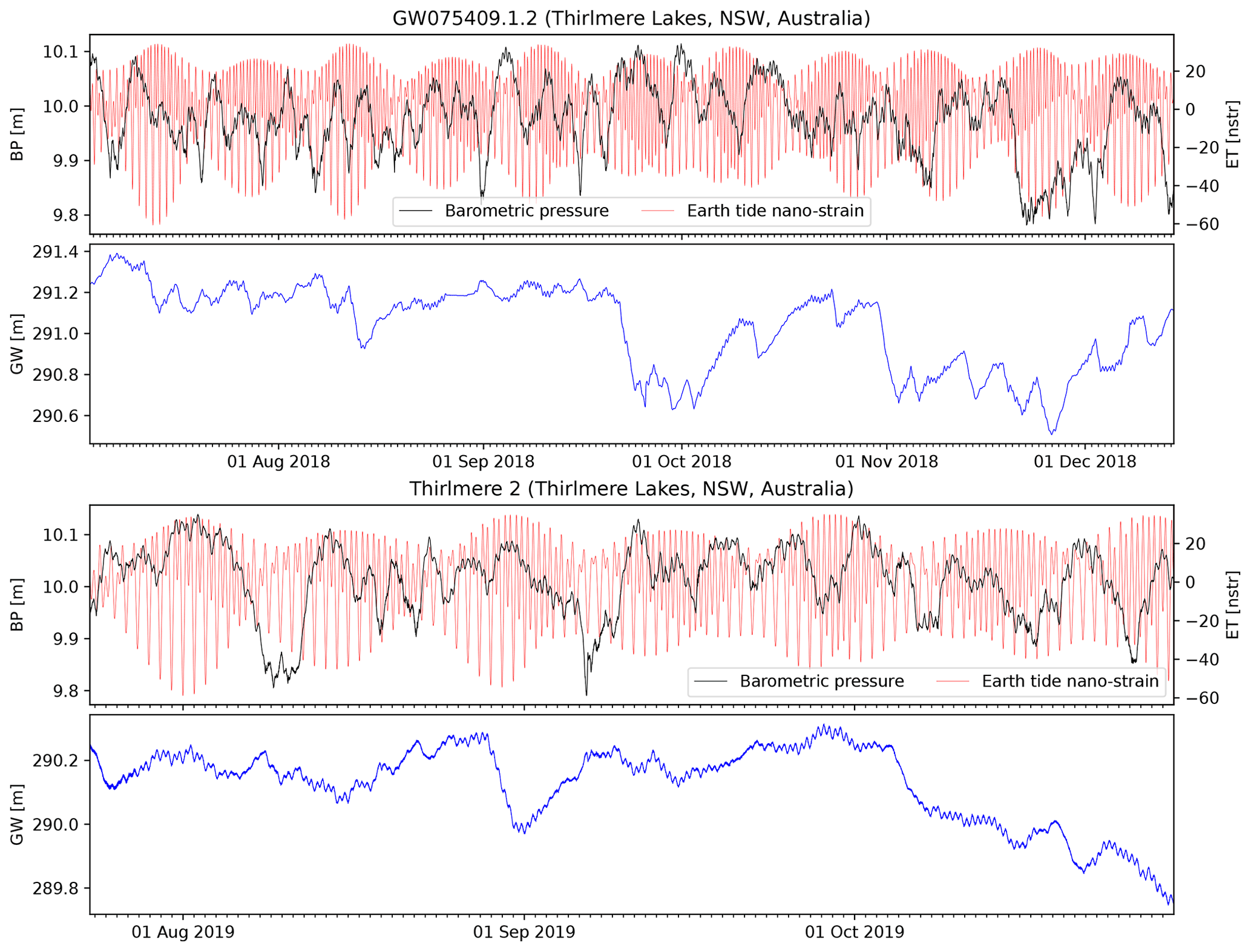
Figure 4 Time series of groundwater levels from bores GW075409.1.2 and Thirlmere 2 located at Thirlmere Lakes (NSW, Australia), barometric pressures (in metre-equivalent water heights for easier comparison to the groundwater pressure heads), corresponding theoretical Earth tides (in nano-strain, nstr) calculated using PyGTide.

All time series were detrended by fitting a linear function through a moving 3 d window using the SciPy detrend function, and the main tidal components were extracted using HALS (Sect. 2.1). Tables 3 and 4 present the estimated hydro-geomechanical properties for all the field sites and are discussed in the sections below.

Table 3 Hydraulic results where $A_{M_{\mathrm{2}}}^{{\mathrm{ET}}^{\mathit{ϵ}}}$ is the Earth tide nano-strain amplitude (nstr), $A_{M_{\mathrm{2}}}^{{\mathrm{OT}}^{\mathit{ϵ}}}$ is the ocean tide strain amplitude (nstr), $A_{M_{\mathrm{2}}}^{\mathit{ϵ}}$ is the strain response amplitude (m per nstr), $A_{M_{\mathrm{2}}}$ is the amplitude ratio (–), $\mathrm{\Delta }{\mathrm{\Phi }}_{M_{\mathrm{2}}}$ is the phase shift (degrees), $<K>$ is hydraulic conductivity (m s⁻¹), S_s is the specific storage (1 m⁻¹), and BE is the barometric efficiency (–).

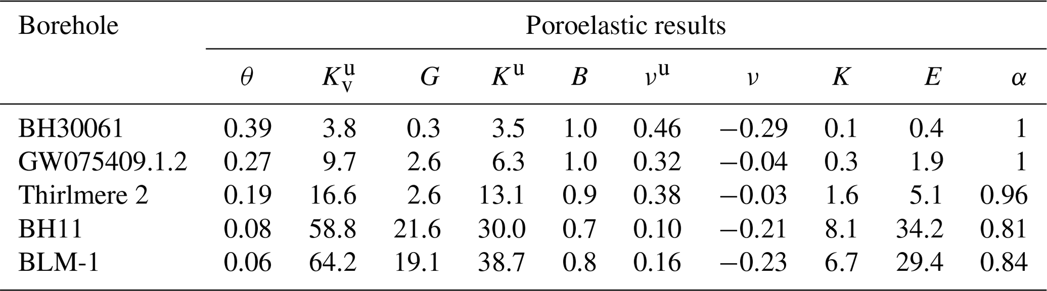
Table 4 Poroelastic results where θ is porosity (–), $K_{\mathrm{v}}^{\mathrm{u}}$ is the vertical undrained bulk modulus, G is the shear modulus (GPa), K^u is the undrained bulk modulus, B is Skempton's coefficient (–), ν^u is the undrained Poisson's Ratio (–), ν is Poisson's ratio (–), K is bulk modulus (GPa), E is Young's modulus (GPa), and α is the Biot–Willis coefficient (–).

In this paper, all of the methodology and equations were implemented in the Python programming language, and joint iterative solving was completed using SciPy's least-squares functionality. The following realistic parameter bounds were considered during root finding: $\mathrm{0}\le B\le \mathrm{1}$, $-\mathrm{1}\le \mathit{\nu }\le \mathrm{0.5}$, $\mathrm{0.005}\le G\le \mathrm{40}$ GPa, $\mathrm{0}\le \mathit{\theta }\le \mathrm{0.5}$. We note that (1) the parameter units were scaled to avoid bias towards parameters with large values, (2) the solver was set to 64-bit machine precision (epsilon $\sim \mathrm{1.11}\times {\mathrm{10}}^{-\mathrm{16}}$), and (3) none of the estimated parameters reached or exceeded any of the prescribed solution constraints.

3.2 Cattle Lane (NSW, Australia)

Cattle Lane is located on the Liverpool Plains, NSW, eastern Australia. Erosion of the basaltic Liverpool Range to the south produced a succession of unconsolidated silts, clays, sands, gravel, and minor carbonate nodules within the Liverpool Plains. A thick sequence of clay-bound sediments overlie a gravel aquifer at 40 m. This aquifer has previously be shown to respond to loading by rainfall events (Timms and Acworth, 2005). The lithology of the 1 m screened interval was described by Acworth et al. (2015) as major basalt fragments mixed with coarse sand, shell, and carbonate nodules. The site has previously been cored to 31.5 m depth, lithologically logged and geophysically surveyed, confirming that it is horizontally extensive (Acworth et al., 2015). Cross-hole seismics were also conducted by Rau et al. (2018) to the depth of 40 m (the screened interval of bore BH30061 is at 55 m depth, see Table 2), providing depth profiles of seismically inferred elastic variables that were used to constrain the pore pressure response to atmospheric tides analysis.

Further studies at this site include Acworth et al. (2016) and Acworth et al. (2017), which were precursors to Rau et al. (2018) in the investigation of pore pressure response to atmospheric tides, and Timms et al. (2018) on a core scale analysis of the site's laterally extensive and thick aquitard. Due to the sufficient M₂ response, time series data of groundwater pressure heads measured between 21 January 2016 and 14 April 2018 were used from bore BH30061. The groundwater pressure heads were collected using vented In-Situ Troll 700H series loggers at hourly intervals and sub-millimetre precision. Atmospheric pressure was measured by an In-Situ Baro Troll absolute gauge transducer.

The borehole BH30061 from Cattle Lane produced positive M₂ phase shifts (Table 2), with specific storage and hydraulic conductivity therefore being derived from the leaky model (Sect. 2.2.4). When applying the grain compressibility of quartz (K=42 GPa) a Biot–Willis coefficient of 0.99 is obtained and hence justifies the assumption of incompressible grains (α≈1) and the unconsolidated analytical model (Sect. 2.4.2).

The specific storage, hydraulic conductivity, porosity, shear modulus, and undrained Poisson's ratio from Cattle Lane are consistent with literature values for the sediment type (Bowles, 1996), and comply with previous estimates from higher in the stratigraphy at the same site obtained by cross-hole seismics (Acworth et al., 2015, 2016; Rau et al., 2018). Young's modulus of 0.4 GPa deviates from the expected material range reported in the literature for an unconsolidated clay, sand, and gravel mixture of between 0.025 and 0.2 GPa, although the obtained value is reasonable when considering the degree of consolidation at 55 m depth and the in situ determination rather than those obtained from laboratory tests (Bouzalakos et al., 2016). The Poisson ratio of −0.29 is the only parameter that deviates significantly from the expected range of 0.2–0.5. This will be discussed later.

3.3 Thirlmere Lakes (NSW, Australia)

The Thirlmere Lakes are located in the south-west of the Sydney Basin, NSW. Both bores are located in the quartz arenite Hawkesbury Sandstone, which is about 100 m thick at the site. This sandstone is deposited by a braided river with the heterogeneous deposits showing overlapping and self-incised fining-up sequences, with over-bank deposited fines at paleo-channel boundaries (Miall and Jones, 2003). There is evidence that the upper portion of bore Thirlmere 2 passes through a geological fault damage zone, with drilling fluid losses recorded above the screened interval due to fractures (Impax, 2019). Other studies in the same lithology include the work by Ross (2014), who investigated the potential for a bore field development within the Hawkesbury Sandstone; however, no publicly available studies exist for this lithology at the case site.

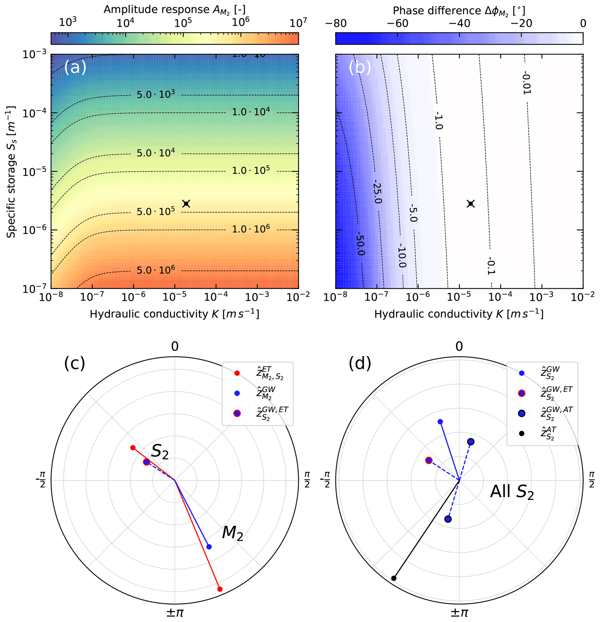
Figure 5 Example amplitude (a) and phase (b) responses calculated for borehole Thirlmere 2 (black dots) using the confined Earth tide model (Sect. 2.2.3). The polar plots show the amplitude and phases of the complex inference of the well response to Earth tides from the response at M₂ (c), and the disentanglement of the well response at atmospheric tide S₂ (d).

The time span and collection frequency of the time series data for the two bores differ. The time series for GW075409.1.2 (Russell, 2012) covers the period from 3 July to 14 December 2018 and was downloaded from the WaterNSW real-time data portal with 15 min intervals. For this bore, coinciding barometric time series data were obtained from a weather station approx. 500 m away. The bore Thirlmere 2 is located about 2 km from GW075409.1.2 and geo-coordinates are shown in Table 2. The time series data for Thirlmere 2 were collected for this study using a vented In-Situ Troll 700H series pressure transducer every 5 min between 23 July and 29 October 2019. The coinciding barometric time series was collected using a Solinst Baro-logger installed in the airspace of the borehole. The field data are summarised in Fig. 4 together with the theoretical ET data for the site.

The borehole GW075409.1.2 at Thirlmere Lakes produced positive M₂ phase shifts (Table 2), with specific storage and hydraulic conductivity therefore being derived from the leaky model (Sect. 2.2.4). Both of the quartz sandstone bores returned Biot–Willis coefficients of 0.96 which requires a value for the grain compressibility (Sect. 2.4.3).

Estimates of hydro-geomechanical parameters – S_s of $\mathrm{3.2}\times {\mathrm{10}}^{-\mathrm{6}}$ and $\mathrm{2.8}\times {\mathrm{10}}^{-\mathrm{6}}$ (1 m⁻¹); k^f of $\mathrm{4.8}\times {\mathrm{10}}^{-\mathrm{7}}$ and $\mathrm{1.9}\times {\mathrm{10}}^{-\mathrm{5}}$ (m s⁻¹) – for the two sandstone bores are considered realistic for a quartz sandstone in this area. The higher k^f for Thirlmere 2 is believed to be indicative of enhanced hydraulic conductivity due to fractures. For this sandstone formation, SCA (2005, 2006) has previously reported S_s values of $\mathrm{2.49}\times {\mathrm{10}}^{-\mathrm{6}}$ to $\mathrm{2.41}\times {\mathrm{10}}^{-\mathrm{4}}$ (1 m⁻¹) and k^f of $\mathrm{1.15}\times {\mathrm{10}}^{-\mathrm{6}}$ to $\mathrm{3.36}\times {\mathrm{10}}^{-\mathrm{6}}$ (m s⁻¹) within this formation, including fracture networks (Ross, 2014). Our estimate of the shear modulus of 2.6 GPa marginally exceeds the expected range of 1–2 GPa (Bertuzzi, 2014; Zhang et al., 2016; Zhang and Lu, 2018). Conversely, the bulk modulus and Young's modulus both fall within the expected ranges of 2.6–5.3 and 3–8 GPa, respectively. The estimated Poisson's ratios of −0.64 and −0.03 are low compared to values between 0.2 and 0.3 typically measured in the laboratory (McMillan et al., 2019).

3.4 Dodowa (Ghana)

Dodowa is located in the Shai Osudoku District in the southeastern part of the Greater Accra Region, Ghana. The local geology consists of the Togo Structural and Dahomeyan Structural units. The Togo is composed of a series of metamorphic and folded quartzites, phyllites, and schists, while the Dahomeyan is composed of altered belts of acid and basic gneisses. BH11 used in this paper is located in a Dahomeyan gneiss (Attoh et al., 1997). All units within the region appear highly weathered, resulting in a 5 m unconsolidated regolith, confining the underlying fractured igneous and metamorphic units.

BH11 was installed and previously studied by Foppen et al. (2020), including AT analysis. The time series for the water levels of BH11 was collected at 20 min intervals between 18 October 2016 and 7 June 2017 using Mini-Diver DI501 (Schlumberger pressure transducers), with atmospheric pressure being recorded with a Mini-Diver DI500 (Schlumberger barometric diver), located above ground (Foppen et al., 2020).

The gneiss bore returned a Biot–Willis coefficient of 0.84, and therefore required a value for the grain compressibility (Sect. 2.4.3).

The hydro-geomechanical estimates of hydraulic conductivity of $\mathrm{2.6}\times {\mathrm{10}}^{-\mathrm{6}}$ (m s⁻¹) and specific storage of $\mathrm{7.2}\times {\mathrm{10}}^{-\mathrm{7}}$ (1 m⁻¹) are comparable with the values for the Togo Structural Unit from Foppen et al. (2020) derived from pumping and slug tests, which indicated ranges of 10⁻⁵–10⁻⁶ (m s⁻¹) and $\mathrm{2.3}\times {\mathrm{10}}^{-\mathrm{7}}$–$\mathrm{7.7}\times {\mathrm{10}}^{-\mathrm{8}}$ (1 m⁻¹), respectively. The estimated porosity of 0.08 for BH11 slightly exceeds the range of 0.005–0.05 in Foppen et al. (2020). Comparison of elastic modulus is problematic for schists, as values are dependent on the original protolith and may vary significantly, and because schistose rock masses are known for high values of anisotropy (Hoek and Diederichs, 2006). For example, Young's modulus for a schist, as in the screened interval of BH11, can vary significantly between 21 and 117 GPa depending on mineralogy and foliation orientation (Condon et al., 2020). Our estimated value of 34.2 GPa falls within this range. However, detailed mineralogy does not exist for this bore to enable a closer comparison with literature values.

3.5 Death Valley (California, USA)

The Death Valley site is located in the western part of the United States on the border of Nevada and California. Bore BLM-1 is located in Paleozoic carbonate rock and was left as an open well. The same time series record was also used in Rau et al. (2020) and it is the same bore for which data were analysed in Cutillo and Bredehoeft (2011). Data were recorded at 15 min intervals using an In-Situ Troll with a vented cable and an In-Situ Barotroll. The time series spans between 25 June and 16 December 2009.

As the Death Valley dataset has previously been analysed by Rau et al. (2020), who justified the use of confined ET, this method was used for the −1^∘ phase shift of the Death Valley dataset which is located in the limit between leaky and confined models.

The estimated hydraulic conductivity of $\mathrm{4.3}\times {\mathrm{10}}^{-\mathrm{6}}$ (m s⁻¹) is in agreement with the ET analysis derived value of $\mathrm{1.3}\times {\mathrm{10}}^{-\mathrm{6}}$ (m s⁻¹) by Cutillo and Bredehoeft (2011). By contrast, the estimated specific storage value of $\mathrm{6.7}\times {\mathrm{10}}^{-\mathrm{7}}$ (1 m⁻¹) is an order of magnitude smaller than the value of $\mathrm{7.3}\times {\mathrm{10}}^{-\mathrm{6}}$ (1 m⁻¹) from Cutillo and Bredehoeft (2011). However, the specific storage and hydraulic conductivity values are both consistent with the values published by Rau et al. (2020) for the same dataset, using a method based on ET. The determined porosity (0.06) also aligns with the lower end of the range proposed by Cutillo and Bredehoeft (2011), and it is reasonable to assume the calculated Young's and shear modulus values of 28.28 and 24.10 GPa are similarly plausible as they compare with literature values (Parent et al., 2015). We note that the derived Poisson's ratio of −0.23 differs significantly from the value of 0.25 which was merely assumed in Cutillo and Bredehoeft (2011).

4 Discussion

4.1 Influences on the quantification of properties

While quantifying hydro-geomechanical properties it is beneficial to consider factors that influence the accuracy of parameter estimation. We note that absolute errors (i.e. offsets) in the measurement of atmospheric or groundwater pressure are irrelevant for the presented methodology. This is because all parameters are based on the amplitude and phase of tidal components embedded within the measurements, i.e. the relative change characteristic of the harmonics. Here, the resolution of the measurement device directly determines detection and quantification of the responses to tidal forces. Schweizer et al. (2021) demonstrated that extraction of harmonics using HALS is accurate if the resolution of the pressure transducer is larger than twice the amplitude of the tidal component under consideration. All instruments deployed in the field examples of this work comfortably fulfilled this criterion. Schweizer et al. (2021) further noted that HALS outperforms the discrete Fourier transform, but also that devising an objective error estimation for HALS is difficult, as it depends on the nature of the residuals (difference between measurement and model), and this requires further investigation. We consider that the accuracy of HALS is at least as good as that resulting from fitting a conceptual model to measurements obtained during standard aquifer testing.

Previous works have illustrated that quantifying BE by disentangling the groundwater response to EAT based on theoretical ET does not lead to additional uncertainty in parameter estimation since it evaluates the relative responses between ET and GW (Acworth et al., 2016). However, this observation is valid only in a subsurface where the hydraulic conductivity is $<K>\mathit{⪆}\mathrm{1}\times {\mathrm{10}}^{-\mathrm{5}}$ m s⁻¹ (Rau et al., 2020). The borehole water level response in lower $<K>$ environments is damped and shifted compared to the pore pressure response outside the bore. A correction requires knowledge of both $<K>$ and S_s, which can be quantified using calculated ET strains. While this has been done before (Hsieh et al., 1987; Xue et al., 2016; Allègre et al., 2016; Rau et al., 2020), there is no literature investigating its associated uncertainties.

4.2 Harmonic disentanglement enables estimation of the poroelastic parameter space

In this work, we make use of recent advances that enable quantitative disentanglement of the groundwater response to both ET and AT forces. Since the two mechanisms act differently on the subsurface, the disentangled responses can be recombined to maximise the outcome. This allows us to solve the complete poroelastic space for unconsolidated systems entirely based on time series of measured groundwater pressure heads, atmospheric pressure, and theoretical ET. For consolidated systems, the complete poroelastic space can also be solved through a system of non-linear equations by assuming a value for grain compressibility, an approach previously used in Rau et al. (2018). While the results in Tables 3 and 4 provide reasonable values, except for Poisson's ratio which is discussed separately below, they are difficult to validate because independent measurements of poroelastic properties are rare.

It is well-established in the literature that a negative phase shift between strain and borehole water levels is representative of confined conditions and only horizontal flow between the formation and the bore (Bower, 1983; Hsieh et al., 1987; Kümpel, 1997; Schulze et al., 2000). Conversely, the meaning of positive phase shifts is not well established in the literature. Although Sect. 2.2.4 is based on the assumption that positive phase shifts relate to a component of vertical flow between the borehole screen and the water table, i.e. semi-confined or leaky conditions (Roeloffs et al., 1989), other explanations for positive phase shifts exist in the literature. These include the influence of fracture transmissivity and length as well as the influence of ocean loading, heterogeneous material properties, and topographic effects (Roeloffs, 1996; Burbey, 2010). Here, positive phases from either vertical flow or fracture flow describe a process in which pressure is able to be propagated rapidly, either to the water table or along a highly transmissive fracture (Bower, 1983). Other mechanisms for phase shifts have also been explored in the broader literature, such as by Hanson and Owen (1982), who related fracture orientation (strike and dip) to either positive or negative phase shifts.

Our results from various field sites show both positive and negative phase shifts. A comprehensive understanding of the causes and interpretation of phase shifts is still lacking in the scientific literature. Shi and Wang (2016) observed that negative phase shifts were indicative of predominantly horizontal groundwater flow in a completely undrained system, while a positive phase shift was indicative of a vertical flow in a semi-confined or unconfined system. The method by Hsieh et al. (1987) outlined above as the confined model (negative phase shift), which was used by Shi and Wang (2016), is based on the assumption of radial horizontal flow into a well. If a positive rather than negative phase shift is used as an input into the system of equations provided by Hsieh et al. (1987), the results will not be sensible. As such, a positive phase shift model is required. For this project the method provided by Wang (2000), and adapted by Xue et al. (2016) and Allègre et al. (2016), was implemented to account for vertical flow. Both Eqs. (13) and (14) were developed for harmonic loading (i.e. ocean or barometric loading) where strain is produced at the Earth's surface and propagated down (Wang and Davis, 1996). ET do not act by surface loading; instead the mechanism is tidal dilatation, where gravitational forces act directly on all mass across the vertical profile. This points to possible issues with simplified conceptual models and the validity of their assumptions. Further research is required to independently validate results derived from passive methods that are based on simplified conceptual understanding and their analytical solutions and to test the influence of different and more complex real-world conditions, such as geological heterogeneity at different scales.

4.3 Strain responses reveal subsurface heterogeneity and anisotropy

Combining ET and AT responses in the subsurface analysis is based on the principle that EAT induce strains with a different directionality. ET are fundamentally cubic, but are approximated as planar (tidal dilatation or strain) (Schulze et al., 2000; Fuentes-Arreazola et al., 2018). However, Rojstaczer and Agnew (1989) stated that the use of the horizontal areal strain from ET is a sufficient approximation for subsurface depths of up to thousands of kilometres, which should cover depths that are relevant to most groundwater systems. For ET, the well water levels must respond to strain in the vicinity of the well bore screen, although the sensitivity to strain that is more distant from the screen is unknown. The subsurface strain response to ET-induced stress depends on the elastic properties, which are highly heterogeneous on a small scale. However, the pore pressure response as measured by a well intersects a larger volume and should therefore be representative of the theoretical values derived from ET calculations.

Rojstaczer and Agnew (1989) predicted that the groundwater response to ET (areal strain) should be high for low porosity and low compressibility. Similarly, for such conditions, the barometric efficiency should approach 1 (BE→1, or equivalently γ→0). However, this is not reflected in our results for Death Valley and Dodowa where the groundwater response magnitude to ET is large but BE is significantly smaller than unity. This phenomenon can be explained by the fact that BE is estimated vertically across a typical geological profile as a surface load, uni-axially compressing the subsurface. Here, consolidation generally increases with depth and we hypothesise that the AT response vertically integrates the material properties above the well screen, i.e. the result is representative of the vertical heterogeneity in elastic properties encountered. The precise geometry of the representative volume from either ET or AT is currently unknown, but it is assumed to be equivalent. However, if this assumption is flawed and the representative volumes of ET or AT significantly differ, strain anisotropy may exist between these two forces and complicate their joint interpretation. Detailed field experimentation or coupled hydraulic-geomechanical modelling would be required to explore these processes.

4.4 Possible reasons for discrepancy in poroelastic properties

Our results in Tables 3 and 4 largely comply with previously established values (Wang, 2000), except for the observation of negative Poisson's ratios. It is important to note that previous studies typically assume a literature value for Poisson's ratio when calculating geomechanical properties (Cutillo and Bredehoeft, 2011). Our new approach based on tidal disentanglement removes the need for such an assumption. However, the negative Poisson's ratios are a surprising result and require explanation. We investigated whether the influence from ocean tide loading could be responsible. However, considering the maximum possible influence from ocean tide loading for each site did not lead to positive Poisson's ratios.

It is theoretically possible for Poisson's ratio to range at $-\mathrm{1}\le \mathit{\nu }\le \mathrm{0.5}$ (Lakes, 1991; Lakes and Witt, 2002). Here, materials with a negative Poisson's ratio are described as auxetic, i.e. materials that become thicker parallel to the direction of the stress. The occurrence of auxetic behaviour in rocks was discussed by Gercek (2007), who summarised that as a Poisson's ratio becomes increasingly negative ($\mathit{\nu }\to -\mathrm{1}$), the material becomes highly resistant to shear deformations but is easy to deform volumetrically. Ji et al. (2018) succinctly describe this relationship for conditions where the shear modulus is much greater than the bulk modulus, defined as $K<\mathrm{2}G/\mathrm{3}$, and geologically is most likely associated with highly anisotropic rocks. This ratio between the bulk and shear modulus is consistent with all results presented in this paper. As such, the negative Poisson's ratios are indicative of the subsurface laterally contracting while being vertically compressed, following the theory of linear poroelasticity.

Negative Poisson's ratios for standard uniaxial core sample testing in thermally induced micro-cracked granites have previously been reported (Homand-Etienne and Houpert, 1989; Zhao et al., 2020). However, auxetic behaviour in rock is predominantly found in studies involving low strains and low confining pressures. For example, in the Berra Sandstone, Handin et al. (1963) observed that small compressive strains (i.e. less than 200 Bar≈2000 m H₂O or 20 MPa) for confining pressure conditions cause the dilatation of pore spaces. Similarly, observations of pore volumes remained constant for moderate strains (20–50 MPa) and reduced in volume for large strains (>50 MPa). Ji et al. (2018) have recently examined auxetic behaviour over a broad range of lithologies and pressures. They concluded that negative Poisson's ratios are possible in crystalline igneous and metamorphic rocks (non-fractured) for confining hydrostatic pressures less than 5 MPa, and less than 200–300 MPa for more quartz-rich sedimentary rocks such as silt stones and sand stones. Further, Ji et al. (2018) observed that the porosity of sedimentary rocks plays an important role in controlling auxetic effects, similar to the nano-scale fabric in artificial auxetic materials (e.g. metallic foams).

The results in this paper are obtained in situ for fully saturated and leaky or confined conditions and caused by small-magnitude strains. Such conditions differ considerably from those used in traditional laboratory techniques for determining elastic moduli (i.e. E, G, K, ν). Compared to the conditions experienced during a compressive laboratory test, or those described above by Ji et al. (2018), the strains caused by EAT are very small. For example, the loading variations caused by the AT component S₂ is typically less than $\mathrm{9}\times {\mathrm{10}}^{-\mathrm{5}}$ MPa (0.1 m H₂O), and the confining pressure caused by an artesian standing water level of 100 m H₂O equates to a confining pressure of only 0.98 MPa. Laboratory results are also well known for demonstrating bias in the sample strength, with the strength decreasing with the sample's increasing physical size. It has been found that this occurs due to the incorporation of more heterogeneity in the sample at larger scales, such as minor lithological changes or discontinuities due to fracturing or jointing (Cundall et al., 2008; Masoumi et al., 2016).

Alternative in situ methods, such as seismic-based methods (Rau et al., 2018), derived positive Poisson's ratios when passing through the same heterogeneous material at the same confining pressures. However, elastic moduli have previously been shown to be frequency dependent when saturated and under confining pressure (Wang, 1993; Tutuncu et al., 1998). Here, we hypothesise that the low frequency of the EAT induced stresses ($\sim \mathrm{2}\mathrm{cpd}\approx \mathrm{2.3}\times {\mathrm{10}}^{-\mathrm{5}}$ Hz), compared to seismic propagated waves (1–100 Hz≈86 400–8 640 000 cpd), causes a highly relaxed response which allows sufficient time for pressure redistribution (Tutuncu et al., 1998). By contrast, the seismic frequency produces a localised un-relaxed or un-drained response as the seismic waves pass through the subsurface, where this effect has been shown to change with the frequency (Pimienta et al., 2016). Both Tutuncu et al. (1998) and Pimienta et al. (2016) provide evidence of decreasing Poisson's ratios with decreasing frequency when below the typical undrained response domain ($<\mathrm{10}\mathrm{Hz}\approx \mathrm{864}\mathrm{000}$ cpd).

For small strains, as relevant for this study, Zaitsev et al. (2017) have shown that the occurrence of negative Poisson's ratios is not as exotic as previously thought. Considering the context of Cundall et al. (2008), Gercek (2007), and Ji et al. (2018), the negative Poisson's ratios derived by TSA in this paper seem plausible. We propose the following possible reasons which could lead to negative Poisson ratio hypotheses for conditions, such as the scale of the effective sample size, anisotropic strain responses from heterogeneities, low confining pressures, the low frequency and small strains caused by EATs, and boundary effects. Meeting the requirements of a negative Poisson's ratio at these small strains is defined by Lakes (1991)as non-affine deformation (non-uniform between scales), non-central forces, and in a state of pre-existing strain (e.g. from overburden). The geomechanical derivations of this paper (Sect. 2.4) are based on linear poroelasticity. However, the auxetic responses observed by Ji et al. (2018) occur both linearly and non-linearly within the negative Poisson's ratio space, depending on the confining pressure and the type of material (Zaitsev et al., 2017). Currently, no relationships between EAT and non-linear poroelastic theory have been established in the literature. Future work in this area should therefore consider the integration of non-linear geomechanics (Khan et al., 1991; Johnson and Rasolofosaon, 1996).

To the best knowledge of the authors, no explicit or robust relationships exist in the literature between elastic moduli results obtained in the field to those estimated from the laboratory testing of core (Leriche, 2017). Similarly, no in situ method currently exists that can derive elastic estimates representative of the large volume of material, such as surrounding a well bore screen, as has been proposed for ET (Zhang et al., 2019). It is likely that heterogeneity within almost any geological media will produce an anisotropic strain response to either ET or AT over such a large volume. Anisotropy may result in apparently atypical properties, e.g. negative Poisson's ratios, and should be investigated for the validity of generic assumptions common to most hydro- or geomechanical investigations of a homogeneous, isotropic aquifer of infinite lateral extent.

4.5 Implications for passive quantification of subsurface hydro-geomechanical properties

There are several uncertainties associated with the findings of this paper, with implications for passive quantification of subsurface hydro-geomechanical properties. These uncertainties and limitations of the method are as follows:

• Although subjective estimates have been attempted (Zhang et al., 2019), the size and scale of the volume of influence from either ET or AT are unknown. It is also possible that there is a difference between the size of influence for ET and AT. Further research is required to elucidate the zone of influence for which the derived properties are representative, such as by numeric modelling.

• Currently the poroelastic response to EAT is considered to be linear. However, rocks have previously been shown to respond in a non-linear manner for undrained, tri-axially loaded laboratory settings, particularly at small strains (Johnson and Rasolofosaon, 1996; Zaitsev et al., 2017). As in situ derivations of rock mass (or sediment) poroelastic values without assuming one or more of the primary values (E, G, K, ν) is relatively novel, the implication of assuming linearity for the analysis of in situ properties remains unknown.

• The mechanism behind leaky responses is believed to be due to a partial drained response in the subsurface. However, the exact causes of such responses are still unknown. In order for the validity of a positive phase shift model to be proven, a more comprehensive understanding of such mechanisms must be further developed.

• Skin and well bore storage effects have been assumed to be negligible in this paper. However, these two effects will alter the phase responses to either ET or AT, as was shown in the recent work by Gao et al. (2020). It is important to note that any phase uncertainties mainly influence the hydraulic conductivity values. However, additional consideration of skin and well bore storage effects will increase the accuracy and confidence in results.

• We note that there is very little literature reporting values let alone ranges of grain compressibility for mineralogy other than quartz, as has been discussed by Rau et al. (2018). Since this is the only real unknown, further work is required to elucidate the effect of grain compressibility uncertainty on the accuracy of the parameter estimation.

Passively characterising the subsurface using the groundwater response to natural signals may improve our understanding of the subsurface. For example, the possibility of auxetic behaviour of subsurface materials in undrained conditions (i.e. hydraulically coupled) will have implications for assessing compaction from groundwater estimates or the stability of slopes and cuttings. Here, the low strain elastic estimates from TSA may provide a lower bounding end-member for plausible ranges of properties. With further study, it may be possible to infer poroelastic properties at different confining pressures and frequencies or to provide a more accurate in situ determination of geomechanical rock properties (e.g. specific storage, strength, etc.) prior to excavation and construction of civil and mining projects. However, further research is required to elucidate the scope of validity (space and time) and transferability of hydro-geomechanical properties derived from different methods.

5 Conclusions

The method developed in this paper provides a comprehensive approach to estimate in situ hydro-geomechanical properties using tidal subsurface analysis (TSA), i.e. from the monitored groundwater response to Earth and atmospheric tides (EAT). Our new method first objectively disentangles the groundwater response to Earth tides (ET) and atmospheric tides (AT) for the dominant response frequencies (M₂ and S₂). Secondly, the approach uses the amplitude and phase responses to ET and AT to determine the complete hydro-geomechanical parameter space: specific storage; hydraulic conductivity; porosity; shear, Young's, and bulk modulus; undrained and drained Poisson's ratio; and Skempton's and Biot–Willis coefficients. Unlike previous research, our new approach does not require an a priori estimate of the Poisson's ratio. However, the application to consolidated systems requires an estimate for the grain compressibility for which literature-based values can be considered if data is unavailable.

Application of our new method to five groundwater and barometric pressure records from four different hydrogeological settings delivers physically realistic results that are consistent with previous estimates. However, we show that the in situ estimates of Poisson's ratio are consistently negative indicating auxetic behaviour. A closer look at the literature reveals that this is not unrealistic and can be attributed to an interplay between simultaneous in situ conditions that differ from those of established laboratory tests. These include a larger effective sample size with scaling effects, anisotropic strain responses due to heterogeneities (e.g. micro-cracking), significantly lower confining pressures, and the small strains at low frequencies caused by the EATs.

Our approach enables the estimation of the complete hydro-geomechanical parameter space in a passive way, i.e. from monitoring records of groundwater pressure head, measured atmospheric pressure, and calculated ET. The primary advantage is that all parameters are determined for the same in situ conditions and that the estimated values therefore should be internally consistent. The new method provides hydro-geomechanical properties of the larger rock mass. This is a clear advantage to methods that require taking samples to the laboratory where replicating field conditions such as in situ confining pressure and representative scale can be problematic. When combined with laboratory estimates on intact rock, it enables evaluation of scale-specific heterogeneity. Further, our method enables more monitoring bores to be tested for hydro-geomechanical properties at a lower cost compared to conventional aquifer pump testing. There is thus the possibility of better characterising the heterogeneity of aquifer properties. However, our method also raises the need for further research in key areas where significant uncertainties remain, e.g. the possibility for non-linearity of the poroelastic response to surface loading and ET forces. Addressing the identified uncertainties could contribute towards improving subsurface monitoring and characterisation in both consolidated and unconsolidated systems.