Analysis of high streamflow extremes in climate change studies: how do we calibrate hydrological models?

Climate change impact studies on hydrological extremes often rely on hydrological models with parameters inferred through calibration procedures using observed meteorological data as input forcing. We show that this procedure can lead to a biased evaluation of the probability distribution of high streamflow extremes when climate models are used. As an alternative approach, we introduce a methodology, coined “Hydrological Calibration of eXtremes” (HyCoX), in which the calibration of the hydrological model, as driven by climate model output, is carried out by maximizing the probability that the modeled and observed high streamflow extremes belong to the same statistical population. The application to the Adige River catchment (southeastern Alps, Italy) by means of HYPERstreamHS, a distributed hydrological model, showed that this procedure preserves statistical coherence and produces reliable quantiles of the annual maximum streamflow to be used in assessment studies.

1 Introduction

The recognition that an altered climate may severely impact water availability and exacerbate floods and droughts has led to a flourish of climate change impact assessment studies over the past decades. Several studies have investigated the likely impact of climate change on hydrology using hydrological modeling performed with meteorological forcing obtained from an ensemble of projections from multiple climate models under different greenhouse gas emission scenarios (e.g., Kundzewicz et al., 2007; Todd et al., 2011; Wilby and Harris, 2006, for a comprehensive review). A wealth of studies have focused on long-term annual and/or seasonal changes in hydrological variables such as runoff, streamflow, snowmelt and soil moisture (e.g., Chiew et al., 2009; Majone et al., 2012; Buytaert and De Bièvre, 2012). Far fewer studies have addressed projected changes in hydrological extremes (i.e., floods and droughts), although they are expected to exert profound and dramatic impacts on agriculture, the economy, human health, energy and many other water-related sectors (e.g., Arnell 2011; Taye et al., 2011; Bouwer, 2013; Thornton et al., 2014).

The role of hydrological calibration and the way to perform it in climate change impact studies has been much debated in the hydrological community (e.g., Peel and Blöschl, 2011; Muñoz et al., 2013; Montanari et al., 2013; Thirel et al., 2014). According to the most commonly used approach, the hydrological model is first calibrated against the observed streamflow using observed meteorological data as input. The calibrated hydrological model is then run with climate models as input to assess the projected changes in selected indicators, including those related to extremes (e.g., flow quantiles; see Ngongondo et al., 2013; Aich et al., 2016; Pechlivanidis et al., 2017; Vetter et al., 2017; Hattermann et al., 2018). The drawbacks of such an approach are, however, twofold: (1) optimality in the reproduction of the time series of observed streamflow does not automatically imply optimality in the reproduction of extremes; and (2) due to epistemic uncertainty, a model calibrated with a given set of observations may respond differently when fed with projections obtained from climate change scenarios. Concerning this latter aspect, some studies have shown that the calibrated model parameters depend on the climatic characteristics of the input forcing used for the calibration of the hydrological model (e.g., Vaze et al., 2010; Laiti et al., 2018). Although recognized, this additional source of uncertainty is mostly ignored in climate change impact studies.

Several studies have suggested that observed streamflow extremes provide valuable information about the hydrological behavior of investigated catchments (Grubbs, 1969; Laio et al., 2010). Similarly, Perrin et al. (2007) and Seibert and Beven (2009) concluded that a limited number of streamflow extremes encapsulate a significant amount of information that may be useful for hydrological model calibration. Beven and Westerberg (2011) also suggested that, when dealing with extremes, including the entire time series might not be informative. This occurs, for instance, when streamflow extremes belong to a different population than ordinary flows (e.g., Calenda et al, 2009), such that the latter does not provide useful information for inferring the former. Hence, quantifying the influence of such extreme events on model calibration is still a challenge in hydrological studies (Brigode et al., 2015) as well as quantifying the uncertainty associated with these estimates (Honti et al., 2014).

To overcome the aforementioned limitations, we propose an innovative methodology in which the calibration of a hydrological model, as driven by climate models, is conducted by maximizing the probability that the modeled and observed streamflow extremes belong to the same population within the reference period. While the approach is exemplified in this work for high streamflows (given the broad interest in the topic), it can be applied to low flows as well (e.g., for drought assessment). The methodology, coined “Hydrological Calibration of eXtremes” (HyCoX), specifically targets climate change impact assessment studies and relies on the use of the two-sample Kolmogorov–Smirnov statistic (Smirnov, 1939) as an efficiency metric during the calibration procedure. We emphasize that the suggested approach is, by definition, a “goal-oriented” framework, as recently discussed in Fiori et al. (2016), Guthke (2017) and Laiti et al. (2018).

Studies adopting the two-sample Kolmogorov–Smirnov test to evaluate whether simulated hydrological variables are distributed according to a given probability distribution (e.g., Kleinen and Petschel-Held, 2007) are relatively common in the literature. This statistical test has also been used to detect changes in hydrological variables (e.g., Wang et al., 2008) as well as to verify if calibrated parameters of a hydrological model belong to a given probability distribution (e.g., Wu et al., 2017; Wang and Solomatine, 2019). This notwithstanding, we are not aware of existing studies adopting this statistical test in the context of hydrological model calibration oriented to the reproduction of extremes.

Therefore, the main objective of the present work is twofold. From one side, we introduce the HyCoX framework and assess its capability to reproduce observed high streamflow extremes using climate models, applied to the same time frame as that of the observational data, as input. On the other, the strength of the proposed methodology is tested against the commonly adopted procedure of calibrating the model using observational data.

The paper is organized as follows: Sect. 2 presents the hydrological modeling framework, the calibration metrics and the adopted statistical test; a description of the study area, the climate change projections, the observational hydrometeorological datasets and the setup of the simulations are summarized in Sect. 3; the main findings are presented and discussed in Sect. 4; and, finally, conclusions are drawn in Sect. 5.

2 Methods

2.1 Hydrological modeling

Hydrological simulations were performed at a daily timescale with the HYPERstreamHS model (Avesani et al., 2021; Laiti et al., 2018; Larsen et al., 2021); HYPERstreamHS couples the HYPERstream routing scheme, recently proposed by Piccolroaz et al. (2016), with a continuous module for surface and subsurface flow generation. The HYPERstream routing scheme is specifically designed to facilitate coupling with climate models and, in general, with gridded climate datasets. HYPERstream can share the same computational grid as that of any overlaying product providing the meteorological forcing while still preserving the geomorphological dispersion of the river network (Rinaldo et al., 1991), irrespective of the grid resolution. This “perfect upscaling” (see Piccolroaz et al., 2016) is obtained via the application of suitable transfer functions derived from a high-resolution digital elevation model (DEM) of the study area. Separation between surface flow and infiltration was obtained using the continuous Soil Conservation Service Curve Number (SCS-CN) model (Michel et al., 2005); this model receives the total precipitation given by the sum of rainfall and snowmelt as input, with the latter being evaluated by the degree-day model coupled with mass balance, which includes snow accumulation (Rango and Martinec, 1995). The infiltrating water enters into a nonlinear bucket mimicking soil moisture dynamics (Majone et al., 2010), with evapotranspiration, which is computed by the Hargreaves and Samani (1982) model, and deep infiltration as output fluxes. Finally, deep infiltration enters a linear bucket used to represent return flow. The surface and subsurface flow generation module has already been successfully applied in previous studies conducted in Alpine catchments (Piccolroaz et al., 2015; Bellin et al., 2016; Galletti et al., 2021). The model requires a total of 12 parameters, which are assumed to be spatially uniform and to be determined through calibration. Spatial heterogeneity of evapotranspiration, infiltration and runoff generation was accounted for by computing all relevant properties for each macrocell (e.g., maximum infiltration capacity, average elevation, soil type and crop coefficient) based on available DEM and land-use/land-cover spatial maps. The list of the 12 parameters, including their units, a short description and the range of variation, is presented in Table 1. A detailed description of the hydrological model can be found in Laiti et al. (2018) and Avesani et al. (2021).

Table 1 List of model parameters with their units and parameter range.

2.2 Hydrological model calibration

The HYPERstreamHS hydrological model was calibrated against streamflow observations using both the ADIGE observational dataset (see Sect. 3.2) and the output of three climate models under two respective emission scenarios as meteorological forcing. A short description of these datasets is provided in Sect. 3.3. Parameters were inferred by optimizing three efficiency metrics using the particle swarm optimization (PSO) algorithm (Kennedy and Eberhart, 1995). PSO is an iterative algorithm belonging to the swarm intelligence category, which is based on the exploration of the space of parameters by a set of particles, called “bees”. Particle's positions were first randomly initialized and then iteratively updated in the search for the optimal solution, with the location-updating procedure considering the memory of all locations visited by the whole collection (swarm) of particles.

The first metric is the classic Nash–Sutcliffe model efficiency (NSE; Nash and Sutcliffe, 1970), which is widely used in hydrological applications:

$$\begin{array}{}\text{(1)}& \mathrm{NSE}=\mathrm{1}-{\displaystyle \frac{{\sum }_{i=\mathrm{1}}^m{\left(Q_{\mathrm{s},i}\left(\mathit{\theta }\right)-Q_{\mathrm{o},i}\right)}^{\mathrm{2}}}{{\sum }_{i=\mathrm{1}}^m{\left(Q_{\mathrm{o},i}-{\overline{Q}}_{\mathrm{o}}\right)}^{\mathrm{2}}}},\end{array}$$

where m is the total number of daily time steps; Q_s,i(θ) and Q_o,i are the simulated (s) and observed (o) streamflow at time step i, respectively; ${\overline{Q}}_{\mathrm{o}}$ is the mean of the observed values; and $\mathit{\theta }=({\mathit{\theta }}_{\mathrm{1}},\mathrm{\dots },{\mathit{\theta }}_q)$ represents the q=12 model parameters. As this metric considers the chronological time series of simulated and observed daily streamflow, it was applied only when the ADIGE observational dataset was used as meteorological input.

The second efficiency metric (R_FDC) is an adaptation of the objective function proposed in Westerberg et al. (2011) to obtain a good match between simulated, ${\widehat{Q}}_{\mathrm{s},\left(i\right)}(\mathit{\theta }$), and observed, ${\widehat{Q}}_{\mathrm{o},\left(i\right)}$, flow duration curves (FDCs; i.e., the ranked streamflow values in descending order):

$$\begin{array}{}\text{(2)}& R_{\mathrm{FDC}}=\mathrm{1}-{\displaystyle \frac{{\sum }_{i=\mathrm{1}}^{n_{\mathrm{EP}}}\left|{\widehat{Q}}_{\mathrm{s},\left(i\right)}^{\mathrm{EP}}\left(\mathit{\theta }\right)-{\widehat{Q}}_{\mathrm{o},\left(i\right)}^{\mathrm{EP}}\right|}{{\sum }_{i=\mathrm{1}}^{n_{\mathrm{EP}}}\left|{\widehat{Q}}_{\mathrm{o},\left(i\right)}^{\mathrm{EP}}-{\overline{Q}}_{\mathrm{o}}\right|}},\end{array}$$

where ${\widehat{Q}}_{\mathrm{s},\left(i\right)}^{\mathrm{EP}}(\mathit{\theta }$) and ${\widehat{Q}}_{\mathrm{o},\left(i\right)}^{\mathrm{EP}}$ are the respective simulated and observed streamflow values at the n_EP evaluation points (EPs) in which the flow duration curves are partitioned, and ${\overline{Q}}_{\mathrm{o}}$ is the mean of the observed time series. According to this metric, R_FDC=1 when the two flow duration curves coincide (i.e., they are the same at all of the EPs). Given that the flow duration curve is insensitive to the chronologic sequence, R_FDC has been used as an objective function for streamflow maxima obtained with both climate models and the ADIGE observational dataset. Furthermore, following Westerberg et al. (2011), the so-called volume method was employed in which EPs were identified as the upper boundary of the elements with the same area $V/n_{\mathrm{EP}}$ below the FDC, where V is the total streamflow volume (i.e., the total area below the FDC). Given the same number of EPs, we remark that the procedure is performed independently for observed and simulated FDCs, and it is indeed possible that the total volume V under the curves and the water volume $V/n_{\mathrm{EP}}$ of the n_EP intervals differ between observations and simulations. The water volume pertaining to each interval and the total water volume of the flow duration curve are computed using the right Riemann sum procedure (Protter and Morrey, 1977). In the computations, we used n_EP=50, which has been shown to obtain the convergence of the numerical integration of Eq. (2) irrespective of the algorithm adopted (Vogel and Fennessey,1994)

The third efficiency metric is the two-sample Kolmogorov–Smirnov (KS) statistic (D_n):

$$\begin{array}{}\text{(3)}& \mathrm{KS}=D_{\mathrm{n}}=\left|F_{\mathrm{s}}\left(Q_{\mathrm{s},\left(i\right)}^M\left(\mathit{\theta }\right)\right)-F_{\mathrm{o}}\left(Q_{\mathrm{o},\left(i\right)}^M\right)\right|,\end{array}$$

where F_s and F_o are the empirical cumulative distribution functions (ECDFs) of the simulated, $Q_{\mathrm{s},\left(i\right)}^M\left(\mathit{\theta }\right)$, and observed, $Q_{\mathrm{o},\left(i\right)}^M$, samples of daily average annual streamflow maxima ranked in increasing order, respectively, and n is the number of years considered in the simulation (29 in the present work, 1 for each year of the investigated period excluding the first 2; see Sect. 3.4). Before ranking the abovementioned streamflow maxima in increasing order, annual streamflow maxima samples are extracted from the chronological daily time series of observed and simulated streamflow, respectively. Following this, ECDFs of the simulated and observed samples of annual maxima are computed according to the classic Weibull formulation (Weibull, 1939):

$$\begin{array}{}\text{(4)}& F_j\left(Q_{j,\left(i\right)}^M\right)={\displaystyle \frac{i}{n+\mathrm{1}}}j=o,s,i\in \left[\mathrm{1},n\right].\end{array}$$

This metric, which is at the core of the proposed approach, aims to maximize the probability that the modeled and observed samples of high streamflow extremes belong to the same population. In other words, among all possible sets of model parameters, we consider the one leading to the smallest maximum absolute distance (D_n) between simulated and observed ECDFs of daily annual streamflow maxima. As KS is not sensitive to the temporal sequence of observed and simulated streamflows, similar to R_FDC, it has been applied to climate projections in addition to the simulations with the ADIGE observational dataset.

2.3 Evaluation of statistical coherence

After calibration, the statistical coherence between the observed and simulated samples of high streamflow extremes was evaluated by employing the two-sample Kolmogorov–Smirnov test (Smirnov, 1939), applied under the null hypothesis that the two samples are drawn from the same underlying distribution. In the two-tail application of interest here, the test statistic D_n is given by Eq. (3). The closer that D_n is to zero, the more likely it is that the two samples are drawn from the same population. In addition, the two-sample Kolmogorov–Smirnov test returns a p value corresponding to the computed D_n statistic (Conover, 1999). The larger the p value, the stronger the evidence in favor of the null hypothesis (i.e., that the samples are drawn from the same distribution).

In this study, the p value has been used as a measure of the statistical coherence between samples of simulated and observed high streamflow extremes. Furthermore, this evaluation step has been performed a posteriori for each simulation experiment described in Sect. 3.4.

2.4 Probability distribution computation and confidence intervals

The theoretical probability distributions of simulated and observed annual streamflow maxima were obtained by fitting an extreme value type I Gumbel distribution (Gumbel, 1941), $P\left(Q\le q\right)=\exp \left[-\exp \left[-\mathit{\beta }\left(q-u\right)\right]\right]$, to the respective samples using the maximum likelihood estimation (MLE) method (Hosking, 1985). The Pearson chi-square test (Pearson, 1990) with a confidence level of α_s=0.05 was then applied to validate the parameters β and u provided by the MLE. Extrapolation of high quantiles (i.e., estimation of quantiles for a return period larger than the available number of observation and simulation years) of observed and simulated annual streamflow maxima was then performed for all of the simulation experiments described in Sect. 3.4.

Confidence intervals of observed streamflow ECDFs were computed using parametric bootstrapping (Efron, 1982) under the assumption that the quantity of interest was distributed according to the abovementioned parametric Gumbel probability distribution. In particular, a 90 % confidence band was estimated using 10 000 uniform random samples from the underlying inferred distribution.

3 Study area, hydroclimatic datasets and the setup of simulations

3.1 Study area

To exemplify the application of the methodology, the upper part of the Adige River basin (Italy), located in the southeastern Alpine region (see Fig. 1), at the Trento gauging station (46^∘04^′13^′′ N, 11^∘06^′54.8^′′ E; drainage area of about 9850 km²) was selected as a case study. The Adige River originates at the Reschen Pass (close to the Alpine divide) and ends its course after 410 km in the northern Adriatic Sea. It is a typical Alpine river basin, with terrain elevations ranging from 185 at Trento to 3500 m a.s.l. at the Italian–Austrian border. The region's morphology is characterized by deep valleys and high mountain crests.

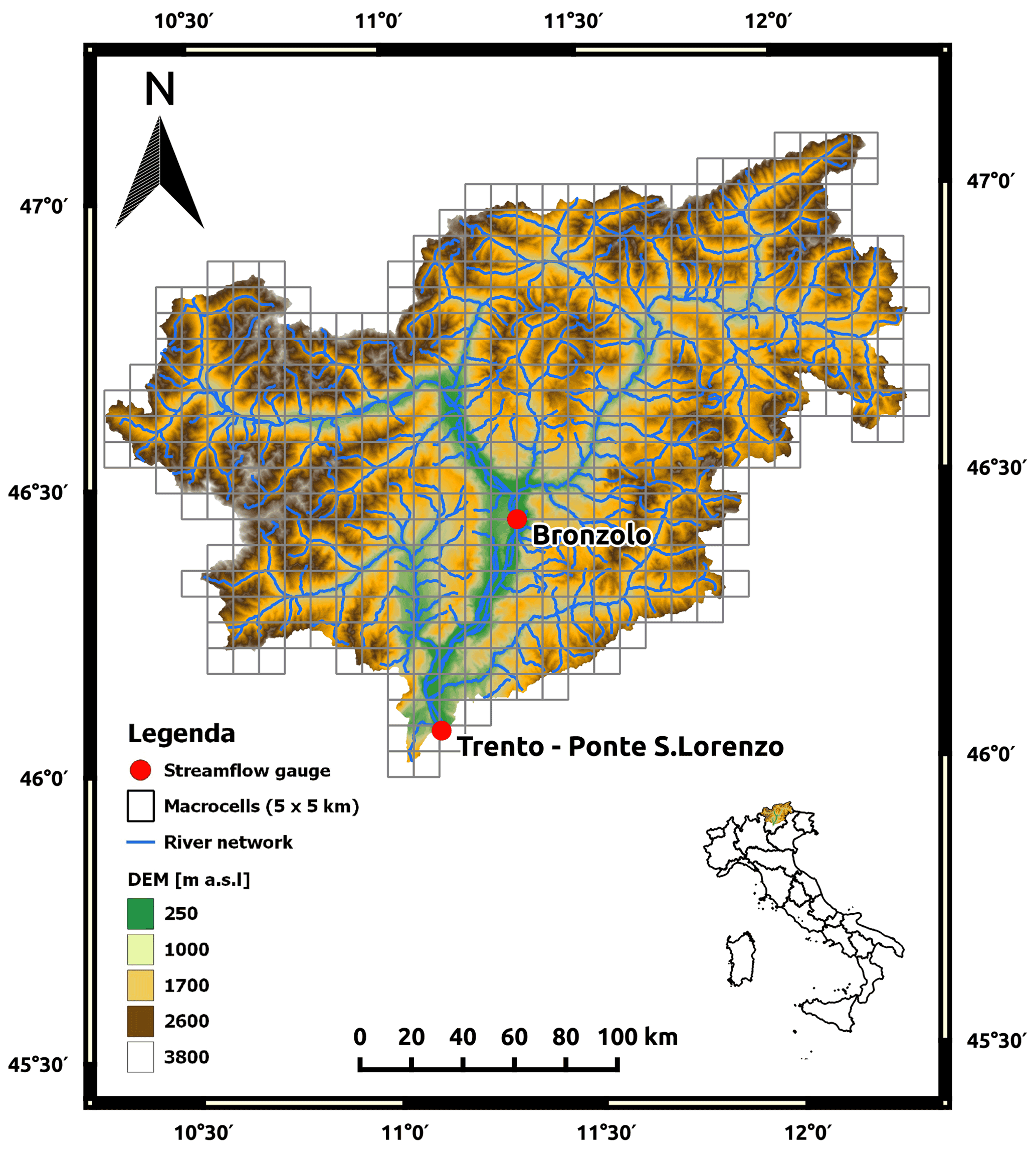
Figure 1 Map of the Adige River basin, with the computational grid cells (“macrocells”) superimposed on the digital elevation model (DEM) and the river network. The streamflow gauging stations used in the study are marked with red dots. The inset shows the location of the Adige River basin within the Italian territory.

The climate of the river basin is characterized by relatively dry and cold winters followed by humid summers and autumns. Streamflow is minimum in winter, when precipitation falls as snow over most of the river basin, and shows two maxima: one occurring early in summer, due to snow melting, and the other in autumn, triggered by intense cyclonic storms. The average annual precipitation ranges from 500 mm in the northwest of the region to 1600 mm in the southern part of the basin (Lutz et al., 2016; Diamantini et al., 2018; Laiti et al., 2018). A projected decrease in snowfall in winter and anticipated earlier snowmelt, essentially due to rising temperatures associated with global warming (Gobiet et al., 2014; Gampe et al., 2016), will likely affect the Adige streamflow regime by the second half of the 21st century (Bard et al., 2015; Majone et al., 2016). This may have relevant consequences on water resources and hydropower production, which is particularly relevant in this region of the Alps (Zolezzi et al., 2009; Bellin et al., 2016; Majone et al., 2016; Avesani et al., 2022); the reader is referred to Chiogna et al. (2016) for a comprehensive review of the hydrological stressors acting in the Adige Basin as well as the area's ecological status.

3.2 Observational datasets

The ADIGE regional dataset, developed by Mallucci et al. (2019) using the meteorological stations within the catchment and in the nearby Austrian territory bounding the catchment from the north, was used as observational precipitation and temperature dataset within the 1950–2010 time window. ADIGE was selected because it is the most accurate gridded meteorological dataset of the investigated river basin (as shown in the recent paper by Laiti et al., 2018). Meteorological data at the selected stations were provided by the Austrian Zentralanstalt für Meteorologie und Geodynamik (https://www.zamg.ac.at/cms/de/aktuell, last access: 15 July 2022) and the meteorological offices of the Autonomous Provinces of Trento (https://www.meteotrentino.it/#!/home, last access: 15 July 2022) and Bolzano (https://weather.provinz.bz.it/Default.asp, last access: 15 July 2022). The time series were interpolated over a 1 km grid at a daily time step using the kriging with external drift algorithm (Goovaerts, 1997; Journel and Rossi, 1989), with an exponential semivariogram using the 16 closest neighboring stations in the linear combination providing the estimate. The optimal spatial distribution model was selected by Mallucci et al. (2019) according to the leave-one-out cross-validation procedure and was applied to both the ordinary kriging and kriging with external drift algorithms. Several semivariogram models (i.e., Gaussian, spherical and exponential models) and different numbers of neighboring stations (namely 8, 16 and 32 stations) were tested, and the model that provided the minimum average absolute error of daily estimates was identified. As described in Mallucci et al. (2019), the optimal semivariogram model was the exponential one, which provided an average absolute error of the daily estimates of about 1.32 mm for precipitation and 0.02 ^∘C for temperature – both comparable with the error estimates provided by widely used datasets available for the Alpine region, such as the Alpine precipitation grid dataset (APGD; Isotta et al., 2014). Daily streamflow at the Ponte San Lorenzo gauging station in Trento and the Bronzolo gauging station (see Fig. 1) were provided by the Hydrological Offices of the Autonomous Province of Trento (https://www.floods.it/public/index.php, last access: 15 July 2022) and Bolzano (https://meteo.provincia.bz.it/default.asp, last access: 15 July 2022), respectively.

3.3 Climate change projections

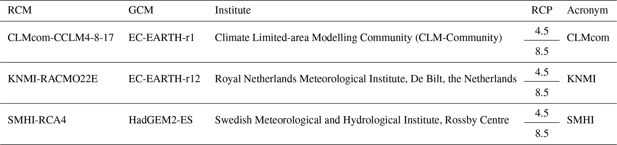
Climate projections used in the present work were derived from the combination of general circulation models (GCMs) and regional climate models (RCMs) available from the EURO-CORDEX initiative under Representative Concentration Pathway (RCP) 4.5 and 8.5 (RCP4.5 and RCP8.5, respectively) at a spatial resolution of about 12 km (EUR-11, https://www.euro-cordex.net/, last access: 15 July 2022, Jacob et al., 2014). To reduce the computational burden of the hydrological modeling experiments, we adopted the model sub-selection proposed by Vrzel et al. (2019), who applied a hierarchical clustering approach (Wilcke and Bärring, 2016) in selected European river basins (including the Adige) to reduce the number of available climate model (CM) simulations (i.e., GCM–RCM combinations) while preserving the variability of the ensemble of climate change signals. In particular, model reduction involved five steps: (1) identification of the meteorological variables; (2) transformation of variables into orthogonal and therewith uncorrelated variables using singular vector decomposition; (3) identification of the optimum number of clusters; (4) hierarchical clustering to group the simulations; and, finally, (5) selection of the simulations closest to the group's mean as representative. This procedure led to the selection of the three GCM–RCM combinations (out of the 12 available), here referred to as CLMcom, KNMI and SMHI (see Table 2).

Table 2 List of the EURO-CORDEX CMs used in this study. The acronyms adopted are listed in the last column.

These three GCM–RCM combinations provide projections of likely future climate changes for the mid-term horizon (2040–2070), with the 1980–2010 time window selected as the period of reference. The projected climate change meteorological signals in the Adige Basin are discussed in Gampe et al. (2016). Both the RCP4.5 and RCP8.5 emission scenarios are available for all of the combinations, thereby leading to a total of six CMs being investigated in the present study (see Table 2). As GCM–RCM combinations are prone to model biases, especially in complex terrain (Kotlarski et al., 2014), bias correction is needed to accurately reproduce historical meteorological forcing during the reference period. In the present work, we rely on products retrieved from EURO-CORDEX; these products are available as bias-corrected values and were corrected with the distribution-based scaling approach (DBS; Yang et al., 2010) using the MESoscale ANalysis system (MESAN) gridded reanalysis datasets of daily precipitation and temperature as observations (Landelius et al., 2016). Basin-averaged monthly mean precipitation and temperature of the six CMs are presented in Fig. 2, with reference to the 1980–2010 period, along with those of the ADIGE dataset. Notice that the CMs differ slightly between the two RCPs as a consequence of (i) the bias correction method adopted, which matches observed and simulated frequency distributions rather than the observations, and (ii) the fact that the correction performed with reference to the 1989–2010 period is extended to the previous 9 years to obtain bias-corrected scenarios for the entire reference period (1980–2010). This is needed because MESAN data are only available for the former period. Figure 2a and b show that basin-averaged monthly mean time series of the six CMs for both variables are in close agreement with ADIGE, with the largest deviations observed in May for precipitation (differences in the range of 15–21 mm) and in December for temperature (differences in the range of 1.3–1.9 ^∘C), respectively. Accordingly, differences at the annual scale are rather small, as highlighted in the insets of Fig. 2a and b. ECDFs of the basin-averaged daily precipitation (Fig. 2c) and temperature (Fig. 2d) for both ADIGE and the six CMs are presented in Fig. 2. For precipitation, no appreciable differences are observed between the CMs and ADIGE throughout the entire range of variability. For the temperature (Fig. 2d), small differences are observed which decrease progressively as temperature increases and become undetectable at high temperatures. Overall, these results indicate that the output of the CMs is in good agreement with the observations during the reference period, a statement which is also valid for the extremes of precipitation and temperature, which are indeed at the base of our approach.

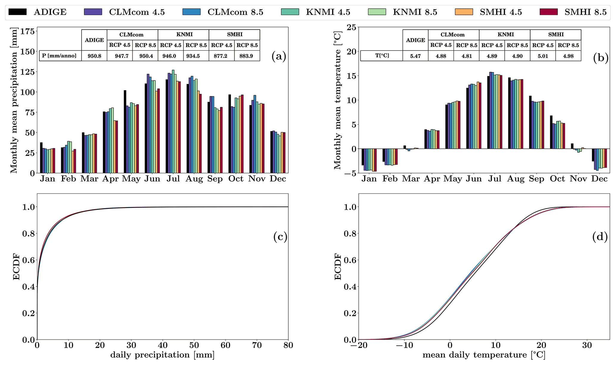
Figure 2 Annual cycle of basin-averaged monthly mean precipitation (a) and temperature (b) during the reference period (1980–2010) for both ADIGE and the six CMs used (different colored bars). The associated annual averages are also shown in the insets. ECDFs of basin-averaged daily precipitation and temperature for the same datasets are presented in subplots (c) and (d), respectively.

3.4 The setup of simulations

All of the simulations were performed with the HYPERstreamHS hydrological model using a daily time step and the 5 km computational grid depicted in Fig. 1. Accordingly, precipitation and temperature provided by the ADIGE dataset and by the six CM simulations presented in Sect. 3.3 were projected onto this grid using the nearest-neighbor method. Notice that the contributing area of the macrocells at the border of the domain was reduced by the amount belonging to the neighboring basin, so as to preserve the overall contributing area of the investigated case study.

In a first set of simulations presented in Sect. 4.1, the HYPERstreamHS model was calibrated at the Trento gauging station using the NSE, KS and R_FDC metrics as objective functions and the 1980–2010 period as a reference. In order to ease the presentation of results, these three parameterizations are hereafter called NSE-ADIGE, KS-ADIGE and R_FDC-ADIGE, respectively. Validation of the modeling framework was then performed for these three parameterizations by computing the efficiency metrics at the Bronzolo gauging station (drainage area of about 6000 km²; see Fig. 1) within the same time window as well as at the Trento gauging station in the 1950–1980 period (which was not used for calibration).

In a second set of simulations (presented in Sect. 4.2), we assessed whether the model calibrated with observational data and fed with precipitation and temperature obtained from climate models produced samples of annual streamflow maxima that were statistically coherent with the observations. Here, we considered simulations performed in the 1980–2010 period using precipitation and temperature from the three GCM–RCM combinations, selected as described in Sect. 3.3, for both respective RCP4.5 and RCP8.5 emission scenarios and for a total of six CM combinations (see Table 2). The parameters of the hydrological model were those referring to the NSE-ADIGE, KS-ADIGE and R_FDC-ADIGE parameterizations.

In Sect. 4.3, we present the results of the calibration experiments performed using the precipitation and temperature distributions provided by the six CMs for the 1980–2010 period in HYPERstreamHS with KS and R_FDC as objective functions. Following the procedure described in Sect. 2.4, extrapolations were then performed under the assumption that simulated and observed ECDFs were distributed according to the parametric Gumbel probability distribution. The Pearson chi-square test was then applied to verify the inferred model.

For all time windows and all simulations, the first 2 years were used as spin-up and were, therefore, excluded from the computation of model performance. Furthermore, statistical coherence between simulated and observed samples of annual streamflow maxima was evaluated a posteriori using the p values associated with the Kolmogorov–Smirnov two-sample test described in Sect. 2.3.

The effects of calibrations conducted using different meteorological forcing (observational data and CMs simulations) on model parameters are investigated in Sect. 4.4 with reference to the KS metric. For each calibration experiment performed with the PSO algorithm, we considered 100 particles that, with a maximum number of 400 iterations, lead to a maximum of 40 000 hydrological simulations for each external forcing. The parameter ranges considered during the search for the optimal solution are presented in Table 1, and they have been set by means of preliminary simulations so as to minimize the probability of excluding combinations of parameters which lead to behavioral solutions (Beven and Binley, 1992). In addition, as a metric of uncertainty for the calibrated parameter, we considered the range, $\overline{d}$, between the maximum and minimum value of each parameter in the 200 simulations presenting the highest efficiency metric (see Piccolroaz et al., 2015). We remark that the procedure adopted here aims to only to quantify the differences in the range of calibrated parameters and not to perform a full uncertainty analysis of predictions.

Finally, in Sect. 4.5 the projected changes in high flow extremes in the future period from 2040 to 2070 are evaluated. For each CM, we considered the following parameterizations obtained during calibration in the reference period: (1) calibrations with KS and R_FDC as objective functions and (2) NSE-ADIGE as representative of a standard calibration procedure using the observational dataset ADIGE as input forcing.

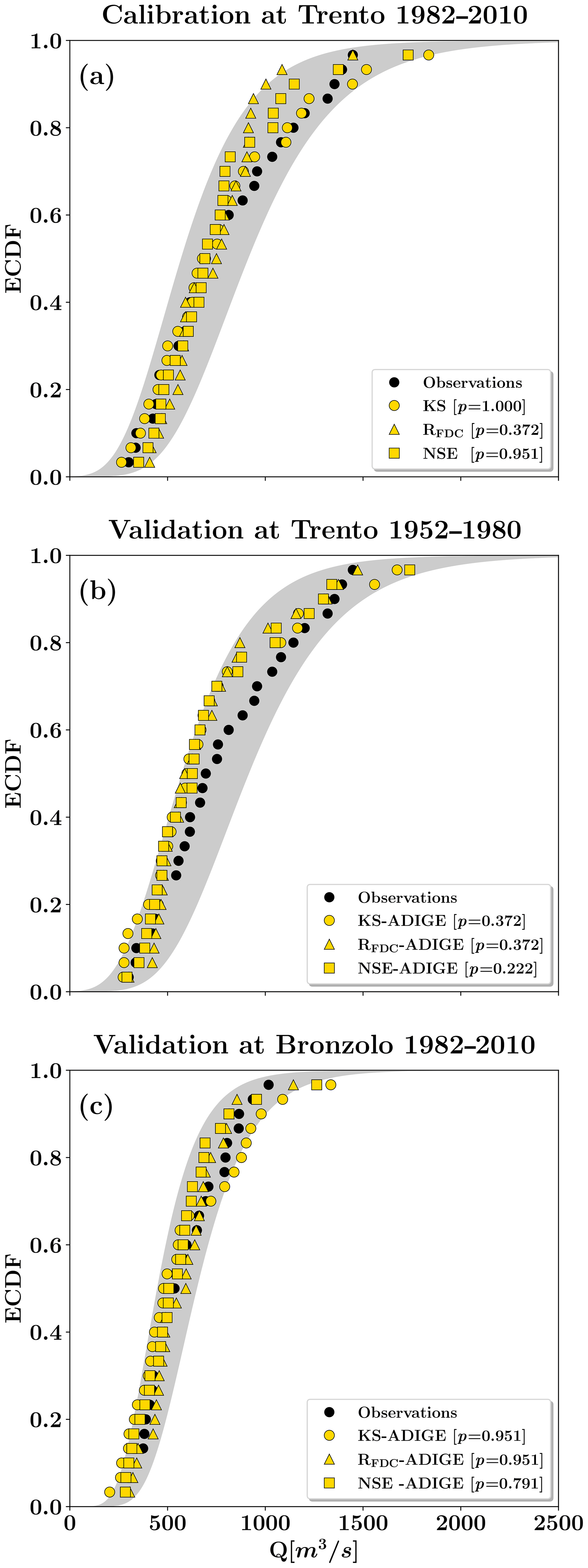
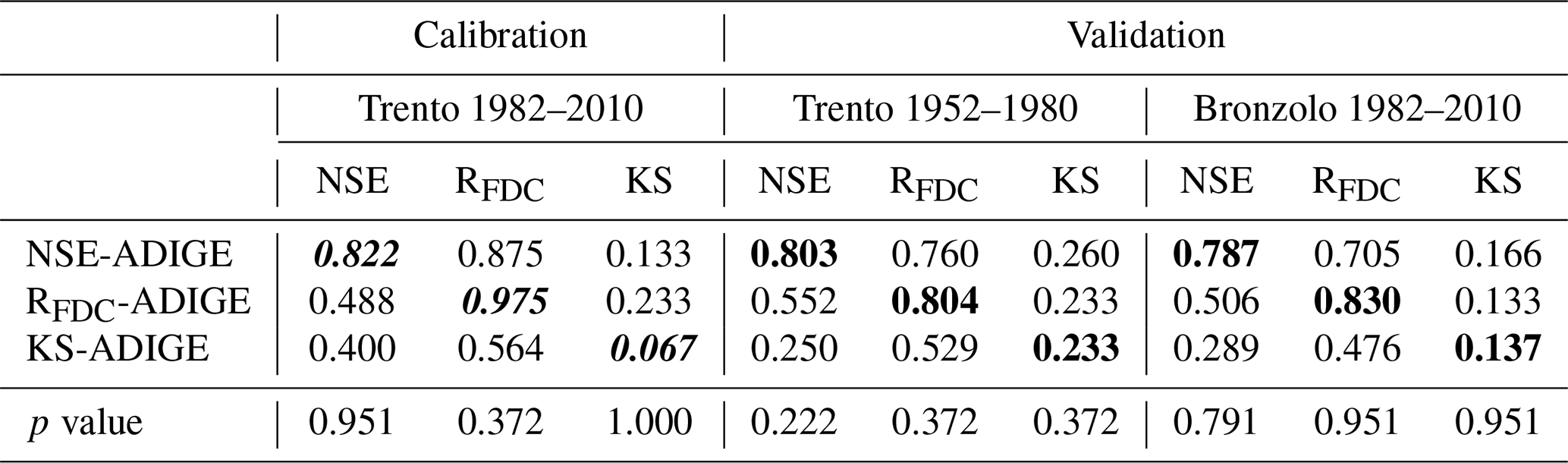
Figure 3 ECDFs of the daily annual streamflow maximum obtained using the observational dataset ADIGE and the NSE-ADIGE, KS-ADIGE and R_FDC-ADIGE parametrizations at (a) the Trento gauging station during the 1982–2010 period, (b) the Trento gauging station during the 1952–1980 period and (c) the Bronzolo gauging station during the 1982–2010 period as input. The experimental ECDFs obtained from streamflow observations during the same time frames are shown using black bullets, and the gray shaded area indicates the associated 90 % confidence interval of the fitted Gumbel distribution. The p values of the Kolmogorov–Smirnov two-sample test are also reported in brackets for each simulation run.

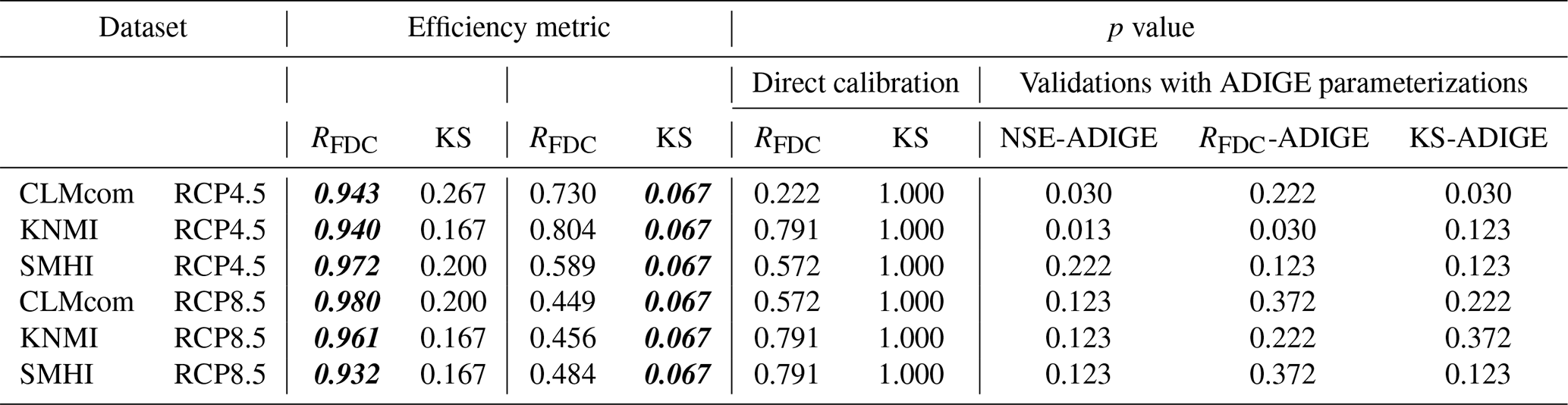
Table 3 Efficiency metrics for calibration and validation runs obtained using the ADIGE dataset as input forcing. The terms NSE-ADIGE, KS-ADIGE and R_FDC-ADIGE refer to the parameterizations described in Sect. 3.4. Bold italic numbers indicate the metric optimized in the calibration. The p values of the Kolmogorov–Smirnov (KS) test are also reported (bottom line) for the calibration experiments and the validation runs highlighted by bold numbers.

4 Results and discussion

4.1 Simulations using the ADIGE observational dataset

Figure 3a shows the simulated ECDFs obtained using the three metrics, NSE, KS and R_FDC, as objective functions and the ADIGE observational dataset as input forcing. Table 3 shows the associated p values of the Kolmogorov–Smirnov test. From a statistical viewpoint, all three metrics provide simulated samples of annual streamflow maxima belonging to the same population as the observed ones, given that p>0.05 in all cases, with a maximum for KS (p=1.000) and a minimum for R_FDC (p=0.372). However, calibration conducted using KS as an objective function leads to NSE and R_FDC values (0.4 and 0.564, respectively; see Table 3) that are lower than those obtained when calibration is performed by (separately) optimizing these two metrics (NSE=0.822 and R_FDC=0.975, respectively; see Table 3). This is in accordance with several studies showing that the adoption of a given metric in calibration may lead to suboptimal results for other metrics because each of them is sensitive to specific aspects of the time series with its limitations and trade-offs (see, e.g., Schaefli and Gupta, 2007; Gupta et al., 2009; Mcmillan et al., 2017; Fenicia et al., 2018). This latter limitation is, in our opinion, outweighed by the improvements in representing the ECDFs of observed high flow extremes when the model is calibrated explicitly considering such information, i.e., by minimizing the KS metric. Accordingly, in our analyses, the use of different efficiency metrics leads to different simulated ECDFs and, hence, to different p values in the application of the statistical coherence test (see Table 3).

Validation of the hydrological modeling framework was performed by evaluating the model performance in the time frame from 1952 to 1980, which was not used for calibration, at the Ponte San Lorenzo gauging station in Trento. The validation was done using the ADIGE dataset as input and the parameterizations obtained by calibrating the model in the 1982–2010 time frame (i.e., NSE-ADIGE, R_FDC-ADIGE and KS-ADIGE, as described above). The NSE-ADIGE and R_FDC-ADIGE parameterizations led to NSE and R_FDC values that were only slightly lower than those obtained in calibration (NSE=0.803 and R_FDC=0.804; see Table 3). The KS-ADIGE parameterization led to an increase in the KS from 0.067 during calibration to 0.233 during validation, which was still rather small. The limited modification of the efficiency metrics during validation is an encouraging result which shows that the HYPERstreamHS model provides a good representation of the hydrological system independent of the metric adopted during calibration. The simulated and observed ECDFs of annual streamflow maxima and the associated p value of the Kolmogorov–Smirnov test are presented in Fig. 3b. Reproduction of the observed ECDF is satisfactorily for all three parameterizations, particularly for high flow quantiles, with p values in the range between 0.222 and 0.372 (see also Table 3). The three parameterizations provide simulated samples of annual streamflow maxima belonging to the same population of observations (also in the time window from 1952 to 1980); the reduction in the p value from calibration to validation is significant but rather common in hydrological models.

Spatial validation of the modeling framework was also performed by simulating streamflow at the Bronzolo gauging station (see Fig. 1) during the same time window as the calibration conducted at the Trento gauging station (1982–2010). Similarly to the previous case, efficiency metrics during validation evidence a small reduction in performance with respect to those obtained during calibration (see Table 3). On the other hand, the results presented in Fig. 3c highlight an excellent reproduction of the observed ECDF of annual streamflow maxima for all three parameterizations, with the associated p values in the range between 0.791 (NSE-ADIGE) and 0.951 (R_FDC-ADIGE and KS-ADIGE). The latter is a noteworthy result which indicates that the parameterization obtained using KS as an objective function is reliable, although relying on a limited number of observations, and does not introduce distortion in the spatial representation of the hydrological processes, particularly those controlling high streamflow events (i.e., runoff generation and streamflow concentration processes). This latter aspect will be further investigated in Sect. 4.4.

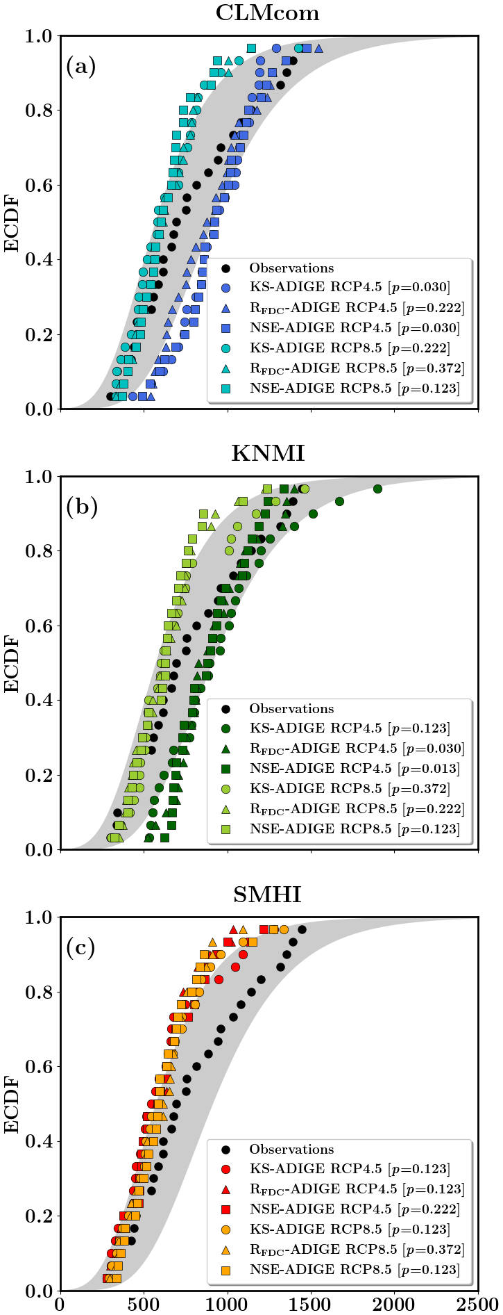
Figure 4 ECDFs of the annual maximum streamflow at the Trento gauging station during the 1982–2010 period obtained using the NSE-ADIGE, KS-ADIGE and R_FDC-ADIGE parameterizations and the (a) CLMcom, (b) KNMI and (c) SMHI climate models as input forcing for both the RCP4.5 and RCP8.5 emission scenarios. The experimental ECDF is shown with black dots, and the gray shaded area indicates the associated 90 % confidence interval of the fitted Gumbel distribution. The p values of the Kolmogorov–Smirnov two-sample test are also reported in brackets for each simulation run.

Table 4 The R_FDC and KS efficiency metrics for the 1982–2010 period with forcing provided by the CLMcom, KNMI and SMHI climate models under the respective RCP4.5 and RCP8.5 emission scenarios. Bold italic numbers indicate the metric optimized in the calibration. The p values of the Kolmogorov–Smirnov (KS) test are also reported for all of the calibration experiments and for the validations conducted using the NSE-ADIGE, KS-ADIGE and R_FDC-ADIGE parametrizations.

4.2 Simulations using parameterizations derived from calibrations with observed ground data

Here, we analyze the case in which HYPERstreamHS was run in the time frame from 1982 to 2010 using the meteorological variables produced by the climate models and the three parameterizations, NSE-ADIGE, R_FDC-ADIGE, KS-ADIGE (described in Sect. 3.4), as input. Visual inspection of Fig. 4a, b and c shows that, for high quantiles, the simulated ECDFs are often outside the 90 % confidence interval of the Gumbel distribution fitted to observations for all of the considered combinations of CMs and parameterizations. The p values of these validation runs are shown in the last three columns of Table 4. In particular, these three parameterizations lead to p values that are always lower than p=0.372 for all of the considered CMs and emission scenarios (see Table 4). NSE-ADIGE and R_FDC-ADIGE show the lowest p values on average, with KS-ADIGE performing slightly better: p=0.372 for KNMI and SMHI under the RCP8.5 scenario (see Fig. 4b and c and Table 4). Inspection of Table 4 also reveals that values of p<0.05, and thus simulated ECDFs not belonging to the same population as the measured one, are obtained with the CLMcom model for both the NSE-ADIGE and KS-ADIGE parameterizations under both emission scenarios as well as with the KNMI model for the NSE-ADIGE and R_FDC-ADIGE parameterizations under RCP4.5.

The above results highlight how classic approaches based on feeding hydrological models, calibrated using observed meteorological data and employing customary efficiency metrics (i.e., NSE and R_FDC), with meteorological forcing provided by climate models produce results characterized by low statistical coherence with the observational data. Furthermore, our results indicate that the same drawback arises when employing parameterizations obtained with a calibration approach optimizing the desired statistic of extremes but still using observational data as input (i.e., KS-ADIGE in Fig. 4a, b and c). These results are in agreement with previous studies evidencing that the hydrological models, calibrated against observed data, that perform well within a baseline period may not be accurate nor consistent for simulating streamflow under future climate conditions (Brigode et al., 2013; Lespinas et al., 2014). Indeed, it is recognized that the use of different datasets can lead to different optimized parameters that will partially account for their specific climate characteristics (Yapo et al. 1996; Vaze et al., 2010; Laiti et al., 2018). Furthermore, it is acknowledged that climate change impact simulations are affected by uncertainty in climate modeling, but the calibration strategy adopted during the reference period also plays a role (Lespinas et al., 2014; Mizukami et al., 2019). In this respect, we showed that the statistical coherence between climate scenarios and observations (i.e., high streamflow extremes in our case) should be preserved during hydrological calibration, at least in the reference period. This latter aspect will be further discussed in the ensuing Sect. 4.3.

4.3 Performance of the hydrological model calibrated using climate model outputs as input

Table 4 summarizes the efficiency metrics and the p values of the calibration experiments performed using the precipitation and temperature distributions provided by the six selected CMs with KS and R_FDC as the objective functions in HYPERstreamHS. Simulations refer to the 1982–2010 period. When KS was used in calibration, all six simulations provided samples of annual streamflow maxima that had a high probability (i.e., p=1.000, column 8 of Table 4) of belonging to the same population of observed values. A similar conclusion was reached for the objective function R_FDC but with lower p values (column 7 of Table 4), although these values were larger than p=0.05 – the level of significance customarily adopted in the statistical literature to reject the null hypothesis. The lowest p value was obtained with the CLMcom climate model under the RCP4.5 emission scenario with R_FDC as the objective function (p=0.222; see column 7 of Table 4). Consistently, the absolute maximum distances between the ECDFs of observed and simulated samples obtained using R_FDC as the calibration metric are always larger than those obtained using KS (see the third and fifth columns in Table 4). When calibration is performed with KS, the results are satisfactorily with respect to the R_FDC metric, which is in the range between 0.449 and 0.804 for all of the CMs (see the fourth column in Table 4). As R_FDC employs the entire time series of observational data, this result evidences the fact that using the KS metric in calibration does not introduce model overparameterization, despite the reduced number of observational data used (i.e., 29 values of observed daily annual streamflow maxima).

The appreciable difference between the observed and simulated ECDFs obtained in the calibration experiments conducted using the KS and R_FDC metrics is highlighted in Fig. 5. Figure 5 shows that the ECDFs obtained by extracting the annual maxima from the simulations calibrated with KS as the objective function are in a better agreement with the observed ECDFs than those obtained by calibrating with R_FDC. This comparison highlights that the KS metric is preferable to R_FDC when dealing with high flow extremes, thereby strengthening the approach envisaged here of directly addressing the desired statistics of extremes in calibration instead of calibrating the hydrological model on the entire streamflow record.

Figure 5 Simulated ECDFs of the daily annual maximum streamflow at the Trento gauging station during the 1982–2010 period with precipitation and air temperature provided by the CLMcom (a, b), KNMI (c, d) and SMHI (e, f) climate models under the respective RCP4.5 (a, c, e) and RCP8.5 (b, d, f) emission scenarios. Calibration of HYPERstreamHS was performed using both the KS and R_FDC metrics as objective functions. The ECDF of observations is shown with black dots, and the gray shaded area indicates the associated 90 % confidence interval of the fitted Gumbel distribution. The p values of the Kolmogorov–Smirnov two-sample test are also reported in brackets for each simulation run.

The literature reports a few examples of hydrological models calibrated using tailored information instead of the entire observed streamflow time series (e.g., Montanari and Toth, 2007; Blazkova and Beven, 2009; Westerberg et al., 2011; Lindenschmidt, 2017). However, these approaches are typically adopted for reproducing the basin response to observed meteorological forcing and have not been applied (to our best knowledge) in combination with GCM–RCM simulations in climate change impact studies. The only example somewhat similar to our approach that we found in the literature is that of Honti et al. (2014), who used a stochastic weather generator trained by observed weather time series coupled with observed discharge data to sample the posterior distribution of model parameters. The adoption of a time-independent calibration, for which time shift does not influence the objective function, has the intrinsic advantage of allowing the use of GCM–RCM runs conducted without the assimilation of observational data, as in our case. In fact, these runs provide time-slice experiments representing a stationary climate for both reference and future periods (see, e.g., Majone et al., 2012) and, by definition, cannot be used in the context of a classic day-by-day hydrological comparison experiment with observed historical data (see, e.g., Eden et al., 2014).

Quantiles of daily annual streamflow maxima as a function of the return period at the Trento gauging station are shown in Fig. 6, where the results obtained by calibrating the hydrological model with the meteorological input provided by the climate models (with the KS and R_FDC metrics as objective functions) are compared with those obtained using the same meteorological input but employing the NSE-ADIGE, R_FDC-ADIGE and KS-ADIGE parameterizations. Visual inspection of Fig. 6 reveals that, for all return periods, parameterizations obtained by calibrating with the observed precipitation and temperature data, as provided by the ADIGE dataset, significantly underestimate the quantiles of the observations and fall outside the confidence interval of the fitted Gumbel distribution (i.e., outside the gray area). The only exceptions are the quantiles derived from simulations conducted with the KNMI (KS-ADIGE; dotted line in Fig. 6c) and CLMcom (all three metrics; Fig. 6a) climate models under the RCP4.5 emission scenario. We note, however, that these curves are obtained with forward simulations, providing low KS p values with respect to the other cases (always lower than p=0.222). Instead, quantiles obtained from simulations optimized directly using climate models and with KS as the metric are in a very good agreement with the experimental data, whereas those obtained using R_FDC are outside or at the lower bound of the interval of confidence, although they are generally in a better agreement with the quantiles of the experimental data than those obtained with the aforementioned NSE-ADIGE, R_FDC-ADIGE and KS-ADIGE parametrizations. Exceptions to this are the quantiles obtained with CLMcom and KNMI under the RCP4.5 emission scenario with R_FDC as the metric, which are characterized by the largest deviations from observations (see Fig. 6a and c, respectively). We attribute this occurrence to the additional source of uncertainty arising from the extrapolation procedure (i.e., the selection of the probability distribution and of the statistical inference method for the parameters, MLE in our case). The confidence interval of the fitted Gumbel distribution to the observational data (gray area) widens as the return period increases; this is in line with the recent findings of Meresa and Romanowicz (2017), who showed that errors in fitting theoretical distribution models to annual maxima streamflow series might contribute significantly to the overall uncertainty associated with projections of future hydrological extremes.

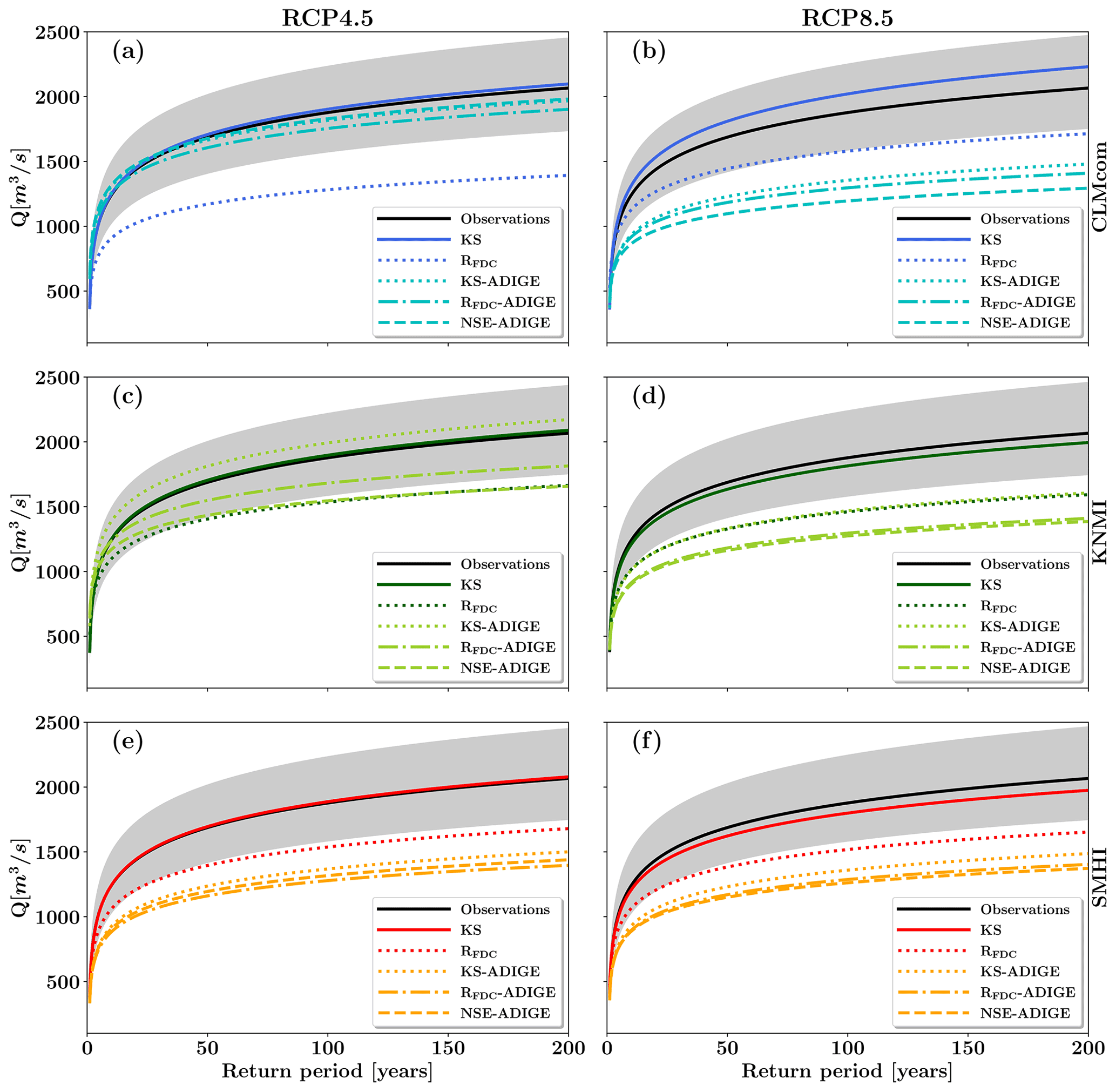
Figure 6 Quantiles of the daily annual streamflow maxima as a function of return period at the Trento gauging station. Extrapolations are based on simulations conducted during the 1982–2010 period using the CLMcom (a, b), KNMI (c, d) and SMHI (e, f) climate models as input forcing under the respective RCP4.5 (a, c, e) and RCP8.5 (b, d, f) emission scenarios. Each curve represents a combination of CM, emission scenario and parameterization obtained with the calibration. Simulations conducted with the parameterizations obtained using the ADIGE observational dataset for calibration are labeled as follows: NSE-ADIGE, R_FDC-ADIGE and KS-ADIGE. Extrapolation from observed streamflow maxima is also shown (continuous black line), and the gray shaded area indicates the associated 90 % confidence interval of the fitted Gumbel distribution.

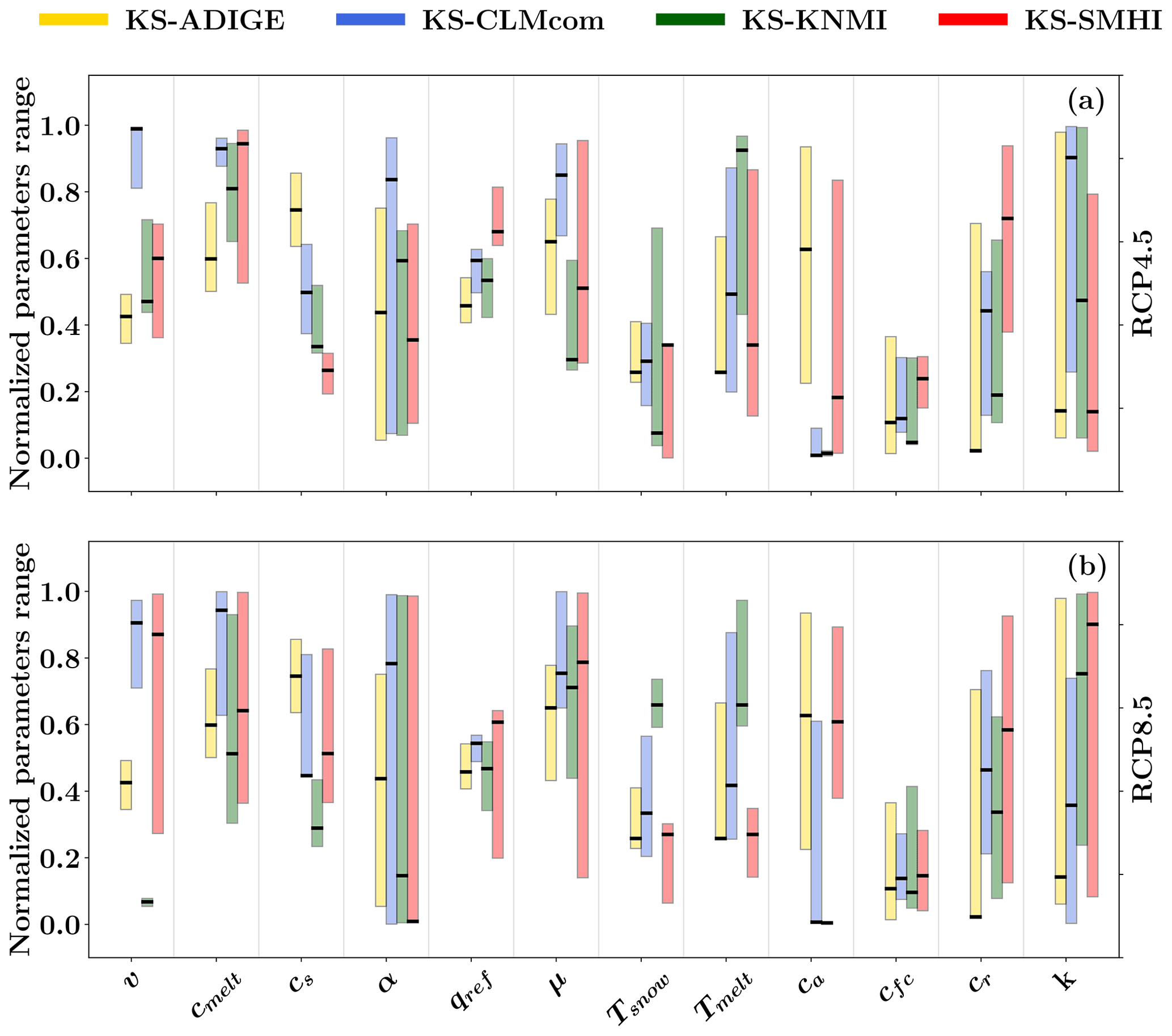
Figure 7 The range ($\overline{d}$) between the maximum and minimum value of each parameter associated with the 200 simulations presenting the highest efficiency plotted as a normalized range with respect to the parameter range presented in Table 1. Calibrations are conducted for the three different CMs under the respective (a) RCP4.5 and (b) RCP8.5 emission scenarios with reference to the KS metric. Bold horizontal segments indicate the optimal parameter sets for all experiments.

4.4 Model parameters

The results presented in the previous sections highlight that better statistical coherence between observations and simulations (performed with CM simulations as input) was achieved by optimizing the desired statistics of extremes, in our case KS (see the curves labeled KS in Figs. 5 and 6), in the calibration of the hydrological model. Starting from this evidence, we investigated the effect (on the model parameters) of performing the calibration using either observed data or meteorological data derived from CMs with KS as the objective function. Figure 7 shows the range ($\overline{d}$) between the maximum and minimum values, which is represented here by the length of the vertical bar of each parameter among the 200 accepted values corresponding to the behavioral models (see Sect. 3.4), and the corresponding optimal parameter set, which is represented by a horizontal segment. The values of the parameters are normalized with respect to their range (see Table 1) such that they are directly comparable. In all simulations the normalized parameter range $\overline{d}$ is well distributed between zero and one, indicating a proper choice of the parameter range in the PSO algorithm, although the optimal value was located close to the boundary of the search domain for a few parameters. As shown in Fig. 7 the majority of the parameters obtained using the proposed approach span a range ($\overline{d}$) that is similar to (or slightly larger than), in terms of amplitude, that obtained for KS-ADIGE, thereby supporting the conclusion that calibration using CM simulations does not lead (for either RCP) to bias parameterizations. Figure 7 also shows that, for most of the parameters, simulations performed with CMs lead to generally overlapping ranges for $\overline{d}$ with respect to the case in which the ADIGE observational dataset was used. The largest deviations in terms of $\overline{d}$ are observed for KS-KNMI, particularly under the RCP8.5 emission scenario. Notably, the parameters shaping the continuous soil moisture accounting module result in values of the optimum which are very similar for all cases (see q_ref, μ and c_fc in Fig. 7a and b). Visual inspection of Fig. 7 also highlights that the parameters controlling runoff generation and streamflow concentration (in particular, v, c_s, q_ref and c_fc) present very good identifiability (i.e., a small range, $\overline{d}$). This is not the case for parameters controlling snow melting and groundwater contribution, with the latter being relevant only for low flow conditions (see k in Fig. 7a and b). These results, as well as the good performance obtained in the validation runs presented in Sect. 4.1, suggest that, although the model is calibrated considering a limited number of observations, the maxima are well reproduced in the continuous simulations, but this is achieved only if the interaction between the precipitation and streamflow relevant during high flow extremes is correctly reproduced. We cannot exclude that additional analyses could be envisioned for improving the identifiability of some parameters (e.g., by reducing the number of model parameters or introducing constraints in the parameter's range) in applications dealing with different hydrological models and different data availabilities (e.g., lower number of streamflow extremes). However, the analysis presented here provides clear evidence that the parameterizations derived from the use of the KS metric are reliable.

The differences observed in the optimal values of model parameters are due to the use of meteorological forcing datasets with different capabilities to reproduce the present climate. Along with the concepts brought forward here, this source of uncertainty can be addressed effectively via calibration of the hydrological model to the quantities of interest (i.e., the observed streamflow statistics of extremes) using the forcing provided by a specific CM as input. This approach can be seen as a “hydrologically based bias correction” and is rooted in the adoption of a goal-oriented calibration framework (see, e.g., Laiti et al., 2018), as stated in the Sect. 1.

4.5 Projected changes in streamflow quantiles

Figure 8 shows the annual maximum streamflow at the Trento gauging station as a function of the return period in the future time window (2040–2070) and for the six selected CMs. Visual inspection of Fig. 8 confirms that, in all cases, using the standard calibration (i.e., NSE-ADIGE) of the hydrological model leads to a significant underestimation of all quantiles with respect to using KS and R_FDC. This is in agreement with the results obtained for the reference period (see Fig. 6), where simulations using the NSE-ADIGE parameterization provided streamflow quantiles systematically lower than those obtained with the CMs. In addition, KS-based calibrations always provide larger quantiles with respect to the cases in which the R_FDC metric is adopted (considering the same RCP emission scenario). We note that the adoption of the KS metric is preferable, as it provided an almost perfect match with observed streamflow quantiles in the calibration period (see Fig. 6).

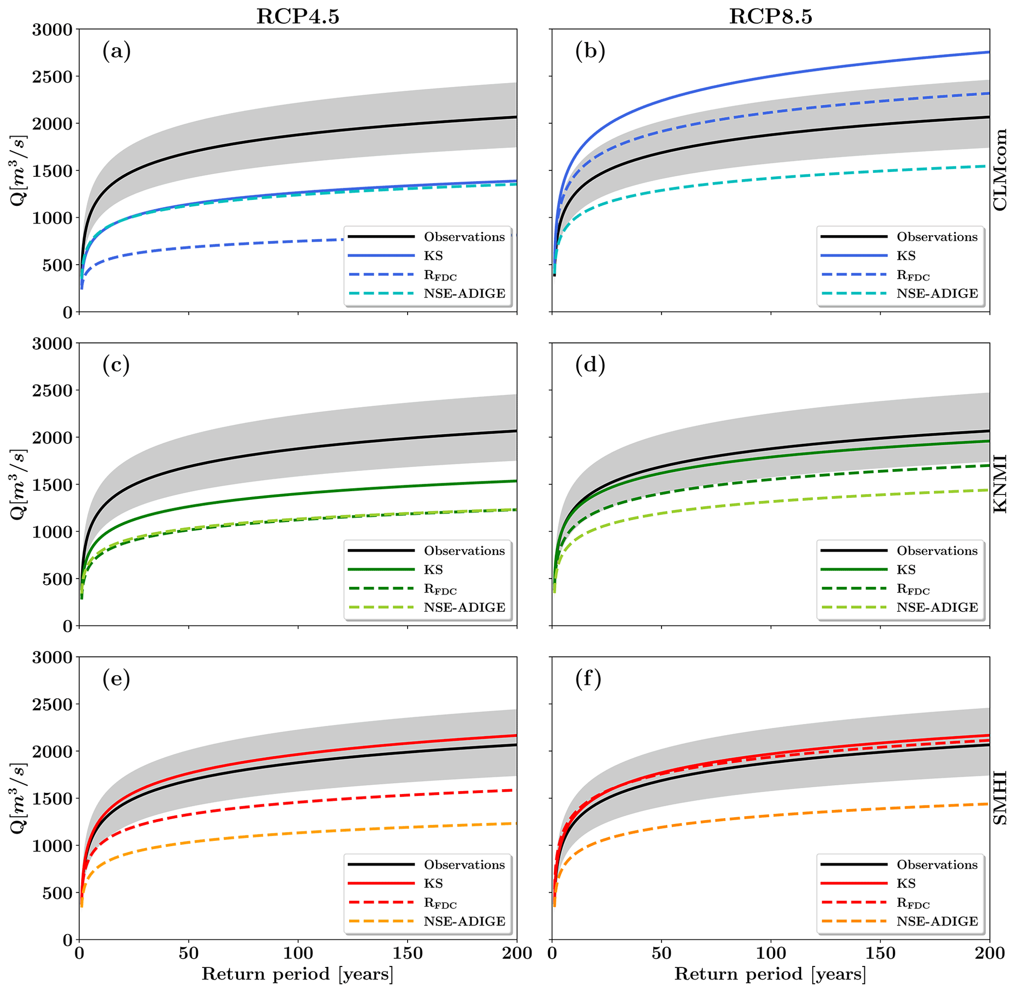
Figure 8 Quantiles of the annual maximum daily streamflow as a function of return period at the Trento gauging station. Projections are based on simulations of the future time period from 2042 to 2070 using the CLMcom (a, b), KNMI (c, d) and SMHI (e, f) climate models under the respective RCP4.5 (a, c, e) and RCP8.5 (b, d, f) emission scenarios as input. The continuous black line shows the quantile distribution of high flow extremes evaluated with the observational data of the 1982–2010 period, and the gray shaded area indicates the associated 90 % confidence interval of the fitted Gumbel distribution.

Moreover, Fig. 8 shows that projected changes in high flows extremes depend on the selected CM and emission scenario. Projected streamflow quantiles under RCP8.5 are larger than those under RCP4.5 for all of the CMs. In general, the projected streamflow quantiles do not exceed those obtained by fitting the Gumbel distribution to the observational data of the 1982–2010 period (continuous black lines in Figs. 6 and 8), with the exceptions of the CLMcom and SMHI models under the RCP8.5 emission scenario and SMHI under the RCP4.5 emission scenario when the KS metric is adopted. These results are in line with other recent contributions which concluded that the sign and magnitude of projected changes in high flow extremes will vary significantly with the location of the investigated river basin, the climate models used, the emission scenario and the selection of the time window (Ngongondo et al., 2013; Aich et al., 2016; Pechlivanidis et al., 2017; Vetter at al., 2017). Our results are in line with the analysis of Brunner et al. (2019), who implemented a stochastic framework to simulate future streamflow time series in 19 regions of Switzerland and concluded that future maximum streamflow will increase and decrease in rainfall-dominated and snowmelt-dominated regions, respectively. Similarly, Di Sante et al. (2019) showed that a moderate increase in high flow magnitude (return time of 100 years) is projected for large river basins (drained area >10 000 km²) in the central Europe region under the RCP8.5 scenario and considering a mid-century time slice.

5 Conclusions

In this work, we proposed the HyCoX methodological framework in which the calibration of the hydrological model is carried out by maximizing the probability that the modeled and observed high streamflow extremes belong to the same statistical population. The proposed framework is goal-oriented and aims at improving the estimation of streamflow extremes by directly calibrating the selected hydrological model to the quantities of interest (i.e., flow statistics instead of time series) using the meteorological data provided by climate models as input. In particular, the framework relies on the use of the two-sample Kolmogorov–Smirnov (KS) statistic as the objective function during the calibration procedure. This approach ensures statistical coherence between scenarios and observations in the reference period, and it likely preserves statistical coherence in the future climate change scenario runs performed to project changes in streamflow extremes. The goal-oriented approach envisaged in this work can be applied to a variety of hydrological scenarios and modeling approaches. Furthermore, we remark that the HyCoX methodology is not a metric-dependent approach, and any type of metric assessing the statistical coherence between observed and simulated streamflow extremes can be employed without any loss of generality.

The proposed procedure is exemplified via the application of six climate models and observational data to the analysis of the annual maximum streamflow of the Adige River basin (Italy) using the HYPERstreamHS distributed hydrological model. While the approach is exemplified here for high flows, it can be applied to low flows as well (e.g., for drought assessment). The results highlight that adopting the KS is preferable to other popular metrics (e.g., the NSE or fit to flow duration curve, R_FDC) when dealing with high streamflow extremes. This validates our hypothesis that directly addressing the statistics of the extremes under consideration during the calibration exercise leads to coherent and reliable hydrological models for assessing the impact of climate change. We warn that such an approach may lead to suboptimal performance if the target is different from the one employed in this study, which is in line with the goal-oriented framework pursued here. Alternatively, a multi-objective approach could be envisioned to investigate the trade-off in model performance emerging from the use of multiple metrics, including the one proposed here. This latter aspect is indeed beyond the objective of the present contribution, although it is worthy of further analysis. Furthermore, the investigation of optimal values highlighted that direct calibration using CM outputs and KS as the objective function leads to unbiased identification of model parameters.

Overall, we showed that the way in which the hydrological model is calibrated against observations assumes paramount importance in climate change impact assessments on streamflow extremes. In particular, we highlighted how the classic approach of calibrating using daily streamflow observations with observed meteorological data can lead to a biased probability distribution of streamflow extremes when climate models are used as input forcing during the reference period, with high streamflow quantiles being dramatically underestimated with respect to the fitted distribution of the observed extremes. Extrapolations performed using the proposed calibration procedure, with input provided by CMs, are instead more reliable, and they provide a good match with observed quantiles.