Deep learning rainfall–runoff predictions of extreme events

The most accurate rainfall–runoff predictions are currently based on deep learning. There is a concern among hydrologists that the predictive accuracy of data-driven models based on deep learning may not be reliable in extrapolation or for predicting extreme events. This study tests that hypothesis using long short-term memory (LSTM) networks and an LSTM variant that is architecturally constrained to conserve mass. The LSTM network (and the mass-conserving LSTM variant) remained relatively accurate in predicting extreme (high-return-period) events compared with both a conceptual model (the Sacramento Model) and a process-based model (the US National Water Model), even when extreme events were not included in the training period. Adding mass balance constraints to the data-driven model (LSTM) reduced model skill during extreme events.

1 Introduction

Deep learning (DL) provides the most accurate rainfall–runoff simulations available from the hydrological sciences community (Kratzert et al., 2019b, a). This type of finding is not new – Todini (2007) noted more than a decade ago, in his review of the history of hydrological modeling, that “physical process-oriented modellers have no confidence in the capabilities of data-driven models’ outputs with their heavy dependence on training sets, while the more system engineering-oriented modellers claim that data-driven models produce better forecasts than complex physically-based models.” Echoing this sentiment about the perceived predictive reliability of data-driven models, Sellars (2018) reported in their summary of a workshop on “Big Data and the Earth Sciences” that “[m]any participants who have worked in modeling physical-based systems continue to raise caution about the lack of physical understanding of ML methods that rely on data-driven approaches.”.

The idea that the predictive accuracy of hydrological models based on physical understanding might be more reliable than machine learning (ML) based models in out-of-sample conditions was drawn from early experiments on shallow neural networks (e.g., Cameron et al., 2002; Gaume and Gosset, 2003). However, although this idea is still frequently cited (e.g., the quotations above; Herath et al., 2020; Reichstein et al., 2019; Rasp et al., 2018), it has not been tested in the context of modern DL models, which are able to generalize complex hydrological relationships across space and time (Nearing et al., 2020b). Further, there is some evidence that this hypothesis might not be true. For example, Kratzert et al. (2019a) showed that DL can generalize to ungauged basins with better overall skill than calibrated conceptual models in gauged basins. Kratzert et al. (2019b) used a slightly modified version of a long short-term memory (LSTM) network to show how a model learns to transfer information between basins. Similarly, Nearing et al. (2019) showed how an LSTM-based model learns dynamic basin similarity under changing climate: when the climate in a particular basin shifts (e.g., becomes wetter or drier), the model learns to adapt hydrological behavior based on different climatological neighbors. Further, because DL is currently the state of the art for rainfall–runoff prediction, it is important to understand its potential limits.

The primary objective of this study is to test the hypothesis that data-driven models lose predictive accuracy in extreme events more than models based on process understanding. We focus specifically on high-return-period (low-probability) streamflow events and compare four models: a standard deep learning model, a physics-informed deep learning model, a conceptual rainfall–runoff model, and a process-based hydrological model.

2 Methods

2.1 Data

The hydrological sciences community lacks community-wide standardized procedures for model benchmarking, which severely limits the effectiveness of new model development and deployment efforts (Nearing et al., 2020b). In previous studies, we used open community data sets and consistent training/test procedures that allow for results to be directly comparable between studies; we continue that practice here to the extent possible.

Specifically, we used the Catchment Attributes and Meteorology for Large-sample Studies (CAMELS) data set curated by the US National Center for Atmospheric Research (NCAR) (Newman et al., 2015; Addor et al., 2017a). The CAMELS data set consists of daily meteorological and discharge data from 671 catchments in the contiguous United States (CONUS), ranging in size from 4 to 25 000 km², that have largely natural flows and long streamflow gauge records (1980–2008). We used 498 of the 671 CAMELS catchments; these catchments were included in the basins that were used for model benchmarking by Newman et al. (2017), who removed basins (i) with large discrepancies between different methods of calculating catchment area and (ii) with areas larger than 2000 km².

CAMELS includes daily discharge data from the United States Geological Survey (USGS) National Water Information System (NWIS), which are used as training and evaluation target data. CAMELS also includes several daily meteorological forcing data sets (Daymet; the North American Land Data Assimilation System, NLDAS, data set; and Maurer). We used NLDAS for this project because we benchmarked against the National Oceanic and Atmospheric Administration (NOAA) National Water Model (NWM) CONUS Retrospective Dataset (NWM-Rv2, introduced in detail in 2.3.2), which also uses NLDAS. CAMELS also includes several static catchment attributes related to soils, climate, vegetation, topography, and geology (Addor et al., 2017a) that are used as input features. We used the same input features (meteorological forcings and static catchment attributes) that were listed in Table 1 by Kratzert et al. (2019b).

2.2 Return period calculations

The return periods of peak annual flows provide a basis for categorizing target data in a hydrologically meaningful way. This results in a metric that is consistent while maintaining diversity across basins – e.g., a similar flow volume may be “extreme” in one basin but not in another. Splitting model training and test periods by different return periods allows us to assess model performance on both rare and effectively unobserved events.

For return period calculations, we followed guidelines in the U.S. Interagency Committee on Water Data Bulletin 17b (IACWD, 1982). The procedure is to fit all available annual peak flows (log transformed) for each basin to a Pearson type III distribution using the method of moments:

$$\begin{array}{}\text{(1)}& f(y;\mathit{\tau },\mathit{\alpha },\mathit{\beta })={\displaystyle \frac{\left(\frac{y-\mathit{\tau }}{\mathit{\beta }}{)}^{\mathit{\alpha }-\mathrm{1}}\exp \right(-\frac{y-\mathit{\tau }}{\mathit{\beta }})}{\left|\mathit{\beta }\right|\mathrm{\Gamma }\left(\mathit{\alpha }\right)}},\end{array}$$

with $\frac{y-\mathit{\tau }}{\mathit{\beta }}>\mathrm{0}$ and distribution parameters τ, α, and β, where τ is the location parameter, α is the shape parameter, β is the scale parameter, and Γ(α) is the gamma function.

To calculate the return periods, we used annual peak flow observations taken directly from the USGS NWIS, instead of from the CAMELS data, as the Bulletin 17b guidelines require annual peak flows, whereas CAMELS provides only daily averaged flows. The Bulletin 17b (IACWD, 1982) guidelines require the use of all available data, which range from 26 to 116 years for peak flows. After fitting the return period distributions for each basin, we classified each water year of the CAMELS data from each basin (each basin-year of data) according to the return period of its observed peak annual discharge.

This return period analysis does not account for nonstationarity – i.e., the return period of a given magnitude of event in a given basin could change due to changing climate or changing land use. There is currently no agreed upon method to account for nonstationarity when determining flood flow frequencies, so it would be difficult to incorporate this in our return period calculations. However, for the purpose of this paper (testing whether the predictive accuracy of the LSTM is reliable in extreme events), this is not an issue because stationary return period calculations directly test predictability on large events that are out of sample relative to the training period, which for practical purposes can represent potential nonstationarity.

2.3 Models

2.3.1 ML models and training

We test two ML models: a pure LSTM and a physics-informed LSTM that is architecturally constrained to conserve mass – we call this a mass-conserving LSTM (MC-LSTM; Hoedt et al., 2021). These models are described in detail in Appendices A and B.

Daily meteorological forcing data and static catchment attributes data were used as inputs features for the LSTM and MC-LSTM, and daily streamflow records were used as training targets with a normalized squared-error loss function that does not depend on basin-specific mean discharge (i.e., large and/or wet basins are not overweighted in the loss function):

$$\begin{array}{}\text{(2)}& \mathrm{NSE}*={\displaystyle \frac{\mathrm{1}}{B}}\sum _{b=\mathrm{1}}^B\sum _{n=\mathrm{1}}^N{\displaystyle \frac{({\widehat{y}}_n-y_n{)}^{\mathrm{2}}}{\left(s\right(b)+\mathit{ϵ}{)}^{\mathrm{2}}}},\end{array}$$

where B is the number of basins, N is the number of samples (days) per basin B, ${\widehat{y}}_n$ is the prediction for sample n ($\mathrm{1}\le n\le N$), y_n is the corresponding observation, and s(b) is the standard deviation of the discharge in basin b ($\mathrm{1}\le b\le B$), calculated from the training period (see Kratzert et al., 2019b).

We trained both the standard LSTM and the MC-LSTM using the same training and test procedures outlined by Kratzert et al. (2019b). Both models were trained for 30 epochs using sequence-to-one prediction to allow for randomized, small minibatches. We used a minibatch size of 256, and, due to sequence-to-one training, each minibatch contained (randomly selected) samples from multiple basins. The standard LSTM had 128 cell states and a 365 d sequence length. Input and target features for the standard LSTM were pre-normalized by removing bias and scaling by variance. For the MC-LSTM, the inputs were split between auxiliary inputs, which were pre-normalized, and the mass input (in our case precipitation), which was not pre-normalized. Gradients were clipped to a global norm (per minibatch) of 1. Heteroscedastic noise was added to training targets (resampled at each minibatch) with a standard deviation of 0.005 times the value of each target datum. We used an Adam optimizer with a fixed learning rate schedule; the initial learning rate of 1×10³ was decreased to 5×10⁴ after 10 epochs and 1×10⁴ after 25 epochs. Biases of the LSTM forget gate were initialized to 3 so that gradient signals persisted through the sequence from early epochs.

The MC-LSTM used the same hyperparameters as the LSTM except that it used only 64 cell states, which was found to perform better for this model (see Hoedt et al., 2021). Note that the memory states in an MC-LSTM are fundamentally different than those of the LSTM due to the fact that they are physical states with physical units instead of purely information states.

All ML models were trained on data from the CAMELS catchments simultaneously. We used three different training and test periods:

1. The first training/test period split was the same split used in previous studies (Kratzert et al., 2019b, 2021; Hoedt et al., 2021). In this case, the training period included 9 water years, from October 1 1999 through September 30 2008, and the test period included 10 water years, from 1990 to 1999 (i.e., from 1 October 1989 through 30 September 1999). This training/test split was used only to ensure that the models trained here achieved similar performance compared to previous studies.

2. The second training/test period split used a test period that aligns with the availability of benchmark data from the US National Water Model (see Sect. 2.3.2). The training period included water years 1981–1995, and the test period included water years 1996–2014 (i.e., from 1 October 1995 through 30 September 2014). This was the same training period used by Newman et al. (2017) and Kratzert et al. (2019a) but with an extended test period. This training/test split was used because the NWM-Rv2 data record is not long enough to accommodate the training/test split used by previous studies (item above in this list).

3. The third training/test period split used all water years in the CAMELS data set with a 5-year or lower return period peak flow for training, whereas the test period included water years with greater than a 5-year return period peak flow in the period from 1996 to 2014 (to be comparable with the test period in the item above). This is to test whether the data-driven models can extrapolate to extreme events that are not included in the training data. Return period calculations are described in Sect. 2.2. To account for the 365 d sequence length for sequence-to-one prediction, we separated all training and test years in each basin by at least 1 year (i.e., we removed years with high return periods as well as their preceding years from the training set). A file containing the training/test year splits for each CAMELS basin based on return periods is available in the GitHub repository linked in the “Code and data accessibility” statement.

Nash and Sutcliffe (1970)Gupta et al. (2009)Gupta et al. (2009)Gupta et al. (2009)Yilmaz et al. (2008)Yilmaz et al. (2008)Yilmaz et al. (2008)Kratzert et al. (2021)

Table 1 Overview of evaluation metrics. The notation of the original publications is kept.

2.3.2 Benchmark models and calibration

The conceptual model that we used as a benchmark was the Sacramento Soil Moisture Accounting (SAC-SMA) model with SNOW-17 and a unit hydrograph routing function. This same model was used by Newman et al. (2017) to provide standardized model benchmarking data as part of the CAMELS data set; however we recalibrated SAC-SMA to be consistent with our training/test splits that are based on return periods. We used the Python-based SAC-SMA code and calibration package developed by Nearing et al. (2020a), which uses the SPOTPY calibration library (Houska et al., 2019). SAC-SMA was calibrated separately at each of the 531 CAMELS basins using the three training/test splits outlined in Sect. 2.3.1.

The process-based model that we used as a benchmark was the NOAA National Water Model CONUS Retrospective Dataset version 2.0 (NWM-Rv2). The NWM is based on WRF-Hydro (Salas et al., 2018), which is a process-based model that includes Noah-MP (Niu et al., 2011) as a land surface component, kinematic wave overland flow, and Muskingum–Cunge channel routing. NWM-Rv2 was previously used as a benchmark for LSTM simulations in CAMELS by Kratzert et al. (2019a), Gauch et al. (2021), and Frame et al. (2021). Public data from NWM-Rv2 are hourly and CONUS-wide – we pulled hourly flow estimates from the USGS gauges in the CAMELS data set and averaged these hourly data to daily over the time period from 1 October 1980 through 30 September 2014. As a point of comparison, Gauch et al. (2021) compared hourly and daily LSTM predictions against NWM-Rv2 and found that NWM-Rv2 was significantly more accurate at the daily timescale than at the hourly timescale, whereas the LSTM did not lose accuracy at the hourly timescale vs. the daily timescale. All experiments in the present study were done at the daily timescale.

NWM-Rv2 was calibrated by NOAA personnel on about 1400 basins with NLDAS forcing data on water years 2009–2013. Part of our experiment and analysis includes data-driven models trained on irregular years, specifically with water years that include a peak flow annual return period of less than 5 years, and the calibration of the conceptual model (SAC-SMA) was also done on these years. Without the ability to recalibrate NWM-Rv2 on the same time period as the LSTM, MC-LSTM, and SAC-SMA, we cannot directly compare the performance of NWM-Rv2 with the other models. This model still provides a useful benchmark for the data-driven models, even if it does have a slight advantage over the other models due to the calibration procedure.

2.3.3 Performance metrics and assessment

We used the same set of performance metrics that were used in previous CAMELS studies (Kratzert et al., 2019b, a, 2021; Gauch et al., 2021; Klotz et al., 2021). A full list of these metrics is given in Table 1. Each of the metrics was calculated for each basin separately on the whole test period for each of the training/test splits described in Sect. 2.3.1 except for the return-period-based training/test split. In the former case (contiguous training/test periods), our objective is to maintain continuity with previous studies that report statistics calculated over entire test periods. In the latter case (return-period-based training/test splits), our objective is to report statistics separately for different return periods; therefore, it is necessary to calculate separate metrics for each water year and each basin in the test period. The last metric outlined in Table 1, the absolute percent bias of peak flow only for the largest streamflow event in each water year, lets us assess the ability to extrapolate to high-flow events. The metric was calculated separately for each annual peak flow event in all three training/test splits.

3 Results

3.1 Benchmarking whole hydrographs

Table 2 provides performance metrics for all models (Sect. 2.3.2) on the three test periods (Sect. 2.3.1). Appendix C provides a breakdown of the metrics in Table 2 by annual return period.

Table 2 Median performance metrics across 498 basins for two separate time split test periods and a test period split by the return period (or probability) of the annual peak flow event (i.e., testing across years with a peak annual event above a 5-year return period, or a 20 % probability of annual exceedance).

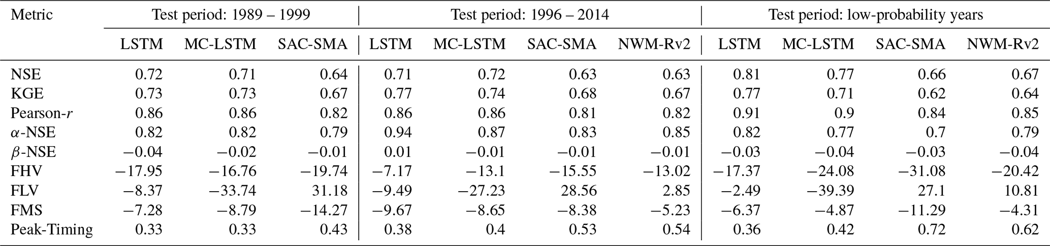
The first test period (1989–1999) is the same period used by previous studies, which allows us to confirm that the DL-based models (LSTM and MC-LSTM) trained for this project perform as expected relative to prior work. The performance of these models (according to the metrics) is broadly equivalent to that reported for single models (not ensembles) by Kratzert et al. (2019b) (LSTM) and Hoedt et al. (2021) (MC-LSTM).

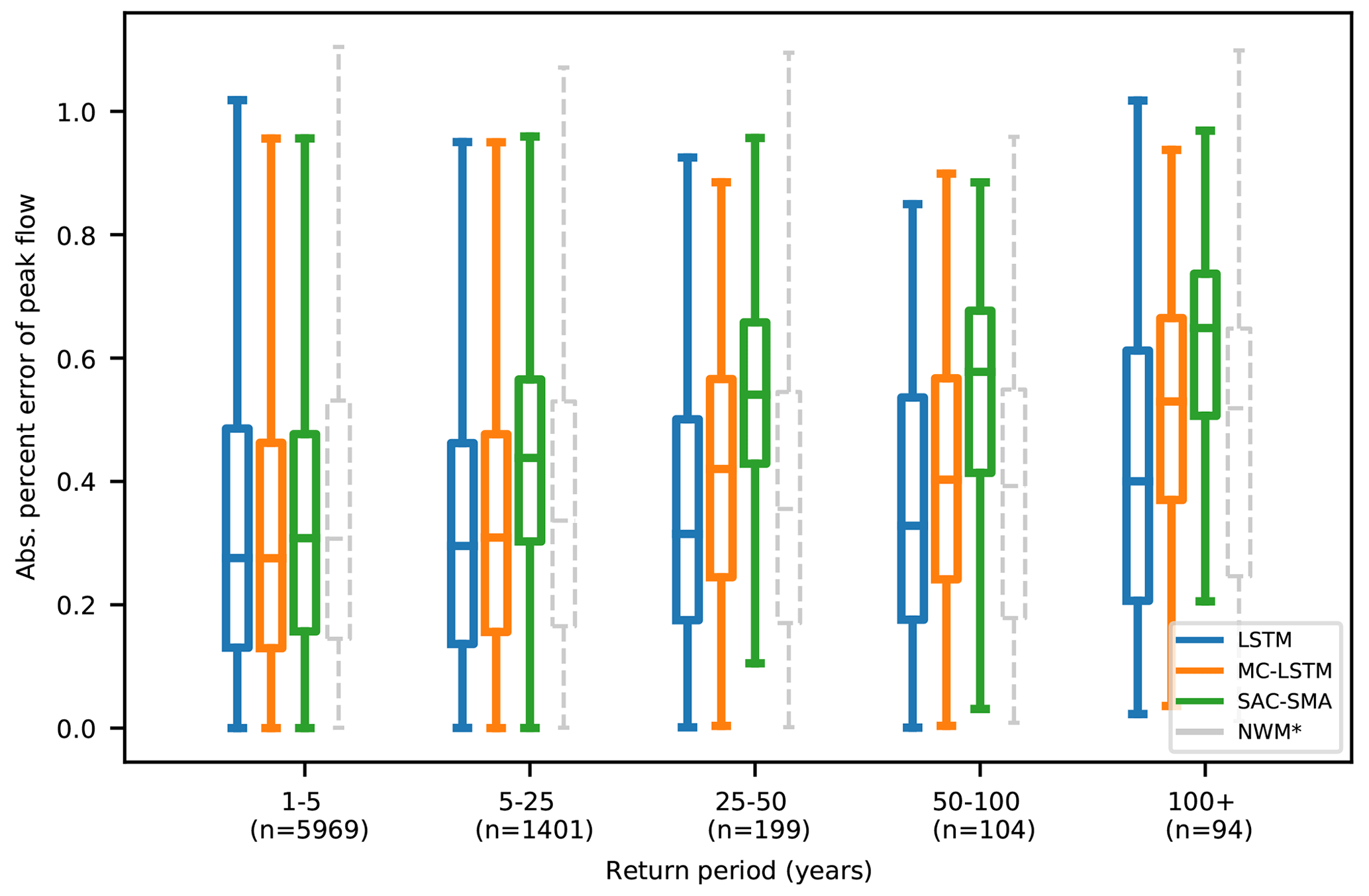
Figure 1 Average absolute percent bias of daily peak flow estimates from four models binned down by return period, showing results from models trained on a contiguous time period that contains a mix of different peak annual return periods. All statistics shown are calculated on test period data. The LSTM, MC-LSTM, and SAC-SMA models were all trained (calibrated) on the same data and time period. The NWM was calibrated on the same forcing data but on a different time period.

The second test period (1995–2014) allows us to benchmark against NWM-Rv2, which does not provide data prior to 1995. Most of these scores are broadly equivalent to the metrics for the same models reported for the test period from 1989 to 1999, with the exception of the FHV (high flow bias), FLV (low flow bias), and FMS (flow duration curve bias). These metrics depend heavily on the observed flow characteristics during a particular test period and, because they are less stable, are somewhat less useful in terms of drawing general conclusions. We report them here primarily for continuity with previous studies (Kratzert et al., 2019b, a, 2021; Frame et al., 2021; Nearing et al., 2020a; Klotz et al., 2021; Gauch et al., 2021), and because one of the objectives of this paper (Sect. 2.2) is to expand on the high-flow (FHV) analysis by benchmarking on annual peak flows.

The third test period (based on return periods) allows us to benchmark only on water years that contain streamflow events that are larger (per basin) than anything seen in the training data (≤ 5-year return periods in training and > 5-year return periods in testing). Model performance generally improves overall in this period according to the three correlation-based metrics (NSE, KGE, Pearson-r), but it degrades according to the variance-based metric (α-NSE). This is expected due to the nature of the metrics themselves – hydrology models generally exhibit a higher correlation with observations under wet conditions, simply due to higher variability. However, the data-driven models remained better than both benchmark models against all four of these metrics, and while the bias metric (β-NSE) was less consistent across test periods, the data-driven models had less overall bias than both benchmark models in the return period test period.

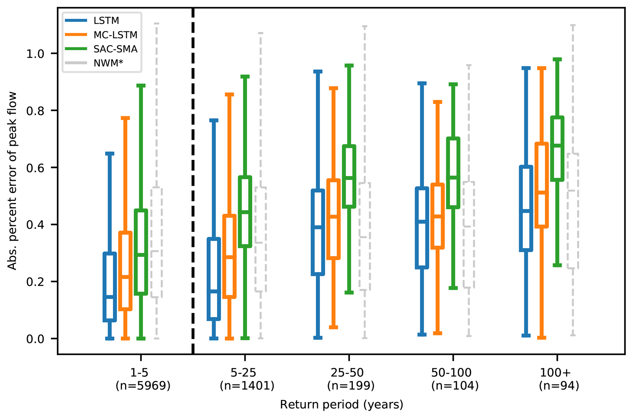
Figure 2 Average absolute percent bias of daily peak flow estimates from four models binned down by return period, showing results from models trained only on water years with return periods less than 5 years. The 1- to 5-year return period bin (left of the black dashed line) shows statistics calculated on training data, whereas bins with return periods of more that 5 years (to the right of the black dashed line) show statistics calculated on testing data. The LSTM, MC-LSTM, and SAC-SMA models were all trained (calibrated) on the same data and time period. The NWM was calibrated on the same forcing data but on a contiguous time period that does not exclude extreme events, as described in Sect. 2.3.2.

The results in Table 2 indicate broadly similar performance between the LSTM and MC-LSTM across most metrics in the two nominal (i.e., unbiased) test periods. However, there were small differences. The MC-LSTM generally performed slightly worse according to most metrics and test periods. The cross-comparison was mixed according to the timing-based metric (Peak-Timing). Notably, differences between the two ML-based models were small compared with the differences between these models and the conceptual (SAC-SMA) and process-based (NWM-Rv2) models, which both performed substantively worse across all metrics except FLV and FMS. The results also indicate that the MC-LSTM performs much worse according to the FLV metric, but we caution that the FLV metric is fragile, particularly when flows approach zero (due to dry or frozen conditions). The large discrepancy comes from several outlier basins that are regionally clustered, mostly around the southwest. The FLV equation includes a log value of the simulated and observed flows. This causes a very large instability in the calculation. Flow duration curves (and the flow duration curve of the minimum 30 % of flows) of the LSTM and the MC-LSTM are qualitatively similar, but they diverge on the low flow in terms of log values.

There were clear differences between the physics-constrained (MC-LSTM) and unconstrained (LSTM) data-driven models in the high-return-period metrics. While both data-driven models performed better than both benchmark models in these out-of-sample events, adding mass balance constraints resulted in reduced performance in the out-of-sample years.

The MC-LSTM includes a flux term that accounts for unobserved sources and sinks (e.g., evapotranspiration, sublimation, percolation). However, it is important to note that most or all hydrology models that are based on closure equations include a residual term in some form. Like all mass balance models, the MC-LSTM explicitly accounts for all water in and across the boundaries of the system. In the case of the MC-LSTM, this residual term is a single, aggregated flux that is parameterized with weights that are shared across all 498 basins. Even with this strong constraint, the MC-LSTM performs significantly better than the physically based benchmark models. This result indicates that classical hydrology model structures (conceptual flux equations) actually cause larger prediction errors than can be explained as being due to errors in the forcing and observation data.

3.2 Benchmarking peak flows

Figure 1 shows the average absolute percent bias of annual peak flows for water years with different return periods. The training/calibration period for these results is the contiguous test period (water years 1996–2014). All models had increasingly large average errors with increasingly large extreme events. The LSTM average error was lowest in all of the return period bins. SAC-SMA was the worst performing model in terms of average error. SAC-SMA was trained (calibrated) on the same data as the LSTM and MC-LSTM, and its performance decreased substantively with increasing return period whereas that of the LSTM did not.

Figure 2 shows the average absolute percent bias of annual peak flows for water years with different return periods, from models with a training/test split based on return periods, with all test data coming from water years 1996–2014. This means that Figs. 1 and 2 are only partially comparable – all statistics for each return period bin were calculated on the same observation data. All of the data shown in Fig. 1 come from the test period. However, as all water years with return periods of less than 5 years were used for training in the return-period-based training/test split, the 1- to 5-year return period category in Fig. 2 shows metrics calculated on training data. Thus, these two figures show only relative trends.

For the return period test (Fig. 2), the LSTM, MC-LSTM, and SAC-SMA were trained on data from all water years in 1980–2014 with return periods smaller than or equal to 5 years, and all of the models showed substantively better average performance in the low-return-period (high-probability) events than in the high-return-period (low-probability) events. SAC-SMA performance deteriorated faster than LSTM and MC-LSTM performance with increasingly extreme events. The unconstrained data-driven model (LSTM) performed better on average than all physics-informed and physically based models in predicting extreme events in all out-of-sample training cases except for the 25–50 and 50–100 cases, where NWM-Rv2 performed slightly better on average. However, remember that the NWM-Rv2 calibration data were not segregated by return period.

4 Conclusions and discussion

The hypothesis tested in this work was that predictions made by data-driven streamflow models are likely to become unreliable in extreme or out-of-sample events. This is an important hypothesis to test because it is a common concern among physical scientists and among users of model-based information products (e.g., Todini, 2007). However, prior work (e.g., Kratzert et al., 2019b; Gauch et al., 2021) has demonstrated that predictions made by data-based rainfall–runoff models are more reliable than other types of physically based models, even in extrapolation to ungauged basins (Kratzert et al., 2019a). Our results indicate that this hypothesis is incorrect: the data-driven models (both the pure ML model and the physics-informed ML model) were better than benchmark models at predicting peak flows under almost all conditions, including extreme events or when extreme events were not included in the training data set.

It was somewhat surprising to us that the physics-constrained LSTM did not perform as well as the pure LSTM at simulating peak flows and out-of-sample events. This surprised us for two reasons. First, we expected that adding closure would help in situations where the model sees rainfall events that are larger than anything it had seen during training. In this case, the LSTM could simply “forget” water, whereas the MC-LSTM would have to do something with the excess water – either store it in cell states or release it through one of the output fluxes. Second, Hoedt et al. (2021) reported that the MC-LSTM had a lower bias than the LSTM on 98th percentile streamflow events (this is our FHV metric). Our comparison between different training/test periods showed that FHV is a volatile metric, which might account for this discrepancy. The analysis by Hoedt et al. (2021) also did not consider whether a peak flow event was similar or dissimilar to training data, and we saw the greatest differences between the LSTM and MC-LSTM when predicting out-of-sample return period events.

This finding (differences between pure ML and physics-informed ML) is worth discussing. The project of adding physical constraints to ML is an active area of research across most fields of science and engineering (Karniadakis et al., 2021), including hydrology (e.g., Zhao et al., 2019; Jiang et al., 2020; Frame et al., 2021). It is important to understand that there is only one type of situation in which adding any type of constraint (physically based or otherwise) to a data-driven model can add value: if constraints help optimization. Helping optimization is meant here in a very general sense, which might include processes such as smoothing the loss surface, casting the optimization into a convex problem, or restricting the search space. Neural networks (and recurrent neural networks) can emulate large classes of functions (Hornik et al., 1989; Schäfer and Zimmermann, 2007); by adding constraints to this type of model, we can only restrict (not expand) the space of possible functions that the network can emulate. This form of regularization is valuable only if it helps locate a better (in some general sense) local minimum on the optimization response surface (Mitchell, 1980). Moreover, it is only in this sense that the constraints imposed by physical theory can add information relative to what is available purely from data.

Appendix A: LSTM

Long short-term memory networks (Hochreiter and Schmidhuber, 1997) represent time-evolving systems using a recurrent network structure with an explicit state space. Although LSTMs are not based on physical principles, Kratzert et al. (2018) argued that they are useful for rainfall–runoff modeling because they represent dynamic systems in a way that corresponds to physical intuition; specifically, LSTMs are Markovian in the (weak) sense that the future depends on the past only conditionally through the present state and future inputs. This type of temporal dynamics is implemented in an LSTM using an explicit input–state–output relationship that is conceptually similar to most hydrology models.

The LSTM architecture (Fig. A1) takes a sequence of input features $\mathit{x}=\left[\mathit{x}\right[\mathrm{1}],\mathrm{\dots },\mathit{x}[T\left]\right]$ of data over T time steps, where each element x[t] is a vector containing features at time step t. A vector of recurrent “cell states” c is updated based on the input features and current cell state values at time t. The cell states also determine LSTM outputs or hidden states, h[t] , which are passed through a “head layer” that combines the LSTM outputs (that are not associated with any physical units) into predictions $\widehat{\mathit{y}}\left[t\right]$ that attempt to match the target data (which may or may not be associated with physical units).

The LSTM structure (without the head layer) is as follows:

$$\begin{array}{}\text{(A1)}& {\displaystyle }\mathit{i}\left[t\right]=\mathit{\sigma }\left({\mathbf{W}}_i\mathit{x}\right[t]+{\mathbf{U}}_i\mathit{h}[t-\mathrm{1}]+{\mathit{b}}_{\mathit{i}})\text{(A2)}& {\displaystyle }\mathit{f}\left[t\right]=\mathit{\sigma }\left({\mathbf{W}}_f\mathit{x}\right[t]+{\mathbf{U}}_f\mathit{h}[t-\mathrm{1}]+{\mathit{b}}_{\mathit{f}})\text{(A3)}& {\displaystyle }\mathit{g}\left[t\right]=\tanh \left({\mathbf{W}}_g\mathit{x}\right[t]+{\mathbf{U}}_g\mathit{h}[t-\mathrm{1}]+{\mathit{b}}_{\mathit{g}})\text{(A4)}& {\displaystyle }\mathit{o}\left[t\right]=\mathit{\sigma }\left({\mathbf{W}}_o\mathit{x}\right[t]+{\mathbf{U}}_o\mathit{h}[t-\mathrm{1}]+{\mathit{b}}_{\mathit{o}})\text{(A5)}& {\displaystyle }\mathit{c}\left[t\right]=\mathit{f}\left[t\right]\odot \mathit{c}[t-\mathrm{1}]+\mathit{i}\left[t\right]\odot \mathit{g}\left[t\right]\text{(A6)}& {\displaystyle }\mathit{h}\left[t\right]=\mathit{o}\left[t\right]\odot \tanh \left(\mathit{c}\right[t\left]\right)\end{array}$$

The symbols i[t], f[t], and o[t] refer to the “input gate”, “forget gate”, and “output gate” of the LSTM, respectively; g[t] is the “cell input” and x[t] is the “network input” at time step t; h[t−1] is the LSTM output, which is also called the “recurrent input” because it is used as inputs to all gates in the next time step; and c[t−1] is the cell state from the previous time step.

Cell states represent the memory of the system through time, and they are initialized as a vector of zeros. σ(⋅) are sigmoid activation functions, which return values in [0,1]. These sigmoid activation functions in the forget gate, input gate, and output gate are used in a way that is conceptually similar to on–off switches – multiplying anything by values in [0,1] is a form of attenuation. The forget gate controls the memory timescales of each of the cell states, and the input and output gates control flows of information from the input features to the cell states and from the cell states to the outputs (recurrent inputs), respectively. W, U, and b are calibrated parameters, where subscripts indicate which gate the particular parameter matrix/vector is associated with. tanh(⋅) is the hyperbolic tangent activation function, which serves to add nonlinearity to the model in the cell input and recurrent input, and ⊙ indicates element-wise multiplication. For a hydrological interpretation of the LSTM, see Kratzert et al. (2018).

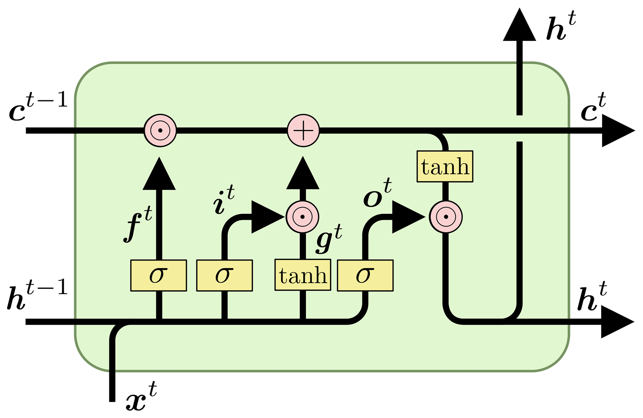
Figure A1 A single time step of a standard LSTM, with time steps marked as superscripts for clarity. x^t, c^t, and h^t are the input features, cell states, and recurrent inputs at time t, respectively. f^t, i^t, and o^t are the respective forget gates, input gates, and output gates, and g^t denotes the cell input. Boxes labeled σ and tanh represent respective single sigmoid and hyperbolic tangent activation layers with the same number of nodes as cell states. The addition sign represents element-wise addition, and ⊙ represents element-wise multiplication.

Appendix B: MC-LSTM

The LSTM has an explicit input–state–output structure that is recurrent in time and is conceptually similar to how physical scientists often model dynamical systems. However, the LSTM does not obey physical principles, and the internal cell states have no physical units. We can leverage this input–state–output structure to enforce mass conservation, in a manner that is similar to discrete-time explicit integration of a dynamical systems model, as follows:

$$\begin{array}{}\text{(B1)}& \mathrm{new}\mathrm{states}=\mathrm{old}\mathrm{states}+\mathrm{inputs}-\mathrm{outputs}.\end{array}$$

Using the notation from Appendix A, this is

$$\begin{array}{}\text{(B2)}& {\mathit{c}}^{\mathbf{*}}\left[t\right]={\mathit{c}}^{\mathbf{*}}[t-\mathrm{1}]+{\mathit{x}}^{\mathbf{*}}\left[t\right]-{\mathit{h}}^{\mathbf{*}}\left[t\right],\end{array}$$

where c^*[t], x^*[t], and h^*[t] are components of the cell states, input features, and model outputs (recurrent inputs) that contribute to a particular conservation law.

As presented by Hoedt et al. (2021), we can enforce conservation in the LSTM by doing two things. First, we use special activation functions in some of the gates to guarantee that mass is conserved from the inputs and previous cell states. Second, we subtract the outgoing mass from the cell states. The important property of the special activation functions is that the sum of all elements sum to 1. This allows the outputs of each activation node to be scaled by a quantity that we want to conserve, so that each scaled activation value represents a fraction of that conserved quantity. In practice, we can use any standard activation function (e.g., sigmoid or rectified linear unit – ReLU) as long as we normalize the activation. With positive activation functions, we can, for example, normalize by the L1 norm (see Eqs. B3 and B4). Another option would be to use the softmax activation function, which sums to 1 by definition.

$$\begin{array}{}\text{(B3)}& {\displaystyle }\widehat{\mathit{\sigma }}\left(s_k\right)& {\displaystyle }={\displaystyle \frac{\mathit{\sigma }\left(s_k\right)}{{\sum }_k\mathit{\sigma }\left(s_k\right)}}\text{(B4)}& {\displaystyle }\widehat{\mathrm{ReLU}}\left(s_k\right)& {\displaystyle }={\displaystyle \frac{\max (s_k,\mathrm{0})}{{\sum }_k\max (s_k,\mathrm{0})}}\end{array}$$

The constrained model architecture is illustrated in Fig. B1. An important difference with the standard architecture is that the inputs are separated into “mass inputs” x and “auxiliary inputs” a. In our case, the mass input is precipitation and the auxiliary inputs are everything else (e.g., temperature, radiation, catchment attributes). The input gate (sigmoids) and cell input (hyperbolic tangents) in the standard LSTM are (collectively) replaced by one of these normalization layers, while the output gate is a standard sigmoid gate, similar to the standard LSTM. The forget gate is also replaced by a normalization layer, with the important difference that the output of this layer is a square matrix with dimension equal to the size of the cell state. This matrix is used to “reshuffle” the mass between the cell states at each time step. This “reshuffling matrix” is column-wise normalized so that the dot product with the cell state vector at time t results in a new cell state vector having the same absolute norm (so that no mass is lost or gained).

We call this general architecture a mass-conserving LSTM (MC-LSTM), even though it works for any type of conservation law (e.g., mass, energy, momentum, counts). The architecture is illustrated in Fig. B1 and is described formally as follows:

$$\begin{array}{}\text{(B5)}& {\displaystyle }\widehat{\mathit{c}}[t-\mathrm{1}]={\displaystyle \frac{\mathit{c}[t-\mathrm{1}]}{\left|\right|\mathit{c}[t-\mathrm{1}]|{|}_{\mathrm{1}}}}\text{(B6)}& {\displaystyle }\mathit{i}\left[t\right]=\widehat{\mathit{\sigma }}\left({\mathbf{W}}_i\mathit{x}\right[t]+{\mathbf{U}}_i\widehat{\mathit{c}}[t-\mathrm{1}]+{\mathbf{V}}_i\mathit{a}[t]+{\mathit{b}}_i)\text{(B7)}& {\displaystyle }\mathit{o}\left[t\right]=\mathit{\sigma }\left({\mathbf{W}}_o\mathit{x}\right[t]+{\mathbf{U}}_o\widehat{\mathit{c}}[t-\mathrm{1}]+{\mathbf{V}}_o\mathit{a}[t]+{\mathit{b}}_{\mathit{o}})\text{(B8)}& {\displaystyle }\mathbf{R}\left[t\right]=\widehat{\mathrm{ReLU}}\left({\mathbf{W}}_{\mathbf{R}}\mathit{x}\right[t]+{\mathbf{U}}_{\mathbf{R}}\widehat{\mathit{c}}[t-\mathrm{1}]+{\mathbf{V}}_{\mathbf{R}}\mathit{a}[t]+{\mathit{b}}_{\mathbf{R}})\text{(B9)}& {\displaystyle }\mathit{m}\left[t\right]=\mathbf{R}\left[t\right]\mathit{c}[t-\mathrm{1}]+\mathit{i}\left[t\right]\mathit{x}\left[t\right]\text{(B10)}& {\displaystyle }\mathit{c}\left[t\right]=(\mathrm{1}-\mathit{o}[t\left]\right)\odot \mathit{m}\left[t\right]\text{(B11)}& {\displaystyle }\mathit{h}\left[t\right]=\mathit{o}\left[t\right]\odot \mathit{m}\left[t\right]\end{array}$$

Learned parameters are W, U, V, and b for all of the gates. The normalized activation functions are, in this case, $\widehat{\mathit{\sigma }}$ (see Eq. B3) for the input gate and $\widehat{\mathrm{ReLU}}$ (see Eq. B4) for the redistribution matrix R, as in the hydrology example of Hoedt et al. (2021). The products of i[t]x[t] and o[t]⊙m[t] are input and output fluxes, respectively.

Because this model structure is fundamentally conservative, all cell states and information transfers within the model are associated with physical units. Our objective in this study was to maintain the overall water balance in a catchment – our conserved input feature, x, is precipitation (in units of mm d⁻¹) and our training targets are catchment discharge (also in units of mm d⁻¹). Thus, all input fluxes, output fluxes, and cell states in the MC-LSTM have units of millimeters per day (mm d⁻¹).

In reality, precipitation and streamflow are not the only fluxes of water into or out of a catchment. Because we did not provide the model with (for example) observations of evapotranspiration, aquifer recharge, or baseflow, we accounted for unobserved sinks in the modeled systems by allowing the model to use one cell state as a “trash cell”. The output of this cell is ignored when we derive the final model prediction as the sum of the outgoing mass ∑h.

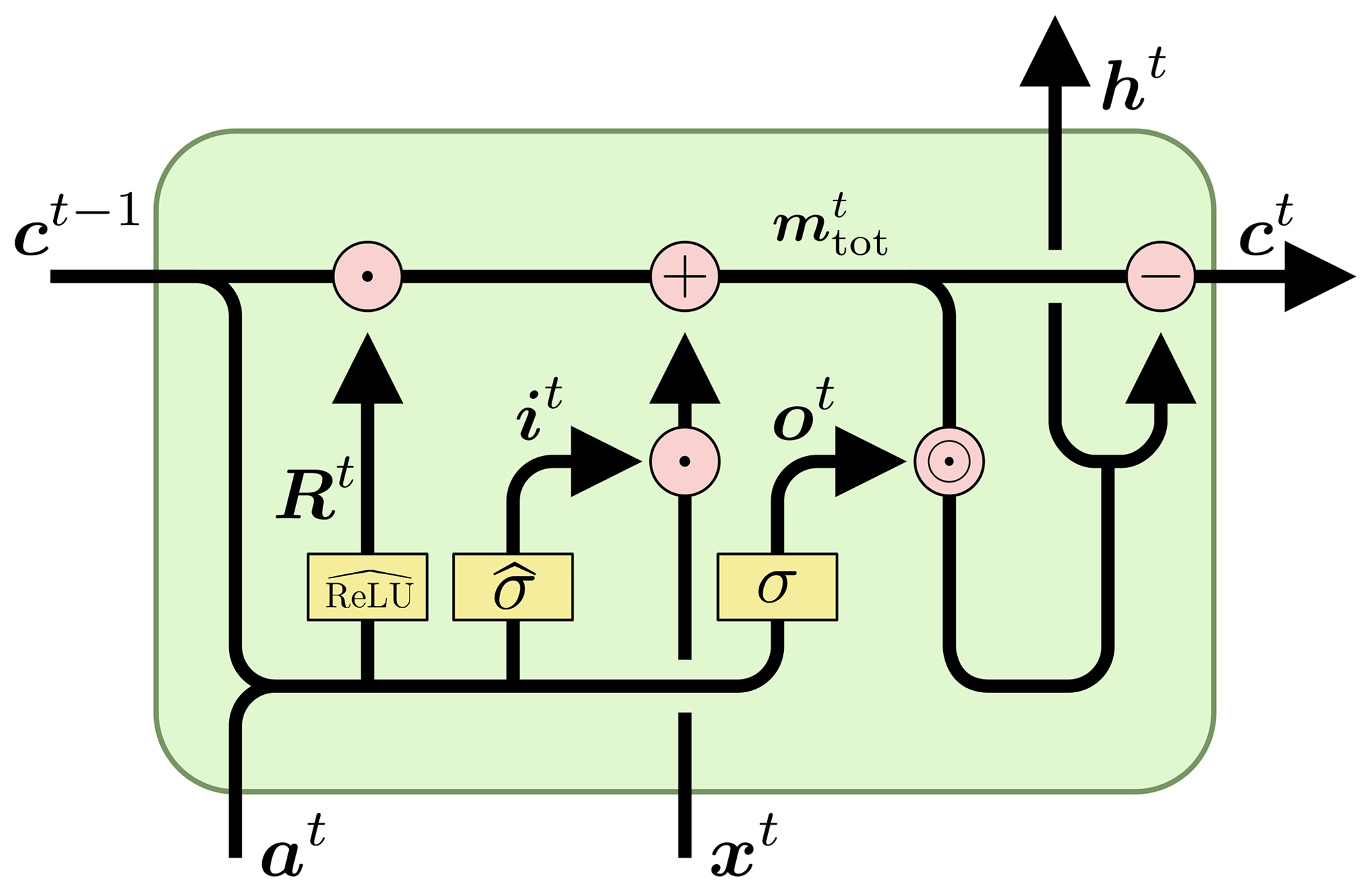
Figure B1 A single time step of a mass-conserving LSTM, with time steps marked as superscripts for clarity. As in Fig. A1, c^t, a^t, x^t, i^t, o^t, and R^t are the cell states, conserved inputs, input features, input fluxes, output fluxes, and reshuffling matrix at time t, respectively. σ represents a standard sigmoid activation layer, and $\widehat{\mathit{\sigma }}$ and $\widehat{\mathrm{ReLU}}$ represent normalized sigmoid activation layers and normalized ReLU activation layers, respectively. Addition and subtraction signs represent element-wise addition and subtraction, respectively; ⊙ represents element-wise multiplication; and the ⋅ sign represents the dot product.

Appendix C: Benchmarking annual return period metrics

Figure C1 shows nine performance metrics calculated on model test results split into bins according to the return period of the peak annual flow event. The LSTM, MC-LSTM, and SAC-SMA were calibrated/trained on water years 1981–1995. The results shown in this figure are for water years 1996–2014. The LSTM and MC-LSTM perform better than the benchmark models according to most metrics and during most return period bins. There are a few instances where NWM-Rv2 performs better than the LSTM and/or the MC-LSTM. The NWM-Rv2 calibration, which was carried out by NOAA personnel on about 1400 basins with NLDAS forcing data on water years 2009–2013, does not correspond to the training/calibration period of SAC-SMA, LSTM, or MC-LSTM.

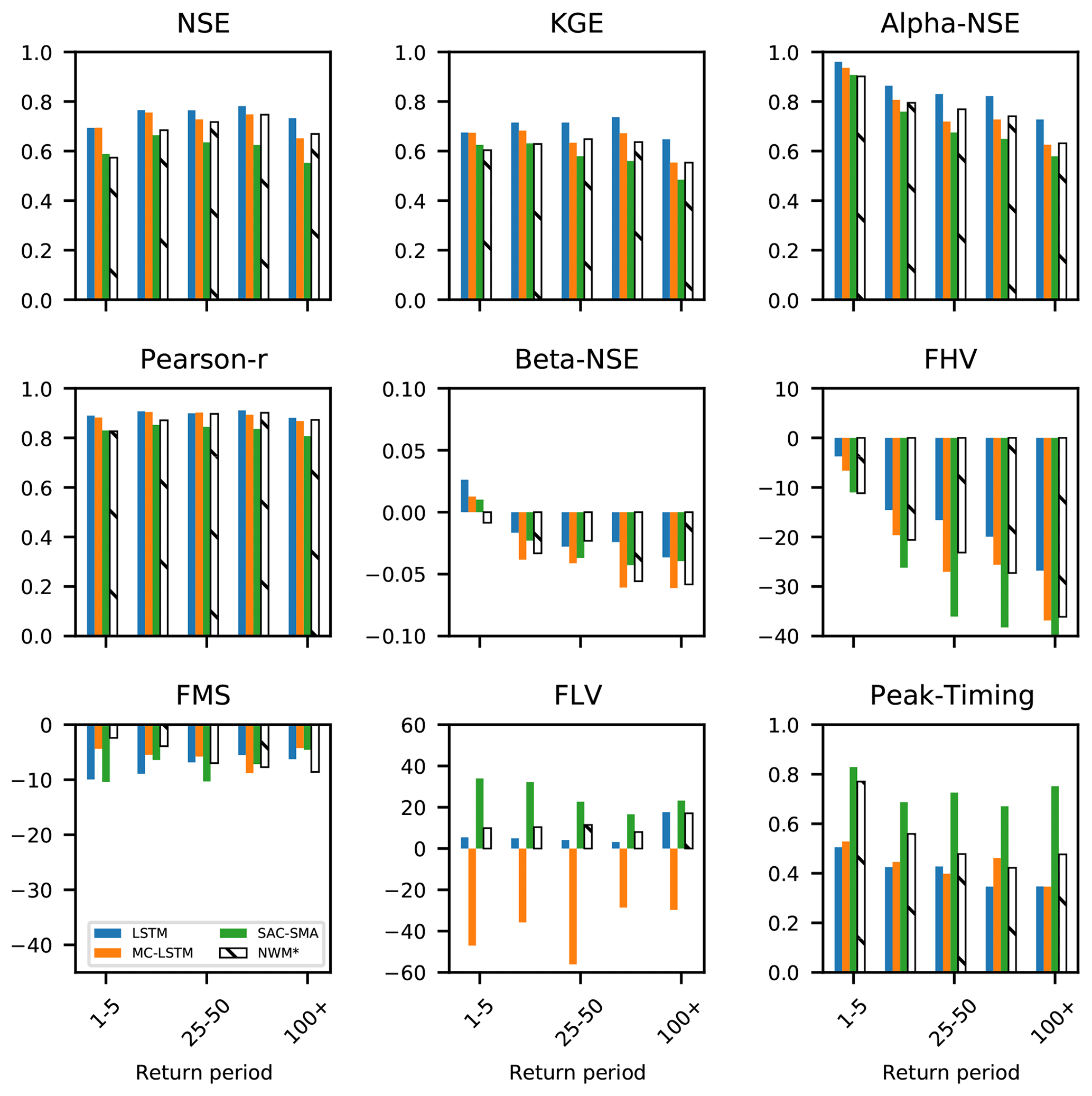
Figure C1 Metrics for training only on a standard time split; the training period was water years 1981–1995, and the test period (shown here) was water years 1996-2014. The total number of samples in each bin is as follows: n=5969 for 1–5, n=1260 for 5–25, n=185 for 25–50, n=91 for 50–100, and n=84 for 100 +.

Figure C2 shows the nine performance metrics calculated on model test results split into bins according to the return period of the peak annual flow event. The LSTM, MC-LSTM, and SAC-SMA were calibrated/trained on water years with a peak annual flow event that had a return period of less that 5 years (i.e., bin 1–5 indicated by the dashed line). The results shown in this figure are for water years 1996–2014. The LSTM and MC-LSTM perform better than the SAC-SMA model according to every metric and during all bins. There are a few instances where NWM-Rv2 performs better than the LSTM and/or the MC-LSTM. The NWM-Rv2 calibration does not correspond to the training/calibration period of SAC-SMA, LSTM, or MC-LSTM.

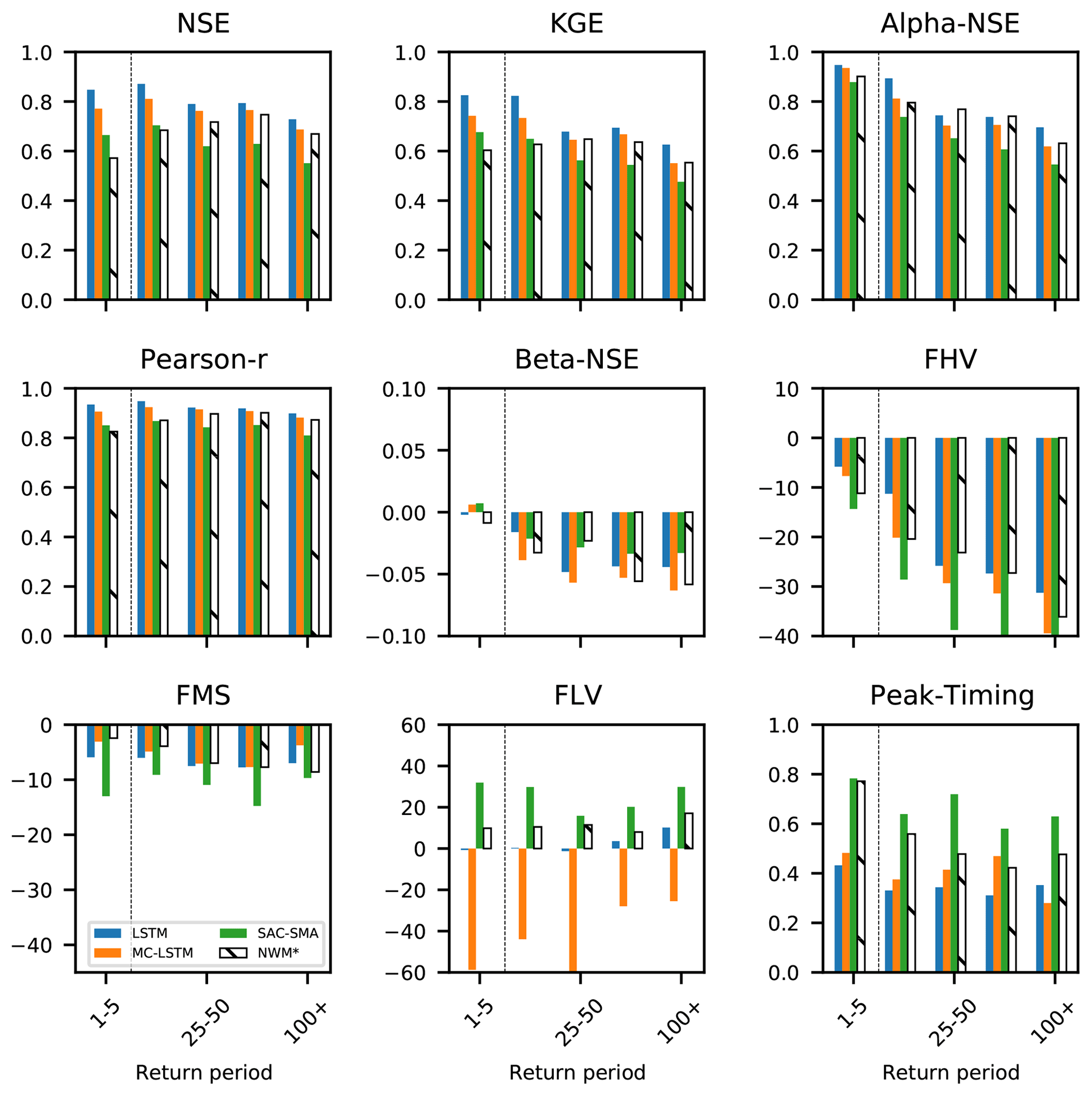
Figure C2 Metrics for the models trained only on high-probability years. The bins of return periods greater than 5 are out of sample for the LSTM, MS-LSTM, and SAC-SMA. The total number of samples in each bin is as follows: n=5969 for 1–5, n=1260 for 5–25, n=185 for 25–50, n=91 for 50–100, and n=84 for 100 +.